Relating the Entanglement and Optical Nonclassicality
of Multimode States of a Bosonic Quantum Field

Abstract

The quantum nature of the state of a bosonic quantum field may manifest itself in its entanglement, coherence, or optical nonclassicality. Each of these distinct properties is known to be a resource for quantum computing or metrology, and can be evaluated via a variety of measures, witnesses, or monotones. Here, we provide quantitative and computable bounds relating, in particular, some entanglement measures with optical nonclassicality measures. Overall, these bounds capture the fact that strongly entangled states must necessarily be strongly optically nonclassical. As an application, we infer strong bounds on the entanglement that can be produced with an optically nonclassical state impinging on a beam splitter. Then, focusing on Gaussian states, we analyze the link between the logarithmic negativity and a specific nonclassicality measure called “quadrature coherence scale”.

I Introduction

There are several ways to question the specifically quantum mechanical character of the state of a physical system. First, one may ask how strongly coherent it is. The existence of coherent superpositions of quantum states is at the origin of interference phenomena in matter waves and, as such, is a typically quantum feature for which several measures and witnesses have been proposed (for a recent review, see Streltsov et al. (2017)). Second, when the system under investigation is bi-partite or multi-partite, the entanglement of its components is another intrinsically quantum feature. There exists an extensive literature exploring a wide variety of measures to quantify the amount of entanglement contained in a given state Horodecki et al. (1996); Peres (1996); Bennett et al. (1996); Duan et al. (2000); Simon (2000); Werner and Wolf (2001); Vidal and Werner (2002); Serafini et al. (2005); Shchukin and Vogel (2005); Rudolph (2005); Horodecki et al. (2009); Walborn et al. (2009); Zhang et al. (2013). Finally, for modes of a bosonic quantum field, a third notion of nonclassicality arises, which is often refered to as optical nonclassicality. Following Glauber, the coherent states of an optical field (as well as their mixtures) are viewed as “classical” as they admit a positive Glauber-Sudarshan P-function Titulaer and Glauber (1965). From there, a variety of measures of optical nonclassicality have been developed over the years, measuring the departure from such optical classical states Titulaer and Glauber (1965); Hillery (1985); Bach and Lüxmann-Ellinghaus (1986); Hillery (1987, 1989); Lee (1991); Agarwal and Tara (1992); Lee (1995); Lütkenhaus and Barnett (1995); Dodonov et al. (2000); Marian et al. (2002); Richter and Vogel (2002); Kenfack and Zyczkowski (2004); Asbóth et al. (2005); Semenov et al. (2006); Zavatta et al. (2007); Vogel and Sperling (2014); Ryl et al. (2015); Sperling and Vogel (2015); Killoran et al. (2016); Alexanian (2017); Nair (2017); Ryl et al. (2017); Yadin et al. (2018); Kwon et al. (2019); De Bièvre et al. (2019); Luo and Zhang (2019).

Each of these three distinct, typically quantum properties of the state of an optical field have been argued to serve as a resource in quantum information or metrology Yadin et al. (2018); Kwon et al. (2019); Friis et al. (2015); Sahota and Quesada (2015); Ge et al. (2018). The question then naturally arises what the quantitative relations are between these properties. In Streltsov et al. (2015), for example, bounds are given on how much entanglement can be produced from states with a given amount of coherence using incoherent operations: this links coherence with entanglement. In Hertz and De Bièvre (2020), the coherence and optical nonclassicality of a state are shown to be related to each other: a large value of far off-diagonal density matrix elements $\rho(x,x^{\prime})$ or $\rho(p,p^{\prime})$, called “coherences”, is a witness of the optical nonclassicality of the state. Our purpose here is to establish a relation between optical nonclassicality and bi-partite entanglement for multi-mode bosonic fields.

One expects on intuitive grounds that a strongly entangled state should be strongly optically nonclassical since all optical classical states are separable. Conversely, a state that is only weakly optically nonclassical cannot possibly be highly entangled. To make these statements precise and quantitative, we need both a measure of entanglement and one of optical nonclassicality. As a natural measure to evaluate bi-partite entanglement, we use the entanglement of formation ($\mathcal{E}_{F}$) Bennett et al. (1996). Regarding optical nonclassicality, we use a recently introduced monotone Yadin et al. (2018); Kwon et al. (2019), which we refer to as the monotone of total noise (${{\mathcal{M}}_{\textrm{TN}}}$). It is obtained by extending to mixed states [through a convex roof construction, see (1)] the so-called total noise $\Delta x^{2}+\Delta p^{2}$ defined on pure states, for which it is a well established measure of optical nonclassicality Yadin et al. (2018); Kwon et al. (2019); De Bièvre et al. (2019); Luo and Zhang (2019). Our first main result (Theorems 1 & 1’) consists in an upper bound on $\mathcal{E}_{F}(\rho)$ as a function of ${{\mathcal{M}}_{\textrm{TN}}}(\rho)$ for an arbitrary state $\rho$ of a bi-partite system of $n=n_{A}+n_{B}$ modes. In particular, when $n_{A}=n_{B}=n/2$, this bound implies that states containing $m$ ebits of entanglement must have an optical nonclassicality – measured via ${{\mathcal{M}}_{\textrm{TN}}}$ – that grows exponentially with $m$. As an application, we show that the maximum entanglement that can be produced when a separable pure state impinges on a balanced beam splitter is bounded by the logarithm of the optical nonclassicality of this in-state, measured by ${{\mathcal{M}}_{\textrm{TN}}}$. In other words, while it is well known that beam splitters can produce entanglement Kim et al. (2002); Xiang-bin (2002); Asbóth et al. (2005), the amount of entanglement so produced is shown to be severely constrained by the degree of optical nonclassicality of the in-state. More precisely, the amount of nonclassicality needed in the in-state grows exponentially with the number of e-bits of entanglement required at the output. Since it was shown in Hertz and De Bièvre (2020) that strongly optically nonclassical states are extremely sensitive to environmental decoherence which destroys their nonclassicality on a very short timescale, these results imply it is very difficult to produce strongly entangled states with a beam splitter in the above manner.

The bounds in Theorems 1 & 1’ can readily be computed for pure states since $\mathcal{E}_{F}$ then coincides with the von Neumann entropy of the reduced state and ${{\mathcal{M}}_{\textrm{TN}}}$ coincides with the total noise. For mixed states, however, the bounds relate two quantities that are generally hard to evaluate. Our second main result (Theorem 2) addresses this issue by considering the special case of (mixed) Gaussian states. It establishes bounds between explicitly computable measures of entanglement (the logarithmic negativity – $\mathcal{E}_{\mathcal{N}}$) and optical nonclassicality (the quadrature coherence scale – ${\mathcal{C}}$) for Gaussian states. We also derive an explicit simple formula for the quadrature coherence scale of Gaussian states in terms of their covariance matrix [see Eq. (16)]. We show that it actually coincides with its Total Quantum Fisher Information ($\mathcal{F}_{\text{tot}}$), a quantity of importance in metrology which has been shown to provide a nonclassicality monotone Yadin et al. (2018); Kwon et al. (2019), albeit not a faithful one.

II Bounding $\mathcal{E}_{F}$ by optical nonclassicality.

We consider an $n$-mode optical field with annihilation mode operators $a_{i}=(X_{i}+iP_{i})/\sqrt{2}$ and corresponding quadratures $X_{i}$, $P_{i}$. We set ${\mathbf{R}}=(X_{1},P_{1},\dots,X_{n},P_{n})$. The total noise of a pure state $|\psi\rangle$ is defined as ${\mathcal{N}}_{\textrm{tot}}(\psi)=\sum_{j}\Delta R_{j}^{2}$ where $\Delta R_{j}^{2}$ denotes the variance of $R_{j}$ Schumaker (1986). For a general state $\rho$, the convex roof ${{\mathcal{M}}_{\textrm{TN}}}$ of ${\mathcal{N}}_{\textrm{tot}}$ is

$${{\mathcal{M}}_{\textrm{TN}}}(\rho)=\frac{1}{n}\inf_{\{p_{i},\psi_{i}\}}\sum_{i}p_{i}\,{\mathcal{N}}_{\textrm{tot}}(\psi_{i})\geq 1,$$ (1)

where the infimum is over all ensembles $\{p_{i},\psi_{i}\}$ for which $\rho=\sum_{i}p_{i}|\psi_{i}\rangle\langle\psi_{i}|$, $\sum_{i}p_{i}=1$. It is shown in Yadin et al. (2018); Kwon et al. (2019) that ${{\mathcal{M}}_{\textrm{TN}}}$ belongs to a family of optical nonclassicality monotones and is, as such, a faithful witness of optical nonclassicality: ${{\mathcal{M}}_{\textrm{TN}}}(\rho)>1$ iff $\rho$ is nonclassical.

Now consider a bi-partition of the $n$ modes in two sets of $n_{A}$ and $n_{B}$ modes, with $n=n_{A}+n_{B}$. We write $\rho_{A}$ (respectively $\rho_{B}$) for the reduction of the state $\rho$ to the $n_{A}$ ($n_{B}$) modes. If $\rho=|\psi\rangle\langle\psi|$, its entanglement of formation is defined as $\mathcal{E}_{F}(\psi)=-\operatorname{Tr}\rho_{A}\ln\rho_{A}=-\operatorname{Tr}\rho_{B}\ln\rho_{B}$. Then, for a general $\rho$, taking the infimum as above Bennett et al. (1996),

$$\mathcal{\mathcal{E}_{F}}(\rho)=\inf_{\{p_{i},\psi_{i}\}}\sum_{i}p_{i}\,\mathcal{E}_{F}(\psi_{i}).$$

We first consider the symmetric case $n_{A}=n_{B}=n/2$:

Theorem 1

Let $\rho$ be a bipartite state with $n_{A}=n_{B}=n/2$, then

$$\mathcal{E}_{F}(\rho)\leq\frac{n}{2}\,g\left(\frac{1}{2}\left({{\mathcal{M}}_{\textrm{TN}}}(\rho)-1\right)\right),$$ (2)

where $g(x)=(x+1)\ln(x+1)-x\ln x$.

Proof.

We first consider pure states $\rho=|\psi\rangle\langle\psi|$. Since both sides of (2) are invariant under phase space translations, we may assume that $\langle\psi|R_{j}|\psi\rangle=0$, $\forall j$. In that case, ${{\mathcal{M}}_{\textrm{TN}}}(\psi)=(2\langle\psi|\hat{N}|\psi\rangle+n)/n=2N/n+1$, where $N=\langle\psi|\hat{N}|\psi\rangle$ is the expectation value of the total photon number operator $\hat{N}=\sum_{j}a^{\dagger}_{j}a_{j}$ in the centered state $|\psi\rangle$. Similarly, defining $\hat{N}_{A}=~{}\sum_{j=1}^{n_{A}}a^{\dagger}_{j}a_{j}$ and $\hat{N}_{B}=\sum_{j=n_{A}+1}^{n}a^{\dagger}_{j}a_{j}$, one has $N_{A}=\operatorname{Tr}\hat{N}_{A}\rho_{A}$, $N_{B}=\operatorname{Tr}\hat{N}_{B}\rho_{B}$, and $N=N_{A}+N_{B}$. Then

$$\mathcal{E}_{F}(\psi) = -\operatorname{Tr}\rho_{A}\ln\rho_{A}=-\operatorname{Tr}\rho_{B}\ln\rho_{B}$$

$$\leq \min\left\{n_{A}\,g\left(\frac{N_{A}}{n_{A}}\right),n_{B}\,g\left(\frac{N_{B}}{n_{B}}\right)\right\},$$

where $n_{A}\,g(N_{A}/n_{A})$ is the von Neumann entropy of the product of $n_{A}$ single-mode thermal states with mean photon number $N_{A}/n_{A}$ per mode, which maximizes the von Neumann entropy at fixed mean photon number $N_{A}$ Wehrl (1978). Maximizing over all states $|\psi\rangle$ with a fixed mean photon number $N$ then yields

$$\mathcal{E}_{F}(\psi)\leq\max_{0\leq N_{A}\leq N}\min\left\{n_{A}\,g\left(\frac{N_{A}}{n_{A}}\right),n_{B}\,g\left(\frac{N-N_{A}}{n_{B}}\right)\right\}.$$

Since $g$ is an increasing function, the maximum is, for each $N$, reached at a unique value $N_{A}^{*}$ that depends on $N$ and is the solution of

$$n_{A}\,g\left(\frac{N_{A}^{*}}{n_{A}}\right)=n_{B}\,g\left(\frac{N-N_{A}^{*}}{n_{B}}\right).$$ (3)

Hence

$$\mathcal{E}_{F}(\psi)\leq n_{A}\,g(N_{A}^{*}/n_{A}):=F(N).$$ (4)

When $n_{A}=n_{B}$, then $N_{A}^{*}=N_{B}^{*}=N/2$, so that

$$\mathcal{E}_{F}(\psi)\leq\frac{n}{2}\,g\left(\frac{N}{n}\right)=\frac{n}{2}\,g\left(\frac{1}{2}({{\mathcal{M}}_{\textrm{TN}}}(\psi)-1)\right).$$ (5)

This implies Eq. (2) for any pure state $\rho=|\psi\rangle\langle\psi|$. Now let $\rho$ be an arbitrary state and consider any set of normalized $|\psi_{i}\rangle$ and $0\leq p_{i}\leq 1$ such that $\sum_{i}p_{i}|\psi_{i}\rangle\langle\psi_{i}|=\rho$. Then Eq. (5) and the concavity of $g$ imply that

$$\sum_{i}p_{i}\,\mathcal{E}_{F}({\psi_{i}}) \leq \frac{n}{2}\sum_{i}p_{i}\,g\left(\frac{1}{2}({{\mathcal{M}}_{\textrm{TN}}}(\psi_{i})-1)\right)$$

$$\leq \frac{n}{2}\,g\left(\frac{1}{2}\left(\sum_{i}p_{i}\,{{\mathcal{M}}_{\textrm{TN}}}(\psi_{i})-1\right)\right).$$

Since $g(x)$ is monotonically increasing, taking the infimum over $\{p_{i},\psi_{i}\}$ on both sides implies Eq. (2). ∎

One readily sees that, among all states $|\psi\rangle$ with a given $N$, the upper bound $\mathcal{E}_{F}(\psi)=\frac{n}{2}\,g\left(\frac{N}{n}\right)$ is reached for an $n/2$-fold tensor product of two-mode squeezed vacuum states with $N/n$ photons per mode, which is a Gaussian pure state. This is not the unique optimal pure state. We identify all such states in Appendix A and show they are not all Gaussian.

Since $g(x)$ is an increasing function, the bound (2) straightforwardly implies that states with a large entanglement of formations are necessarily strongly nonclassical:

Corollary 1

$$\mathcal{E}_{F}(\rho)\geq\frac{3}{2}\frac{n}{2}\ \ \Rightarrow\ \ {{\mathcal{M}}_{\textrm{TN}}}(\rho)\geq 1+2\,{\mathrm{e}}^{\frac{2}{n}\mathcal{E}_{F}(\rho)-2}.$$ (6)

Proof.

Suppose $\mathcal{E}_{F}(\rho)\geq\frac{3}{2}\frac{n}{2}$. Using Eq. (2), it implies that $g\left(\frac{1}{2}\left({{\mathcal{M}}_{\textrm{TN}}}(\rho)-1\right)\right)\geq\frac{3}{2}$. Noting that $g(x)\leq x+\frac{1}{2}$ for all $x$, one can conclude that $\frac{1}{2}({{\mathcal{M}}_{\textrm{TN}}}(\rho)-1)\geq 1$. Now, one also has $g(x)\leq\ln x+1+\frac{1}{x}$ for all $x>0$, and hence $g(x)\leq\ln x+2$ for all $x\geq 1$. Hence $g\left(\frac{1}{2}\left({{\mathcal{M}}_{\textrm{TN}}}(\rho)-1\right)\right)\leq\ln\left(\frac{1}{2}({{\mathcal{M}}_{\textrm{TN}}}(\rho)-1)\right)+2$. Using again Eq. (2) implies that $\mathcal{E}_{F}(\rho)\leq\frac{n}{2}\left(\ln\left(\frac{1}{2}({{\mathcal{M}}_{\textrm{TN}}}(\rho)-1)\right)+2\right),$ from which one concludes ${{\mathcal{M}}_{\textrm{TN}}}(\rho)\geq 1+2{\mathrm{e}}^{\frac{2}{n}\mathcal{E}_{F}(\rho)-2}$, which is Eq. (6). ∎

In other words, if we view both entanglement and optical nonclassicality as resources, this inequality shows that the amount of optical nonclassicality of a state $\rho$, as measured by ${{\mathcal{M}}_{\textrm{TN}}}(\rho)$, grows exponentially fast with its entanglement of formation, measured in number of ebits. Conversely, the bound (2) shows that states with a low optical nonclassicality are necessarily weakly entangled.

When $n_{A}\leq n_{B}$, Theorem 1 can be generalized as follows

Theorem 1’

Let $\rho$ be a bipartite state with $n_{A}\leq n_{B}$, then

$$\mathcal{E}_{F}(\rho)\leq n_{A}g\left(\frac{1}{n_{A}}N_{A}^{*}\left(\frac{n}{2}({{\mathcal{M}}_{\textrm{TN}}}(\rho)-1)\right)\right),$$ (7)

where $N_{A}^{*}(N)$ is the unique solution of Eq. (3).

Proof.

We first need to show that the function

$$F(N):=n_{A}\,g\left(\frac{N_{A}^{*}}{n_{A}}\right)$$

is concave, where $N_{A}^{*}$ is a function of $N$, implicitly defined as the solution of (3), $n_{A}\,g\left(\frac{N_{A}^{*}}{n_{A}}\right)=n_{B}\,g\left(\frac{N_{B}^{*}}{n_{B}}\right),$ where we defined $N_{B}^{*}=N-N_{A}^{*}$. Taking the derivative with respect to $N$ in both sides of the last two equalities, one finds

$$g^{\prime}\left(\frac{N_{A}^{*}}{n_{A}}\right)\frac{{\mathrm{d}}N_{A}^{*}}{{\mathrm{d}}N} = g^{\prime}\left(\frac{N_{B}^{*}}{n_{B}}\right)\frac{{\mathrm{d}}N_{B}^{*}}{{\mathrm{d}}N},$$

$$\frac{{\mathrm{d}}N_{A}^{*}}{{\mathrm{d}}N}+\frac{{\mathrm{d}}N_{B}^{*}}{{\mathrm{d}}N} = 1.$$

Since $g^{\prime}>0$, it follows from these two equations that both $\frac{{\mathrm{d}}N_{A}^{*}}{{\mathrm{d}}N}$ and $\frac{{\mathrm{d}}N_{B}^{*}}{{\mathrm{d}}N}$ are positive, so that both $N_{A}^{*}$ and $N_{B}^{*}$ are increasing functions of $N$. One readily finds that

$$\frac{{\mathrm{d}}N_{A}^{*}}{{\mathrm{d}}N} = \frac{g^{\prime}\left(\frac{N_{B}^{*}}{n_{B}}\right)}{g^{\prime}\left(\frac{N_{A}^{*}}{n_{A}}\right)+g^{\prime}\left(\frac{N_{B}^{*}}{n_{B}}\right)},$$

$$\frac{{\mathrm{d}}N_{B}^{*}}{{\mathrm{d}}N} = \frac{g^{\prime}\left(\frac{N_{A}^{*}}{n_{A}}\right)}{g^{\prime}\left(\frac{N_{A}^{*}}{n_{A}}\right)+g^{\prime}\left(\frac{N_{B}^{*}}{n_{B}}\right)}$$

and consequently that

$$F^{\prime}(N)=\frac{g^{\prime}\left(\frac{N_{A}^{*}}{n_{A}}\right)g^{\prime}\left(\frac{N_{B}^{*}}{n_{B}}\right)}{g^{\prime}\left(\frac{N_{A}^{*}}{n_{A}}\right)+g^{\prime}\left(\frac{N_{B}^{*}}{n_{B}}\right)}=\frac{1}{g^{\prime}\left(\frac{N_{A}^{*}}{n_{A}}\right)^{-1}+g^{\prime}\left(\frac{N_{B}^{*}}{n_{B}}\right)^{-1}}.$$

Now, since $g$ is concave, it follows that $g^{\prime}$ is a decreasing function of its argument. Since $N_{A}^{*}$ is an increasing function of $N$, it then follows that $g^{\prime}\left(\frac{N_{A}^{*}}{n_{A}}\right)$ is a decreasing function of $N$, and similarly for $g^{\prime}\left(\frac{N_{B}^{*}}{n_{B}}\right)$. Hence, $F^{\prime}$ is a decreasing function of $N$, implying that $F$ is concave.

We now use this fact to conclude the proof of Theorem 1’. We initially follow the same lines as in the proof of Theorem 1. For a centered pure state $\psi$, Eq. (4) reads $\mathcal{E}_{F}(\psi)\leq F(N)=F\left(\frac{n}{2}({{\mathcal{M}}_{\textrm{TN}}}(\psi)-1)\right).$ Since both $\mathcal{E}_{F}$ and ${{\mathcal{M}}_{\textrm{TN}}}$ are invariant under phase space translations, one then has, for all $\psi$, $\mathcal{E}_{F}(\psi)\leq F\left(\frac{n}{2}({{\mathcal{M}}_{\textrm{TN}}}(\psi)-1)\right).$ The concavity of the funtion $F$ further implies that

$$\sum_{i}p_{i}\,\mathcal{E}_{F}(\psi_{i}) \leq \sum_{i}p_{i}\,F\left(\frac{n}{2}({{\mathcal{M}}_{\textrm{TN}}}(\psi_{i})-1)\right)$$

$$\leq F\left(\sum_{i}p_{i}\,\frac{n}{2}\left({{\mathcal{M}}_{\textrm{TN}}}(\psi_{i})-1\right)\right).$$

Taking the infimum on both sides and using the fact that $F$ is a monotonically increasing function of its argument, one finds $\mathcal{E}_{F}(\rho)\leq F\left(\frac{n}{2}({{\mathcal{M}}_{\textrm{TN}}}(\rho)-1)\right).$ Recalling the definition of $F$, one sees this is Eq. (7).

∎

An analytic expression for $N_{A}^{*}(N)$ is not available when $n_{A}\not=n_{B}$, so that (7) is less explicit than (2). Nevertheless, for large $N$, one readily finds the following approximate expression for $N_{A}^{*}$ (see Appendix B):

$$N_{A}^{*}(N)\simeq(1-\delta)\,N,\ \ \textrm{with}\ \ \delta=\frac{({\mathrm{e}}\nu)^{\mu-1}}{\mu(1+({\mathrm{e}}\nu)^{\mu-1})},$$ (8)

where $\mu=n_{A}/n_{B}$ and $\nu=N/n_{A}$. Consequently, using $g(x)\simeq\ln(x)+1$ for large $x$, one finds approximately that

$$\mathcal{E}_{F}(\rho)\leq n_{A}\ln\left(\frac{(1-\delta)}{n_{A}}\frac{n}{2}({{\mathcal{M}}_{\textrm{TN}}}(\rho)-1)\right)+n_{A},$$ (9)

which is valid for large ${{\mathcal{M}}_{\textrm{TN}}}(\rho)$ and shows a similar logarithmic upper bound on $\mathcal{E}_{F}$ in terms of ${{\mathcal{M}}_{\textrm{TN}}}$ as above. This large-$N$ approximation is illustrated in the left panel of Fig. 1.

For Gaussian pure states, a simpler and more explicit upper bound can be obtained, which is valid for all values of $N$:

Proposition 1

Let $n_{A}\leq n_{B}$ and let $\psi^{\textrm{G}}$ be a pure Gaussian state. Then

$$\mathcal{E}_{F}(\psi^{\textrm{G}}) \leq n_{A}g\left(\frac{n}{4n_{A}}\left({{\mathcal{M}}_{\textrm{TN}}}(\psi^{\textrm{G}})-1\right)\right).$$ (10)

Proof.

Let us consider a pure Gaussian state $|\psi^{\mathrm{G}}\rangle$ of an $n=n_{A}+n_{B}$ mode system with covariance matrix

$$V_{ij}=\langle\{R_{i},R_{j}\}\rangle-2\langle R_{i}\rangle\langle R_{j}\rangle,$$ (11)

where $\langle\cdot\rangle:=\langle\psi^{G}|\cdot|\psi^{G}\rangle$ and $\{\cdot,\cdot\}$ denotes the anticommutator. We assume without loss of generality that the state is centered. Applying local Gaussian unitaries $U_{A}^{{\textrm{G}}},U_{B}^{{\textrm{G}}}$, such a state can always be transformed into a state $|\psi_{\nu}\rangle$, in which Alice and Bob share $n_{A}$ two-mode squeezed vacuum states, while Bob’s remaining $n_{B}-n_{A}$ modes are in the vacuum state Serafini (2017). Here $\nu=(\nu_{1},\nu_{2},\dots,\nu_{n_{A}})$ and the state $|\psi_{\nu}\rangle$ is characterized by its covariance matrix $V_{\nu}$:

$$V_{\nu}=\begin{pmatrix}V_{A,\nu}&C\\ C^{T}&V_{B,\nu}\end{pmatrix},\ \ V_{A,\nu}=\begin{pmatrix}\nu_{1}\mathds{1}_{2}&&0\\ &\ddots&\\ 0&&\nu_{n_{A}}\mathds{1}_{2}\end{pmatrix}_{2n_{A}\times 2n_{A}}$$

$$V_{B,\nu}=\begin{pmatrix}\nu_{1}\mathds{1}_{2}&&0&&\\ &\ddots&&0&\\ 0&&\nu_{n_{A}}\mathds{1}_{2}&&\\ &&&\mathds{1}_{2}&&0\\ &0&&&\ddots&\\ &&&0&&\mathds{1}_{2}\end{pmatrix}_{2n_{B}\times 2n_{B}}$$

$$C=\begin{pmatrix}\mu_{1}\sigma_{z}&&0&\\ &\ddots&&0\\ 0&&\mu_{n_{A}}\sigma_{z}&\end{pmatrix}_{2n_{B}\times 2n_{A}}$$

where $\nu_{i}=\cosh 2r_{i}$, $\mu_{i}=\sinh 2r_{i}$, $\mathds{1}_{2}=\begin{pmatrix}1&0\\ 0&1\end{pmatrix}$ and $\sigma_{z}=\begin{pmatrix}1&0\\ 0&-1\end{pmatrix}.$ Since the local unitaries do not change the entanglement of formation, we find $\mathcal{E}_{F}(\psi^{\textrm{G}})=\mathcal{E}_{F}(\psi_{\nu})=\sum_{i=1}^{n_{A}}g\left(\frac{1}{2}(\nu_{i}-1)\right)$ Serafini (2017). Since $g$ is concave, one has

$$\mathcal{E}_{F}(\psi^{\textrm{G}})\leq n_{A}g\left(\frac{1}{2n_{A}}\sum_{i=1}^{n_{A}}(\nu_{i}-1)\right).$$

On the other hand,

$${\mathcal{N}}_{\textrm{tot}}(\psi^{\textrm{G}})=\frac{1}{2}\operatorname{Tr}V_{\psi} = \frac{1}{2}\left(\operatorname{Tr}V_{A,\psi}+\operatorname{Tr}V_{B,\psi}\right)$$

$$\geq \frac{1}{2}\left(\mathrm{Str}V_{A,\psi}+\mathrm{Str}V_{B,\psi}\right).$$

Here, $\mathrm{Str}V_{A,\psi}$ is the symplectic trace of $V_{A,\psi}$, which is twice the sum of its symplectic eigenvalues; we then have $\mathrm{Tr}V_{A,\psi}\geq\mathrm{Str}V_{A,\psi}$ Bhatia and Jain (2015). Since the local symplectic transformations do not change the symplectic spectrum of the reduced states $\rho_{A},\rho_{B}$, we also have

$$\mathrm{Str}V_{A,\psi}+\mathrm{Str}V_{B,\psi} = \mathrm{Str}V_{A,\nu}+\mathrm{Str}V_{B,\nu}$$

$$= 4\sum_{i=1}^{n_{A}}\nu_{i}+2(n_{B}-n_{A}).$$

Hence,

$$\ \ {\mathcal{N}}_{\textrm{tot}}(\psi^{\textrm{G}})\geq 2\sum_{i=1}^{n_{A}}\nu_{i}+(n_{B}-n_{A})=2\sum_{i=1}^{n_{A}}(\nu_{i}-1)+n_{B}+n_{A}.\ \$$

Since $g$ is monotonically increasing, it follows that

$$\mathcal{E}_{F}(\psi^{\textrm{G}}) \leq n_{A}g\left(\frac{1}{4n_{A}}\left({\mathcal{N}}_{\textrm{tot}}(\psi^{\textrm{G}})-n_{B}-n_{A}\right)\right)$$

$$= n_{A}g\left(\frac{n}{4n_{A}}\left({{\mathcal{M}}_{\textrm{TN}}}(\psi^{\textrm{G}})-1\right)\right).$$

∎

This is the tightest possible bound on $\mathcal{E}_{F}$ for Gaussian pure states that only depends on ${{\mathcal{M}}_{\textrm{TN}}}$. Indeed, one readily checks that it is saturated by $n_{A}$ two-mode squeezed vacuum states with identical squeezing parameters (involving all $n_{A}$ modes of $A$ and the $n_{A}$ first modes of $B$), with the remaining $n_{B}-n_{A}$ modes of $B$ in the vacuum i.e. if $|\psi^{\textrm{G}}\rangle=|\psi^{\nu}\rangle$, with $\nu_{1}=\nu_{2}=\dots=\nu_{n_{A}}$.

When $n_{A}=n_{B}$, the right-hand sides of (10) and (5) coincide, as expected since the latter inequality is saturated by the above Gaussian pure state. In contrast, as shown in Fig. 1, when $n_{A}<n_{B}$ (or $\mu<1$), the right-hand side of (10) is slightly smaller than the one of (4). It is then natural to wonder if there are non-Gaussian pure states inside this gap. This is indeed the case, as we show in Appendix C. This means that for a fixed ${{\mathcal{M}}_{\textrm{TN}}}$, there exist non-Gaussian pure states with a higher entanglement of formation than any Gaussian pure state with the same value of ${{\mathcal{M}}_{\textrm{TN}}}$, provided $n_{A}\not=n_{B}$.

Note finally that one cannot expect a lower bound on the $\mathcal{E}_{F}$ in terms of ${{\mathcal{M}}_{\textrm{TN}}}$ since a product state has vanishing entanglement while it can have an arbitrarily large ${{\mathcal{M}}_{\textrm{TN}}}$. The product of a strongly squeezed pure state with the vacuum is an example of such a case.

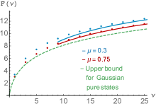
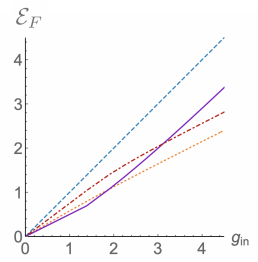
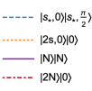
Figure 1: Left: behaviour of the right hand side of (4) as a function of $\nu=N/n_{A}$, for different values of $\mu=n_{A}/n_{B}$, as indicated. The dots are obtained from numerical solutions of (3) ($n_{A}=3$). Full lines are computed using (8) for large $N$. The green dashed line represents the Gaussian bound in (10).
Right: $\mathcal{E}_{F}({\psi_{\textrm{out}}})$ at the output of a beam splitter as a function of $g_{in}=g(\frac{1}{2}({{\mathcal{M}}_{\textrm{TN}}}({\psi_{\textrm{in}}})-1))$ for various $|{\psi_{\textrm{in}}}\rangle$, as indicated. $|2s,0\rangle|0\rangle$ and $|s_{*},0\rangle|s_{*},\frac{\pi}{2}\rangle$ are squeezed states with the same ${{\mathcal{M}}_{\textrm{TN}}}({\psi_{\textrm{in}}})=\cosh(2s_{*})$ ($s=\frac{1}{4}\cosh^{-1}(2\cosh(2s_{*})-1)$). The Fock states $|N\rangle|N\rangle$ and $|2N\rangle|0\rangle$ also have the same ${{\mathcal{M}}_{\textrm{TN}}}({\psi_{\textrm{in}}})=2N+1$.

III Entanglement generation with a beam splitter.

It is well known that a balanced beam splitter $\hat{B}=~{}\exp(\frac{\pi}{4}(a_{1}^{\dagger}a_{2}-~{}a_{1}a_{2}^{\dagger}))$ applied to a separable in-state $|\psi_{\textrm{in}}\rangle$ produces an out-state $|\psi_{\textrm{out}}\rangle=\hat{B}|\psi_{\textrm{in}}\rangle$ that can be entangled provided the in-state is optically nonclassical Kim et al. (2002); Xiang-bin (2002); Asbóth et al. (2005); Killoran et al. (2016). In Asbóth et al. (2005) this property is used to quantify the amount of nonclassicality in a single-mode state $|\varphi\rangle$ by the amount of entanglement obtained in the out-state of a balanced beam splitter with as input state $|\psi_{\textrm{in}}\rangle=|\varphi\rangle\otimes|0\rangle$. Here we take a different approach. We treat entanglement and optical nonclassicality as independently and a priori defined properties of the states, and bound the amount of entanglement that can be obtained in the out-state by the amount of nonclassicality of a general separable in-state, as measured by its ${{\mathcal{M}}_{\textrm{TN}}}$. By applying Theorem 1, we are indeed able to determine how efficiently a beam splitter can generate entanglement in this manner. To see this, note that Eq. (5) implies an upper bound on the entanglement of formation of $|\psi_{\textrm{out}}\rangle$ given the amount of optical nonclassicality available in $|\psi_{\textrm{in}}\rangle$, as follows. Let, for any value of the available nonclassicality ${{{\mathcal{M}}_{\textrm{TN}}}}_{,0}>0$,

$$S_{0}=\{|{\psi_{\textrm{in}}}\rangle=|\varphi_{A},\varphi_{B}\rangle\,\,|\,\,{{\mathcal{M}}_{\textrm{TN}}}({\psi_{\textrm{in}}})\leq{{\mathcal{M}}_{\textrm{TN}}}_{,0}\}.$$

Since $\hat{B}$ preserves the total noise (${\mathcal{N}}_{\textrm{tot}}({\psi_{\textrm{out}}})={\mathcal{N}}_{\textrm{tot}}({\psi_{\textrm{in}}})$), Eq. (5) implies

$$\mathcal{E}_{F}({\psi_{\textrm{out}}})\leq g\left(\frac{1}{2}({{\mathcal{M}}_{\textrm{TN}}}({\psi_{\textrm{in}}})-1)\right)\leq g(\frac{1}{2}({{\mathcal{M}}_{\textrm{TN}}}_{,0}-1)),$$

since $g$ is a monotonically increasing function. To see the bound is reached, let, for $s\geq 0,\phi\in[0,2\pi[$, $S(s,\phi)=e^{\frac{s}{2}(e^{-i\phi}a^{2}-e^{i\phi}a^{{\dagger}2})}$ and define $|\varphi_{A}\rangle=|s_{0},0\rangle:=S(s_{0},0)|0\rangle$ and $|\varphi_{B}\rangle=|s_{0},\pi/2\rangle:=S(s_{0},\frac{\pi}{2})|0\rangle$, with $s_{0}$ chosen so that ${{\mathcal{M}}_{\textrm{TN}}}({\psi_{\textrm{in}}})=\cosh(2s_{0})={{\mathcal{M}}_{\textrm{TN}}}_{,0}$. In this case, $|{\psi_{\textrm{out}}}\rangle$ $=\hat{B}|{\psi_{\textrm{in}}}\rangle=|\psi_{\textrm{TMS}}\rangle$, where $|\psi_{\textrm{TMS}}\rangle$ is the two-mode squeezed vacuum state with ${{\mathcal{M}}_{\textrm{TN}}}(\psi_{\textrm{TMS}})={{\mathcal{M}}_{\textrm{TN}}}_{,0}$, which we saw saturates (5). There is a readily identified family of states that saturate the bound (see Appendix A), but typically states in $S_{0}$ do not. Several physically interesting examples are given in Fig. 1; see Appendix D for details on the computations. When $|{\psi_{\textrm{in}}}\rangle=|N,0\rangle$, ${{\mathcal{M}}_{\textrm{TN}}}({\psi_{\textrm{in}}})=N+1$ and the entanglement of formation of the out-state satisfies $\mathcal{E}_{F}({\psi_{\textrm{out}}})/g(\frac{1}{2}({{\mathcal{M}}_{\textrm{TN}}}({\psi_{\textrm{in}}})-1))\simeq\frac{1}{2}$ for large $N$. Hence, only one half of the possible maximal amount of entanglement is produced in this manner for a given amount of optical nonclassicality in the in-state. When $|{\psi_{\textrm{in}}}\rangle=|N,N\rangle$, on the other hand, ${{\mathcal{M}}_{\textrm{TN}}}({\psi_{\textrm{in}}})=2N+1$, and, for large $N$, the entanglement of formation satisfies $\mathcal{E}_{F}({\psi_{\textrm{out}}})/g(\frac{1}{2}({{\mathcal{M}}_{\textrm{TN}}}({\psi_{\textrm{in}}})-1))\simeq 1$, hence almost the maximum possible amount of entanglement is produced. It is therefore less efficient to input a $2N$ photon state on one mode and the vacuum on the other, rather than $N$ photons on each. A similar phenomenon occurs with squeezed states at the input: $|{\psi_{\textrm{in}}}\rangle=|2s,0\rangle|0\rangle$ and $|{\psi_{\textrm{in}}}\rangle=|s_{*},0\rangle|s_{*},\frac{\pi}{2}\rangle$ with $s=\frac{1}{4}\cosh^{-1}(2\cosh(2s_{*})-1)$ have the same values of ${{\mathcal{M}}_{\textrm{TN}}}=\cosh(2s_{*})$, but the output $\mathcal{E}_{F}$ is, for large $N$, twice as large in the second case.

Let us point out that, in terms of resource theory, the beam splitter does not “convert” nonclassicality into entanglement. Indeed, the total noise is conserved and none of the optical nonclassicality resource is lost in the process. Nevertheless, the above bounds imply that the in-state must have a large amount of optical nonclassicality for the entanglement production to be efficient in this manner. Now note that it was shown in Hertz and De Bièvre (2020) that environmental coupling leads to nonclassicality loss on a time scale inversely proportional to the ${{\mathcal{M}}_{\textrm{TN}}}$ of a pure state such as $|\psi_{\textrm{in}}\rangle$: this implies that strongly nonclassical states $|\psi_{\textrm{in}}\rangle$ with a large ${{\mathcal{M}}_{\textrm{TN}}}$ are hard to maintain, so that the production of strongly entangled states with the above procedure will be difficult to realize.

As mentioned above, Theorems 1 and 1’ involve convex roofs, which are hard to exploit for mixed states. This is true even for Gaussian states, for which the entanglement of formation remains difficult to evaluate, despite recent progress Tserkis and Ralph (2017); Tserkis et al. (2019). This problem can, however, be overcome by using alternative, computable measures of entanglement and optical nonclassicality adapted to Gaussian states.

IV Gaussian states: bounding ${\mathcal{E}_{\mathcal{N}}}$ by ${\mathcal{C}}$.

Consider a Gaussian state $\rho_{\textrm{G}}$ with covariance matrix as defined in (11). We will evaluate its nonclassicality using two recently introduced and readily computable quantities: the total quantum Fisher information ($\mathcal{F}_{\text{tot}}$) (see (12)) and the quadrature coherence scale (${\mathcal{C}}$) (see (14)). We recall that the set of optical classical states ${\mathcal{C}}_{\textrm{cl}}$ Titulaer and Glauber (1965) of a system of $n$ modes contains all mixtures of coherent states $D(\alpha)|0\rangle$, where $D(\alpha)=\exp(\alpha a^{\dagger}-\alpha^{*}a)$ $[\alpha=(\alpha_{1},\alpha_{2},\dots,\alpha_{n})\in\mathbb{C}^{n}\text{ and }a=(a_{1},a_{2},\cdots,a_{n})]$ is the displacement operator and $|0\rangle$ is the $n$-mode vacuum.

For any state $\rho$ and observable $A$, the quantum Fisher information of $\rho$ for $A$ is $\mathcal{F}(\rho,A)=4\partial_{x}^{2}D_{B}^{2}(\rho,\exp(-ixA)\rho\exp(ixA))_{|x=0},$ where $D_{B}^{2}(\rho,\sigma)=2(1-F(\rho,\sigma))$ is the Bures distance and $F(\rho,\sigma)=\operatorname{Tr}\sqrt{\sqrt{\rho}\sigma\sqrt{\rho}}$ the fidelity between $\rho$ and $\sigma$. It is known that $\mathcal{F}(\rho,A)$ is convex in $\rho$ and coincides with $4\,\Delta A^{2}$ on pure states Tóth and Petz (2013); Yu (2013). The total quantum Fisher information of an $n$-mode state $\rho$ is defined as

$$\mathcal{F}_{\textrm{tot}}(\rho)=\frac{1}{4n}\sum_{j=1}^{2n}\mathcal{F}(\rho,{\mathbf{R}}_{j}).$$ (12)

It follows that $\mathcal{F}_{\text{tot}}(\psi)$ coincides with ${{\mathcal{M}}_{\textrm{TN}}}(\psi)$ on pure states, and, since it is convex, ${\mathcal{F}_{\textrm{tot}}}(\rho)\leq{{\mathcal{M}}_{\textrm{TN}}}(\rho)$. It is known that the total quantum Fisher information is a nonclassicality witness, meaning that $\mathcal{F}_{\textrm{tot}}(\rho)>1$ implies $\rho$ is nonclassical De Bièvre et al. (2019). It is however not a nonclassicality measure since there exist nonclassical states for which $\mathcal{F}_{\textrm{tot}}(\rho)\leq 1$. Contrary to ${{\mathcal{M}}_{\textrm{TN}}}$, however, it has the considerable advantage that is can be relatively easily computed on large classes of states. This is in particular true for Gaussian states, where one has Yadin et al. (2018)

$${\mathcal{F}_{\textrm{tot}}}(\rho_{G})=\frac{1}{2n}\mathrm{Tr}V^{-1}.$$ (13)

In De Bièvre et al. (2019); Hertz and De Bièvre (2020) the (squared) quadrature coherence scale is defined as

$${\mathcal{C}}^{2}(\rho)=\frac{1}{2n\mathcal{P}}\left(\sum_{j=1}^{2n}\operatorname{Tr}[\rho,R_{j}][R_{j},\rho]\right),\,\,\,\mathcal{P}=\operatorname{Tr}\rho^{2}.$$ (14)

The quadrature coherence scale measures the spread of the coherences of the quadratures of the state Hertz and De Bièvre (2020). Like the total quantum Fisher information, the quadrature coherence scale is an optical nonclassicality witness: if ${\mathcal{C}}^{2}(\rho)>~{}1$ then $\rho$ is nonclassical De Bièvre et al. (2019). But it is not a nonclassicality measure. It can however serve to construct such a measure, as shown in De Bièvre et al. (2019).

In general, $\mathcal{F}_{\text{tot}}$ and the ${\mathcal{C}}^{2}$ capture different properties of states and can in fact strongly differ on certain states De Bièvre et al. (2019). Nevertheless, they are both nonclassicality witnesses, and coincide on pure states:

$${\mathcal{C}}^{2}(\psi)={\mathcal{F}_{\textrm{tot}}}(\psi)={{\mathcal{M}}_{\textrm{TN}}}(\psi)=\frac{1}{n}{\mathcal{N}}_{\textrm{tot}}(\psi).$$ (15)

In addition, as we now show, they coincide on all Gaussian states as well, including mixed ones:

$${\mathcal{C}}^{2}(\rho_{\textrm{G}})={\mathcal{F}_{\textrm{tot}}}(\rho_{\textrm{G}})=\frac{1}{2n}\mathrm{Tr}V^{-1}.$$ (16)

In view of Eq. (13), it only remains to prove the first equality. We first note that, since both ${\mathcal{C}}(\rho_{\textrm{G}})$ and ${\mathcal{F}_{\textrm{tot}}}(\rho_{\textrm{G}})$ are invariant under phase space translations, we can assume that $\langle R_{i}\rangle=0$ for all $i$. The characteristic function of $\rho_{G}$ is

$$\chi_{G}(\xi)=\mathrm{Tr}\rho_{G}D(\xi)=\exp\{-\frac{1}{2}\xi^{T}\Omega V\Omega^{T}\xi\},$$

$$\text{where}\quad\Omega=\bigoplus_{k=1}^{n}\begin{pmatrix}0&1\\ -1&0\end{pmatrix},$$

and $\xi=(\xi_{11},\xi_{12},\cdots,\xi_{n1},\xi_{n2})$. It was shown in  Gu (1990); De Bièvre et al. (2019) that the right hand side of (14) can be written in terms of the characteristic function $\chi(\xi)$ of the state as follows:

$${\mathcal{C}}^{2}(\rho)=\frac{\||\xi|\chi\|_{2}^{2}}{n\|\chi\|_{2}^{2}}.$$ (17)

Here $\|\cdot\|_{2}$ designates the $L^{2}$-norm, (for example $\|\chi\|_{2}^{2}:=\int|\chi|^{2}(\xi){\mathrm{d}}^{2}\xi$). From (17), one finds with a direct computation

$${\mathcal{C}}^{2}(\rho_{G}) = \frac{1}{n}\int\left(|\xi_{1}|^{2}+\cdots+|\xi_{n}|^{2}\right)f(\xi){\mathrm{d}}^{2}\xi$$

$$= \frac{1}{n}\mathrm{Tr}\Sigma=\frac{1}{2n}\mathrm{Tr}V^{-1}$$

where $f(\xi)$ is a Gaussian probability density with 0 mean value and covariance matrix $\Sigma=\frac{1}{2}\Omega V^{-1}\Omega^{T}$.

We will now connect the optical nonclassicality of Gaussian states (measured with $\mathcal{F}_{\text{tot}}$, or equivalently ${\mathcal{C}}^{2}$) to their entanglement, measured with the logarithmic negativity ${\mathcal{E}_{\mathcal{N}}}$ Vidal and Werner (2002). Let $\mathcal{T}_{B}$ stand for partial transposition in Fock basis applied to the $n_{B}$ modes only, so that $\tilde{\rho}=\mathcal{T}_{B}[\rho]$ denotes the partial transpose of an arbitrary state $\rho$. It is known that if $\tilde{\rho}$ is not positive semidefinite, then $\rho$ is entangled Peres (1996). For a bi-partite system of $n_{A}+n_{B}=n$ modes, the logarithmic negativity of $\rho$ is then defined as ${\mathcal{E}_{\mathcal{N}}}(\rho)=\ln(\operatorname{Tr}\sqrt{\tilde{\rho}^{2}})$. Note that ${\mathcal{E}_{\mathcal{N}}}(\rho)>~{}0$ implies that $\rho$ is entangled. For pure states, but not in general, one has $\mathcal{E}_{F}(|\psi\rangle\langle\psi|)\leq{\mathcal{E}_{\mathcal{N}}}(|\psi\rangle\langle\psi|)$ Vidal and Werner (2002). The partial transpose $\tilde{\rho}_{G}$ of a Gaussian state is again a Gaussian operator, with covariance matrix $\tilde{V}=T_{B}VT_{B}$, where $T_{B}={\mathbb{I}}_{2n_{A}}\bigoplus_{k=1}^{n_{B}}\begin{pmatrix}1&0\\ 0&-1\end{pmatrix}$. The logarithmic negativity of an arbitrary Gaussian state can be expressed in terms of the symplectic spectrum $\tilde{\nu}_{-,1}\leq\dots\leq\tilde{\nu}_{-,n_{-}}<1\leq\tilde{\nu}_{+,1}\leq\dots\leq\tilde{\nu}_{+,n_{+}}$ $(n_{-}+n_{+}=n$) of $\tilde{V}$, as follows Vidal and Werner (2002): if $n_{-}=0$, then ${\mathcal{E}_{\mathcal{N}}}(\rho_{\textrm{G}})=0$, otherwise if $n_{-}\geq 1$,

$${\mathcal{E}_{\mathcal{N}}}(\rho_{\textrm{G}})=\sum_{i=1}^{n_{-}}\ln\frac{1}{\tilde{\nu}_{-,i}}.$$

This equation together with Eq. (16) allow us to derive a main bound for arbitrary Gaussian states:

Theorem 2

Let $\rho_{G}$ be a bipartite Gaussian state, then

$${\mathcal{E}_{\mathcal{N}}}(\rho_{\textrm{G}})\leq n_{-}\left(\ln{\mathcal{C}}^{2}(\rho_{G})+\ln\frac{n}{n_{-}}\right).$$ (18)

Proof.

We note that $\tilde{V}^{-1}=T_{B}V^{-1}T_{B}$ so that ${\mathcal{C}}^{2}(\rho_{G})=\frac{1}{2n}\mathrm{Tr}\tilde{V}^{-1}$. Therefore,

$${\mathcal{C}}^{2}(\rho_{G})\geq\frac{1}{2n}\mathrm{Str}\tilde{V}^{-1} = \frac{1}{n}\left(\sum_{i=1}^{n_{-}}\frac{1}{\tilde{\nu}_{-,i}}+\sum_{i=1}^{n_{+}}\frac{1}{\tilde{\nu}_{+,i}}\right)$$

$$\geq \frac{1}{n}\sum_{i=1}^{n_{-}}\frac{1}{\tilde{\nu}_{-,i}}$$

since $\mathrm{Tr}A\geq\mathrm{Str}A$ Bhatia and Jain (2015) and since $\tilde{\nu}_{+,i}\geq 0$, $\forall i$. Using the concavity of the logarithm, it implies (18). ∎

In the special case $n_{A}=n_{B}=1$, a better bound can be obtained when ${\mathcal{E}_{\mathcal{N}}}(\rho_{\textrm{G}})>0$ using the knowledge of $\det V=\det\tilde{V}=\tilde{\nu}_{-}^{2}\tilde{\nu}_{+}^{2}$:

$${\mathcal{C}}^{2}(\rho_{G})\geq\frac{1}{2}\left(\frac{1}{\tilde{\nu}_{-}}+\frac{1}{\tilde{\nu}_{+}}\right)=\frac{1}{2}\left(\frac{1}{\tilde{\nu}_{-}}+\frac{\tilde{\nu}_{-}}{\sqrt{\det V}}\right)$$

with $\tilde{\nu}_{-}={\mathrm{e}}^{-{\mathcal{E}_{\mathcal{N}}}(\rho_{\textrm{G}})}$. This inequality is saturated when the trace and symplectic trace of $\tilde{V}^{-1}$ coincide.

Theorem 2 shows that a large entanglement implies a large optical nonclassicality, but, in contrast with Theorem 1, both sides of the inequality are readily computable. It is instructive to rework (18) and eliminate $n_{-}$ from it:

Corollary 2

Let $\rho_{\textrm{G}}$ be a Gaussian state. Then

$${\mathcal{E}_{\mathcal{N}}}(\rho_{\textrm{G}})>\frac{n}{\mathrm{e}} \ \ \Rightarrow\ \ \ln{\mathcal{C}}^{2}(\rho_{G})\geq\frac{1}{n}{\mathcal{E}_{\mathcal{N}}}(\rho_{\textrm{G}})-\frac{1}{\mathrm{e}},\qquad$$ (19)

$${\mathcal{C}}^{2}(\rho_{G})<{\mathrm{e}}^{-\frac{n}{e}} \ \Rightarrow\ {\mathcal{E}_{\mathcal{N}}}(\rho_{\textrm{G}})=0.$$ (20)

Proof.

First note that $n_{-}\ln(n/n_{-})\leq n/{\mathrm{e}}$, so that (18) implies $n_{-}\ln{\mathcal{C}}^{2}(\rho_{G})\geq{\mathcal{E}_{\mathcal{N}}}(\rho_{\textrm{G}})-\frac{n}{\mathrm{e}}.$ Hence, if ${\mathcal{E}_{\mathcal{N}}}(\rho_{\textrm{G}})-\frac{n}{\mathrm{e}}>0$, then $n_{-}\geq 1$ and ${\mathcal{C}}^{2}(\rho_{G})>1$. Equation (19)) then follows.

To prove (20), note that (18) implies that

$$n_{-}\ln\frac{1}{{\mathcal{C}}^{2}(\rho_{G})} \leq -{\mathcal{E}_{\mathcal{N}}}(\rho_{\textrm{G}})-n\frac{n_{-}}{n}\ln\frac{n_{-}}{n}\leq\frac{n}{e}.$$

Hence ${\mathcal{C}}^{2}(\rho_{\textrm{G}})\geq{\mathrm{e}}^{-\frac{n}{{\mathrm{e}}n_{-}}}$. Therefore, if ${\mathcal{C}}^{2}(\rho_{G})\leq{\mathrm{e}}^{-\frac{n}{e}}$ then $n_{-}<1$ which implies (20). ∎

Estimate (19) provides a precise quantitative meaning to the statement that a strongly entangled Gaussian state has a large ${\mathcal{C}}^{2}(\rho_{\mathrm{G}})$ and is therefore far from optical classicality. One observes here, as in (6), an exponential growth of the optical nonclassicality with the entanglement of $\rho_{\textrm{G}}$. Estimate (20) shows that a Gaussian state with small ${\mathcal{C}}^{2}(\rho_{\mathrm{G}})$ (well below the nonclassicality threshold $1$) cannot be entangled.

V Conclusions.

We have established inequalities relating, for arbitrary states of a multi-mode optical field, several standard measures of entanglement and of optical nonclassicality. In a nutshell, the optical nonclassicality of a strongly entangled state is necessarily large and, in fact, grows exponentially with its entanglement. As an application, we have bounded the amount of entanglement of formation that can be produced by sending a separable pure state through a beam splitter. Our bound implies that the nonclassicality of the in-state needs to be exponentially large as a function of the expected entanglement of formation of the out-state. Since nonclassicality is a resource that is hard to generate and preserve due to environmental decoherence, as shown in Hertz and De Bièvre (2020), our results can be interpreted to say that, inasfar as the states of a multi-mode bosonic quantum field are concerned, the fragility of their entanglement is a consequence of their large nonclassicality. In addition, we have shown that entanglement is more efficiently produced in a beam splitter when the nonclassicality is distributed equally among the two input modes.

Measuring entanglement or nonclassicality is, in general, a difficult task, but, by restricting to Gaussian states (including mixed ones), we also have established bounds between explicitly computable measures. In the process, we have derived an explicit and simple formula for the quadrature coherence scale of a Gaussian state which only depends on the covariance matrix.

Finally, let us mention that there is interest in comparing the nonclassicality and entanglement of multimode (non-Gaussian) states, for example of the photon added and subtracted states Walschaers et al. (2017); Ra et al. (2020). The tools developed in this paper can serve this purpose.

Appendix A States saturating the bound (5)

We identify here all pure states $|\psi\rangle$ of $n$ modes that saturate (5) with $n_{A}=n_{B}=\frac{n}{2}$; $n$ is even. Let us write

$$|\psi\rangle=\sum_{k,l}c_{k,l}|k,l\rangle,\quad\sum_{k,l}|c_{k,l}|^{2}=1,$$ (21)

with $k=(k_{1},\dots,k_{n_{A}}),l=(l_{1},\dots,l_{n_{A}})\in{\mathbb{N}}^{n_{A}}$. The reduced states on the first (or last) $n_{A}$ modes are

$$\rho_{A}=\sum_{k,k^{\prime}}\left(CC^{\dagger}\right)_{k,k^{\prime}}|k\rangle\langle k^{\prime}|,\qquad\rho_{B}=\sum_{l,l^{\prime}}\left(C^{\dagger}C\right)_{l,l^{\prime}}|l\rangle\langle l^{\prime}|,$$

where $C$ is the operator defined as $C=\sum_{k,k^{\prime}}c_{k,k^{\prime}}|k\rangle\langle k^{\prime}|$ and we use the notation $(\cdot)_{k,k^{\prime}}=\langle k|\cdot|k^{\prime}\rangle$. The right hand side of (5) is the von Neumann entropy of the unique thermal state $\rho_{\beta}$ of $n_{A}$ modes, determined by $\rho_{\beta}=Z_{\beta}^{-1}\sum_{k}{\mathrm{e}}^{-\beta|k|_{1}}|k\rangle\langle k|,$ with $|k|_{1}=\sum_{i=1}^{n_{A}}k_{i}$, where $\beta$ is chosen such that $\operatorname{Tr}\hat{N}_{A}\rho_{\beta}=\frac{n_{A}}{e^{\beta}-1}=\frac{N}{2}.$ The bound is therefore saturated iff $\rho_{A}=\rho_{B}=\rho_{\beta}$, and hence iff $C^{\dagger}C=CC^{\dagger}=D$, with $D$ being a diagonal operator with entries $d_{k}=~{}Z_{\beta}^{-1}{\mathrm{e}}^{-\beta|k|_{1}}$. Let $U=CD^{-1/2}$, then $U$ is unitary and, with $C=UD^{1/2}$, one finds $D=CC^{\dagger}=UDU^{\dagger}\ \Leftrightarrow\ DU=UD.$ We conclude that $|\psi\rangle$ in (21) saturates the bound iff $C=UD^{1/2}$, with $U$ being a unitary operator commuting with $D$. One obvious choice is to take $U={\mathbb{I}}$, in which case $|\psi\rangle$ is an $n/2$-fold tensor product of two-mode squeezed states

$$|\psi_{\textrm{TMS}}\rangle=\cosh(r)^{-1}\sum_{k=0}^{+\infty}(\tanh r)^{k}|k,k\rangle,\quad\beta=\ln\coth^{2}(r)$$

for which ${{\mathcal{M}}_{\textrm{TN}}}(\psi_{\textrm{TMS}})=\cosh(2r)$ and $\mathcal{E}_{F}(\psi_{\textrm{TMS}})=g(\sinh^{2}(r))$. Thus, $|\psi\rangle$ is a Gaussian state with ${{\mathcal{M}}_{\textrm{TN}}}(\psi)=\cosh(2r)$ and $\mathcal{E}_{F}(\psi)=\frac{n}{2}\,g(\sinh^{2}(r))$, saturating the bound (5).

Note that this is not the unique state saturating the bound since such a state is determined by $C=UD^{1/2}=D^{1/2}U$, with $U$ unitary. Therefore, all saturating states can be obtained from the above choice by applying local unitaries $U_{A}$ and $U_{B}$ that preserve the photon numbers $\hat{N}_{A}$ and $\hat{N}_{B}$, setting $C=U_{A}D^{1/2}U_{B}$. For example, when $n=2$, they are all states of the form

$$|\psi\rangle=\cosh(r)^{-1}\sum_{k=0}^{+\infty}(\tanh r)^{k}\exp(i\phi_{k})|k,k\rangle$$

with arbitrary phases $\phi_{k}$. If $\phi_{k}=k\phi$, these states are the general two-mode squeezed states obtained when we inject two orthogonal squeezed states in a balanced beam splitter, the angle of the squeezing of the first input state being $\phi$ (the second input state is squeezed along $\phi+\pi/2$). For general $n$, one has

$$|\psi\rangle=Z_{\beta}^{-1/2}\sum_{k}\exp(-\beta|k|_{1}/2)|\varphi_{A,k},\varphi_{B,k}\rangle$$

where $|\varphi_{A,k}\rangle=U_{A}|k\rangle$, $|\varphi_{B,k}\rangle=U_{B}|k\rangle$ and $Z_{\beta}^{-1/2}$ is a normalization constant; note that $\hat{N}_{A}|\varphi_{A,k}\rangle=|k|_{1}|\varphi_{A,k}\rangle,$ and $\hat{N}_{B}|\varphi_{B,k}\rangle=|k|_{1}|\varphi_{B,k}\rangle.$ In general, such states are not Gaussian.

Appendix B Proof of (8)

We prove here the asymptotic expression for $N_{A}^{*}(N)$, namely Eq. (8). We rewrite Eq. (3) as

$$\mu g(\nu_{*})=g(\mu(\nu-\nu_{*})),$$ (22)

where $\nu_{*}=N_{A}^{*}/n_{A}$, $\mu=n_{A}/n_{B}$, and $\nu=N/n_{A}$. Since we are mostly interested in states with a large optical nonclassicality, we consider the case where $\nu\gg 1$. Writing $\nu_{*}/\nu=1-\delta$ and using that for large $x$, $g(x)\simeq\ln({\mathrm{e}}x)+\frac{1}{2x}$, Eq. (22) becomes

$$\mu\ln({\mathrm{e}}\nu(1-\delta))+\frac{\mu}{2\nu(1-\delta)}=\ln({\mathrm{e}}\mu\nu\delta)+\frac{1}{2\mu\nu\delta}.$$

Suppose now that $\delta\ll 1$, $\mu\nu\delta\gg 1$, and $\nu(1-\delta)\gg 1$. Then, we find

$$N_{A}^{*} = (1-\delta)N,\$$ (23)

$$\textrm{with}\ \ \ \delta = \frac{1}{\mu}\left[1-\frac{{\mathrm{e}}^{1-\mu}}{2\nu^{\mu}}\right]\frac{1}{({\mathrm{e}}\nu)^{1-\mu}+1}.$$

Keeping only the dominant term, one finds (8). In Fig. 2 the numerically computed solution to (22) is compared to the asymptotic expressions (23). The agreement is seen to be excellent, even for relatively small values of $\nu$. The asymptotic expression (8) is also shown for comparison.

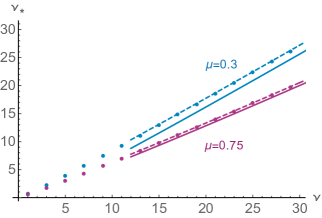
Figure 2: Numerically computed solution $\nu_{*}$ of (22) (dots) and asymptotic expression (8) (plain line) and (23) (dashed line) of $\nu_{*}=N_{A}^{*}/n_{A}$, for different values of $\mu$, as indicated.

Appendix C Non-Gaussian states violating bound (10)

We now show that there exist non Gaussian states that violate the Gaussian bound (10). For that purpose, we consider the case $n_{A}=1,n_{B}=2$. The Gaussian states that saturate the bound are then explicitly given by $(0<~{}q<1)$

$$|\psi_{q}\rangle=(1-q)^{1/2}\sum_{n}q^{n/2}|n;n,0\rangle.$$

Here we wrote $|n;m_{1},m_{2}\rangle$ for the Fock state with $n$ photons in the single $A$ mode and $m_{1}$, respectively $m_{2}$ photons in the two modes of $B$. For this state, we have explicitly $\langle\psi_{q}|\hat{N}|\psi_{q}\rangle=\frac{2q}{1-q}$ and ${{\mathcal{M}}_{\textrm{TN}}}(\psi_{q})=\frac{2}{3}\langle\psi_{q}|\hat{N}|\psi_{q}\rangle+1.$ We will now exhibit a non Gaussian local transformation $U_{B}$ that, when applied to $|\psi_{q}\rangle$, yields a state $|\psi^{\prime}\rangle=U_{B}|\psi_{q}\rangle$ that has the same entanglement of formation as $|\psi_{q}\rangle$ (since $U_{B}$ is local) but that lowers its ${{\mathcal{M}}_{\textrm{TN}}}$. In other words, we will show that

$${{\mathcal{M}}_{\textrm{TN}}}(\psi^{\prime})<{{\mathcal{M}}_{\textrm{TN}}}(\psi_{q}).$$ (24)

This implies that

$$\ \mathcal{E}_{F}(\psi^{\prime})=\mathcal{E}_{F}(\psi_{q})=g(\langle\psi_{q}|\hat{N}|\psi_{q}\rangle/2)>g(\langle\psi^{\prime}|\hat{N}|\psi^{\prime}\rangle/2),\$$

and therefore shows $|\psi^{\prime}\rangle$ does not satisfy the Gaussian bound (10). Of course, it does satisfy the bound (2). The local transformation $U_{B}$ is constructed as follows. Let $k>1$ be fixed. Then

$$U_{B}|m_{1},m_{2}\rangle = |m_{1},m_{2}\rangle,\ \ \textrm{if}\ m_{1}m_{2}\not=0,$$

$$U_{B}|0,0\rangle = |0,0\rangle,$$

$$U_{B}|m_{1},0\rangle = |m_{1},0\rangle,\ \ \textrm{if}\ m_{1}\not=k,$$

$$U_{B}|k,0\rangle = |0,1\rangle,$$

$$U_{B}|0,1\rangle = |k,0\rangle$$

$$U_{B}|0,m_{2}\rangle = |0,m_{2}\rangle,\ \ \textrm{if}\ m_{2}>1.$$

With $|\psi^{\prime}\rangle=U_{B}|\psi_{q}\rangle$ one then easily checks that, for $i=1,2,3$, $\langle\psi^{\prime}|a_{i}|\psi^{\prime}\rangle=0=\langle\psi^{\prime}|a_{i}^{\dagger}|\psi^{\prime}\rangle,$ so that $\langle\psi^{\prime}|X_{i}|\psi^{\prime}\rangle=0=\langle\psi^{\prime}|P_{i}|\psi^{\prime}\rangle$. It follows that ${{\mathcal{M}}_{\textrm{TN}}}(\psi^{\prime})=\frac{2}{3}\langle\psi^{\prime}|\hat{N}|\psi^{\prime}\rangle+1.$ It will therefore suffice to prove $\langle\psi^{\prime}|\hat{N}|\psi^{\prime}\rangle<\langle\psi_{q}|\hat{N}|\psi_{q}\rangle$. One readily finds $\langle\psi^{\prime}|\hat{N}|\psi^{\prime}\rangle=\langle\psi|\hat{N}|\psi\rangle+(1-q)q^{k}(1-k).$ so that (24) follows since $k>1$.

Appendix D Beam splitters

For many states commonly considered the entanglement produced by the beam splitter is considerably lower than the maximal value possible. For example, when $|{\psi_{\textrm{in}}}\rangle=|N,0\rangle$, one obtains

$$|\psi_{\textrm{out}}\rangle=\hat{B}|N,0\rangle=\sum_{m=0}^{N}\sqrt{\frac{n!\,2^{-N}}{m!(N-m)!}}|m,N-m\rangle.$$

Then ${{\mathcal{M}}_{\textrm{TN}}}({\psi_{\textrm{in}}})=N+1$ and $\mathcal{E}_{F}({\psi_{\textrm{out}}})$ is given by the entropy of the binomial distribution $P(k)=\frac{N!}{k!(N-k)!}2^{-N}$, which for large $N$ is approximately given by $\mathcal{E}_{F}({\psi_{\textrm{out}}})\simeq\frac{1}{2}\ln(2\pi{\mathrm{e}}N)$. Hence, in this case, $\mathcal{E}_{F}({\psi_{\textrm{out}}})/g(\frac{1}{2}({{\mathcal{M}}_{\textrm{TN}}}({\psi_{\textrm{in}}})-1))\simeq\frac{1}{2}$, as can be observed in Fig. 1. When $|{\psi_{\textrm{in}}}\rangle=|{N},{N}\rangle$, one has ${{\mathcal{M}}_{\textrm{TN}}}({\psi_{\textrm{in}}})=2N+1$ and Kim et al. (2002)

$$|{\psi_{\textrm{out}}}\rangle=\hat{B}|N,N\rangle=\sum_{m=0}^{N}c_{m}|2m,2N-2m\rangle,$$

$$\text{with}\ \ \ c_{m}=\frac{1}{2^{N}}\frac{\sqrt{(2N-2m)!(2m)!}}{m!(N-m)!}.$$

For large $N$, choosing $m=N/2+\delta$, one can apply the Stirling approximation $N!\rightarrow\sqrt{2\pi N}(N/e)^{N}$ to find that the coefficients $|c_{m}|^{2}$ converge to $\frac{f(m/N)}{N}$ with $f(x)=~{}\frac{1}{\pi}\frac{1}{\sqrt{\frac{m}{N}(1-\frac{m}{N})}}$. This result coincides with the one obtained in Nakazato et al. (2016). The Von Neumann entropy is thus given by

$$-\mathrm{Tr}\rho_{1}\ln\rho_{1} = -\sum_{m=0}^{N}|c_{m}|^{2}\ln|c_{m}|^{2}$$

$$= -\frac{1}{N}\sum_{m=0}^{N}N|c_{m}|^{2}\ln|c_{m}|^{2}$$

$$= -\frac{1}{N}\sum_{m=0}^{N}f(m/N)\ln f(m/N)+\ln N$$

$$\approx -\int_{0}^{1}f(x)\ln f(x)\text{d}x+\ln N$$

$$= \ln\frac{\pi}{4}+\ln N.$$

Hence, in this case $\mathcal{E}_{F}({\psi_{\textrm{out}}})/g(\frac{1}{2}({{\mathcal{M}}_{\textrm{TN}}}({\psi_{\textrm{in}}})-1))\simeq 1$ which means that, asymptotically, the maximal possible amount of entanglement can be produced in this manner. It is therefore more efficient to input a state with $N$ photon on each mode than $2N$ photons on one mode and the vacuum on the other, as in both cases ${{\mathcal{M}}_{\textrm{TN}}}({\psi_{\textrm{in}}})=2N+1$, but the output $\mathcal{E}_{F}$ is, for large $N$, twice as large in the first case.

If $|{\psi_{\textrm{in}}}\rangle=|2s,0\rangle|0\rangle$, one finds the out-state is a two-mode squeezed vacuum state of parameter $s$ on which we add some squeezing $s^{\prime}$ on the first mode and $-s^{\prime}$ on the second. Since those squeezing are local, they do not modify the value of the entanglement of formation, which is thus the one of the two-mode squeezed vacuum state . Hence, $\mathcal{E}_{F}({\psi_{\textrm{out}}})=g(\sinh^{2}(s))$. Note, nevertheless, that while a two-mode squeezed vacuum state of parameter $s$ has a total noise of $\cosh(2s)$, the total noise of the in-state is given by ${{\mathcal{M}}_{\textrm{TN}}}({\psi_{\textrm{in}}})=\frac{\cosh(4s)+1}{2}$. Only about one half of the possible maximal amount of entanglement is produced in this manner. On the other hand, if $|{\psi_{\textrm{in}}}\rangle=|s_{*},0\rangle|s_{*},\frac{\pi}{2}\rangle$, with $s=\frac{1}{4}\cosh^{-1}(2\cosh(2s_{*})-1)\simeq\frac{s_{*}}{2}$ the total noise of the in-state is also given by ${{\mathcal{M}}_{\textrm{TN}}}({\psi_{\textrm{in}}})=\frac{\cosh(4s)+1}{2}$ but yields, after the beam splitter, the maximum entanglement possible, namely $g(\sinh^{2}(s_{*}))\geq g(\sinh^{2}(s))$. So in this instance too it is more efficient, in terms of entanglement creation, to insert a symmetric input in the beam splitter .