Instrumental Variable Estimation of Marginal Structural Mean Models for Time-Varying Treatment

Abstract

Robins (1997b) introduced marginal structural models (MSMs), a general class of counterfactual models for the joint effects of time-varying treatment regimes in complex longitudinal studies subject to time-varying confounding. In his work, identification of MSM parameters is established under a sequential randomization assumption (SRA), which rules out unmeasured confounding of treatment assignment over time. We consider sufficient conditions for identification of the parameters of a subclass, Marginal Structural Mean Models (MSMMs), when sequential randomization fails to hold due to unmeasured confounding, using instead a time-varying instrumental variable. Our identification conditions require that no unobserved confounder predicts compliance type for the time-varying treatment. We describe a simple weighted estimator and examine its finite-sample properties in a simulation study. We apply the proposed estimator to examine the effect of delivery hospital on neonatal survival probability.

Keywords: causal inference, marginal structural model, unmeasured confounding, time-varying endogeneity, delivery hospital

1 Introduction

Robins (1997b, 2000) introduced marginal structural models (MSMs), a class of counterfactual models that encode the joint causal effects of time-varying treatment in the presence of time-varying confounding. For identification, Robins relied on a sequential randomization assumption (SRA), which rules out unmeasured confounding of the time-varying treatment. MSMs have since become the standard analytic approach to evaluate causal effects in time-varying epidemiological studies (Hernán et al., 2002; Morrison et al., 2010; Cerdá et al., 2010; Cook et al., 2002; VanderWeele et al., 2011). However, SRA may be hard to justify in many such settings, and unmeasured confounding bias may invalidate causal claims inferred by the approach. In the case of a point treatment, a large literature in causal inference has developed over the years on the instrumental variable method aiming to address unmeasured confounding Angrist et al. (1996); Baker and Lindeman (1994); Imbens and Angrist (1994); Robins (1994); Heckman and Urzua (2010). Instead of assuming that there is no unmeasured confounding, the IV approach relies on the key assumption that one has observed a pretreatment variable that can affect the outcome only through its effects on the treatment. Many commonly used IVs, such as treatment compliance and tax rates, vary with time. Nevertheless, IV methods in longitudinal settings are far less developed. In this paper, we consider sufficient conditions for identification of the parameters of a Marginal Structural Mean Model (MSMM) with the aid of a time-varying instrumental variable when sequential randomization fails to hold due to time-varying unmeasured confounding. In doing so, we firmly establish the IV approach in the context of MSMMs for complex longitudinal settings, an extension previously believed out of reach Robins (2000). Our identification conditions require longitudinal generalizations of standard IV assumptions, together with a key assumption that no unobserved confounder predicts compliance type for the time-varying treatment, a longitudinal generalization of the identification condition of Wang and Tchetgen Tchetgen (2018). Under these assumptions, we establish identification of the MSMM and propose a simple estimation procedure analogous to inverse-probability weighted (IPW) estimation, the most common approach for estimating MSMs under SRA.

Prior to the current work, Robins (1994) developed a general framework for identification and estimation of causal effects of time-varying endogenous treatments using a time-varying instrumental variable under a structural nested mean model (SNMM). As described in Robins (2000), the parameters of an SNMM can under certain homogeneity conditions be interpreted as MSMM parameters, in which case Robins (1994) provides alternative estimators to ours. In contrast, the proposed methodology is more general as it directly targets MSMM parameters irrespective of whether or not they can be interpreted as parameters of an equivalent SNMM. Robins (1997a) left open the question whether MSMs, like SNMMs, were identifiable by IVs, a question that the current work therefore answers in the affirmative.

The remainder of the paper is organized as follows. In Section 2 we provide context by describing identification and estimation of MSMM parameters under SRA. In Section 3 we present an alternative set of identification conditions to SRA, making use of a time-varying instrumental variable. In Section 4 we establish the necessity of a variation of our key identification condition. In Section 5 we describe a simple weighted estimator for MSMM parameters using our instrumental variable approach. In Section 6 we present a simulation study to examine the finite-sample performance of our proposed estimator. In Section 7, we apply the proposed estimator to examine the effect of delivery hospital on neonatal survival probability. We conclude in Section 8 with a brief discussion and description of future work.

2 Background

We consider i.i.d. discrete-time processes and adopt the “potential outcomes” framework. The data observed on a process consists of $T+2$ random vectors $\overline{L}=(L_{0},\ldots,L_{T+1})$ and $T+1$ random variables $\overline{A}=(A_{0},\ldots,A_{T})$. The common state space of $A_{t},t=1,\ldots,T,$ is denoted $\mathcal{A}$. Variables at time $0$ are defined to be constant, e.g., $A_{0}=0$. The vectors $L_{t}$ and variables $A_{t}$ carry the interpretation of a subject’s time-varying covariates and a time-varying treatment, respectively. A variable $Y\in L_{T+1}$ is singled out as an outcome of interest. The number of time points $T$ is non-random. The statistical significance of these temporal relations are conditional independence relationships formalized in assumptions given below. We use script fonts to refer to state spaces, $f$ to refer to densities, and $\mu$ for measures relative to which densities are given, using subscripts to indicate the law. We use overbars to indicate the history of an RV, e.g., $\overline{L}_{t}=(L_{0},\ldots,L_{t})$. Besides the observed data, we assume the existence of $|\mathcal{A}|^{T}$ variables $Y_{\overline{a}},\overline{a}\in\mathcal{A}^{T}$. These “potential outcomes” or “counterfactuals” are not in general observed. They are related to the observed data by the “consistency” assumption,

Assumption 1 (Consistency).

$Y=Y_{\overline{A}}\hskip 10.03749pt\text{ a.s.}$

In case the treatments $\overline{A}$ are discrete, the assumption may be written as $Y=\sum_{\overline{a}\in\mathcal{A}^{T}}Y_{\overline{a}}\{\overline{A}=\overline{a}\}$, using braces to denote the event indicator. Thus $\overline{a}$ may be interpreted as a particular treatment regime, and the potential outcome $Y_{\overline{a}}$ as the distribution of $Y$ were everyone in the observed population to follow treatment regime $\overline{a}$, i.e., if $\{\overline{A}=\overline{a}\}\equiv 1$.

A marginal structural mean model (“MSMM”) is a model on the marginal means of potential outcomes Robins (1997b). For example, the effect of treatment may be modeled as linear in the cumulative treatment taken,

$$\mathbb{E}(Y_{\overline{a}})=\beta_{0}+\beta_{1}\sum_{t=0}^{T}a_{t}.$$ (1)

In this example, $\beta\in\mathbb{R}^{2}$ parameterizes the model and encodes the incremental effect of a unit of treatment. A link function can be introduced to accommodate binary or count outcome variables, e.g., for binary $Y$, $\mathbb{E}(Y_{\overline{a}})=(1+\exp(\beta_{0}+\beta_{1}\sum_{t=0}^{T}a_{t}))^{-1}.$ In general we write

$$\mathbb{E}(Y_{\overline{a}})=m_{\beta}(\overline{a})$$ (2)

to describe an MSMM, where $m_{\beta}:\mathcal{A}^{T}\to\mathbbm{R}$ belongs to a family of functions parameterized by finite-dimensional $\beta$. The model parameter $\beta$ is the target of inference.

An MSMM is defined using the unobserved quantities $Y_{\overline{a}},\overline{a}\neq\overline{A}$, and the model parameter is not in general identified by the observed data. Robins (1997b) provides sufficient conditions for identification and estimation, the sequential randomization assumption and positivity:

$$Y_{\overline{a}}\perp\!\!\!\perp A_{t}\mid\overline{L}_{t},\overline{A}_{t-1},\quad 1\leq t\leq T\qquad\text{(SRA)}$$ (3)

$$0<f_{A_{t}\mid\overline{A}_{t-1},\overline{L}_{t}}(a_{t}\mid\overline{a}_{t-1},\overline{l}_{t})\text{ when }f_{\overline{A}_{t-1},\overline{L}_{t}}(\overline{a}_{t-1},\overline{l}_{t})>0,\quad a_{t}\in\mathcal{A},1\leq t\leq T,\qquad\text{(positivity)}$$ (4)

using $\perp\!\!\!\perp$ to denote statistical independence. In the treatment setting, SRA will hold if the cumulative observed data at each time point captures all systematic associations between the treatment and outcome of interest. Positivity will hold when, among all subpopulations defined by covariates $\overline{L}_{t}$ and a treatment regime $\overline{A}_{t-1},t\leq T$, there are further subpopulations at each possible treatment level $a_{t}\in\mathcal{A}$. These conditional independence relationships are implied by the causal directed acyclic graph given in Fig. 1, in which a node is independent of non-descendants conditional on its parent nodes; see Richardson and Robins (2013) for details.

Robins (1997b) uses assumptions 3 and 4 to relate the law of a potential outcome $Y_{\overline{a}}$ to the law of the observed data $(Y,\overline{L},\overline{A})$. Specifically, given measurable $g:(\mathcal{Y},\mathcal{A}^{T})\to\mathbbm{R}^{d}$, he established that

$$\int_{\mathcal{A}^{T}}\mathbb{E}\left(g(Y_{\overline{a}},\overline{a})\right)\mu_{\mathcal{A}^{T}}(\overline{a})=\mathbb{E}\left(g(Y,\overline{A})/\overline{W}^{(SRA)}\right),$$ (5)

where the observation weights $1/W^{(SRA)}$ are defined by

$$W^{(SRA)}_{t} =f_{A_{t}\mid\overline{A}_{t-1},\overline{L}_{t}}(A_{t}\mid\overline{A}_{t-1},\overline{L}_{t}),\qquad\overline{W}_{t}^{(SRA)}=\prod_{\tau=1}^{t}W^{(SRA)}_{\tau},\qquad t=1,\ldots,T,$$ (6)

$$\overline{W}^{(SRA)} =\overline{W}_{T}^{(SRA)}=\prod_{\tau=1}^{T}W^{(SRA)}_{\tau}.$$ (7)

This use of overbars to represent the running product of weights departs from our usual use of overbars to denote the history of a time-varying quantity collected in a vector. The case $T=1,g(y,a)=g_{0}(y)\times\mathbbm{1}_{a},$ gives the inverse-probability-weighted estimator for $g_{0}(Y_{a})$ often used in propensity score analysis.

Besides identifying the parameter of an MSMM using fully observed data, relation (5) also suggests an estimator. Let $g(y,\overline{a})=h(\overline{a})(y-m_{\beta}(\overline{a}))$, where $h$ is a function on $\mathcal{A}^{T}$ of the same dimension as $\beta$. Then the MSMM model (2) implies $\mathbb{E}\left(h(\overline{A})\frac{Y-\mu_{\beta}(\overline{A})}{W^{(SRA)}}\right)=\mathbb{E}(h(\overline{a})\left(Y_{\overline{a}}-m_{\beta}(\overline{a})\right))=0$, giving rise to estimating equations for $\beta$,

$$0=\mathbb{P}_{n}\left(h(\overline{A})\frac{Y-\mu_{\hat{\beta}}(\overline{A})}{\overline{W}^{(SRA)}}\right),$$

using $\mathbb{P}_{n}$ to denote the empirical distribution on a sample of size $n$. In practice, $\overline{W}^{(SRA)}$ may not be known and an estimate is substituted. Under standard regularity conditions for M-estimation, the empirical solution $\hat{\beta}$ is asymptotically normal as the number of observations $n$ grows, with a variance that can be approximated by its influence function.

Furthermore, a suitable choice of $h$ in (5) can in some situations provide a means to stabilize the weights (7), which may become unstable as $T$ increases. Stabilized weights are defined as

$$\overline{W}^{(SRA,stabilized)}\coloneqq\prod_{t=1}^{T}f(A_{t}\mid\overline{A}_{t-1})/\overline{W}^{(SRA)}=\prod_{t=1}^{T}f(A_{t}\mid\overline{A}_{t-1})/f(A_{t}\mid\overline{A}_{t-1},\overline{L}_{t}).$$

The quality of the approximation depends on the strength of the dependence of the density of $A_{t}$ and the covariates $\overline{L}_{t}$ given $\overline{A}_{t-1}$, i.e., to the extent that treatment is unconfounded.

We pursue parallel results using instrumental variables to relax SRA. We give an analogue of the identifying relation (5) using IVs in Section 3, and similar estimation techniques in Section 5.

3 Identification of causal model parameters using IVs

Figure 1: Causal DAG describing longitudinal confounding with $T=2$ time points, satisfying SRA.

Figure 2: An example of a causal DAG describing confounding with unobserved confounders and IV, with $T=2$ time points, satisfying the assumptions of Theorem 1. Edges emerging from the IV $Z$ only end at the treatment $A$. The roles of $U$ and $L$ are symmetric except in respect of the IV, with which $L$ but not $U$ is dependent.

We now allow for the possibility of unmeasured confounders in the form of an additional unobserved stochastic process associated with both the treatment and outcome. The sequential randomization assumption (3) is not warranted in this situation. We propose to use “instrumental variables” to identify an MSMM parameter in the absence of SRA. Informally, an IV is a random variable associated with the treatment of interest that only affects the outcome of interest through its effect on the treatment.

To this end, in addition to the data described in Section 2, let $\overline{U}=(U_{1},\ldots,U_{T})$ be an unobserved process, possibly multivariate, which may be associated with both $\overline{A}$ and $\overline{L}$, including $Y$. We assume that $\overline{U}$ captures all further confounding between $\overline{A}$ and $Y$ beyond $\overline{L}$, so that SRA would hold were $\overline{U}$ observed:

Assumption 2 (Latent SRA).

$Y_{\overline{a}}\perp\!\!\!\perp A_{t}\mid\overline{A}_{t-1}=\overline{a}_{t-1},\overline{L}_{t},\overline{U}_{t}\qquad t=1,\ldots,T,\quad\overline{a}\in\mathcal{A}^{T}$

That is, there are no unobserved confounders at time $t$ other than $\overline{U}_{t}$. The assumptions given below impose restrictions on $\overline{U}$.

Suppose further that a binary-valued process $\overline{Z}=(Z_{1},\ldots,Z_{T})$ is observed, satisfying the following IV assumptions: For all $1\leq t\leq T$ and $\overline{a}\in\mathcal{A}^{T},\overline{z}\in\{0,1\}^{T}$,

Assumption 3 (IV relevance).

$\mathbb{E}(A_{t}\mid\overline{A}_{t-1},\overline{L}_{t},\overline{Z}_{t})\neq\mathbb{E}(A_{t}\mid\overline{A}_{t-1},\overline{L}_{t},\overline{Z}_{t-1})$

Assumption 4 (Exclusion restriction).

$Y_{\overline{a}\overline{z}}=Y_{\overline{a}}$

Assumption 5 (IV–outcome independence).

$\overline{Z}_{t}\perp\!\!\!\perp(Y_{\overline{a}},L_{t+1},U_{t+1})\mid\overline{A}_{t}=\overline{a}_{t},\overline{L}_{t},\overline{U}_{t}$

Assumption 6 (IV–unmeasured confounder independence).

$Z_{t}\perp\!\!\!\perp\overline{U}\mid\overline{A}_{t-1},\overline{L}_{t},\overline{Z}_{t-1}$

Assumption 7 (IV Positivity).

$0<\mathbb{P}(Z_{t}=1|\overline{A}_{t-1},\overline{L}_{t},\overline{Z}_{t-1})<1\text{ a.s.}$

Assumptions 3–7 are longitudinal generalizations of standard IV assumptions. As in the SRA case discussed in Section 2, the conditional independence relationships described by the key assumptions 2, 5, and 6, formalize the temporal relationships among the data $A_{t},Y,L_{t}$, etc., that we use informally. A graph that provides a model of these assumptions is given in Fig. 2. The methods given in Richardson and Robins (2013) may be used to establish that the graph in Fig. 2, properly interpreted, does in fact entail a model for the conditional independence relations given in Assumptions 2, 5, and 6. The DAG in Fig. 2 is illustrative and is not meant to preclude other models compatible with these assumptions, e.g., unmeasured confounding among the measured covariates $\{L_{t}\}$ or between $L_{t}$ and the outcome $Y$, analogous to the shaded nodes in Fig. 1. As a shorthand we use the notation “$\operatorname{an}$” to refer to an ancestor set in the DAG in Fig. 2, e.g., $\operatorname{an}(Z_{t})$ is $\operatorname{an}(A_{t-1})\cup\operatorname{an}(Z_{t-1})\cup\operatorname{an}(L_{t})$.

Finally, we make an additional orthogonality assumption. For $t=1,\ldots,T.$

Assumption 8 (Independent Compliance Type).

$$f\left(a_{t}|\overline{A}_{t-1},\overline{Z}_{t-1},Z_{t}=1,\overline{L}_{t},\overline{U}_{t}\right) -f\left(a_{t}|\overline{A}_{t-1},\overline{Z}_{t-1},Z_{t}=0,\overline{L}_{t},\overline{U}_{t}\right)\perp\!\!\!\perp\overline{U}_{t}\mid\overline{A}_{t-1},\overline{Z}_{t-1},\overline{L}_{t}.$$

Defining

$$\Delta_{t}(a_{t},\overline{A}_{t-1},\overline{Z}_{t-1},\overline{L}_{t},\overline{U}_{t})=f\left(a_{t}|\overline{A}_{t-1},\overline{Z}_{t-1},Z_{t}=1,\overline{L}_{t},\overline{U}_{t}\right)-f\left(a_{t}|\overline{A}_{t-1},\overline{Z}_{t-1},Z_{t}=0,\overline{L}_{t},\overline{U}_{t}\right),$$

the assumption is that $\Delta_{t}(a_{t},\overline{A}_{t-1},\overline{Z}_{t-1},\overline{L}_{t},\overline{U}_{t})$ does not depend on $\overline{U}_{t}$, and so may be written as $\Delta_{t}(a_{t},\overline{A}_{t-1},\overline{Z}_{t-1},\overline{L}_{t})$. The function $\Delta_{t}$ may be expressed using the observed data by the relation

$$\Delta_{t}(a_{t},\overline{A}_{t-1},\overline{Z}_{t-1},\overline{L}_{t}) =f\left(a_{t}|\overline{A}_{t-1},\overline{Z}_{t-1},Z_{t}=1,\overline{L}_{t},\overline{U}_{t}\right)-f\left(a_{t}|\overline{A}_{t-1},\overline{Z}_{t-1},Z_{t}=0,\overline{L}_{t},\overline{U}_{t}\right)$$

$$=f\left(a_{t}|\overline{A}_{t-1},\overline{Z}_{t-1},Z_{t}=1,\overline{L}_{t}\right)-f\left(a_{t}|\overline{A}_{t-1},\overline{Z}_{t-1},Z_{t}=0,\overline{L}_{t}\right).$$

The relation follows by integrating both sides of the first line with respect to the conditional density of $\overline{U}_{t}$ given $(\overline{A}_{t},\overline{Z}_{t-1},Z_{t}=1,\overline{L}_{t})$, which is the same as the density given $(\overline{A}_{t},\overline{Z}_{t-1},Z_{t}=0,\overline{L}_{t})$, by Assumption 6.

Assumption 8 states that while $\overline{U}_{t}$ may confound the causal effects of $\overline{A}_{t},$ no component of $\overline{U}_{t}$ interacts with $Z_{t}$ in its additive effects on $A_{t}.$ This assumption is a longitudinal generalization of a similar assumption made by Wang and Tchetgen Tchetgen (2018) in the point exposure setting.

Let $f_{Z_{t}}$ denote the density of $Z_{t}$ conditional on the prior observed history $(\overline{A}_{t-1},\overline{Z}_{t-1},\overline{L}_{t})$, which, by Assumption 6, has the same effect as conditioning on the full prior history $(\overline{A}_{t-1},\overline{Z}_{t-1},\overline{L}_{t},\overline{U}_{t})$. We define subject-specific weights $1/\overline{W}$ through:

$$\overline{W}=\prod_{t=1}^{T}W_{t},\qquad W_{t}=(-1)^{1-Z_{t}}f_{Z_{t}}\left(Z_{t}\mid\overline{L}_{t},\overline{A}_{t-1},\overline{Z}_{t-1}\right)\Delta_{t}\left(\overline{L}_{t},\overline{A}_{t-1},\overline{Z}_{t-1}\right).$$ (8)

Assumptions 3 and 7 ensure that the weights are nonzero.

Theorem 1.

Suppose that together with consistency (1), Assumptions (2–8) hold. For measurable $g:(\mathcal{Y},\mathcal{A}^{T})\to\mathbbm{R}^{d}$,

$$\mathbb{E}\left(g(Y,\overline{A})/\overline{W}\right) =\int_{\mathcal{A}^{T}}g(Y_{\overline{a}},\overline{a})\mu_{\overline{A}^{T}}(\overline{a}),$$ (9)

when the expectation exists.

Proofs are given in the appendix.

Remark 2.

The conclusion of the theorem for the particular choice $g(y,\overline{a})=h(\overline{a})(y-m(a)),h\in L_{1}(\overline{A})$, i.e.,

$$\mathbb{E}\left(h(\overline{A})(Y-m(\overline{A}))/\overline{W}\right)=\int_{\mathcal{A}^{T}}h(\overline{A})(Y_{\overline{A}}-m(\overline{A}))\mu_{\overline{A}^{T}}(\overline{a}),$$ (10)

may be established under weaker forms of Assumptions 1 and 2. Assumption 1 may be replaced with

Assumption 1^′.

$\mathbb{E}(Y\mid\overline{A}_{t}=\overline{a}_{t},\overline{Z}_{t},\overline{L}_{t},\overline{U}_{t})=\mathbb{E}(Y_{\overline{a}}\mid\overline{A}_{t}=\overline{a}_{t},\overline{Z}_{t},\overline{L}_{t},\overline{U}_{t})$,

and Assumption 2 may be replaced with

Assumption 2^′.

$\mathbb{E}(Y_{\overline{a}}\mid\overline{A}_{t}=\overline{a}_{t},\overline{Z}_{t-1},\overline{L}_{t},\overline{U}_{t})=\mathbb{E}(Y_{\overline{a}}\mid\overline{A}_{t-1}=\overline{a}_{t-1},\overline{Z}_{t-1},\overline{L}_{t},\overline{U}_{t})$,

where $\qquad t=1,\ldots,T,\quad\overline{a}\in\mathcal{A}^{T}.$

As the range of $\overline{W}$ includes negative values, $1/\overline{W}$ are not weights in the usual sense, a phenomenon that also occurs in other IV-weighted moment equations for point exposure Wang and Tchetgen Tchetgen (2018); Abadie (2003). The weights in fact have mean zero, as follows by taking expectations on both sides of

$$\mathbb{E}(\overline{W}_{T}^{-1}\mid\operatorname{an}(Z_{T}))=\overline{W}_{T-1}^{-1}\Delta_{T}^{-1}\mathbb{E}\left(\frac{(-1)^{1-Z_{T}}}{f_{Z_{T}}(Z_{T}\mid\overline{A}_{T-1},{Z}_{T-1},\overline{L}_{T})}\bigg{|}\operatorname{an}(Z_{T})\right)=\overline{W}_{T-1}^{-1}\Delta_{T}^{-1}(1-1),$$

although, as mentioned previously, they are almost surely non-zero under the assumptions for identification.

Example 3 (Binary treatment).

Assumption 8 may, in some situations, be interpreted as a condition on the “compliance types” Angrist et al. (1996) of the population.

When the treatment is binary, $A_{t}\in\{0,1\},t=1,\ldots,T$, so that $P(A_{t}=0\mid\operatorname{an}(A_{t}))=1-P(A_{t}=1\mid\operatorname{an}(A_{t}))$, the differences $\Delta_{t}$ satisfy $\Delta_{t}(A_{t}=1)=-\Delta_{t}(A_{t}=0),t=1,\ldots,T$. Consider an application in which $Z_{t}$ indicates whether a subject has been assigned to take an experimental or control treatment at time $t$ and $A_{t}$ indicates whether the assigned treatment was or was not in fact taken. Then $0<\Delta(A_{t}=1)=P(A_{t}=1\mid\operatorname{an}(A_{t}),Z_{t}=1)-P(A_{t}=1\mid\operatorname{an}(A_{t}),Z=0)=P(A_{t}=0\mid\operatorname{an}(A_{t}),Z=0)-P(A_{t}=0\mid\operatorname{an}(A_{t}),Z=1)$ has the interpretation that $A_{t}$ must concord with the IV $Z_{t}$, in the sense that individuals at stratum $\operatorname{an}(A_{t},Z_{t})$ are more likely at time $t$ to take the treatment when assigned to do so than when assigned not to do so. Analogously, when $\Delta(A_{t}=1)<0$, individuals at stratum $\operatorname{an}(A_{t},Z_{t})$ are more likely to do the opposite of their assignment.

An additional assumption leads to an interpretation in terms of a well-studied causal notion, the compliance type. As with the treatment-indexed potential outcomes $Y_{a}$ defined earlier, IV-indexed potential treatments may also be defined, which we denote as $A_{t,Z_{t}}$. These potential outcomes may be cross-classified by the four possible pairs of values of $A_{t,Z_{t}}$ and $Z_{t}$. Experimental subjects for whom $A_{t,Z_{t}=1}=1$ and $A_{t,Z_{t}=0}=0$ are termed “compliers,” as they comply with the assignment $Z_{t}$, and similarly for “defiers,” $A_{t,Z_{t}=1}-A_{t,Z_{t}=0}<0$, “never-takers”, $A_{t,Z_{t}=0}=A_{t,Z_{t}=1}=0$, and “always-takers,” $A_{t,Z_{t}=0}=A_{t,Z_{t}=1}=1$. Suppose that, analogous to SRA, these potential outcomes are conditionally independent of the IV,

$$Z_{t}\perp\!\!\!\perp A_{t,Z_{t}}\mid\overline{U}_{t},\overline{L}_{t},\overline{A}_{t-1},\overline{Z}_{t-1}.$$

Then Assumption 8 asserts that, at each stratum $\operatorname{an}(A_{t},Z_{t})$, the compliance type is mean-independent of unknown confounders,

$$\mathbb{E}\left(A_{t,z_{t}=1}-A_{t,z_{t}=0}|\overline{U}_{t},\overline{L}_{t},\overline{A}_{t-1},\overline{Z}_{t-1}\right)=\Delta_{t}\left(\overline{L}_{t},\overline{A}_{t-1},\overline{Z}_{t-1}\right)\text{, }t=0,...,T-1.$$

Under this interpretation, the inequalities $\Delta(A_{t}=1)>0$ or $\Delta(A_{t}=1)<0$ assert that a given stratum consists only of compliers or defiers. In any event, whether or not this interpretation is available, a population stratum cannot consist of never-takers or always-takers due to Assumption 3. In this application, therefore, Assumption 8 is warranted when enough data on the patients are obtained to account for any systematic differences in compliance type.

Example 4 (Continuous treatment).

We consider the implications of Assumption 8 for continuous treatment densities. First, because $f_{A_{t}\mid\operatorname{an}(A_{t})}(a_{t},Z_{t}=1)$ and $f_{A_{t}\mid\operatorname{an}(A_{t})}(a_{t},Z_{t}=0)$ both integrate to 1 with respect to $\mu_{A_{t}}$, their difference $\Delta_{t}(a_{t})$ must integrate to 0. As the densities vanish at infinity, so must $\Delta_{t}$. As discussed in Section 5, IV estimators are typically unstable when the magnitude of $\Delta_{t}$ is small, and therefore the tails must decay quickly for good performance. Second, $\Delta_{t}$ must be nonzero almost surely with respect to $\mu_{A_{t}}$, by Assumption 7. Third, the nonnegativity of $f_{A_{t}\mid\operatorname{an}(A_{t})}(a_{t},Z_{t}=1)$ requires, for all $U_{t}$, that $|\Delta_{t}(a_{t})|\leq f_{A_{t}\mid\operatorname{an}(A_{t})}(a_{t},Z_{t}=0)$ for $a$ such that $\Delta_{t}(a_{t})<0$. The first two requirements hold for the difference of any two densities that are unequal a.s.$-\mu_{A_{t}}$, but the last is not as easily satisfied. It requires that for a range of densities obtained by varying $U_{t}$, adding $\Delta_{t}$ doesn’t lead to a function that has negative values.

An example is a location-scale parametrization for the treatment density. Let the baseline density $f_{A_{t}\mid\operatorname{an}(A_{t})}(A_{t}=a,L_{t}=(l_{1},l_{2}),U_{t}=u,Z_{t}=0)$ be normal $\phi((a-l_{1})/u)/u$. The first component of the observed confounder $L_{t}$ controls the location and the unobserved confounder $U_{t}$ controls the spread. Let $\Delta_{t}(a\mid L_{t}=(l_{1},l_{2}))$ be a difference between normal densities that does not depend on $U_{t}$, say, $\phi(a)-\phi(a/l_{2})/l_{2}$. If the spread $u$ of the baseline density lies within an appropriate range, then $f_{A_{t}\mid\operatorname{an}(A_{t})}(A_{t}=a,L_{t}=(l_{1},l_{2}),U_{t}=u,Z_{t}=0)+\Delta_{t}(a)$ is a valid density for $A_{t}$. In particular, given $L_{t}=(l_{1},l_{2})$ with $l_{2}\in(0,1)$, suppose $l_{2}<u<\min(1,l_{2}/(1-l)2))$ for the standard deviation $u$ of the baseline. Let $l_{1}=0$ since the location is irrelevant to the argument. Then, as shown in Appendix 10,

$$f_{A_{t}\mid\operatorname{an}(A_{t})}(A_{t}=a,L_{t}=(l_{1},l_{2}),U_{t}=u,Z_{t}=1)>0.$$

This method can be extended to other location-scale families but the restriction on the scale given in this example needs to be obtained anew, depending on the form of the densities. A small simulation is given in Appendix 10.

4 Partial converse

Let data $(A_{1},Z_{1},L_{1},U_{1}),(A_{2},Z_{2},L_{2},U_{2}),\ldots,$ be given. Suppose there exists a process $\omega_{1},\omega_{2},\ldots$ adapted to the observed data such that for any $T,h,m$, and $Y$ compatible with $m$,

$$\mathbb{E}(h(\overline{A})\omega_{T}(\overline{A}_{T},\overline{L}_{T},\overline{Z}_{T})(Y-m(A))=0.$$

For example, under the assumptions of Theorem 1, $\omega_{t}=1/W_{t}$, with $W_{t}$ given in (8), is an example of such a process. In this section, we consider whether there are other processes in the class $\omega_{1},\omega_{2},\ldots,$ that require less than Assumption 8. We relax the assumption that the time-varying instrument process $\{Z_{t}\}$ is binary. We do restrict the treatment process $\{A_{t}\}$ and the instrument process $\{Z_{t}\}$ to be discrete-valued.

Given an MSMM $m(\overline{A})$, the residual $Y-m(\overline{A})$ may be decomposed as the sum of two noise terms $\epsilon$ and $\eta$,

$$\epsilon+\eta=Y-\mathbb{E}(Y\mid\overline{A},\overline{Z},\overline{L},\overline{U})+\mathbb{E}(Y\mid\overline{A},\overline{Z},\overline{L},\overline{U})-m(\overline{A}).$$

The first difference, $\epsilon$, is orthogonal to the vectors $(\overline{A},\overline{Z},\overline{L},\overline{U})$, whereas the second, $\eta$, need not be.

Under Assumptions 2^′, 5, and an MSMM $\mathbb{E}(Y_{\overline{a}})=m(\overline{a})$, $\eta$ may be written as a sum of martingales restricted to the treatment levels $\overline{a}\in\mathcal{A}^{T}$,

$$\eta =\mathbb{E}(Y\mid\overline{A},\overline{Z},\overline{L},\overline{U})-m(\overline{A})=$$

$$=\sum_{\overline{a}\in\mathcal{A}^{T}}\{\overline{A}=\overline{a}\}\sum_{t=1}^{T}\left(\mathbb{E}(Y_{\overline{a}}\mid\overline{a}_{t-1},\overline{Z}_{t-1},\overline{L}_{t},\overline{U}_{t})-\mathbb{E}(\mathbb{E}(Y_{\overline{a}}\mid\overline{a}_{t-1},\overline{Z}_{t-1},\overline{L}_{t},\overline{U}_{t})\mid\overline{a}_{t-1},\overline{Z}_{t-1},\overline{L}_{t-1},\overline{U}_{t-1})\right).$$

For $1\leq t\leq T,\overline{a}\in\mathcal{A}^{T}$, let $\eta_{t}(\overline{a},\overline{a}^{\prime}_{t},\overline{z}_{t},\overline{l}_{t},\overline{u}_{t})=\mathbb{E}(Y_{\overline{a}}\mid\overline{a^{\prime}}_{t-1},\overline{z}_{t-1},\overline{l}_{t},\overline{u}_{t})-\mathbb{E}(\mathbb{E}(Y_{\overline{a}}\mid\overline{a^{\prime}}_{t-1},\overline{Z}_{t-1},\overline{L}_{t},\overline{U}_{t})\mid\overline{a^{\prime}}_{t-1},\overline{Z}_{t-1},\overline{L}_{t-1},\overline{U}_{t-1})$. Then for any $\overline{a}\in\mathcal{A}^{T}$,

$$\mathbb{E}(Y\mid\overline{a},\overline{Z},\overline{L},\overline{U})-m(\overline{a})=\sum_{t=1}^{T}\eta_{t}(\overline{a},\overline{a}_{t},\overline{Z}_{t},\overline{L}_{t},\overline{U}_{t})$$

and $\mathbb{E}\left(\eta_{t}(\overline{a},\overline{a}_{t},\overline{Z}_{t},\overline{L}_{t},\overline{U}_{t})\mid\overline{a}_{t-1},\overline{Z}_{t-1},\overline{L}_{t-1},\overline{U}_{t-1}\right)=0$ for all $t$.

Conversely,

Lemma 5.

Let $\eta_{t}(\overline{a},\overline{a}^{\prime}_{t-1},\overline{z}_{t-1},\overline{l}_{t},\overline{u}_{t}),1\leq t\leq T,$ be measurable functions $\mathcal{A}^{T}\times\mathcal{A}^{t-1}\times\mathcal{Z}^{t-1}\times\mathcal{L}^{t}\times\mathcal{U}^{t}\to\mathbb{R}$ such that for all $\overline{a}\in\mathcal{A}^{T}$, $\eta_{t}(\overline{a},\overline{a}_{t-1},\overline{Z}_{t-1},\overline{L}_{t},\overline{U}_{t})$ is integrable and

$$\mathbb{E}\left(\eta_{t}(\overline{a},\overline{a}_{t-1},\overline{Z}_{t-1},\overline{L}_{t},\overline{U}_{t})\mid\overline{a}_{t-1},\overline{Z}_{t-1},\overline{L}_{t-1},\overline{U}_{t-1}\right)=0.$$

Suppose for all $\overline{a}\in\mathcal{A}^{T}$, variables $Y_{\overline{a}}$ satisfy

$$\mathbb{E}(Y_{\overline{a}}\mid\overline{a^{\prime}},\overline{z},\overline{l},\overline{u})-m(\overline{a})=\eta=\sum_{t=1}^{T}\eta_{t}(\overline{a},\overline{a^{\prime}}_{t-1},\overline{z}_{t-1},\overline{l}_{t},\overline{u}_{t})$$ (11)

and a variable $Y$ satisfies

$$\mathbb{E}(Y\mid\overline{a},\overline{z},\overline{l},\overline{u})=\mathbb{E}(Y_{\overline{a}}\mid\overline{a},\overline{z},\overline{l},\overline{u}),$$ (12)

with $\mathbb{E}(Y_{\overline{a}}\mid\overline{a},\overline{z},\overline{l},\overline{u})$ as in (11). Then the data $(Y,\overline{A},\overline{Z},\overline{L},\overline{U})$ satisfy the MSMM $\mathbb{E}(Y_{\overline{a}})=m(\overline{a})$ and Assumptions 1^′, 2^′, and 5.

Lemma 5 gives a class of distributions for outcomes $Y$ compatible with the previously described identification results. That is, if the remaining data $(\overline{A},\overline{Z},\overline{L},\overline{U})$ satisfy Assumptions 6 and 8, then (10) holds. This class of distributions for outcomes $Y$ are described by the endogenous noise $\eta$ in (11). As an example, $\eta_{t}(\overline{a},\overline{a}^{\prime}_{t-1},\overline{z}_{t-1},\overline{l}_{t},\overline{u}_{t})=\zeta(\overline{a}^{\prime}_{t-1},\overline{z}_{t-1},\overline{l}_{t},\overline{u}_{t})$ for some $1\leq t\leq T$ and $\eta_{t^{\prime}}(\overline{a},\overline{a}^{\prime}_{t^{\prime}-1},\overline{z}_{t^{\prime}-1},\overline{l}_{t^{\prime}},\overline{u}_{t^{\prime}})=0$ for $t^{\prime}\neq t$, satisfies the requirements for (11) whenever $\zeta\in L_{1}(\overline{A}_{t-1},\overline{Z}_{t-1},\overline{L}_{t},\overline{U}_{t})$ and $\mathbb{E}(\zeta\mid\overline{A}_{t-1},\overline{Z}_{t-1},\overline{L}_{t-1},\overline{U}_{t-1})=0$.

Theorem 6.

Let data $A,Z,L,U,\ldots$ be given. Suppose there exists a process $\omega_{t}$ adapted to the observed data such that for any $T,h,m$,

$$\mathbb{E}(h(\overline{A}_{T})\omega_{T}(\overline{A},\overline{L},\overline{Z}_{T})(Y-m(\overline{A}_{T}))=0$$ (13)

whenever the data satisfy Assumptions 2^′ and 5 and the MSMM $\mathbb{E}(Y_{\overline{a}})=m(\overline{a}),\overline{a}\in\mathcal{A}^{T}$, holds. Then for any $t,a_{t}\in\mathcal{A},$

$$\sum_{z_{t}\in\mathcal{Z}}f_{A_{t}\mid A_{t-1},Z_{t},L_{t},U_{t}}(a_{t}\mid\overline{A}_{t-1},\overline{Z}_{t-1},z_{t},\overline{LU}_{t})\omega_{t}^{\prime}(\overline{A}_{t-1},a_{t},\overline{Z}_{t-1},z_{t},\overline{L}_{t})$$ (14)

does not depend on $(L_{t},U_{t})$, where the process $\omega_{t}^{\prime}$ also satisfies 13.

The condition (14) on the data imposed by the conclusion of Theorem 6 is similar to Assumption 8 insofar as it requires a linear combination of the levels of the treatment density given by the IV to be mean-independent of $U_{t}$ for each $t$. Assumption 8 corresponds to the particular linear combination given by the difference of the two levels of the IV, assumed binary. Assumption 8 is, however, stronger than the necessary condition (14) since it requires mean-independence of the entire vector $\overline{U}$, not just $U_{t}$. Condition (14) requires additionally mean-independence of $L_{t}$, but that too is implied by Assumption 8 by the choice of the weights $\omega$. For example, if $\alpha=\sum_{z_{t}\in\mathcal{Z}}f_{A_{t}\mid A_{t-1},Z_{t},L_{t},U_{t}}(a_{t}\mid\overline{A}_{t-1},\overline{Z}_{t-1},z_{t},\overline{L}_{t},\overline{U}_{t})\omega_{t}(\overline{A}_{t-1},a_{t},\overline{Z}_{t-1},z_{t},\overline{L}_{t})$ does not depend on $\overline{U}_{t}$ one may take $\omega^{\prime}_{t}=\omega_{t}/\alpha$. The difficulty in meeting the condition is mean-independence of $U_{t}$, since the weights $\omega$ can only depend on the observed data.

On the other hand, Theorem 6 allows the data $(A_{1},Z_{1},L_{1},U_{1}),(A_{2},Z_{2},L_{2},U_{2}),\ldots,$ to be given a priori, i.e., (14) is a necessary condition even if the weights are chosen based on the data process so long as the weights satisfy (13). Theorem 6 therefore makes weaker assumptions about the weights than Theorem 1, where the same weights must hold for any data that satisfy Assumptions 2–8.

Example 7 (Point exposure, binary treatment and IV).

When $T=1,A\in\{0,1\}$, and $Z\in\{0,1\}$, the conclusion of Theorem 6 is that

$$\begin{aligned} \omega(0,0,L)\mathbb{P}(A=0\mid Z=0,L,U)+\omega(0,1,L)\mathbb{P}(A=0\mid Z=1,L,U)&=c_{0}\\ \omega(1,0,L)\mathbb{P}(A=1\mid Z=0,L,U)+\omega(1,1,L)\mathbb{P}(A=1\mid Z=1,L,U)&=c_{1}\end{aligned}$$ (15)

for constants $c_{0},c_{1}\in\mathbb{R}$. Since $P(A=1\mid A,Z,L)=1-P(A=0\mid A,Z,L)$, (15) is

$$\omega(0,0,L)\mathbb{P}(A=0\mid Z=0,L,U)+\omega(0,1,L)\mathbb{P}(A=0\mid Z=1,L,U) =c_{0}$$

$$\omega(1,0,L)\mathbb{P}(A=0\mid Z=0,L,U)+\omega(1,1,L)\mathbb{P}(A=0\mid Z=1,L,U) =\omega(1,0,L)+\omega(0,1,L)-c_{1}.$$

Fixing $L$ and letting $U$ vary leads to an overdetermined system of linear equations, implying

$$\begin{aligned} \omega(0,1,L)/\omega(0,0,L)&=\omega(1,1,L)/\omega(1,0,L)\\ \omega(1,0,L)/\omega(0,0,L)&=\omega(1,1,L)+\omega(1,0,L)-1.\end{aligned}$$ (16)

The latter must hold for any $L$ unless $P(A=1\mid Z,L,U)$ is constant with respect to $U$. Conversely, let the data $A,Z,L,U,$ and $\mathbb{P}(A=0\mid Z=0,L,U)<1,\omega(0,0,L),\omega(0,1,L)$ be given. Then (16) determine $\mathbb{P}(A=0\mid Z=1,L,U),\omega(1,0,L),\omega(1,1,L)$.

Suppose the common value of the ratios in the first line of (16) is -1. Then for $a\in\{0,1\}$

$$c_{a} =\omega(a,0,L)\mathbb{P}(A=a\mid Z=0,L,U)+\omega(a,1,L)\mathbb{P}(A=a\mid Z=1,L,U)$$

$$=\omega(a,0,L)\mathbb{P}(A=a\mid Z=0,L,U)-\omega(a,0,L)\mathbb{P}(A=a\mid Z=1,L,U)$$

or,

$$\mathbb{P}(A=a\mid Z=0,L,U)-\mathbb{P}(A=a\mid Z=1,L,U)$$

is a function of $L$ only, for $a\in\{0,1\}$. In Wang and Tchetgen Tchetgen (2018) the authors establish that this condition is, in fact, sufficient to identify the MSMM parameter in the binary IV, binary exposure, $T=1$, setting considered here, when that parameter is the ATE (defined in Example 9).

5 Estimation and Inference

Let $\mathbb{E}(Y_{\overline{a}})=m_{\beta}(\overline{a})$ be an MSMM, and suppose that the assumptions of Theorem 1 hold. Then $\mathbb{E}\left(h(\overline{A})(Y-m_{\beta}(\overline{A}))/\overline{W})\right)=0$, and

$$\mathbb{P}_{n}s_{\beta}=\mathbb{P}_{n}\left(h(\overline{A})(Y-m_{\beta}(\overline{A}))/\overline{W}\right)$$ (17)

may serve as estimating equations for $\beta$, where $s_{\beta}=h(\overline{A})(Y-m_{\beta}(\overline{A}))/\overline{W}$. When the MSMM is linear, $m_{\beta}(\overline{A})=\beta^{T}\overline{A}$, the solution to $\mathbb{P}_{n}s_{\beta}=0$ is a weighted least squares estimator,

$$\hat{\beta}=(\mathbb{P}_{n}(h(\overline{A})\overline{A}^{T}/\overline{W}))^{-1}\mathbb{P}_{n}h(\overline{A})Y/\overline{W}.$$ (18)

In practice, $\overline{W}$ may not be known, and a $\sqrt{n}$-consistent estimate, say $\widehat{\overline{W}}$, may be substituted,

$$\hat{\beta}=(\mathbb{P}_{n}(h(\overline{A})\overline{A}^{T}/\widehat{\overline{W}}))^{-1}\mathbb{P}_{n}h(\overline{A})Y/\widehat{\overline{W}}.$$ (19)

To describe the practical behavior of the estimator $\hat{\beta}$ given by (19), suppose nuisance parameters include $\alpha$, parameterizing $\Delta_{t}$; $\gamma$, parameterizing $f_{Z_{t}},t=1,\ldots,T$; and $\nu$, containing any additional nuisance parameters. In the parametrization described in Section 6 below, for example, $\nu$ parametrizes the “baseline” probability $\mathbb{P}(A_{t}=1\mid\overline{A}_{t-1},\overline{L}_{t},\overline{Z}_{t-1},Z_{t}=0)$. Besides $s_{\beta}$, let $s_{\alpha},s_{\gamma},$ and $s_{\nu}$ be estimating equations for $\alpha_{t},\gamma_{t},$ and $\nu_{t}$, collected as $s=(s_{\beta},s_{\alpha},s_{\gamma},s_{\nu})$. That is, they are functions of the observed data $\overline{O}=(\overline{A},\overline{L},\overline{Z})$ and parameters $(\beta,\alpha,\gamma,\nu)$ such that, if the data is generated under parametrization $(\beta_{0},\alpha_{0},\gamma_{0},\nu_{0})$, then $\mathbb{E}(s_{\beta}(O;\beta_{0}))=\mathbb{E}(s_{\alpha}(O;\alpha_{0}))=\mathbb{E}(s_{\gamma}(O;\gamma_{0}))=\mathbb{E}(s_{\nu}(O;\nu_{0}))=0$. In the parametrization described in Section 6 below, for example, we use maximum likelihood to estimate $\alpha,\gamma,$ and $\nu$, and the estimating equations are scores for the model. By a standard expansion, the influence function for the estimator $(\hat{\beta},\hat{\alpha},\hat{\gamma},\hat{\nu})$ is

$$-\left(\mathbb{E}\left(\frac{\partial s}{\partial(\beta^{T},\alpha^{T},\gamma^{T},\nu^{T})}\right)\right)^{-1}s.$$ (20)

Provided the usual regularity conditions for M-estimation hold, the solution $\hat{\beta}$ to (20) is asymptotically normal with influence function given by the first $p$ components of (20), where $p$ is the dimension of $\beta$. Inference may be carried out with the nonparametric bootstrap or the “sandwich” asymptotic variance estimator; we compare both in Section 6.

If many observations $n$ are available relative to $T$, separate models may be imposed and estimated at different time points; if $T$ is small relative to $n$, the data may be pooled to estimate a single model common to all time points. In the latter case,

$$\frac{\partial s_{\beta}}{\partial(\beta^{T},\alpha^{T},\gamma^{T},\nu^{T})}=-h(\overline{A})\left(\widehat{\overline{W}}^{-1}\frac{\partial}{\partial\beta^{T}}m_{\beta},\frac{Y-m_{\beta}}{\widehat{\overline{W}}}\sum_{t}\frac{\frac{\partial}{\partial\alpha^{T}}\Delta_{t}(\alpha)}{\Delta_{t}(\alpha)},\frac{Y-m_{\beta}}{\widehat{\overline{W}}}\sum_{t}\frac{\frac{\partial}{\partial\gamma^{T}}f_{Z_{t}}(\gamma)}{f_{Z_{t}}(\gamma)},0\right).$$ (21)

The form of the remaining components of the matrix $\frac{\partial s}{\partial\beta,\alpha,\gamma,\nu}$ will depend on the parametrization chosen; see Section 6 for an example.

Example 8 (Linear omitted variables model, comparing biases).

Given a linear MSMM, suppose an estimator is obtained as the root of a weighted estimating equation $\mathbb{P}_{n}\left(\omega h(\overline{A})\left(Y-\beta^{T}\overline{A}\right)\right)=0,$ where the weight $\omega$ is an integrable function of the observed data $(\overline{A},\overline{Z},\overline{L})$. This root is a weighted least squares estimator

$$\hat{\beta}=\left(\mathbb{P}_{n}(\omega h(\overline{A})\overline{A}^{T})\right)^{-1}\mathbb{P}_{n}\left(\omega h(\overline{A})Y\right).$$ (22)

Suppose the data satisfy the assumptions of Theorem 1 and the observed outcome is

$$Y=\sum_{t}(\beta_{L_{t}}g_{L_{t}}(L_{t})+\beta_{U_{t}}g_{U_{t}}(U_{t}))+\beta^{T}\overline{A}+\epsilon,$$

with $\epsilon$ exogenous, $\beta_{L_{t}},\beta_{U_{t}}\in\mathbbm{R}^{p}$, and $\mathbb{E}(g_{L_{t}}(L_{t})\mid\overline{L}_{t-1},\overline{A}_{t-1})=\mathbb{E}(g_{U_{t}}(U_{t})\mid\overline{U}_{t-1},\overline{A}_{t-1})=0$. As discussed in the passage following Lemma 5, this outcome model is consistent with the MSMM

$$\mathbb{E}(Y_{\overline{a}})=\beta^{T}\overline{a}.$$

We consider the asymptotic bias of estimator (28) in this setting,

$$\operatorname{plim}\hat{\beta}-\beta=\left(\mathbb{P}_{n}\left(h(\overline{A})\overline{A}^{T}/\omega\right)\right)^{-1}\mathbb{P}_{n}\left(\omega^{-1}h(\overline{A})\left(\sum_{t}(\beta_{L_{t}}g_{L_{t}}(L_{t})+\beta_{U_{t}}g_{U_{t}}(U_{t}))\right)\right),$$

for various choices of weights $\omega$. Details are given in Appendix 14.

When $\omega=1$, the resulting estimator $\hat{\beta}$, known as the “associational” or “crude” estimator, ignores all confounding. The implied model is misspecified by omitting covariates $L_{t},U_{t}$. The bias is

$$\left(\mathbb{E}\left(h(\overline{A})\overline{A}^{T}\right)\right)^{-1}\mathbb{E}\left(h(\overline{A})\left(\sum_{t}g_{L_{t}}(L_{t})+g_{U_{t}}(U_{t})\right)\right).$$

This bias is related to the strength of the dependency between the treatments and all confounders, known and unknown. The SRA estimator is given by the choice $\omega=1/\overline{W}^{(SRA)}=1/\prod_{t}f(A_{t}\mid\overline{L}_{t},\overline{A}_{t-1})$. Its bias

$$\left(\int_{\mathcal{A}}h(\overline{a})\overline{a}^{t}\mu_{\overline{A}}(\overline{a})\right)^{-1}\mathbb{E}\left(h(\overline{A})\left(\sum_{t}g_{U_{t}}(U_{t})\right)/\overline{W}^{(SRA)}\right)$$

is related to the dependence between the treatment and unknown confounders, as expected due to the violation of SRA. In comparison with the bias of the associational estimator, the term corresponding to treatment and known confounder dependency is eliminated. When $\omega$ is the IV weights (8), the asymptotic bias is zero since we have assumed the conditions of Theorem 1.

A Monte Carlo simulation comparing these three estimators is described in Section 6.

Example 9 (Wald Estimator).

Suppose $T=1$, $\Delta_{1}(a_{1},L_{1})=\Delta_{1}(a_{1})$, and $f_{Z_{1}\mid L_{1},U_{1}}(z_{1},L_{1},U_{1})=1/2$. For purposes of estimation, both $f_{Z_{1}}$ and $\Delta_{1}$ terms in the IV weights (8) may be canceled by taking $h$ in the estimating equations (17) to be

$$h(a_{1})=h_{1}(a_{1})\Delta_{1}(a_{1})/2,$$

with $h_{1}(a_{1})$ available to be specified. The remaining weight term is just $(-1)^{1-Z_{1}}$. Consider the regression model

$$\mathbb{E}(Y_{a})=\beta a.$$

Taking $h_{1}(a_{1})=1$, the solution to the estimating equation (17) is then

$$\begin{aligned} \hat{\beta}&=\left(\mathbb{P}_{n}A(-1)^{1-Z}\right)^{-1}\mathbb{P}_{n}(-1)^{1-Z}Y\\ &=\frac{\mathbb{P}_{n}Y\{Z=1\}-\mathbb{P}_{n}Y\{Z=0\}}{\mathbb{P}_{n}A\{Z=1\}-\mathbb{P}_{n}A\{Z=0\}}.\end{aligned}$$ (23)

This estimator is known as the Wald estimator. If $Z$ is an IV and the consistency assumption (1) is satisfied, the Wald estimator is consistent for the “average treatment effect,” the average difference in the potential outcome $Y_{a}$ across the two groups defined by $a$. In Wang and Tchetgen Tchetgen (2018), the authors directly establish identification of the ATE using IVs and provide further results on estimation.

The finite sample mean of the Wald estimator may be infinite. For example, when $A$ is discrete, the denominator, viewed as a random walk, is 0 with a positive probability on the order of $1/\sqrt{n}$. The variance estimator obtained from the influence function, suggested in Section 5, is asymptotic.

Example 10 (Two-state markov chain).

We examine the relationship between confounding and the variance of the estimator obtained from the estimating equation (17), using a simple model to compare expressions in the SRA and IV contexts. Details are given in Appendix 15.

SRA weights include probability densities at each time point, and IV weights include a difference of densities. As the number of time points $T$ grows and these weights are multiplied, an estimator may quickly become unstable. Let $\hat{\beta}$ be obtained as the solution to (17). Assuming standard regularity conditions, the asymptotic variance of $\hat{\beta}$ is the variance of the influence function,

$$\operatorname{Var}(\sqrt{n}(\hat{\beta}-\beta_{0}))\to\left(\mathbb{E}\frac{\partial}{\partial\beta}(hm_{\beta}/\overline{W})\right)^{-2}\mathbb{E}\left((h(\overline{A})(Y-m_{\beta})/\overline{W})^{2}\right).$$ (24)

In this display, the weights $\overline{W}$ refer generically to either SRA weights (7) or IV weights (8). The term $h(\overline{A})m_{\beta}(\overline{A})$ is a function of the treatments, so by (5), in the case $\overline{W}$ are SRA weights, or by Theorem 1, in the case of IV weights,

$$\mathbb{E}\frac{\partial}{\partial\beta}\left(hm_{\beta}/\overline{W}\right)|_{\beta=\beta_{0}}=\int\frac{\partial}{\partial\beta}hm_{\beta}d\mu_{\overline{A}}$$

does not depend on the weights. A first order approximation to the asymptotic variance is

$$\left(\int\frac{\partial}{\partial\beta}hm_{\beta}d\mu_{\overline{A}}\right)^{-2}\mathbb{E}\left((h(\overline{A})(Y-m_{\beta}))^{2}\right)\mathbb{E}\left(1/\Pi_{t}W_{t}^{2}\right).$$ (25)

This expression appears to grow exponentially in the number of time points. In the SRA framework, various techniques have been proposed to stabilize the weights. Since weights are only needed to identify the the causal parameter when confounding is present, an approach to improve efficiency is, speaking loosely, to use SRA weights only to the extent required by confounding present in the data. This approach is carried out by a suitable choice of $h:\mathcal{A}^{T}\to\mathbb{R}$ in (30). We consider an analogous approach in the case of IV weights.

To illustrate SRA weight stabilization, consider a simple two-state markov chain as a model for the treatment and confounding process. In this model, the covariates and treatment are binary and $\mathbb{P}(L_{t}\mid\operatorname{an}(L_{t}))=\mathbb{P}(L_{t}\mid A_{t-1})=p_{LA}$, $\mathbb{P}(A_{t}\mid\operatorname{an}(A_{t}))=\mathbb{P}(A_{t}\mid L_{t-1})=p_{AL}$. See Fig. 7. In Appendix 15, it is shown that the contribution of the weight term is $\mathbb{E}(1/\overline{W}^{2})=(\mathbb{E}(1/W_{1}^{2}))^{T}=(p_{LA}(1-p_{LA}))^{-T}$. Thus, the contribution is minimized over $p_{LA}$ at $1/2$, when treatment and covariate are independent, and increases without bound as $|p_{LA}-1/2|\to 1/2$. On the other hand, suppose $h$ is chosen so that the modified weights $\overline{W}=\prod_{t}\frac{f(A_{t}|L_{t})}{f(A_{t}\mid A_{t-1})}$ are used. With this choice of weights, $\mathbb{E}(1/\overline{W}^{2})$ may in fact be bounded. Its value is determined not by $1/(p_{LA}(1-p_{LA}))$ as in the unstabilized case, but by the ratio $(p_{AL}(1-p_{AL}))/(p_{LA}(1-p_{LA}))$. The qualitative result is that stabilized weights are bounded as $t$ grows when the degree of treatment-covariate confounding does not grow faster than the treatment’s predictiveness of the covariate.

Next, consider an extension of the two-state markov model allowing for unknown confounding and satisfying the assumptions of Theorem 1. The model is a mixture of two independent chains of the type just described, say, $\ldots\to L_{t-1}\to A_{t-1}^{L}\to L_{t}\to\ldots$ with parameters $p_{AL},p_{LA}$, and $\ldots\to U_{t-1}\to A_{t-1}^{U}\to U_{t}\to\ldots$ with parameters $p_{AU},p_{UA}$. Suppose an exogenous IV process $\{Z_{t}\}$ is also available, and let $\delta_{l}=\mathbb{P}(A_{t}=1\mid L_{t}=l,Z_{t}=1)-\mathbb{P}(A_{t}=1\mid L_{t}=l,Z_{t}=0)$ for $l\in\{0,1\}$. See Fig. 10. The IV weights are then given by $(-1)^{1-Z_{t}}\delta_{L_{t}},t=1,\ldots,T$. As with the SRA weights, the second moment of the IV weights $\mathbb{E}(1/\overline{W}^{2})$ is exponential in the number of time points. Corresponding to the confounding term $p_{AL}$, which determined the rate of growth in the unstabilized SRA case, $\omega=1/(\delta_{0}\delta_{1})$ and $\kappa=1/\delta_{0}^{2}-1/\delta_{1}^{2}$ determine the rate of growth of the IV weights. The former may be interpreted as a measure of IV weakness, and the latter as a measure of the degree of confounding by the IV process and the known confounder process $\{L_{t}\}$.

Analogously to SRA weights, we consider stabilizing a weight term $\delta_{L_{t}}$ by an arbitrary term depending on the treatment previous to $L_{t}$, say, $\gamma_{A_{t-1}}$, with values $\gamma_{0},\gamma_{1}$. Upon computing the second moment $\mathbb{E}(1/\overline{W}^{2})$, one finds that the contribution due to $\kappa$ may be controlled, but the variance due $\omega$ remains. The growth remains exponential in time. Therefore, while stabilization is helpful, it is not as helpful as in the SRA setting, where the variance of the weights may be bounded.

The difference between the SRA and IV cases seems to be the following. In both cases the stabilization terms may be assumed to integrate to 1, since multiplying $h$ by a constant does not change the influence function (30) or its variance. In the case of SRA weights, the weights themselves also satisfy this type of property, being densities. Specifically, the terms $\prod_{t}f(a_{t}\mid l_{t-1})$ cannot be uniformly small across all choices $a_{t},l_{t-1},t=1,\ldots,T$. One may therefore hope to choose the stabilizing terms to match the magnitude of the corresponding weight terms. The IV weights do not satisfy this type of property, i.e., $\delta_{0}$ and $\delta_{1}$ may both be arbitrarily small at the same time, and no choice of $(\gamma_{0},\gamma_{1})$, which cannot both be small at the same time due to the mentioned scale invariance, will control the weights.

Figure 3: DAG for the two-state markov model meeting the sequential randomization assumption, with 2 time points.

Figure 4: DAG for the two-state markov model with unknown confounding and IV, with 2 time points. The model may be obtained by starting with two processes of the type depicted in Fig. 7, mixing the treatment process, and adding an exogenous IV.

6 Simulation

We examine the finite-sample behavior of the simple weighted estimator described in Section 5 under a data-generation process in which SRA does not hold but the assumptions of Theorem 1, allowing for IV weights, do hold. We consider the following linear MSMM:

$$\mathbb{E}(Y_{\overline{a}})=\beta_{0}+\beta_{1}\sum_{t}a_{t}.$$

Details on the data generation and estimation procedure are given in Appendix 16. An additional simulation using data-generation process described in Example 10 is given in Appendix 15. Besides our inverse-weighted estimator, also computed for comparison were an “oracle” estimator, an SRA estimator, and the associational or “crude” estimator. The oracle estimator uses inverse probability weighting with the true propensity score $P(A_{t}=1\mid\overline{A}_{t-1},\overline{L}_{t},\overline{Z}_{t},\overline{U}_{t})$, i.e., treating $\overline{U}$ as known and taking into account all confounders. The SRA estimator uses inverse probability weighting with the propensity score taking into account only observed confounders, $P(A_{t}=1\mid\overline{A}_{t-1},\overline{L}_{t},\overline{Z}_{t})$. The associational estimator uses no weights, ignoring all confounding.

For few time points, $2\leq T\leq 4$, the bias of the proposed estimator falls off at a comparable rate to that of the oracle estimator. As expected, the SRA and associational estimators are biased. See Figure 5 for plots of the mean bias versus sample size. The estimator is relatively noisy, however, with standard deviations on the order of 1/10 when the bias is on the order of 1/1000. See Table 2 for measures of scale. A semiparametric efficient estimator may mitigate the noisiness, although such an estimator is beyond the scope of this paper; see Tchetgen Tchetgen et al. (2018) for details.

For inference, we use the sandwich estimator and nonparametric bootstrap. Using each, we examine the empirical coverage of a nominal 95% CI, varying the sample size $n$ and total number of time points $T$, with the observed standard deviation of the estimators reported for comparison. The coverage is close to the nominal level for smaller $T$ and larger $n$, and overconservative for larger $T$ and smaller $n$. The sample size needed for efficient coverage grows about exponentially with the number of time points $T$, consistent with the discussion in Example 15. Table 2 presents the detailed results.

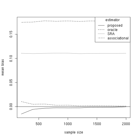
(a) T=2

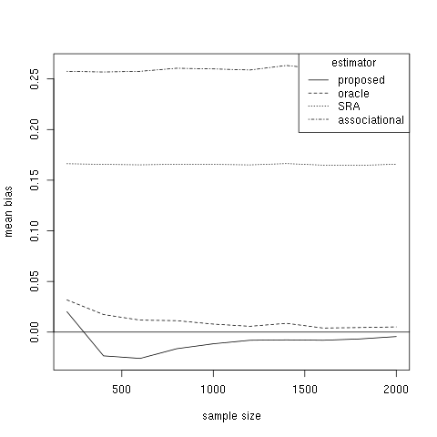
(b) T=3

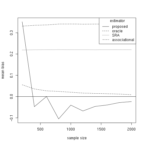
(c) T=4

Figure 5: Mean bias versus sample size of the proposed weighted estimator, for T=2, 3, and 4, time points, compared with oracle (weights including observed and unobserved confounders), SRA (weights including observed confounders), and associational (no weighting) estimators.

	T	n	bias	$\sigma_{mc}$	$\sigma_{sw}$	$\sigma_{bs}$	coverage (sw)	coverage (bs)
1	2	1000	0.03	1.40	1.55	7.96	0.99	0.99
2	2	2000	-0.06	0.72	0.71	1.31	0.99	0.99
3	2	3000	0.10	0.57	0.54	0.59	0.95	0.96
4	2	4000	0.02	0.44	0.46	0.48	0.96	0.96
5	2	5000	0.04	0.40	0.41	0.43	0.95	0.96
6	3	10000	-0.02	1.79	1.74	12.59	0.98	0.99
7	3	20000	0.09	0.95	0.97	1.33	0.96	0.99
8	3	30000	-0.02	0.75	0.75	0.81	0.96	0.97
9	3	40000	0.01	0.63	0.64	0.67	0.95	0.97
10	3	50000	-0.00	0.56	0.57	0.59	0.95	0.95
11	4	100000	-0.05	1.79	1.88	12.03	0.98	0.99
12	4	200000	-0.16	1.10	1.11	1.24	0.96	0.99
13	4	300000	0.17	0.92	0.92	0.97	0.97	0.97
14	4	400000	-0.01	0.79	0.80	0.83	0.95	0.95
15	4	500000	0.03	0.72	0.70	0.71	0.94	0.95

Table 2: Empirical bias, Monte Carlo $\sigma_{mc}$, sandwich $\sigma_{sw}$, and bootstrap $\sigma_{bs}$ standard deviations, and the coverage of nominal 95% sandwich and bootstrap CIs. The sandwich variance estimator appears more efficient than the bootstrap for this model, in contrast with the markov model discussed in Appendix 15. The jumps in sample size, approximately exponential in time $T$, are consistent with the discussion in Example 10 and Appendix 15. For our application, $T=2$ and $n\approx 270,000$.

The code used to carry out the simulations described above is available at https://github.com/haben-michael/iv-msmm. Also provided is an R package to estimate the parameters of an MSMM under the models described in Section 16.1 and Example 10.

7 Application

We examine the effect on neonatal mortality of delivery at a high-volume, high-technology hospital. High-level neonatal intensive care units (“NICUs”) have facilities for advanced care and average 50 or more premature births per year. Unadjusted analyses show a harmful association of delivery at a high-level NICU on neonatal mortality, but the effect is likely confounded. For example, more complicated pregnancies are often directed to high-level NICUs. Analyses controlling for a number of observed covariates have found a protective effect of delivery at a high-level NICU. Possible unmeasured confounders that remain in such analyses include unrecorded comorbidities on which a treating physician bases the decision to direct a mother to a high-level NICU. To account for these unmeasured confounders, Lorch et al. (2012) conducted an IV analysis using the relative distance of a mother’s residence to a high-level versus low-level NICU. This analysis found a protective effect. We consider the cumulative effect over time of delivery at a high-level NICU.

We consider a repeated measurements model $Y_{t}\sim\beta_{0}+\beta_{1}\sum_{\tau=1}^{t}A_{\tau}$, i.e.,

$$Y_{1} \sim\beta_{0}+\beta_{1}A_{1}$$

$$Y_{2} \sim\beta_{0}+\beta_{1}(A_{1}+A_{2}).$$

The outcome $Y_{t}$ represents the occurrence of an event at time $t$ and $A_{t}$ represents the treatment at time $t$, delivery at a high-level NICU, $t=1,2$. The parameters $(\beta_{0},\beta_{1})$ are the targets of inference, with $\beta_{1}$ representing the additive effect of cumulative treatment on neonatal mortality.

The data consists of 270,831 mothers who had exactly two births in Pennsylvania between 1995 and 2005. This data was drawn from a larger set consisting of all births in Pennsylvania between 1995 and 2005 for which birth certificates, death certificates and hospital records could be linked Lorch et al. (2012). The NICU level of the delivery hospital, coded based on previous work in four levels from least to most advanced facility, was dichotomized as “low” (levels 1, 2) and “high” (levels 3, 4). Delivery at a high-level NICU serves as the treatment $A_{t}$, for $t=1$ or $2$ representing the birth order. Our instrument $Z_{t}$ is the mother’s residence’s distance to the nearest low-level NICU minus nearest high-level NICU, dichotomized at $0$. That is, $Z_{t}>0$ indicates that a high-level NICU is closer than a low-level NICU to the mother’s residence. This IV is longitudinal in nature, with over 30% of the mothers changing residence between pregnancies, and about 10% of these changes in residence constituting a change in IV status.

Assumption 3 is supported by previous research suggesting that mothers tend to deliver at NICUs near their residence. In the data, the correlation between IV and treatment exceeds 60%. Assumption 7 requires that no population stratum consists deterministically of individuals living closer to a high-level NICU, nor does any stratum consist deterministically of individuals farther from a high-level NICU, where the population strata are determined by available covariates and the treatment and IV history. For example, regressing the IV at $T=2$ on available covariates and history, one finds a pseudo-$R^{2}$ of just 65.1%.

The remaining assumptions involve unobservables and cannot be directly tested using the data. Assumption 5 requires that the relative distance to a high-level or low-level NICU not affect neonatal outcomes except through the type of hospital at which the delivery occurred, conditional on available data. Assumption 6 requires that the mother’s relative distance to a high-level NICU is independent of unmeasured confounders of the association between NICU and neonatal death, at least upon controlling for socioeconomic data and other measured covariates. For example, the assumption requires that the relative distance of the mother’s residence is independent of the presence of unrecorded fetal heart tracing results, if these results indeed confound the relationship. Further discussion of the plausibility of the IV assumptions may be found in Lorch et al. (2012), which discusses a related IV, and qualifications may be found in Yang et al. (2014).

Assumption 8 requires that all factors are recorded that relate to whether a mother delivers at a high-level NICU when living closer to one. For example, if premature births are likely to occur at a high-level NICU irrespective of the mother’s residence’s distance, then the data ought to capture whether a birth is premature or not. Possible violations of this assumption are discussed in Yang et al. (2014).

The parameters $(\beta_{0},\beta_{1})$ were estimated as the solution to the estimating equation

$$\mathbb{P}_{n}\left(\begin{pmatrix}1&A_{1}\\ 1&A_{1}+A_{2}\end{pmatrix}^{T}\begin{pmatrix}W_{1}&0\\ 0&\overline{W}_{2}\end{pmatrix}\left(\begin{pmatrix}Y_{1}\\ Y_{2}\end{pmatrix}-\begin{pmatrix}1&A_{1}\\ 1&A_{1}+A_{2}\end{pmatrix}\begin{pmatrix}\beta_{0}\\ \beta_{1}\end{pmatrix}\right)\right).$$

The model for the density of the instrument conditional on the past observed history was modeled using a logistic regression. Likewise, $\Delta_{t}=\mathbb{P}(A_{t}=1\mid Z_{t}=1,\overline{L}_{t},\overline{A}_{t-1})-\mathbb{P}(A_{t}=1\mid Z_{t}=0,\overline{L}_{t},\overline{A}_{t-1})$ was estimated by first fitting $\mathbb{P}(A_{t}=1\mid Z_{t},\overline{L}_{t},\overline{A}_{t-1})$, again using a logistic regression. In both regressions, the covariates used were gestational age, mother’s educational level, and month that prenatal care began, following Yang et al. (2014). Besides this IV adjusted estimator, also computed were estimates using no weights, i.e., an associational estimate, and using SRA weights, using the covariates just described to form propensity scores.

The point estimates for $\beta_{1}$, given as the number of deaths per $10,000$ births, are 2.63 (associational), 2.91 (SRA), 1.46 (IV). This parameter represents the linear effect on neonatal mortality of the second of a mother’s first two deliveries at a high-level NICU. Bootstrap 95% CIs are $(1.54,3.56)$ (associational), $(2.06,4.10)$ (SRA), and $(-1.63,4.89)$ (IV). Thus while the associational and SRA analyses find a significantly harmful effect on neonatal mortality of delivery at a high-level NICU, the IV analysis fails to reject the null of no effect. The direction of these results is similar to the results reported in Lorch et al. (2012), though not as strong. There, unadjusted/associational analyses found a significantly harmful effect of delivery at a high-level NICU on infant death and other complications whereas the IV analysis found a significantly protective effect. Moreover, further IV analysis reported in Yang et al. (2014) finds little effect for most infants, similar to the result found here, with the significantly protective effect limited primarily to premature infants.

8 Discussion

We have shown how IVs may be used to identify causal parameters in marginal structural mean models. Most of our assumptions are mainly variations of standard IV or MSM assumptions. Our key assumption requires that unknown confounders not interact with the IV in the latter’s additive effect on the treatment. We further showed that the conclusion of our identification theorem requires an assumption of a similar form.

Several extensions to these results suggest themselves. First, the method of proof of our identification result may be generalized to apply to other MSMs besides mean models. In Cui et al. (2020), a Cox MSM for right-censored survival data is considered. The technical report Tchetgen Tchetgen et al. (2018) provides a theoretical framework for MSMs in general, although it lacks analysis of the finite-sample behavior and certain theoretical results for MSMMs given in the current work, such as the extension to continuous treatments.

Second, we have required that the instrumental variable be binary. Continuous IVs are often encountered, such as the difference in distances encountered in our application. Dichotomizing such IVs to fit our framework entails a loss of efficiency and may introduce other difficulties into the estimation procedure. Therefore, it would be useful to extend our identification and estimation results to allow for ordinal or continuous IVs. The resulting estimator would generalized two-stage least squares to the longitudinal setting in the way that the estimator proposed here generalizes the Wald estimator (Example 9).

Third, the estimator proposed here, the solution to the estimating equation (17), while convenient, does not make efficient use of all the available data. We expect improved performance from a robust, semiparametric efficient estimator.

9 Appendix: Markov model estimation

The data and model are described in Example 15. The treatment model given in (36),

$$\mathbb{P}(A_{t}=a \mid L_{t}=l,U_{t}=u,Z_{t}=z)=$$

$$(1-q)p_{L}^{\{l=a\}}(1-p_{L})^{\{l\neq a\}}+qp_{U}^{\{u=a\}}(1-p_{U})^{\{u\neq a\}}+(-1)^{1-z}(-1)^{1-a}\delta_{l}/2,$$

implies the observed-data model

$$\mathbb{P}(A_{t}=a\mid L_{t}=l,Z_{t}=z)=q/2+(1-q)p_{L}^{\{l=a\}}(1-p_{L})^{\{l\neq a\}}.$$

In order to identify the model we assume the mixing probability $q$ is known. For all $t$, the differences $\Delta_{t}$ are parametrized by $(\delta_{0},\delta_{1})$, and the remaining parameter for the treatment model is $p_{L}$. The MSMM model is

$$\mathbb{E}(Y_{\overline{a}})=m_{\beta}(\overline{a})=\beta\sum_{t}a_{t}.$$

As discussed in Section 16.1, outcomes consistent with this MSMM may be generated as

$$Y =\eta+\epsilon$$

$$\eta =\sum_{t=1}^{T}\tau_{t}(L_{t}-(1-q)p_{L}^{A_{t-1}}(1-p_{L})^{1-A_{t-1}}-q/2)+$$

$$\sum_{t=1}^{T}\rho_{t}(U_{t}-qp_{U}^{A_{t-1}}(1-p_{U})^{1-A_{t-1}}-(1-q)/2)+\mathbb{E}(Y_{\overline{a}}),$$

where $\epsilon$ is standard normal and exogenous, and $\tau_{t}=\rho_{t}=1,t=1,\ldots,T.$

Using the notation in Section 5, the parameters are the MSMM parameter $\beta,\alpha=(\delta_{0},\delta_{1})$ and $\nu=p_{L}$. Theorem 1 is used to estimate $\beta$ and $\alpha$ and $\nu$ are estimated by maximum likelihood. That is, the weighted residuals $\mathbb{P}_{n}(\sum_{t}A_{t})(Y-m_{\beta}(\overline{A}))/\overline{W}$ serve as an estimating equation for $\beta$ and the scores as estimating equations for $\alpha$ and $\nu$. Formulas for these scores and the information for all the parameters are obtained as in Section 16.2 by substituting

$$\pi_{\alpha,\nu}(A,L,Z) =q/2+(1-q)p_{L}^{L}(1-p_{L})^{1-L}$$

$$\frac{\partial\pi_{\alpha,\nu}}{\partial\alpha,\nu}(A,L,Z) =((-1)^{1-Z}(1-L)(\delta_{1}/\delta_{0})^{L},(-1)^{1-Z}(\delta_{0}/\delta_{1})^{1-L},$$

$$(1-q)L(1/p_{L}-1)^{1-L}-(1-q)(1-L)(1/p_{L}-1)^{-L}).$$

The second derivative $\frac{\partial^{2}\pi_{\alpha,\nu}}{\partial(\alpha,\nu)^{2}}$ is 0.

The results of a simulation are given in Table 4. In contrast to the model described in Section 6, the sandwich-derived CI appears more conservative than the bootstrap CI.

	T	n	bias	$\sigma_{mc}$	$\sigma_{sw}$	$\sigma_{bs}$	coverage (sw)	coverage (bs)
1	2	1000	0.02	26.92	21.34	28.33	0.99	0.97
2	2	2000	0.02	6.77	0.82	6.72	0.98	0.97
3	2	3000	-0.02	0.64	0.63	1.22	0.98	0.97
4	2	4000	0.02	0.55	0.53	0.88	0.97	0.96
5	2	5000	-0.02	0.45	0.46	0.60	0.98	0.97
6	3	10000	0.07	11.43	1.51	10.46	0.99	0.96
7	3	20000	-0.03	0.70	0.67	2.37	0.98	0.98
8	3	30000	-0.02	0.59	0.52	1.07	0.98	0.97
9	3	40000	0.04	0.47	0.42	0.50	0.96	0.96
10	3	50000	0.01	0.39	0.38	0.41	0.96	0.95
11	4	100000	0.01	4.57	1.56	8.51	0.98	0.97
12	4	200000	0.02	0.55	0.54	2.20	0.97	0.95
13	4	300000	-0.01	0.44	0.42	0.55	0.96	0.96
14	4	400000	0.01	0.39	0.35	0.38	0.95	0.95
15	4	500000	0.01	0.31	0.31	0.33	0.98	0.96

Table 4: Empirical bias, Monte Carlo standard deviation, sandwich sd, bootstrap sd, and the coverage of nominal 95% sandwich and bootstrap CIs, using the simple markov model discussed in Appendix 15.

10 Appendix: Continuous treatment density

We first show that the treatment density given in Example 4 is a valid density. As there, let the baseline density $f_{A_{t}\mid\operatorname{an}(A_{t})}(A_{t}=a,L_{t}=(l_{1},l_{2}),U_{t}=u,Z_{t}=0)$ be normal $\phi((a-l_{1})/u)/u$. The first component of the observed confounder $L_{t}$ controls the location and the unobserved confounder $U_{t}$ controls the spread. Let $\Delta_{t}(a\mid L_{t}=(l_{1},l_{2}))$ be a difference between normal densities that does not depend on $U_{t}$, say, $\phi(a)-\phi(a/l_{2})/l_{2}$. If the spread $u$ of the baseline density lies within an appropriate range, then $f_{A_{t}\mid\operatorname{an}(A_{t})}(A_{t}=a,L_{t}=(l_{1},l_{2}),U_{t}=u,Z_{t}=0)+\Delta_{t}(a)$ is a valid density for $A_{t}$. In particular, given $L_{t}=(l_{1},l_{2})$ with $l_{2}\in(0,1)$, suppose $l_{2}<u<\min(1,l_{2}/(1-l)2))$ for the standard deviation $u$ of the baseline. Let $l_{1}=0$ since the location is irrelevant to the argument. Then,

$$f_{A_{t}\mid\operatorname{an}(A_{t})}(A_{t}=a,L_{t}=(l_{1},l_{2}),U_{t}=u,Z_{t}=1)$$

$$=f_{A_{t}\mid\operatorname{an}(A_{t})}(A_{t}=a,L_{t}=(l_{1},l_{2}),U_{t}=u,Z_{t}=0)+\Delta_{t}(a)$$

$$=\phi(a/u)/u+\phi(a)-\phi(a/l_{2})/l_{2}$$

$$=\phi(a)\left\{1+\exp(a^{2}(1-1/u^{2})/2)/u-\exp(a^{2}(1-1/l_{2}^{2})/2)/l_{2}\right\}$$

$$=\phi(a)\exp(a^{2}(1-1/l_{2}^{2})/2)/l_{2}\left\{l_{2}\exp(a^{2}(1/l_{2}^{2}-1)/2)+(l_{2}/u)\exp(a^{2}(1/l_{2}^{2}-1/u^{2})/2)-1\right\}$$

$$\geq\phi(a)\exp(a^{2}(1-1/l_{2}^{2})/2)/l_{2}\left\{l_{2}+l_{2}/u-1\right\}$$

$$>0.$$

The first inequality follows from the condition that $l_{2}\in(0,1)$ and $l_{2}<u$, and the second inequality from the requirement $u<l_{2}/(1-l_{2})$. Since $\Delta_{t}$ integrates to 0 by construction, $f_{A_{t}\mid\operatorname{an}(A_{t})}(A_{t}=a,L_{t}=(l_{1},l_{2}),U_{t}=u,Z_{t}=1)$ is a valid density.

A small simulation using a continuous treatment density for a single time point is presented below. Following Example 4, $L$ and $U$ are sampled from a uniform distribution on the unit interval, $Z$ is a standard bernoulli, and the treatment density is defined as

$$\Delta(a\mid L) =\phi(a)-\phi(a/l)/l$$

$$f_{A\mid Z,L,U}(A=a,L=l,U=u) =\phi(a/u)/u+Z\Delta(a\mid L=l),$$

using $\phi$ to denote the standard normal density. The outcome is sampled as $Y=(L-\mathbb{E}(L))+(U-\mathbb{E}(U))+\beta A+\epsilon$, with $\beta=2$. The sample size is 1000. The observed bias and standard deviation of the estimates are -.195 and 0.64, and the median absolute error is .249. Figure 6 gives a histogram of the observed biases, as well as histograms of the weights and the plot of the conditional treatment density $f_{A\mid Z=1,L,U}$ for one choice of $L,U$.

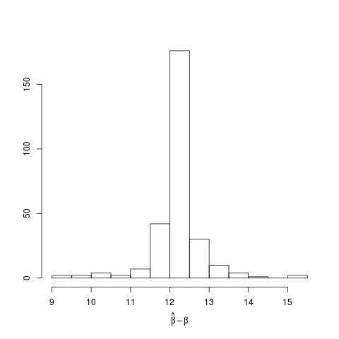
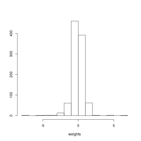
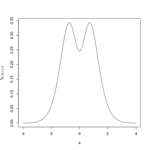
Figure 6: (Continuous treatment density.) The left panel is a histogram of the observed bias of the estimated coefficient in a simulation of size 1000. The middle panel is a histogram of the weights in one simulated data set. The right panel is a plot of the density $f_{A\mid Z=1,L,U}$, i.e., the sum of the baseline treatment density, which is normal, and the function $\Delta(a,l,u)$ for sample values of $l$ and $u$.

11 Appendix: Proof of Theorem 1

Proof.

To simplify notation, we use a single overbar and single time index to indicate a history of random vectors, e.g., $\overline{AZL}_{t}=(\overline{A}_{t},\overline{Z}_{t},\overline{L}_{t})=(A_{\tau},Z_{\tau},L_{\tau})_{\tau=0}^{\tau=t}$.

$$\mathbb{E}(\overline{W}^{-1}g(Y,\overline{A})) =\mathbb{E}(\overline{W}^{-1}\mathbb{E}(g(Y,\overline{A})\mid\overline{AZLU}))$$

$$=\int_{\mathcal{A}^{T}\times\mathcal{Z}^{T}\times\mathcal{L}^{T}\times\mathcal{U}^{T}}\overline{W}^{-1}\mathbb{E}(g(Y_{\overline{a}},\overline{a})\mid\overline{azlu})f_{\overline{AZLU}}(\overline{azlu})\mu_{\overline{AZLU}}(\overline{azlu})$$

The measure $\mu_{\overline{AZLU}}(\overline{azlu})$ is a product measure on $\mathcal{A}^{T}\times\mathcal{Z}^{T}\times\mathcal{L}^{T}\times\mathcal{U}^{T}$ relative to which the density $f_{\overline{AZLU}}$ is given, and analogously for $\mu_{\overline{A},\overline{Z}_{T-1}\overline{LU}}(\overline{a}\overline{z}_{T-1}\overline{lu})$ on $\mathcal{A}^{T}\times\mathcal{Z}^{T-1}\times\mathcal{L}^{T}\times\mathcal{U}^{T}$ and $f_{\overline{A}\overline{Z}_{T-1}\overline{LU}}$, and so forth. We have assumed the marginal measure $\mu_{Z_{t}},1\leq t\leq T,$ is counting measure on $\mathcal{Z}_{t}=\{0,1\}$.

Proceeding by induction, suppose we have established for some $s$, $0\leq s<T$,

$$\mathbb{E}(\overline{W}^{-1} g(Y,\overline{A}))=$$ (26)

$$\int_{\mathcal{A}^{T}\times\mathcal{Z}^{T-s}\times\mathcal{L}^{T-s}\times\mathcal{U}^{T-s}}\overline{W}^{-1}_{T-s}\mathbb{E}(g(Y_{\overline{a}},\overline{a})\mid\overline{azlu}_{T-s})f_{\overline{AZLU}_{T-s}}(\overline{azlu}_{T-s})\mu_{\overline{A},\overline{ZLU}_{T-s}}(\overline{a},\overline{zlu}_{T-s}).$$ (27)

By Assumption 5, (27) is

$$\mathbb{E}(\overline{W}^{-1}g(Y,\overline{A}))=\int_{\mathcal{A}^{T}\times\mathcal{Z}^{T-s}\times\mathcal{L}^{T-s}\times\mathcal{U}^{T-s}}\overline{W}^{-1}_{T-s}\mathbb{E}(g(Y_{\overline{a}},\overline{a})\mid\overline{a}_{T-s},\overline{z}_{T-s-1},\overline{lu}_{T-s})\times$$

$$f_{\overline{AZLU}_{T-s}}(\overline{azlu}_{T-s})\mu_{\overline{A},\overline{ZLU}_{T-s}}(\overline{a},\overline{zlu}_{T-s}).$$

By Assumption 6,

$$f_{\overline{AZLU}_{T-s}} =f_{A_{T-s}\mid\overline{A}_{T-s-1}\overline{ZLU}_{T-s}}\times f_{Z_{T-s}\mid\overline{AZ}_{T-s-1}\overline{LU}_{T-s}}\times f_{\overline{AZ}_{T-s-1}\overline{LU}_{T-s}}$$

$$=f_{A_{T-s}\mid\overline{A}_{T-s-1}\overline{ZLU}_{T-s}}\times f_{Z_{T-s}\mid\overline{AZ}_{T-s-1}\overline{L}_{T-s}}\times f_{\overline{AZ}_{T-s-1}\overline{LU}_{T-s}},$$

so (27) is the same as

$$\int_{\mathcal{A}^{T}\times\mathcal{Z}^{T-s}\times\mathcal{L}^{T-s}\times\mathcal{U}^{T-s}}\overline{W}^{-1}_{T-s-1}\mathbb{E}(g(Y_{\overline{a}},\overline{a})\mid\overline{a}_{T-s},\overline{z}_{T-s-1},\overline{lu}_{T-s})(-1)^{1-Z_{T-s}}\Delta_{T_{s}}^{-1}\times$$

$$f_{A_{T-s}\mid\overline{A}_{T-s-1}\overline{ZLU}_{T-s}}(\overline{azlu}_{T-s})f_{\overline{AZ}_{T-s-1}\overline{LU}_{T-s}}(\overline{az}_{T-s-1}\overline{lu}_{T-s})\mu_{\overline{A},\overline{ZLU}_{T-s}}(\overline{a},\overline{zlu}_{T-s})$$

$$=\int_{\mathcal{A}^{T}\times\mathcal{Z}^{T-s-1}\times\mathcal{L}^{T-s}\times\mathcal{U}^{T-s}}\overline{W}^{-1}_{T-s-1}\mathbb{E}(g(Y_{\overline{a}},\overline{a})\mid\overline{a}_{T-s},\overline{z}_{T-s-1},\overline{lu}_{T-s})\Delta_{T_{s}}^{-1}\times$$

$$\sum_{z\in\{0,1\}}(-1)^{z}f_{A_{T-s}\mid\overline{A}_{T-s-1}\overline{ZLU}_{T-s}}(\overline{alu}_{T-s},\overline{z}_{T-s-1},z_{T-s}=z)\times$$

$$f_{\overline{AZ}_{T-s-1}\overline{LU}_{T-s}}(\overline{az}_{T-s-1}\overline{lu}_{T-s})\mu_{\overline{A},\overline{Z}_{T-s-1},\overline{LU}_{T-s}}(\overline{a},\overline{z}_{T-s-1}\overline{lu}_{T-s})$$

$$=\int_{\mathcal{A}^{T}\times\mathcal{Z}^{T-s-1}\times\mathcal{L}^{T-s}\times\mathcal{U}^{T-s}}\overline{W}^{-1}_{T-s-1}\mathbb{E}(g(Y_{\overline{a}},\overline{a})\mid\overline{a}_{T-s},\overline{z}_{T-s-1},\overline{lu}_{T-s})\times$$

$$f_{\overline{AZ}_{T-s-1}\overline{LU}_{T-s}}(\overline{az}_{T-s-1}\overline{lu}_{T-s})\mu_{\overline{A},\overline{Z}_{T-s-1},\overline{LU}_{T-s}}(\overline{a},\overline{z}_{T-s-1}\overline{lu}_{T-s}).$$

Assumption 8 was used to cancel $\Delta_{T_{s}}^{-1}$ in obtaining the last equality. Applying Assumption 2 and integrating out $L_{t-s},U_{T-s}$, the last expression is

$$\int_{\mathcal{A}^{T}\times\mathcal{Z}^{T-s-1}\times\mathcal{L}^{T-s}\times\mathcal{U}^{T-s}}\overline{W}^{-1}_{T-s-1}\mathbb{E}(g(Y_{\overline{a}},\overline{a})\mid\overline{az}_{T-s-1},\overline{lu}_{T-s})\times$$

$$f_{\overline{AZ}_{T-s-1}\overline{LU}_{T-s}}(\overline{az}_{T-s-1}\overline{lu}_{T-s})\mu_{\overline{A},\overline{Z}_{T-s-1},\overline{LU}_{T-s}}(\overline{a},\overline{z}_{T-s-1}\overline{lu}_{T-s})$$

$$=\int_{\mathcal{A}^{T}\times\mathcal{Z}^{T-s-1}\times\mathcal{L}^{T-s-1}\times\mathcal{U}^{T-s-1}}\overline{W}^{-1}_{T-s-1}\mathbb{E}(g(Y_{\overline{a}},\overline{a})\mid\overline{azlu}_{T-s-1})\times$$

$$f_{\overline{AZLU}_{T-s-1}}(\overline{azlu}_{T-s-1})\mu_{\overline{A},\overline{ZLU}_{T-s-1}}(\overline{a},\overline{zlu}_{T-s-1}),$$

completing the inductive step. ∎

12 Appendix: Proof of Lemma 5

Proof.

The RHS of (11) does not depend on $z_{T}$ or $a^{\prime}_{T-1}$, so that $\mathbb{E}(Y_{\overline{a}}\mid\overline{a}_{T-1},a_{T}^{\prime},\overline{ZLU})=\mathbb{E}(Y_{\overline{a}}\mid\overline{a}_{T-1},a_{T}^{\prime},\overline{Z}_{T-1}\overline{LU})=\mathbb{E}(Y_{\overline{a}}\mid\overline{a}_{T-1},\overline{Z}_{T-1}\overline{LU}).$ Therefore,

$$\mathbb{E}(Y_{\overline{a}}\mid\overline{aZLU}_{T-1}) =\mathbb{E}(\mathbb{E}(Y_{\overline{a}}\mid\overline{aZ}_{T-1},\overline{LU})\mid\overline{aZLU}_{T-1})$$

$$=\mathbb{E}\left(m(\overline{a})+\sum_{t=1}^{T}\eta_{t}(\overline{a},\overline{aZ}_{t-1},\overline{LU}_{t})\biggm{|}\overline{aZLU}_{T-1}\right)$$

$$=m(\overline{a})+\sum_{t=1}^{T-1}\eta_{t}(\overline{a},\overline{aZ}_{t-1},\overline{LU}_{t}),$$

and by induction, $\mathbb{E}(Y_{\overline{a}}\mid\overline{azlu}_{t})=m(\overline{a})+\sum_{t^{\prime}=1}^{t}\eta_{t^{\prime}}(\overline{a},\overline{az}_{t^{\prime}-1},\overline{lu}_{t^{\prime}})$ for all $t$. Consequently, $\mathbb{E}(Y_{\overline{a}}\mid\overline{a}_{t-1},a_{t}^{\prime},\overline{ZLU})=\mathbb{E}(Y_{\overline{a}}\mid\overline{a}_{t-1},a_{t}^{\prime},\overline{Z}_{t-1}\overline{LU})=\mathbb{E}(Y_{\overline{a}}\mid\overline{a}_{t-1},\overline{Z}_{t-1}\overline{LU})$ for all $t$, so that the data satisfy Assumption 2^′ and 5. Additionally, $\mathbb{E}(Y_{\overline{a}})=\mathbb{E}(\mathbb{E}(Y_{\overline{a}}\mid L_{1}U_{1}))=\mathbb{E}(m(\overline{a})+\eta_{1}(\overline{a},\overline{LU}_{1}))=m(\overline{a}),$ so the data satisfies the MSMM given by $m(\overline{a})$. Finally, $Y$ is defined in (12) so as to satisfy Assumption 1^′. Therefore, so long as $\eta$ satisfies (11), outcomes $Y$ satisfying (12) are consistent with the assumptions implying the identification result (10). ∎

13 Appendix: Proof of Theorem 6

Proof.

In view of Lemma 5, (13) is equivalent to the requirement that

$$\mathbb{E}(h(\overline{A_{T}})\omega_{T}(ALZ_{T})\eta(\overline{AZLU}_{T}))=0$$

hold for any choice of $T,h$ and $\eta$ as in (11). An example of such $\eta$ is any function of $\overline{AZ}_{T-1}\overline{LU}_{T}$ conditionally mean-zero given $\overline{AZLU}_{t-1}$, i.e., $\zeta(\overline{AZ}_{T-1}\overline{LU}_{T})-\mathbb{E}(\zeta(\overline{AZ}_{T-1}\overline{LU}_{T})\mid\overline{AZLU}_{T-1})$ for arbitrary $\zeta\in L_{1}(\overline{AZ}_{T-1}\overline{LU}_{T})$. The condition becomes

$$\mathbb{E}(h(\overline{A}_{T})\omega_{T}(\overline{ALZ}_{T})\zeta(\overline{AZ}_{T-1}\overline{LU}_{T})) =\mathbb{E}(h(\overline{A}_{T})\omega_{T}(\overline{ALZ}_{T})\mathbb{E}(\zeta(\overline{AZ}_{T-1}\overline{LU}_{T})\mid\overline{AZLU}_{T-1}))$$

$$=\mathbb{E}(\mathbb{E}(h(\overline{A}_{T})\omega_{T}(\overline{ALZ}_{T})\mid\overline{AZLU}_{T-1})\zeta(\overline{AZ}_{T-1}\overline{LU}_{T})),$$

for all $\zeta\in L_{1}(\overline{AZ}_{T-1}\overline{LU}_{T})$, implying that $\mathbb{E}(h(\overline{A}_{T})\omega_{T}(\overline{ALZ}_{t})\mid\overline{AZLU}_{T-1})$ is a version of the conditional expectation $\mathbb{E}(h(\overline{A}_{T})\omega_{T}(\overline{ALZ}_{T})\mid\overline{AZ}_{T-1}\overline{LU}_{T})$, i.e., $h(\overline{A}_{T})\omega_{T}(\overline{ALZ}_{T})$ is conditionally mean-independent of $L_{T},U_{T}$ given $\overline{AZLU}_{T-1}$.

Taking $h(\overline{A}_{T})=\{\overline{A}_{T}=\overline{a}_{T}\}$ for $\overline{a}_{T}\in\mathcal{A}^{T}$,

$$\sum_{z_{T}\in\mathcal{Z}}f_{A_{T}\mid...}(a_{T}\mid\overline{A}_{T-1},\overline{Z}_{T-1},z_{T},\overline{LU}_{T})\omega_{T}(\overline{A}_{T-1},a_{T},\overline{Z}_{T-1},z_{T},\overline{L}_{T})f_{z_{T}\mid...}(z_{T}\mid\overline{AZ}_{T-1}\overline{L}_{T})$$

$$\sum_{z_{T}\in\mathcal{Z}}f_{A_{T}\mid...}(a_{T}\mid\overline{A}_{T-1},\overline{Z}_{T-1},z_{T},\overline{LU}_{T})\omega_{T}(\overline{A}_{T-1},a_{T},\overline{Z}_{T-1},z_{T},\overline{L}_{T})f_{z_{T}\mid...}(z_{T}\mid\overline{AZ}_{T-1}\overline{LU}_{T})$$

$$=\mathbb{E}(f_{A_{T}\mid...}(a_{T}\mid\overline{A}_{T-1}\overline{ZLU}_{T})\omega_{T}(\overline{A}_{T-1},a_{T},\overline{ZL}_{T})\mid\overline{AZ}_{T-1}\overline{LU}_{T})$$

$$=\mathbb{E}(\{A_{T}=a_{T}\}\omega_{T}(\overline{A}_{T-1},a_{T},\overline{ZL}_{T})\mid\overline{AZ}_{T-1}\overline{LU}_{T})$$

$$=\mathbb{E}(\{A_{T}=a_{T}\}\omega_{T}(\overline{A}_{T-1},a_{T},\overline{ZL}_{T})\mid\overline{AZLU}_{T-1})$$

In particular, $\sum_{z_{T}\in\mathcal{Z}}f_{A_{T}\mid...}(a_{T}\mid\overline{A}_{T-1},\overline{Z}_{T-1},z_{T},\overline{LU}_{T})\omega_{T}^{\prime}(\overline{A}_{T-1},a_{T},\overline{Z}_{T-1},z_{T},\overline{L}_{T})$ is mean-independent of $(L_{T},U_{T})$ given $\overline{aZLU}_{T-1}$, where

$$\omega_{T}^{\prime}(\overline{A}_{T-1},a_{T},\overline{Z}_{T-1},z_{T},\overline{L}_{T})=\omega_{T}(\overline{A}_{T-1},a_{T},\overline{Z}_{T-1},z_{T},\overline{L}_{T})f_{z_{T}\mid...}(z_{T}\mid\overline{AZ}_{T-1}\overline{L}_{T}).$$

Since $T$ was arbitrary, the result follows.

∎

14 Appendix: Linear omitted variables model, comparing biases

Given a linear MSMM, suppose an estimator is obtained as the root of weighted estimating equations

$$\mathbb{P}_{n}\left(\omega h(\overline{A})\left(Y-\beta^{T}\overline{A}\right)\right)=0$$

where the weight $\omega$ is an integrable function of the observed data $(\overline{A},\overline{Z},\overline{L})$. This root is a weighted least squares estimator

$$\hat{\beta}=\left(\mathbb{P}_{n}(\omega h(\overline{A})\overline{A}^{T})\right)^{-1}\mathbb{P}_{n}\left(\omega h(\overline{A})Y\right).$$ (28)

Suppose the data satisfy the assumptions of Theorem 1 and the observed outcome is

$$Y=\sum_{t}(\beta_{L_{t}}g_{L_{t}}(L_{t})+\beta_{U_{t}}g_{U_{t}}(U_{t}))+\beta^{T}\overline{A}+\epsilon,$$

with $\epsilon$ exogenous, $\beta_{L_{t}},\beta_{U_{t}}\in\mathbbm{R}^{p}$, and $\mathbb{E}(g_{L_{t}}(L_{t})\mid\overline{L}_{t-1},\overline{A}_{t-1})=\mathbb{E}(g_{U_{t}}(U_{t})\mid\overline{U}_{t-1},\overline{A}_{t-1})=0$. As discussed in the passage following Lemma 5, this outcome model is consistent with the MSMM

$$\mathbb{E}(Y_{\overline{a}})=\beta^{T}\overline{a}.$$

The estimator (28) is

$$\hat{\beta}=\left(\mathbb{P}_{n}\left(h(\overline{A})\overline{A}^{T}/\omega\right)\right)^{-1}\mathbb{P}_{n}\left(\omega^{-1}h(\overline{A})\left(\sum_{t}(\beta_{L_{t}}g_{L_{t}}(L_{t})+\beta_{U_{t}}g_{U_{t}}(U_{t})+\epsilon)\right)\right)+\beta.$$

We consider the asymptotic bias of this estimator,

$$\operatorname{plim}\hat{\beta}-\beta=\left(\mathbb{P}_{n}\left(h(\overline{A})\overline{A}^{T}/\omega\right)\right)^{-1}\mathbb{P}_{n}\left(\omega^{-1}h(\overline{A})\left(\sum_{t}(\beta_{L_{t}}g_{L_{t}}(L_{t})+\beta_{U_{t}}g_{U_{t}}(U_{t}))\right)\right),$$

for various choices of weights $\omega$.

When $\omega=1$, the resulting estimator $\hat{\beta}$, known as the “associational” or “crude” estimator, ignores all confounding. The implied model is misspecified by omitting covariates $L_{t},U_{t}$. The bias is

$$\left(\mathbb{E}\left(h(\overline{A})\overline{A}^{T}\right)\right)^{-1}\mathbb{E}\left(h(\overline{A})\left(\sum_{t}g_{L_{t}}(L_{t})+g_{U_{t}}(U_{t})\right)\right).$$

This bias is related to the strength of the dependency between the treatments and all confounders, known and unknown. When $g_{L_{t}}$, $g_{U_{t}}$, and $h$ are linear, for example, the bias is linear in the covariance between the treatments and the sum of the confounders.

The SRA estimator, given by the choice $\omega=1/\overline{W}^{(SRA)}=1/\prod_{t}f(A_{t}\mid\overline{L}_{t},\overline{A}_{t-1})$, has bias

$$\left(\mathbb{E}\left(h(\overline{A})\overline{A}^{T}/\prod_{t}f(A_{t}\mid L_{t},A_{t-1})\right)\right)^{-1}\mathbb{E}\left(\frac{h(\overline{A})\sum_{t}(\beta_{L_{t}}g_{L_{t}}(L_{t})+\beta_{U_{t}}g_{U_{t}}(U_{t}))}{\prod_{t}f(A_{t}\mid L_{t},A_{t-1})}\right).$$ (29)

Since it is assumed $\mathbb{E}(g_{L_{T}}(L_{T})\mid A_{T-1},L_{T-1})=0$,

$$\mathbb{E}\left(\frac{h(\overline{A})g_{L_{T}}(L_{T})}{\prod_{t=1}^{T}f(A_{t}\mid L_{t},A_{t-1})}\right) =\mathbb{E}\left(\mathbb{E}\left(\frac{h(\overline{A})g_{L_{T}}(L_{T})}{\prod_{t=1}^{T}f(A_{t}\mid L_{t},A_{t-1})}\biggm{|}L_{T},A_{T-1}\right)\right)$$

$$=\mathbb{E}\left(\int_{\mathcal{A}}\frac{h(\overline{A}_{T-1},a_{T})g_{L_{T}}(L_{T})}{\prod_{t=1}^{T-1}f(A_{t}\mid L_{t},A_{t-1})}\mu_{A_{T}}(a_{T})\right)$$

$$=\mathbb{E}\left(\int_{\mathcal{A}}\frac{h(\overline{A}_{T-1},a_{T})}{\prod_{t=1}^{T-1}f(A_{t}\mid L_{t},A_{t-1})}\mu_{A_{T}}(a_{T})\times\mathbb{E}\left(g_{L_{T}}(L_{T})\mid A_{T-1},L_{T-1}\right)\right)=0,$$

and similarly for $t<T$. The inverted factor in (29) is, by (5), $\int_{\mathcal{A}}h(\overline{a})\overline{a}^{t}\mu_{\overline{A}}(\overline{a})$. The resulting expression

$$\left(\int_{\mathcal{A}}h(\overline{a})\overline{a}^{t}\mu_{\overline{A}}(\overline{a})\right)^{-1}\mathbb{E}\left(h(\overline{A})\left(\sum_{t}g_{U_{t}}(U_{t})\right)/\overline{W}^{(SRA)}\right),$$

shows that the bias is a quantity related to the dependence between the treatment and unknown confounders, as expected due to the violation of SRA. In comparison with the bias of the associational estimator, the term corresponding to treatment and known confounder dependency is eliminated. As $\sum_{t}g_{U_{t}}(U_{t})$ and $h(\overline{A})/\overline{W}^{(SRA)}$ are generally correlated when $U_{t}$ are in fact confounders, the bias is nonzero.

When $\omega$ are the IV weights (8), the asymptotic bias is zero since we have assumed the conditions of Theorem 1, which entails

$$\mathbb{E}\left(\overline{W}^{-1}h(\overline{A})\sum_{t}\left(\beta_{L_{t}}g_{L_{t}}(L_{t})+\beta_{U_{t}}g_{U_{t}}(U_{t})\right)\right)=\mathbb{E}\left((\overline{W}^{-1}h(\overline{A})(Y-m_{\beta}(\overline{A}))\right)-\mathbb{E}\left(\overline{W}^{-1}h\cdot\epsilon\right)=0.$$

A Monte Carlo simulation comparing these three estimators is described in Section 6.

15 Appendix: Two-state markov chain

We examine the relationship between confounding and the variance of the estimator obtained from the estimating equation (17), using a simple model to compare expressions in the SRA and IV contexts.

SRA weights include probability densities at each time point, and IV weights include a difference of densities. As the number of time points $T$ grows and these weights are multiplied, an estimator may quickly become unstable. Let $\hat{\beta}$ be obtained as the solution to (17). Assuming standard regularity conditions, the asymptotic variance of $\hat{\beta}$ is the variance of the influence function,

$$\operatorname{Var}(\sqrt{n}(\hat{\beta}-\beta_{0}))\to\left(\mathbb{E}\frac{\partial}{\partial\beta}(hm_{\beta}/\overline{W})\right)^{-2}\mathbb{E}\left((h(\overline{A})(Y-m_{\beta})/\overline{W})^{2}\right).$$ (30)

In this display, the weights $\overline{W}$ refer generically to either SRA weights (7) or IV weights (8). The term $h(\overline{A})m_{\beta}(\overline{A})$ is a function of the treatments, so by (5), in the case $\overline{W}$ are SRA weights, or by Theorem 1, in the case of IV weights,

$$\mathbb{E}\frac{\partial}{\partial\beta}\left(hm_{\beta}/\overline{W}\right)|_{\beta=\beta_{0}}=\int\frac{\partial}{\partial\beta}hm_{\beta}d\mu_{\overline{A}}$$

does not depend on the weights. A first order approximation to the asymptotic variance is

$$\left(\int\frac{\partial}{\partial\beta}hm_{\beta}d\mu_{\overline{A}}\right)^{-2}\mathbb{E}\left((h(\overline{A})(Y-m_{\beta}))^{2}\right)\mathbb{E}\left(1/\Pi_{t}W_{t}^{2}\right).$$ (31)

This expression appears to grow exponentially in the number of time points. In the SRA framework, various techniques have been proposed to stabilize the weights. These involve using a function of the treatments to cancel out the weights, functions of both treatment and confounders. The stability of the weights therefore depends on the strength of the dependence between treatment and confounder, a relationship that can be quantified in simple models. We consider analogous stabilization for the IV estimator.

SRA weights. Suppose treatment and covariates are binary, and

$$\begin{aligned} \mathbb{P}(L_{t}\mid\operatorname{an}(L_{t}))&=\mathbb{P}(L_{t}\mid A_{t-1})=p_{LA},\\ \mathbb{P}(A_{t}\mid\operatorname{an}(A_{t}))&=\mathbb{P}(A_{t}\mid L_{t-1})=p_{AL},\\ \mathbb{P}(L_{1}=0)&=\mathbb{P}(L_{1}=1)=1/2.\end{aligned}$$ (32)

The data is a two-state markov chain with alternating doubly stochastic transition matrices,

$$\begin{pmatrix}p_{LA}&1-p_{LA}\\ 1-p_{LA}&p_{LA}\end{pmatrix},\begin{pmatrix}p_{AL}&1-p_{AL}\\ 1-p_{AL}&p_{AL}\end{pmatrix}.$$

Figure 7: DAG for the two-state markov model meeting the sequential randomization assumption, with 2 time points.

The parameter $p_{LA}$ is the probability that the state of $A_{t+1}$ is the same as $L_{t}$. It may be interpreted as the strength of the dependence of $A$ on $L$, a type of confounding, with the strongest confounding occurring as $p_{LA}$ nears the border of $[0,1]$, and the weakest at $p_{LA}=.5$. The situation is analogous for $p_{AL}$. The marginal distributions of both $L_{t}$ and $A_{t},t=1,\ldots,T,$ are bernoulli with success probability 1/2.

The SRA weights are $\prod_{t}f(A_{t}\mid L_{t-1})=\prod_{t}p_{LA}^{\{A_{t}=L_{t-1}\}}(1-p_{LA})^{\{A_{t}\neq L_{t-1}\}}=(1-p_{LA})^{T}\prod_{t}(p_{LA}/(1-p_{LA}))^{\{A_{t}=L_{t-1}\}}$. Because $\mathbb{E}(\{A_{t}=L_{t-1}\}\mid A_{t-1})=p_{LA}$ and the states are binary, the factors that make up the weights are independent and identically distributed, and

$$\mathbb{E}(1/\overline{W}^{2})=(\mathbb{E}(1/W_{1}^{2}))^{T}=(p_{LA}(1-p_{LA}))^{-T}.$$ (33)

The variance is polynomial in the inverse of $p_{LA}(1-p_{LA})$, a measure of treatment–covariate dependence, with order given by the number of time points $T$. The parameter $p_{AL}$ determining $A_{t-1}\to L_{t}$ transitions does not play a role, although it plays the main role in weight stabilization discussed below. The dependence on $p_{LA}$ is through $p_{LA}(1-p_{LA})=1/4-(p_{LA}-1/2)^{2}$, so that (33) is minimized over $p_{LA}$ at $1/2$, when treatment and covariate are independent, and increases without bound as $|p_{LA}-1/2|\to 1/2$.

Although the focus on this example is the behavior of the weights, an estimate of the variance of the full estimator is straightforward once an outcome model is specified. Suppose the observed outcome $Y$ satisfies

$$\mathbb{E}(Y\mid\overline{A},\overline{Z},\overline{L},\overline{U})=\lambda\sum_{t}(L_{t}-\mathbb{E}(L_{t}\mid\overline{L}_{t-1},\overline{A}_{t-1}))+\beta\sum_{t}A_{t}+\epsilon,$$

where $\epsilon$ has mean zero and variance $\sigma^{2}$. While parameter $p_{LA}$ describes one part of confounding, the dependence of treatment on the confounding covariate, the parameter $\lambda$ describes the other part of confounding, the dependence of the outcome on the covariate. By Lemma 5, this model for $Y$ is consistent with the MSMM

$$\mathbb{E}(Y_{\overline{a}})=\beta\sum_{t}a_{t}.$$

It follows that the first order approximation (31) is

$$\frac{\lambda^{2}(1+\sigma^{2}/(Tp_{LA}(1-p_{LA})))}{(T+1)(4p_{LA}(1-p_{LA}))^{T-1}}$$ (34)

The principal difference from the second moment of the weights (33) is that the exponent is $T-1$ rather than $T$, and quadratic dependence on $\lambda$. A plot of the dependence on $p_{LA}$, along with the empirical variance from a small simulation to indicate the quality of the approximation, is given in Fig. 8.

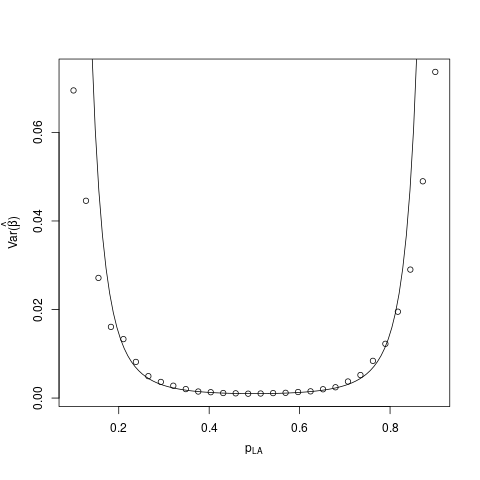
Figure 8: The variance of the unstabilized SRA estimator $\hat{\beta}$ in the two-state markov model. The solid line is the first-order approximation (34) and the plotted characters come from a Monte Carlo simulation. For the simulation the number of time points $T$ is $7$ and sample size is $500$.

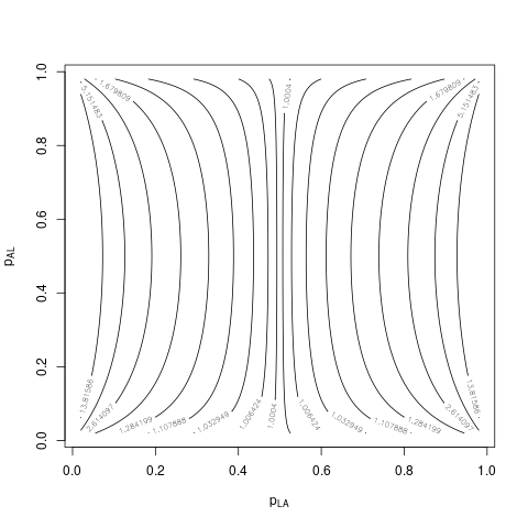
Figure 9: Variance of stabilized SRA weights in the two-state markov model. The variance blows up as $p_{LA}$ approaches 0 or 1, as in the unstabilized case, but remains bounded if $p_{AL}$ approaches 0 or 1 with at least the same rate.

Modified weights are often used to mitigate the instability of the SRA estimator. A factor $h^{\prime}$ in the function $h(\overline{A})$ is chosen to approximate $f(A_{t}|\overline{L}_{t},\overline{A}_{t-1})$, with a view to minimizing the mean square of the influence function (30). In the trivial case that $L$ is not in fact a confounder, $h^{\prime}$ may be taken to be $f(A_{t}|\overline{L}_{t},\overline{A}_{t-1})=f(A_{t}|\overline{A}_{t-1})$. The weights are cancelled out and the estimator is no longer exponential in $T$. In general, the quality of an approximation of $f(A|L)$ using a function of $A$ depends on how well $A$ predicts $L$, controlled in this example by $p_{AL}$. The variance of the influence function (30) does not change on multiplying $h$ by a constant, so the minimization is well-posed, and there is no loss of generality to assume $\int h^{\prime}=1$.

A common choice of stabilized weights, which we consider, uses the density $f(A_{t}|\overline{A}_{t-1})$ as the approximation to $f(A_{t}|\overline{L}_{t},\overline{A}_{t-1})$, that is, $h$ contains as a factor the joint density of $\overline{A}$. For the two-state markov model, the markov property gives as stabilized weights,

$$\overline{W}=\prod_{t}\frac{f(A_{t}|L_{t})}{f(A_{t}\mid A_{t-1})}.$$

The factors are again i.i.d., and the second moment of the inverted weights is computed to be

$$\mathbb{E}(1/\overline{W}^{2})=\left(\mathbb{E}(\frac{f(A_{2}\mid A_{1})}{f(A_{2}\mid L_{1})})\right)^{T}=\left(1+4\frac{p_{AL}(1-p_{AL})}{p_{LA}(1-p_{LA})}(p_{LA}-1/2)^{2}\right)^{T}.$$

Holding $T$ fixed, consider the behavior of the variance as the parameters $p_{LA},p_{AL}$ vary. When $p_{LA}=p_{AL}=p$, this expression is $(1+4(p-1/2))^{T}$, and the blowup at the boundary points present in the case of unstabilized weights is eliminated (Fig. 9). For $p\in[0,1]$ let $\rho(p)=p(1-p)=1/4-(p-1/2)^{2}$, a measure of the distance of $p$ to the boundary of $[0,1]$. With this notation,

$$\mathbb{E}(1/\overline{W}^{2})=\left(1+4\frac{\rho(p_{AL})}{\rho(p_{LA})}(p_{LA}-1/2)^{2}\right)^{T}\leq\left(1+\frac{\rho(p_{AL})}{\rho(p_{LA})}\right)^{T}.$$ (35)

The behavior of stabilized weights as $p_{LA}$ nears the boundary of $[0,1]$ is governed not by $1/\rho(p_{LA})$, as in the unstabilized case, but the ratio $\rho(p_{AL})/\rho(p_{LA})$, and will be bounded when $\rho(p_{AL})=\mathcal{O}(\rho(p_{LA}))$. Qualitatively, this situation occurs when the degree of treatment-covariate confounding does not grow faster than the treatment’s predictiveness of the covariate.

Next, let $T$ grow. It follows from (35) that the variance can be stabilized by controlling the decay of $\rho(p_{AL})/\rho(p_{LA})$. By comparison with $t\mapsto(1+1/t)^{t}$ it follows $\rho(p_{AL})/\rho(p_{LA})=\mathcal{O}(1/T)$ is sufficient. This possibility is not available with unstabilized weights. Since $p_{AL}(1-p_{AL})\leq 1/4$, the unstabilized weight moment (33) $(p_{AL}(1-p_{AL}))^{-T}\geq 4^{T}$ always diverges with $T$.

IV weights.

We next consider an extension of the two-state markov model (32) in order to examine the behavior of the IV weights in relation to confounding. The states $L_{t}$ are augmented with additional binary variables $U_{t}$ and $Z_{t}$, giving rise to a process $\ldots(L_{t-1},U_{t-1},Z_{t-1})\to A_{t-1}\to(L_{t},U_{t},Z_{t})\to A_{t}\ldots$ . For $q,p_{L},p_{U}\in(0,1)$ and suitable $\delta_{0},\delta_{1}$, as discussed below, define transition probilities through

$$\begin{aligned} \mathbb{P}(A_{t}=a\mid\operatorname{an}(A_{t}))&=\mathbb{P}(A_{t}=a\mid L_{t}=l,U_{t}=u,Z_{t}=z)\\ &=\mathbb{P}(A_{t}=a\mid L_{t}=l,U_{t}=u)+(-1)^{1-z}(-1)^{1-a}\delta_{l}/2\\ \mathbb{P}(A_{t}=a\mid L_{t}=l,U_{t}=u)&=(1-q)p_{L}^{\{l=a\}}(1-p_{L})^{\{l\neq a\}}+qp_{U}^{\{u=a\}}(1-p_{U})^{\{u\neq a\}}\\ \mathbb{P}(L_{t+1}=l,U_{t+1}=u,Z_{t+1}=z&\mid A_{t}=a,\operatorname{an}(L_{t+1},U_{t+1},Z_{t+1}))=\mathbb{P}(Z_{t+1}=z)\mathbb{P}(L_{t+1}=l,U_{t+1}=u\mid A_{t}=a)\\ &=(1/4)\mathbb{P}(A_{t}=a\mid L_{t}=l,U_{t}=u)\\ \mathbb{P}(Z_{t}=z)&=1/2.\end{aligned}$$ (36)

The initial state $(L_{1},U_{1},Z_{1})$ is distributed as three i.i.d. symmetric bernoulli variables. It follows that the marginal distribution of each of $L_{t},U_{t},A_{t},t=1,\ldots,$ is bernoulli with success probability 1/2, as with $Z_{t}$. A DAG is given in Fig. 10.

Figure 10: DAG for the two-state markov model with unknown confounding and IV, with 2 time points.[[links between L and U]]

Figure 11: The distribution of the two-state markov model with unknown confounding (36) may be obtained by combining two chains with no unknown confounders (See Fig. 7). Corresponding covariate states $L_{t}$ and $U_{t}$ are concthatenated along with an exogenous IV to give the new covariate state $(L_{t},U_{t},Z_{t})$. The new treatment states are obtained by mixing with probability $q$, $A_{t}\coloneqq B_{t}A_{t}^{L}+(1-B_{t})A_{t}^{U}$, with $B_{t}$ i.i.d. bernoulli with parameter $q$.

The model for the conditional density of $A_{t}$ given $(L_{t},U_{t},Z_{t})$ may be described by parameters $p_{lu}=\mathbb{P}(A=0\mid Z=0,L=l,U=u)\in[0,1]$ and $\delta_{l}$ for $l,u\in\{0,1\}$; see Table 5. Requiring $|\delta_{l}|<1/2-\max(|p_{l0}-1/2|,|p_{l1}-1/2|)$ ensures $\mathbb{P}(a_{t}\mid l_{t},u_{t},z_{z})>0$. Summing horizontally in Table 5 shows $\sum_{a}\mathbb{P}(a_{t}\mid l_{t},u_{t},z_{t})=1$. Therefore $\mathbb{P}(a_{t}\mid l_{t},u_{t},z_{t})$ is a valid density. Moreover, Assumption 8 is satisfied since

$$\Delta_{t}(\overline{a}_{t},\overline{z}_{t-1},\overline{l}_{t},\overline{u}_{t})\equiv \sum_{z_{t}\in\{0,1\}}(-1)^{1-z_{t}}\mathbb{P}(A_{t}=a_{t}\mid\overline{L}_{t}=\overline{l}_{t},\overline{U}_{t}=\overline{u}_{t},\overline{Z}_{t-1}=\overline{z}_{t-1},Z_{t}=z,\overline{A}_{t-1}=\overline{a}_{t-1})$$

$$=\sum_{z_{t}\in\{0,1\}}(-1)^{1-z_{t}}\mathbb{P}(A_{t}=a_{t}\mid L_{t}=l_{t},U_{t}=u_{t},Z_{t}=z_{t})$$

$$=(-1)^{1-a_{t}}\delta_{l_{t}}$$

does not depend on $\overline{u}_{t}$. The magnitude of $\delta_{0}$ and $\delta_{1}$ are interpretable as IV strength. Their difference $|\delta_{1}-\delta_{0}|$ gives the dependence of $\delta$ on $L_{t}$, which has an analogous role in weight stabilization to the treatment-confounder dependence $p_{LA}$ parameter in the SRA setting. That is, to the extent that this dependence may be approximated by a standardized function of $\overline{A}$, an analogue of stabilized weights may be used to decrease the variance of the estimator.

The parameters $q,p_{L},p_{U}$ used to describe the model (36) are not identified by the data $(A_{t},Z_{t},L_{t},U_{t})$, nor are the observed parameters $q,p_{L}$ identified by the observed data $(A_{t},Z_{t},L_{t})$. We use them because they allow for easy comparison with the SRA case. For purposes of estimation (e.g., Appendix 15), an identifying condition like $p_{B}=1/2$ or $p_{L}=p_{U}$ is needed, or reparameterization.

The distribution of the resulting markov chain can also be obtained by mixing two independent chains of the type described in the ((ref sra section above)), say, $\ldots\to L_{t-1}\to A_{t-1}^{L}\to L_{t}\to\ldots$ with parameters $p_{AL},p_{LA}$, and $\ldots\to U_{t-1}\to A_{t-1}^{U}\to U_{t}\to\ldots$ with parameters $p_{AU},p_{UA}$. See Fig. 11. Corresponding covariate states $L_{t}$ and $U_{t}$ are concatenated along with an exogenous IV to give the new covariate state $(L_{t},U_{t},Z_{t})$. The new treatment states are obtained by mixing with probability $q$, $A_{t}=B_{t}A_{t}^{L}+(1-B_{t})A_{t}^{U}$, with $B_{t}$ i.i.d. bernoulli with parameter $q$. The mixing parameter $q$ controls the relative dependence of the treatment on known confounding as compared with unknown confounding. The IVs are then added as independent, exogenous perturbations of the new treatment states $A_{t}$ in such a way that the Assumption 8 is satisfied. The parameters $p_{LA},p_{AL},p_{UA},$ and $p_{AU}$ have similar interpretations as before.

Table 5: The conditional treatment densities $\mathbb{P}(A=a\mid L=l,U=u,Z=z)$ for the two-state markov model with IVs. The densities are the same at all times. There are 6 parameters, $p_{lu}\in[0,1]$ and $\delta_{l}$ for $l,u\in\{0,1\}$. The magnitude of $\delta_{0}$ and $\delta_{1}$ are interpretable as IV strength. Their difference $|\delta_{1}-\delta_{0}|$ gives the dependence of $\delta$ on $L_{t}$, which has an analogous role in weight stabilization to the treatment-confounder dependence parameter $p_{LA}$ in the SRA setting.

$U=1$	$Z=1$	$p_{01}\pm\delta_{0}$	$\overline{p_{01}}\mp\delta_{0}$	$p_{11}\pm\delta_{1}$	$\overline{p_{11}}\mp\delta_{1}$
	$Z=0$	$p_{01}$	$\overline{p_{01}}$	$p_{11}$	$\overline{p_{11}}$
$U=0$	$Z=1$	$p_{00}\pm\delta_{0}$	$\overline{p_{00}}\mp\delta_{0}$	$p_{01}\pm\delta_{1}$	$\overline{p_{01}}\mp\delta_{1}$
	$Z=0$	$p_{00}$	$\overline{p_{00}}$	$p_{01}$	$\overline{p_{01}}$
		$A=0$	$A=1$	$A=0$	$A=1$
		$L=0$		$L=1$

The conditional density of $Z_{t}$ is a constant in $(0,1)$ and may be canceled by the choice of $h$, so the square of the inverse of the IV weights (8) is

$$\overline{W}^{-2}=\prod_{t=1}^{T}\delta_{L_{t}}^{-2}.$$

For $t=2,\ldots,T,$ and $l_{t-1}\in\{0,1\}$ define $\phi_{t}(l_{t-1})=\mathbb{E}(\prod_{t^{\prime}=t}^{T}\delta_{L_{t^{\prime}}}^{-2}\mid L_{t-1}=l_{t-1})$ and $\phi_{t}=(\phi_{t}(0),\phi_{t}(1))$. With this notation, $\mathbb{E}(\overline{W}^{-2})=\sum_{l_{1}\in\{0,1\}}\mathbb{E}(\overline{W}^{-2}\mid L_{1}=l_{1})\mathbb{P}(L_{1}=l_{1})=\delta_{0}^{-2}\phi_{2}(0)/2+\delta_{1}^{-2}\phi_{2}(1)/2$. Let $p=\mathbb{P}(L_{t-1}=1\mid L_{t}=1)=\mathbb{P}(L_{t-1}=0\mid L_{t}=0)$, which does not in fact depend on $t$ as the chain has been assumed to be started in its stationary distribution. Then $\phi_{t}$ satisfies the recurrence

$$\phi_{t-1}=\begin{pmatrix}p/\delta_{0}^{2}&(1-p)/\delta_{1}^{2}\\ (1-p)/\delta_{0}^{2}&p/\delta_{1}^{2}\end{pmatrix}\phi_{t}$$ (37)

with boundary condition $\phi_{T+1}=(1,1)$. The growth of $\mathbb{E}(\overline{W}^{-2})$ is determined by the largest eigenvalue of the matrix in (37),

$$\lambda_{1} =p/2(1/\delta_{0}^{2}+1/\delta_{1}^{2})+\sqrt{p^{2}/4(1/\delta_{0}^{2}+1/\delta_{1}^{2})^{2}-(2p-1)/(\delta_{0}\delta_{1})^{2}}$$ (38)

The eigenvalue is real for $p\in(0,1)$. To reinterpret this expression, let

$$\begin{aligned} \omega\coloneqq 1/(\delta_{0}\delta_{1})\\ \kappa\coloneqq 1/\delta_{0}^{2}-1/\delta_{1}^{2}\end{aligned}$$ (39)

The product $\omega$ is a measure of IV weakness, and the difference $\kappa$ is a measure of confounding between the IV and $L$. After some algebera, it follows that $1/\delta_{0}^{2}+1/\delta_{1}^{2}=\pm\sqrt{\kappa^{2}+4\omega^{2}}$, and the principal eigenvalue (38) is

$$\lambda_{1}=p/2\sqrt{\kappa^{2}+4\omega^{2}}\left(1+\sqrt{1-\frac{\omega^{2}(2p-1)}{\kappa^{2}+4\omega^{2}}}\right).$$

The term in parentheses is at most $2$, so $\lambda_{1}\leq p\sqrt{\kappa^{2}+4\omega^{2}}$, with equality occurring when the transtion probability $p$ is $1/2$. Therefore, $\lambda_{1}$, which determines the exponential growth of the second moment of the weights, is approximately linear in the weakness of the IV and the degree of IV confounding. In comparison to the case of SRA weights, the transition probabilities $p$ have a relatively small effect; see Fig. 12.

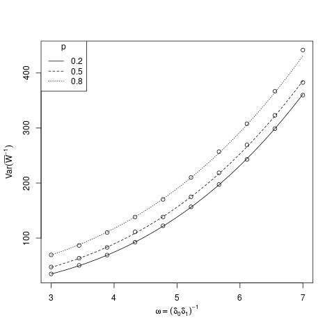
Figure 12: The second moment of the unstabilized IV weights in the two-state markov model. The effect of the known confounding, as measured by $p$, is small relative to the effect of the IV weakness, as measured by $1/(\delta_{0}\delta_{1})$. Another factor, the degree of known confounding of the IV, is fixed in this figure. The lines are the theoretical values and the plotted characters come from a Monte Carlo simulation. For the simulation the number of time points $T$ is 5 and the sample size $n$ is 50.

As with SRA weights, the function $h(\overline{A})$ in Theorem 1 may be chosen to partially stabilize IV weights. A function of $\overline{A}$ approximating $\Delta_{t}$ may be used to cancel out the magnitude of the weights and minimize the second moment of the weights. As in the SRA case, the influence function (20) does not change when $h$ is multiplied by a constant scalar, so the minimization is well-posed. Analogously to SRA weights, we consider stabilizing a weight term $\delta_{L_{t}}$ by an arbitrary term depending on the treatment previous to $L_{t}$, say, $\gamma_{A_{t-1}}$, with values $\gamma_{0},\gamma_{1}$. For example, analogous to the term $f(A_{t}\mid\overline{A}_{t-1})=\mathbb{E}(f(A_{t}\mid\overline{L}_{t},\overline{A}_{t-1})\mid\overline{A}_{t-1})$ commonly used to stabilize SRA weights, we may take

$$\gamma_{A_{t-1}} =\mathbb{E}(\delta_{L_{t}}\mid\overline{A}_{t-1})=\mathbb{E}(\delta_{L_{t}}\mid{A}_{t-1})=p_{L}\delta_{A_{t-1}}+(1-p_{L})\delta_{1-A_{t-1}},\hskip 14.45377ptt>1,$$

$$\gamma_{A_{0}} =\mathbb{E}(\delta_{L_{1}}\mid A_{0})=\mathbb{E}(\delta_{L_{1}}).$$

The squared inverse of the weights is

$$1/\overline{W}^{2}=\prod_{t}\gamma_{A_{t-1}}^{2}/\delta_{L_{t}}^{2}.$$

Proceeding as before, let

$$\phi_{t}(l_{t-1}) \coloneqq\mathbb{E}(\prod_{t^{\prime}=t}^{T}\gamma_{A_{t^{\prime}-1}}^{2}/\delta_{L_{t^{\prime}}}^{2}\mid L_{t-1}=l_{t-1}),\hskip 14.45377ptl_{t-1}\in\{0,1\},$$

$$\phi_{t} \coloneqq(\phi_{t}(0),\phi_{t}(1)).$$

Then $\mathbb{E}(1/\overline{W}^{2})=\gamma_{0}^{2}(\phi_{2}(0)/2+\phi_{2}(1)/2)$, $\phi$ satisfies the recurrence

$$\begin{aligned} \phi_{t-1}=\begin{pmatrix}p_{LA}p_{AL}\gamma_{0}^{2}/\delta_{0}^{2}+(1-p_{LA})(1-p_{AL})\gamma_{1}^{2}/\delta_{0}^{2}&p_{LA}(1-p_{AL})\gamma_{0}^{2}/\delta_{1}^{2}+p_{AL}(1-p_{LA})\gamma_{1}^{2}/\delta_{1}^{2}&\\ p_{LA}(1-p_{AL})\gamma_{1}^{2}/\delta_{0}^{2}+p_{AL}(1-p_{LA})\gamma_{0}^{2}/\delta_{0}^{2}&p_{LA}p_{AL}\gamma_{1}^{2}/\delta_{1}^{2}+(1-p_{LA})(1-p_{AL})\gamma_{0}^{2}/\delta_{1}^{2}\end{pmatrix}\phi_{t},\end{aligned}$$ (40)

and the growth of $\mathbb{E}(1/\overline{W}^{2})$ is determined by the eigenvalues of the matrix $P$ in (40),

$$\operatorname{tr}(P)/2\pm\sqrt{\operatorname{tr}(P)^{2}/4-\det(P)}$$

where

$$\operatorname{tr}(P) =p_{LA}p_{AL}(\gamma_{0}^{2}/\delta_{0}^{2}+\gamma_{1}^{2}/\delta_{1}^{2})+(1-p_{LA})(1-p_{AL})(\gamma_{0}^{2}/\delta_{1}^{2}+\gamma_{1}^{2}/\delta_{0}^{2})$$

$$\det(P) =(2p_{LA}-1)(2p_{AL}-1)\frac{\gamma_{0}^{2}\gamma_{1}^{2}}{\delta_{0}^{2}\delta_{1}^{2}}.$$

In terms of the IV weakness and confounding terms (39), the principal eigenvalue may be rewritten as

$$\lambda_{1}=\frac{1}{4}\left(\sqrt{\kappa^{2}+4\omega^{2}}(\gamma_{0}+\gamma_{1})(p_{LA}p_{AL}+(1-p_{LA})(1-p_{AL}))+\kappa(\gamma_{0}-\gamma_{1})(1-p_{LA}-p_{AL})\right)\times$$

$$\left(1+\sqrt{1-\frac{4\det(P)}{\operatorname{tr}(P)^{2}}}\right).$$

The last factor in parentheses has magnitude at most 2. As mentioned previously, it may be assumed without loss of generality that $\prod_{j}\gamma_{A_{j}}$ has expectation 1 for any law under which $\prod_{j}\gamma_{A_{j}}$ has finite expectation. For the variance of the influence function (20) does not change on multiplying $h(\overline{A})=h_{1}(\overline{A})\prod_{j}\gamma_{A_{j}}$ by a constant, so that any choice of $\prod_{j}\gamma_{A_{j}}$ may be replaced by another with mean 1, i.e., $\prod_{j}\gamma_{A_{j}}/\int\prod_{j}\gamma_{A_{j}}d\mu$. Letting $\mu$ be counting measure, the assumption becomes

$$1=\int\prod_{j}\gamma_{A_{j}}d\mu=\sum_{j=0}^{T}{T\choose j}\gamma_{0}^{j}\gamma_{1}^{T-j}=(\gamma_{0}+\gamma_{1})^{T}.$$

Therefore $\gamma_{0}+\gamma_{1}=1$ and the principal eigenvalue is

$$\lambda_{1}=\frac{1}{4}\left\{\sqrt{\kappa^{2}+4\omega^{2}}(p_{LA}p_{AL}+(1-p_{LA})(1-p_{AL}))+\kappa(\gamma_{0}-\gamma_{1})(1-p_{LA}-p_{AL})\right\}\left(1+\sqrt{1-\frac{4\det(P)}{\operatorname{tr}(P)^{2}}}\right).$$

Therefore, the effect of IV confounding $\kappa$ on the variance may be reduced by choosing $\gamma_{0}-\gamma_{1}$ close to 0, but no choice of $(\gamma_{0},\gamma_{1})$ will have an effect on the weakness of the IV, $\omega$, due to the term $\sqrt{\kappa^{2}+4\omega^{2}}$. See Fig. 13 for a simulation.

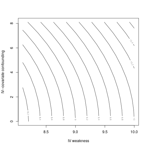
(a) Unstabilized IV weights

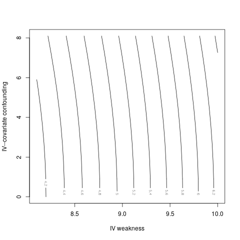
(b) Stabilized IV weights

Figure 13: The variance of the IV estimator depends on the weakness of the IV and the dependence of the IV on the covariates. An approximation to the variance is plotted against IV weakness and IV confounding using unstabilized and stabilized weights. The effect of IV confounding is mitigated by stabilization, but the effect of a weak IV remains.

Given below is a summary of the discussion of the asymptotic variance of the estimator in the four situations considered in this example.

1. SRA weights, unstabilized: The variance is exponential in $T$, and for fixed $T$ the variance blows up at a quadratic rate as the confounding $p_{LA}=\mathbb{P}(A\mid L)$ approaches $0$ or $1$.

2. SRA weights, stabilized: The variance is bounded as long as the confounding $p_{LA}=\mathbb{P}(A\mid L)$ is of the same order as the “predictiveness” $p_{AL}=\mathbb{P}(L\mid A)$.

3. IV weights, unstabilized: The variance of the weight terms is exponential in $T$, and for fixed $T$ is linear in a terms relating to the weakness of the IV and the degree of dependency between the IV and covariates.

4. IV weights, stabilized: The variance due to dependency between the IV and covariates may be reduced, but the variance due to the weakness of the IV remains.

The difference between the SRA and IV cases seems to be the following. In both cases the stabilization terms may be assumed to integrate to 1, due to the scale invariance property of the variance of the influence function mentioned earlier. In the case of SRA weights, the weights themselves also satisfy this type of property, being densities. Specifically, the terms $\prod_{t}f(a_{t}\mid l_{t-1})$ cannot be uniformly small across all choices $a_{t},l_{t-1},t=1,\ldots,T$. One may therefore hope to choose the stabilizing terms to match the magnitude of the corresponding weight terms. The IV weights do not satisfy this type of property, i.e., $\delta_{0}$ and $\delta_{1}$ may both be arbitrarily small at the same time, and no choice of $(\gamma_{0},\gamma_{1})$, which cannot both be small at the same time due to the scale invariance, will control the weights.

16 Appendix: Details for the simulation section

16.1 Data generation

Lemma 5 gives appropriate conditions on the endogenous noise term $\eta$ for sampling outcomes $Y=m(\overline{A})+\eta+\epsilon$ consistent with a MSMM model and the assumptions of Theorem 1. For example, we may sample outcomes as

$$\mathbb{E}(Y\mid\overline{A},\overline{Z},\overline{L},\overline{U}) =\sum_{t}\left(f_{t}(L_{t},U_{t})-\mathbb{E}(f_{t}(L_{t},U_{t})\mid\overline{A}_{t-1},\overline{L}_{t-1},\overline{U}_{t-1})\right)+m_{\beta}(\overline{A}),$$

$$(L_{t},U_{t}) \perp\!\!\!\perp\overline{Z}_{t}\mid\overline{ALU}_{t-1}$$

for arbitrary functions $f_{t}$, once we have chosen a sampling scheme for $(\overline{A},\overline{Z},\overline{L},\overline{U})$ satisfying the stated conditional indepndence assumption. We choose linear functions, so that outcome variables $Y$ are sampled as

$$Y =\sum_{t=0}^{T}(\tau_{t}(L_{t}-\mathbb{E}(L_{t}\mid\overline{ALU}_{t-1}))+\rho_{t}(U_{t}-\mathbb{E}(U_{t}\mid\overline{ALU}_{t-1})))+m_{\beta}(\overline{A})+\epsilon$$

$$=\sum_{t=0}^{T}(\tau_{t}(L_{t}-\mathbb{E}(L_{t}\mid\overline{ALU}_{t-1}))+\rho_{t}(U_{t}-\mathbb{E}(U_{t}\mid\overline{ALU}_{t-1})))+\beta_{0}+\beta_{1}\sum_{t}A_{t}+\epsilon,$$

with $\rho_{t},\tau_{t}\in\mathbb{R}$ and $\epsilon$ standard normal. We set $\rho_{t}=\tau_{t}=1$ in our simulation.

For $1\leq t\leq T$, $U_{t}$ is sampled as standard normal and $Z_{t}$ is bernoulli with success probability 1/2, all mutually independent, ensuring the IV assumptions. The treatments $A_{t}$ and covariates $L_{t}$ are sampled recursively as:

$$\begin{split}L_{t+1}&=\lambda_{0}+\lambda_{1}A_{t}+\epsilon_{t}\\ \Phi^{-1}(\Delta_{t+1})&=\Phi^{-1}\left(\mathbb{P}(A_{t+1}=1\mid\overline{L}_{t+1},\overline{U}_{t+1},\overline{A}_{t},\overline{Z}_{t},Z_{t+1}=1)\right.\\ &\qquad\left.-\mathbb{P}(A_{t+1}=1\mid\overline{L}_{t+1},\overline{U}_{t+1},\overline{A}_{t},\overline{Z}_{t},Z_{t+1}=0)\right)\\ &=\alpha_{0}+\alpha_{1}L_{t+1}\\ \mathbb{P}(A_{t+1}=1\mid\overline{A}_{t},\overline{Z}_{t+1},\overline{L}_{t+1},\overline{U}_{t+1})&=\Phi(\nu_{0}+\nu_{1}L_{t+1}+\nu_{2}U_{t+1})\times(1-\Delta_{t+1})+Z_{t+1}\times\Delta_{t+1}.\end{split}$$ (41)

Here, $\Phi$ denotes the standard normal CDF and $\epsilon_{t}$ are mutually independent standard normal variables. The models chosen for $A_{t}$ and $\Delta_{t}$ ensure that Assumption (8) holds. The parameters $\lambda_{0},\lambda_{1}\in\mathbb{R}$ control the extent to which the treatment confounds subsequent covariates, whereas $\nu_{1}\in\mathbb{R}$ and $\nu_{2}\in\mathbb{R}$ control the extent to which observed and unobserved confounders confounders, respectively, confound treatment. The reciprocal arrangement ensures that the confounding is truly longitudinal, so that, e.g., a series of propensity score analyses would not likely estimate the MSMM parameter accurately. The dependence between treatment and a confounder unavailable for estimation, provided $\nu_{2}\neq 0$, violates SRA. The parameters $\alpha_{0},\alpha_{1},$ bear on the strength of the IV. We set $\lambda_{0}=\lambda_{1}=.5,\alpha_{0}=\alpha_{1}=.3,\nu_{0}=-.2,$ and $\nu_{1}=\nu_{2}=.2$ in the simulation described below.

16.2 Estimation

As $f_{Z_{t}}$ is known under our data generation method (41), only $\beta,\alpha,$ and $\nu$ require estimation. We use (17) as an estimating equation for $\beta$ and obtain $\frac{\partial s_{\beta}}{\partial\beta,\alpha}$ from (21) by substituting

$$\frac{\partial}{\partial\beta}\mu(\beta)=\frac{\partial}{\partial\beta}\left(\beta_{0}+\beta_{1}\sum A_{t}\right)=(1,\sum A_{t})\text{ and }\frac{\partial}{\partial\alpha}\Delta_{t}(\alpha)=\frac{\partial}{\partial\alpha}\Phi(\alpha^{T}L_{t})=\phi(\alpha^{T}L_{t})L_{t}.$$

We use maximum likelihood to estimate $\alpha$ and $\nu$, pooling over the time points. After integrating out $U_{t}$, model (41) implies the observed-data model

$$\pi_{t}(\alpha,\nu)=\mathbb{P}(A_{t}=1\mid\overline{A}_{t-1},\overline{L}_{t},\overline{Z}_{t})=\Phi(\nu^{T}L_{t})(1-\Phi(\alpha^{T}L_{t}))+Z_{t}\Phi(\alpha^{T}L_{t}),$$

so that the conditional density of $A_{t}$ given the observed data is $\pi_{t}(\alpha,\nu)^{A_{t}}(1-\pi_{t}(\alpha,\nu))^{1-A_{t}}$, the scores for $\alpha$ and $\nu$ are

$$s(\alpha,\nu)=\left(\frac{A_{t}}{\pi_{t}(\alpha,\nu)}-\frac{1-A_{t}}{1-\pi_{t}(\alpha,\nu)}\right)\frac{\partial\pi_{t}(\alpha,\nu)}{\partial\alpha,\nu},$$

and the information is

$$\frac{\partial s(\alpha,\nu)}{\partial\alpha,\nu}=$$

$$\left(-\frac{A_{t}}{\pi_{t}(\alpha,\nu)^{2}}-\frac{1-A_{t}}{(1-\pi_{t}(\alpha,\nu))^{2}}\right)\frac{\partial\pi_{t}(\alpha,\nu)}{\partial\alpha,\nu}\left(\frac{\partial\pi_{t}(\alpha,\nu)}{\partial\alpha,\nu}\right)^{T}+\left(\frac{A_{t}}{\pi_{t}(\alpha,\nu)}-\frac{1-A_{t}}{1-\pi_{t}(\alpha,\nu)}\right)\frac{\partial^{2}\pi_{t}(\alpha,\nu)}{\partial(\alpha,\nu)^{2}}$$

with

$$\frac{\partial\pi_{t}(\alpha,\nu)}{\partial\alpha,\nu} =\left((Z_{t}-\Phi(\nu^{T}L_{t}))\phi(\alpha^{T}L_{t})L_{t},(1-\Phi(\alpha^{T}L_{t}))\phi(\nu^{T}L_{t})L_{t}\right)$$

$$\frac{\partial^{2}\pi_{t}(\alpha,\nu)}{\partial(\alpha,\nu)^{2}} =\begin{pmatrix}-(Z-\Phi(\nu^{T}L_{t}))\phi(\alpha^{T}L_{t})(\alpha^{T}L_{t})L_{t}L_{t}^{T}&-\phi(\nu^{T}L_{t})\phi(\alpha^{T}L_{t})L_{t}L_{t}^{T}\\ -\phi(\alpha^{T}L_{t})\phi(\nu^{T}L_{t})L_{t}L_{t}^{T}&-(1-\Phi(\alpha^{T}L_{t})\phi(\nu^{T}L_{t})(\nu^{T}L_{t})L_{t}L_{t}^{T}\end{pmatrix}.$$

The remaining entries of $\partial s/\partial(\beta,\alpha,\gamma,\nu)$ are 0. The “sandwich estimator” for the variance of $\hat{\beta}$ can then be computed as the empirical covariance matrix of (20).

A closed-form expression for the estimator $\hat{\beta}$ when the MSMM is linear, as in this example, is given in (18).

References

- Abadie (2003) Abadie, A. (2003). Semiparametric instrumental variable estimation of treatment response models. Journal of Econometrics 113(2), 231–263.
- Angrist et al. (1996) Angrist, J. D., G. W. Imbens, and D. B. Rubin (1996). Identification of causal effects using instrumental variables. Journal of the American statistical Association 91(434), 444–455.
- Baker and Lindeman (1994) Baker, S. G. and K. S. Lindeman (1994). The paired availability design: a proposal for evaluating epidural analgesia during labor. Statistics in Medicine 13(21), 2269–2278.
- Cerdá et al. (2010) Cerdá, M., A. V. Diez-Roux, E. T. Tchetgen, P. Gordon-Larsen, and C. Kiefe (2010). The relationship between neighborhood poverty and alcohol use: estimation by marginal structural models. Epidemiology (Cambridge, Mass.) 21(4), 482.
- Cook et al. (2002) Cook, N. R., S. R. Cole, and C. H. Hennekens (2002). Use of a marginal structural model to determine the effect of aspirin on cardiovascular mortality in the physicians’ health study. American Journal of Epidemiology 155(11), 1045–1053.
- Cui et al. (2020) Cui, Y., H. Michael, F. Tanser, and E. Tchetgen Tchetgen (2020). Instrumental variable estimation of marginal structural Cox models for time-varying treatments.
- Heckman and Urzua (2010) Heckman, J. J. and S. Urzua (2010). Comparing IV with structural models: What simple IV can and cannot identify. Journal of Econometrics 156(1), 27–37.
- Hernán et al. (2002) Hernán, M. A., B. A. Brumback, and J. M. Robins (2002). Estimating the causal effect of zidovudine on CD4 count with a marginal structural model for repeated measures. Statistics in medicine 21(12), 1689–1709.
- Imbens and Angrist (1994) Imbens, G. W. and J. D. Angrist (1994). Identification and estimation of local average treatment effects. Econometrica 62(2), 467–475.
- Lorch et al. (2012) Lorch, S. A., M. Baiocchi, C. E. Ahlberg, and D. S. Small (2012). The differential impact of delivery hospital on the outcomes of premature infants. Pediatrics 130(2), 270–278.
- Morrison et al. (2010) Morrison, C. S., C. Pai-Lien, K. Cynthia, B. A. Richardson, T. Chipato, R. Mugerwa, J. Byamugisha, N. Padian, D. D. Celentano, and R. A. Salata (2010). Hormonal contraception and hiv acquisition: reanalysis using marginal structural modeling. AIDS (London, England) 24(11), 1778.
- Richardson and Robins (2013) Richardson, T. S. and J. M. Robins (2013). Single world intervention graphs (SWIGs). Center for the Statistics and the Social Sciences, University of Washington Series. Working Paper 128(30), 2013.
- Robins (1997a) Robins, J. (1997a). Marginal Structural Models. In 1997 Proceedings of the American Statistical Association, pp. 1–10 of 1998 Section on Bayesian Statistical Science.
- Robins (1994) Robins, J. M. (1994). Correcting for non-compliance in randomized trials using structural nested mean models. Communications in Statistics-Theory and methods 23(8), 2379–2412.
- Robins (1997b) Robins, J. M. (1997b). Causal inference from complex longitudinal data. In Latent variable modeling and applications to causality, pp. 69–117. Springer.
- Robins (2000) Robins, J. M. (2000). Marginal structural models versus structural nested models as tools for causal inference. In Statistical models in epidemiology, the environment, and clinical trials, pp. 95–133.
- Tchetgen Tchetgen et al. (2018) Tchetgen Tchetgen, E. J., H. Michael, and Y. Cui (2018, September). Marginal Structural Models for Time-varying Endogenous Treatments: A Time-Varying Instrumental Variable Approach. ArXiv e-prints.
- VanderWeele et al. (2011) VanderWeele, T. J., L. C. Hawkley, R. A. Thisted, and J. T. Cacioppo (2011). A marginal structural model analysis for loneliness: implications for intervention trials and clinical practice. Journal of consulting and clinical psychology 79(2), 225.
- Wang and Tchetgen Tchetgen (2018) Wang, L. and E. Tchetgen Tchetgen (2018). Bounded, efficient and multiply robust estimation of average treatment effects using instrumental variables. Journal of the Royal Statistical Society: Series B (Statistical Methodology) 80(3), 531–550.
- Yang et al. (2014) Yang, F., S. A. Lorch, and D. S. Small (2014). Estimation of causal effects using instrumental variables with nonignorable missing covariates: application to effect of type of delivery NICU on premature infants. The Annals of Applied Statistics 8(1), 48–73.