Evolution of $Q$ Values for Deep Q Learning in Stable Baselines

Abstract

We investigate the evolution of the $Q$ values for the implementation of Deep Q Learning (DQL) in the Stable Baselines library. Stable Baselines incorporates the latest Reinforcement Learning techniques and achieves superhuman performance in many game environments. However, for some simple non-game environments, the DQL in Stable Baselines can struggle to find the correct actions. In this paper we aim to understand the types of environment where this suboptimal behavior can happen, and also investigate the corresponding evolution of the $Q$ values for individual states.

We compare a smart TrafficLight environment (where performance is poor) with the AI Gym FrozenLake environment (where performance is perfect). We observe that DQL struggles with TrafficLight because actions are reversible and hence the $Q$ values in a given state are closer than in FrozenLake. We then investigate the evolution of the $Q$ values using a recent decomposition technique of Achiam et al. [1]. We observe that for TrafficLight, the function approximation error and the complex relationships between the states lead to a situation where some $Q$ values meander far from optimal.

1 Introduction

Deep Q Learning (DQL) has recently emerged as a powerful way to learn optimal actions in high-dimensional state spaces that are not addressable by conventional Reinforcement Learning (RL) techniques. DQL aims to learn a $Q$ function that represents the long-term discounted reward from taking each action. The “deep” part of the DQL name refers to the fact that we aim to train a Deep Neural Network to approximate this $Q$ function.

Despite its practical successes in game environments such as Chess and Go [2], a theoretical description of how the $Q$ values evolve for any given environment is a challenge. As with any DNN-based function approximation we need to understand how the DNN generalizes to inputs on which it has not been trained [3]. However, DQL has an additional feedback effect in that the output of the DNN at one step feeds back into the state reached at the next time step. This provides an additional difficulty in understanding its behavior.

In this paper we study the detailed evolution of the $Q$ values for the DQL implementation in Stable Baselines [4]. Stable Baselines is a python library for RL that is a fork of the earlier AI baselines library [5]. It supports many Deep Reinforcement Learning algorithms and is becoming the standard implementation for many of them [6] as it incorporates all of the latest improvements from the academic literature. The Stable Baselines DQL implementation has spectacular (and superhuman) performance for standard RL environments such as AI Gym Atari games [7]. For example, it achieves perfect learning for the Pong game where the state is simply the pixel representation of the game image.

Despite this performance on games, we show that even for the state-of-the-art implementation of DQL in Stable Baselines, we can sometimes get tripped up by simple environments modeling real-world RL applications. We investigate an environment for smart traffic lights where the $Q$ values do not converge to the correct values and we do not get the correct action for all states. Our goal is to investigate what makes this environment difficult for DQL and to understand the detailed evolution of the $Q$ values and why they do not reach the “correct” values.

We remark that our environments are simple enough that they do not require DQL. In particular, we know the optimal $Q$ values because we can run standard value iteration across all state/action pairs. However, we prefer to focus on simple examples since it allows us to analyze the $Q$-value evolution for a meaningful fraction of individual states. Similarly, rather than contrasting the TrafficLight problem with a complex “good” example such as Pong, we use a much simpler good example from the AI Gym called FrozenLake. By obtaining a detailed understanding of DQL behavior on these small examples, we can gain a better sense of when DQL might struggle on much larger environments where non-DNN-based RL methods would not be practical.

1.1 Results and Paper Organization

In Section 1.2 we introduce Q-Learning and the DQL framework, in Section 1.3 we introduce the FrozenLake and TrafficLight environments that we focus on, in Section 1.4 we briefly describe Stable Baselines and in Section 1.5 we discuss related work. In Section 2 we describe how the performance of DQL on the game-like FrozenLake is superior to the performance on the non-game-like TrafficLight. In particular, actions in TrafficLight are more reversible. This implies that there is no such thing as a “terrible” action in TrafficLight which in turn makes it harder to find the action with the best long-term reward.

In the remainder of the paper we discuss the evolution of the $Q$-values and discuss why DQL does not find the optimal $Q$ values for TrafficLight. In Section 3 we describe the framework of Achiam et al. [1] that decomposes the $Q$-value using the Neural Tangent Kernel matrix. Using this decomposition as a guide, we distinguish between updates when the associated state is used for training and updates when it is not (and hence the update is based on the DNN generalization). In Section 4 we use this framework to analyze our environments. We examine the $Q$-value updates and temporal difference errors for individual states. We observe that although the $Q$ values for a state/action pair do move in the correct direction (on average) when we train on that pair, the overall adjustments (including steps where we do not train on the pair) are too noisy to bring the $Q$ value to the correct point.

1.2 Model and Terminology

We consider the standard setting of Reinforcement Learning. We assume an agent interacting with an environment. Let $S$ be the state space and let $A$ be the action space. The problem is governed by the transition and reward functions.

• The transition $P(s,a,s^{\prime})$ represents the probability that we transition to state $s^{\prime}$ after taking action $a$ in state $s$.

• The reward $R(s,a)$ is the instantaneous reward that the agent receives for taking action $a$ in state $s$.

The goal is to maximize the infinite-horizon discounted reward. In particular, if $Q^{*}(\cdot,\cdot)$ satisfies the Bellman equation,

$$Q^{*}(s,a)=E_{s\rightarrow s^{\prime}}[R(s,a)+\max_{a^{\prime}}Q^{*}(s^{\prime},a^{\prime})],$$

then we refer to $Q^{*}(\cdot,\cdot)$ as the optimal action-value function. The goal is to compute this function and then always choose the action $\max_{a}Q^{*}(s,a)$ in state $s$.

In the Reinforcement Learning literature, three basic methods for computing $Q^{*}(\cdot,\cdot)$ in an iterative fashion are typically considered. In the sequel we follow the notation of [1].

• In value iteration, we update the $Q$ value for all state-action pairs in each iteration. In particular, let $T^{*}$ be the operator defined by the right-hand side of the Bellman equation,

  $$(T^{*}Q)(s,a)=E_{s\rightarrow s^{\prime}}[R(s,a)+\max_{a^{\prime}}Q(s^{\prime},a^{\prime})].$$

  Then value iteration updates $Q$ according to $Q_{k+1}=T^{*}Q_{k}$. By the Banach fixed point theorem, value iteration converges to the optimal solution $Q^{*}$ that satisfies $Q^{*}=T^{*}Q^{*}$. The difference $|T^{*}Q_{k}(s,a)-Q_{k}(s,a)|$ is the expected temporal difference error (TD-error) for state/action pair $(s,a)$ at iteration $k$.

• In regular Q-learning [8], we visit states according to the current values of $Q$ and only update $Q$ for the states that are visited. Let $(s_{0},a_{0}),(s_{1},a_{1}),\ldots$ be the sequence of state-action pairs that are visited. Then at iteration $k$ we update according to:

  $$Q_{k+1}(s_{k},a_{k})=(1-\alpha_{k})Q_{k}(s_{k},a_{k})+\alpha_{k}(R(s_{k},a_{k})+\gamma\max_{a^{\prime}}Q_{k}(s_{k+1},a^{\prime})),$$

  for some sequence of learning rates $\alpha_{k}$. The difference $(R(s_{k},a_{k})+\gamma\max_{a^{\prime}}Q_{k}(s_{k+1},a^{\prime}))-Q_{k}(s_{k},a_{k})$ is the realized temporal difference error at iteration $k$. We keep $Q_{k+1}(s,a)=Q_{k}(s,a)$ for all $(s,a)\neq(s_{k},a_{k})$.

• In Deep Q-learning, the Q function is parameterized by a vector $\theta$ (that can be the weights of a Deep Neural Network). We update $\theta$ according to:

  (1) $$\theta_{k+1}=\theta_{k}+\alpha_{k}(R(s_{k},a_{k})+\gamma\max_{a^{\prime}}Q_{\theta_{k}}(s_{k+1},a^{\prime})-Q_{\theta_{k}}(s_{k},a_{k}))\nabla_{\theta}Q_{\theta_{k}}(s_{k},a_{k}).$$

1.3 Two Environments

Although Deep Q-Learning makes the most sense for large state spaces, the goal of this paper is to investigate how the function approximation associated with the neural network can prevent convergence to the optimal $Q$ values, even for “toy” state spaces. We now define two such environments.

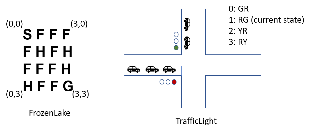
Figure 1: The FrozenLake and TrafficLight environments.

FrozenLake is one of the simplest environments in the AI Gym [9]. It is essentially a maze problem defined by the map in Figure 1 (left). The goal is to travel from start state $S$ to goal state $G$ across a frozen lake. States marked $F$ are “frozen” states that can support our weight. States marked $H$ are “hole” states that lead to us falling into the lake. At all times we can take actions from the set $\{L,D,R,U\}$ corresponding to the directions left, down, right, up. (There is no wraparound and so if we try to move left in state $S$ then we stay in state $S$.) When we reach a termination state in $\{H,G\}$ then we stay in that state indefinitely. The reward $R(s,a)$ is $1$ if $s$ is the goal state $G$ and $0$ otherwise.

The slipperiness of the ice means that we do not always move in the direction selected. Taking action $L$ leads to actual movement in $\{U,L,D\}$ (each with probability $1/3$). Action $D$ leads to actual movement in $\{L,D,R\}$, action $R$ leads to actual movement in $\{D,R,U\}$ and action $U$ leads to actual movement in $\{R,U,L\}$.

We will see that DQL works extremely well on this simple FrozenLake environment. This is in contrast to the equally simple TrafficLight environment that we describe next.

TrafficLight.

The control of smart traffic systems has been viewed in many works as a likely application area of DQL [10]. In these systems the goal of DQL is to make traffic light decisions based on where the cars are waiting. We focus on an extremely simple version of TrafficLight with 2 car lanes, a horizontal lane and a vertical lane. See Figure 1 (right). The state of the traffic light goes in a cycle $GR\rightarrow YR\rightarrow RG\rightarrow RY\rightarrow GR\ldots$. The numerical coding of the states is given in the figure. If the light is in state $GR=0$ then 1 car is served from the queue of horizontal cars. If the light state is $RG=1$ then 1 car is served from the queue of vertical cars. If the light state is $YR=2$ or $RY=3$ then neither queue is served. In order to make the state space finite we assume a cap $q_{\max}$ on each queue size. For every time step in which a queue has fewer than $q_{\max}$ cars, a new car arrives into the queue with probability $p$.

At each time step the actions available to the light are continue and switch. If continue is chosen then the light state is the same at the next time step. If switch is chosen then the light advances to the next state in the above cycle. Let $q_{H}$ (resp. $q_{V}$) denote the number of cars in the horizontal (resp. vertical) queue. The state of the system is then given by $(q_{H},q_{V},\ell)$ where $\ell$ denotes the light state. The reward function is $r(q_{H},q_{V})=-q_{H}^{2}-q_{V}^{2}$ which encourages the queues to be small and balanced. If balancing the queues involves changing the light state then we must trade off the eventual improvement in the reward with the fact that we do not serve any queue when we are transitioning through the $YR$ and $RY$ starts. DQL is expected to handle this tradeoff since its objective is the discounted future reward.

1.4 Stable Baselines

Once a problem has been identified as an instance of RL, we ideally want to apply a DQL algorithm “out-of-the-box” to learn optimal performance. Stable Baselines [4] is emerging as the most widely used instantiation of DQL. It is a fork of an earlier package called AI Baselines [5] and it uses Tensorflow to construct the Deep Neural Network that is used to approximate the $Q$-function. Stable Baselines implements a comprehensive suite of modern RL algorithms. In this paper we focus on DQL since it is the most widely studied “Deep” Reinforcement Learning algorithm.

Stable Baselines utilizes many standard enhancements to the basic update rule described in Equation 1. First, it employs experience replay and minibatch gradient descent. Specifically, it stores the last $S$ states and rewards for some replay parameter $S$. Then at each iteration it extracts $b$ elements from the store, for some batch parameter $b$, and uses learning on those elements to update $\theta$. Second, it uses double Q learning so that two $Q$ functions are maintained. The first function, which we denote by $Q^{\prime}$, is used on the right hand side of the Bellman equation and is held fixed for $\tau$ iterations, for some parameter $\tau$. The second function $Q$ is updated every iteration according to the learning and is used to decide on the actions. At the end of each set of $\tau$ iterations, $Q^{\prime}$ is made equivalent to $Q$. The third enhancement is dueling DQL [11] in which the $Q$ function is divided into two components. The first component learns a value that depends on the state only, and the second learns how the value differs for each action. These components are learned by separate (but connected) neural networks.

Stable Baselines supports arbitrary neural networks for learning the $Q$ function. We use the default option which is a Multilayer Perceptron with 2 hidden layers of 64 nodes.

1.5 Related Work

François-Lavet et al. provide an extensive overview of Deep Reinforcement Learning techniques [12]. Some conditions that allow us to bound the error of $Q$ values in DQL were derived by Yang et al. in [13]. A number of papers have examined how $Q$ values are affected by function approximation. Fujimoto et al. [14] quantified overestimation bias while Fu et al. [15] isolated the effects of batch sampling and replay buffers and observed that larger neural networks have better performance, despite the danger of overfitting. Van Hasselt et al. [16] showed that the so-called “deadly triad” (bootstrapping, off-policy learning and function approximation) can lead to divergence of $Q$ values. A theoretical framework to understand this phenomenon was provided by Achiam et al. [1]. In Section 4 we use this framework to understand the observed evolution of $Q$ values in Stable Baselines. However, we remark that for our case we do not observe divergence (which typically is due to poor behavior in the early iterations). We instead study a situation where the $Q$ values do not diverge but they remain away from optimal. Other papers that address the behavior of DQL include [17, 18, 19].

2 Optimal vs learned $Q$ values

We begin with a high-level comparison of the performance of the Stable Baselines DQL implementation on FrozenLake and TrafficLight. Figure 1 (right) gives the optimal $Q$ values for FrozenLake. (The environment is small enough that we can compute the optimal values via value iteration.) The optimal action (with the largest $Q$ value) is in bold in each state (with multiple entries in bold in case of a tie). We remark that the optimal $Q$ values are less than $100$ for all except the goal state as a result of the discount factor $\gamma$. Figure 1 (left) shows the corresponding learned $Q$ values after the Stable Baselines DQL implementation is run for 350000 iterations. We see that most $Q$ values are close to optimal, especially for the state/action pairs that are actually selected (the entries in bold).

	learned				optimal
state	L	D	R	U	L	D	R	U
(0,0)	56.9	56.4	56.8	54.0	53.6	52.3	52.3	51.71
(1,0)	37.5	43.3	38.6	52.9	34.0	33.1	31.7	49.4
(2,0)	48.0	46.0	43.5	49.6	43.4	42.9	42.0	46.6
(3,0)	36.0	42.5	42.1	47.2	30.3	30.3	29.9	45.2
(0,1)	57.8	40.2	37.8	34.4	55.3	37.6	37.0	35.95
(1,1)	2.8	2.3	2.7	-0.0	0.0	0.0	0.0	0.00
(2,1)	40.1	38.0	40.6	23.2	35.5	20.1	35.5	15.4
(3,1)	-0.7	-2.1	-4.9	1.0	0.0	0.0	0.0	0.00
(0,2)	41.4	50.0	44.5	61.8	37.6	40.3	39.3	58.6
(1,2)	44.5	67.3	51.8	48.2	43.6	63.67	44.3	39.4
(2,2)	61.8	51.5	45.0	30.0	60.9	49.2	39.9	32.7
(3,2)	2.5	2.4	2.5	0.8	0.0	0.0	0.0	0.0
(0,3)	-2.4	-4.5	-6.9	-0.8	0.0	0.0	0.0	0.0
(1,3)	53.5	67.5	76.9	42.8	45.2	52.4	73.4	49.2
(2,3)	74.5	87.6	80.8	76.4	72.5	85.4	81.3	77.3
(3,3)	99.5	99.8	96.1	101.1	100	100	100	100

Table 1: Learned and optimal $Q$ values for FrozenLake. The state is denoted by $(x,y)$ where $(0,0)$ corresponds to the top left start state. The “hole” states are $(1,1)$, $(3,1)$, $(3,2)$ and $(0,3)$.

In contrast we now examine a subset of the Q-value table for the TrafficLight environment with a maximum queue size of 5 cars and an arrival rate $p=0.45$ for each queue. (We do not include the whole table for reasons of space.) The right columns of Figure 2 have the optimal values and the left columns have the learned values after running the Stable Baselines implementation of DQL with default parameters for $1000000$ iterations. We see that for some states (e.g. $(0,1,0)$ and $(0,2,0)$), the ordering of the actions switch/continue based on $Q$ value are incorrect compared to the optimal values. Moreover, even for states where the ordering is correct, the $Q$ values are far from optimal.

	learned		optimal
state	Switch	Continue	Switch	Continue
(0, 1, 0)	-1176.4	-774.6	-1431.2	-1438.0
(0, 1, 3)	-977.7	-1374.3	-1438.0	-1457.0
(0, 2, 0)	-1242.9	-1138.8	-1472.3	-1490.1
(0, 2, 1)	-1234.1	-929.0	-1457.0	-1410.0
(1, 0, 1)	-1025.6	-1152.0	-1431.2	-1438.0
(1, 5, 0)	-1524.8	-1548.9	-1613.7	-1623.0
(2, 0, 0)	-1288.0	-762.5	-1457.0	-1410.0
(2, 2, 0)	-1391.7	-1303.1	-1533.4	-1509.2
(2, 2, 1)	-1406.4	-1333.3	-1533.4	-1509.2
(2, 3, 2)	-1566.9	-1582.4	-1601.7	-1652.1
(3, 4, 0)	-1625.6	-1572.3	-1706.1	-1647.6
(4, 2, 1)	-1584.9	-1565.9	-1650.0	-1617.2
(4, 3, 2)	-1644.6	-1664.4	-1686.0	-1729.3
(4, 5, 0)	-1650.7	-1596.3	-1773.4	-1697.8
(5, 0, 0)	-1509.0	-1486.2	-1622.4	-1538.2
(5, 4, 0)	-1680.4	-1615.8	-1779.5	-1737.2

Table 2: Learned and optimal $Q$ values for TrafficLight for a sample of states.

We will see in Section 4 that the gap between the learned and optimal $Q$ values is not decreasing as we reach 1000000 iterations and so simply running for more iterations is unlikely to improve the solution. The goal of this paper is to gain a deeper understanding of why the Stable Baselines DQL implementation behaves differently in the two environments. We break this study into two questions.

• The simpler question that we address next is: Why does the inaccuracy in learning the $Q$ values lead to suboptimal action choices for TrafficLight?

• The more complex question that we address in Sections 3 and 4 is why the $Q$ values do not converge to optimal.

The immediate answer to the first question is that for TrafficLight, the $Q$ values for the different actions in a given state do not vary much. As a result the learned $Q$ values need to be highly accurate in order to achieve the correct actions. This has been noted before. Indeed, one of the main motivations of Dueling Deep Q Networks [11] (a technique employed by Stable Baselines) is to more carefully arbitrate between the actions for a given state.

In our context this creates a natural follow-up question: Why are the optimal $Q$ values for a given state close to each other? The answer comes from the intended meaning of $Q$ values. They are meant to represent the long-term reward gained from taking an action and then following the optimal policy from that point on. In the case of TrafficLight, these values cannot be too different since if we take the “wrong” action, we can always recover by quickly cycling the traffic light to a subsequent light state. (If we choose continue but the best action is switch, then we can switch at the next time step. If we choose switch but the best action is continue, then it only takes at most 3 steps to get back to the previous light state.) As a result, there is no such thing as a “terrible” action to take in a given state.

In contrast, in FrozenLake there are terrible actions to take. If we move into a hole when no such move is necessary, that would be a terrible action since once we are in a hole, the long-term reward is $0$. More generally, environments based on games often have such terrible actions. For example, in chess placing the queen in danger of capture without compensation would be regarded as a terrible action. Reinforcement Learning has had its greatest successes in game-like settings because in games there is often a significant difference in outcome between actions in a given state. This in turn leads to differences in $Q$ values and so DQL can identify the correct action, even if the $Q$ values do not converge all the way to optimal.

We remark that even if $Q$ values are similar for different actions in each state, it does not necessarily mean that any policy will lead to the same long-term outcome. The optimal $Q$ value for an $(s,a)$ pair represents the discounted reward for taking action $a$ in state $s$, followed by the optimal sequence of actions from that point on. It does not represent the long-term reward if we continue to take wrong actions over a long time period. Small differences in reward can aggregate over time. Hence getting good convergence for the $Q$ values is important even if the optimal $Q$ values are close together for each state. In the remainder of the paper we study the evolution of the $Q$ values in more detail.

3 Decomposition of DQL updates

We aim to explain the behavior of the $Q$ values using the framework of Achiam et al. [1] that decomposes the $Q$ value updates into 3 components that capture different aspects of the process. This framework was used in [1] to explain why DQL could sometimes diverge. However, we also find it a useful way to measure why the $Q$ values for TrafficLight end up at the wrong values (even though they do not diverge). The presentation of [1] is as follows for a simple version of DQL which does not use target or dueling networks, but does use a replay buffer. For this case the update of the DQL parameters is described by,

$$\theta_{k+1}=\theta_{k}+\alpha_{k}E_{(s,a)\sim\rho_{k}}[(R(s,a)+\gamma\max_{a^{\prime}}Q_{\theta_{k}}(s,a^{\prime})-Q_{\theta_{k}}(s,a))\nabla_{\theta}Q_{\theta_{k}}(s,a)],$$

where $\rho_{k}$ represents the distribution of state/action pairs in the replay buffer at step $k$. Combining this expression with the Taylor expansion for $Q_{\theta_{k}}(s,a)$ around $\theta_{k}$, we obtain,

$$Q_{\theta_{k+1}}(\bar{s},\bar{a})-Q_{\theta_{k}}(\bar{s},\bar{a})=\alpha_{k}E[\nabla_{\theta_{k}}Q_{\theta_{k}}(\bar{s},\bar{a})^{T}\nabla_{\theta_{k}}Q_{\theta_{k}}(s,a)(T^{*}Q_{\theta_{k}}-Q_{\theta_{k}})(s,a)]+O(||\theta_{k+1}-\theta_{k}||^{2}).$$

Dropping the second order term and vectorizing across states we write:

(2) $$Q_{\theta_{k+1}}\approx Q_{\theta_{k}}+\alpha_{k}K_{\theta_{k}}D_{\rho_{k}}(T^{*}Q_{\theta_{k}}-Q_{\theta_{k}}),$$

where $K_{\theta_{k}}$ is a matrix whose $((\bar{s},\bar{a}),(s,a))$ entry is given by $\nabla_{\theta_{k}}Q_{\theta_{k}}(\bar{s},\bar{a})^{T}\nabla_{\theta_{k}}Q_{\theta_{k}}(s,a)$ and $D_{\rho_{k}}$ is a diagonal matrix with entries given by $\rho_{k}(s,a)$. The matrix $K_{\theta_{k}}$ is known as the Neural Tangent Kernel (NTK) at $\theta_{k}$ [20].

Let us now interpret the decomposition in (2). The difference $T^{*}Q_{\theta_{k}}-Q_{\theta_{k}}$ is the vector of temporal differences at iteration $k$. If the $Q$ values are updated according to $Q_{\theta_{k+1}}=Q_{\theta_{k}}+\alpha_{k}(T^{*}Q_{\theta_{k}}-Q_{\theta_{k}})$ then we simply have a variant of value iteration in which the speed of update at each iteration is controlled by the $\alpha_{k}$ parameters. This will eventually converge since the $T^{*}$ operator is a contraction.

If however we use $Q_{\theta_{k+1}}=Q_{\theta_{k}}+\alpha_{k}D_{\rho_{k}}(T^{*}Q_{\theta_{k}}-Q_{\theta_{k}})$ then the update is an averaged version of regular $Q$ learning where we only update the $Q$ values for the states that are actually visited. Hence we should still obtain convergence to optimal $Q$ values.

Any errors therefore are due to the introduction of the NTK matrix $K_{\theta_{k}}$ into the update rule, and the interaction of $K_{\theta_{k}}$ with $D_{\rho_{k}}$ and $(T^{*}Q_{\theta_{k}}-Q_{\theta_{k}})$. In particular, the entries of $K_{\theta_{k}}$ indicate the level of generalization due to learning via the DNN. Achiam et al. [1] show that if $K_{\theta_{k}}$ has large diagonal entries and small off-diagonal entries, the DQL behaves well since its behavior tracks that of regular $Q$-learning. The paper then introduces a preconditioning term to the $Q$-value updates whose goal is to ensure that $K_{\theta_{k}}D_{\rho_{k}}(T^{*}Q_{\theta_{k}}-Q_{\theta_{k}})(s,a)$ is close to the TD-error $(T^{*}Q_{\theta_{k}}-Q_{\theta_{k}})(s,a)$ for state/action pairs $(s,a)$ that are sampled from the replay buffer. (They assume that multiple state/action pairs are sampled at each iteration.) They then show that this preconditioning improves the behavior of the $Q$-values for standard AI Gym environments, even in the absence of standard techniques such as target networks.

We remark however that having a large ratio between on-diagonal and off-diagonal entries in the NTK is a double-edged sword. Although it will improve the convergence of the $Q$-values, the smaller amount of generalization takes away many of the benefits of using the DNN for fast learning in large state spaces. Indeed, if $K_{\theta_{k}}$ is the identity matrix then we revert back to standard $Q$ learning, which will always converge to the optimal $Q$ values but which will be impractical for many large state spaces.

We therefore focus on understanding the out-of-box behavior produced by the Stable Baselines DQL implementation. We also consider a different question from [1] which looked at divergence of $Q$ values starting from the initial state. (They therefore focus on the structure of the NTK in the initial iterations.) In contrast, we are interested in explaining why the $Q$-values in TrafficLight do not reach the optimal values even though they do not diverge. For this we have to consider the entire evolution of the $Q$-values. Another difference in our work is that [1] do not characterize the types of environments where DQL has poor performance. Our comparison of FrozenLake and TrafficLight suggests that poor performance can occur when the range of $Q$ values in a given state is small.

Despite these differences, we find the high-level strategy of [1] to be an extremely useful tool in evaluating the evolution of the $Q$ values. Moreover, [1] highlight the relative absence of work on the NTK $K_{\theta}$. In the remainder of the paper we examine how the learned $Q$-values for different state/action pairs compare to the optimal values in our two environments. For state/action pairs that misbehave we compare the updates of the corresponding $Q$ values with the updates that would occur if we simply used the TD-error as in regular $Q$-learning.

4 Evolution of $Q$ values

The remainder of the paper examines the evolution of the $Q$-values for both FrozenLake and TrafficLight. Our goal is to understand why we do not converge to the correct solution for TrafficLight. All plots use the default parameters for DQL in Stable Baselines. The most important of these are: discount factor $\gamma=0.99$, learning rate $\alpha_{k}=0.0005$, replay buffer size$=50000$ and a batch size of $32$ sampled from the replay buffer at each iteration. The exploration fraction (i.e. the fraction of steps where we take a random action rather than the argmax of the $Q$ values) decreases from $100\%$ to $2\%$ over the first $10\%$ of the run. The target network is updated every 500 iterations. The plots show performance over $15$ runs (of $500000$ iterations for FrozenLake and $1000000$ iterations for TrafficLight) with error bars showing the variation between runs. In general, the qualitative behavior of both FrozenLake and TrafficLight is similar across runs. We have also varied the DQL hyperparameters but we omit those results for reasons of space. In particular, the performance is sensitive to batch size but we have not found hyperparameters where TrafficLight performs well. We run our experiments on a LambdaQuad machine running Ubuntu 18.04 with 32 16-core 2GHz CPUs.

We begin with FrozenLake. Let $Q_{opt}$ be the optimal $Q$ values. (For our small environments these can be computed directly from value iteration.) We can think of $Q$ and $Q_{opt}$ as vectors with one entry for each state/action pair. Figure 2 shows the evolution of $||Q-Q_{opt}||$. We see a clear pattern of learning taking place. Over the first $75000$ steps the value of $||Q-Q_{opt}||$ drops significantly and then it stabilizes for the remaining steps.

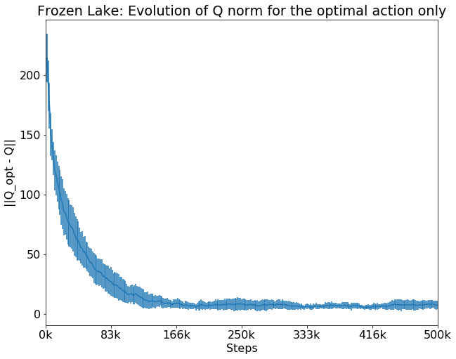
Figure 2: The difference between $Q$ and $Q^{opt}$ for FrozenLake.

We break this down in Figures 3(a) and 3(b) where we show the evolution of the $Q$ values across all 4 actions for states $1=(1,0)$ and $14=(3,2)$ respectively. We see that in both states the $Q$ value for the optimal action ($U$ for state 1 and $D$ for state 14) quickly becomes the maximum for that state and quickly approach the optimal value. The order of the suboptimal actions in state $1$ is not correct but this is because these states are rarely selected and so DQL rarely trains for those actions. However, the $Q$ values for the suboptimal actions do not rise above the $Q$ values for the optimal actions and so we obtain the correct decisions in these states.

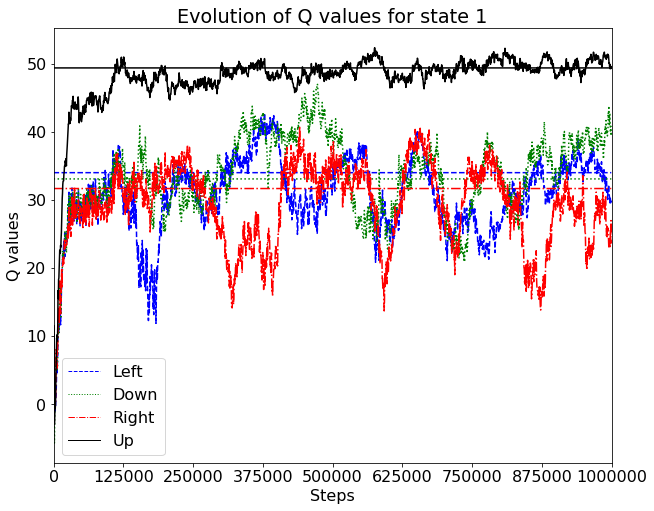
(a) State $1$.

(b) State $14$.

Figure 3: Evolution of $Q$ values for FrozenLake states $1$ and $14$.

We next consider TrafficLight. Figure 4 shows the evolution of $||Q-Q_{opt}||$. We see that unlike in FrozenLake, the difference between $Q$ and $Q_{opt}$ first decreases but then starts to increase after roughly 125000 iterations. We now consider some individual states to understand how their $Q$ values evolve. Recall that we denote the state using $(q_{H},q_{V},\ell)$ where $\ell$ is the traffic light state in $\{0,1,2,3\}=\{GR,RG,YR,RY\}$.

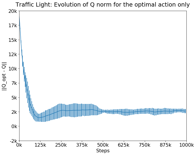
Figure 4: The difference between $Q$ and $Q^{opt}$ for TrafficLight.

Figure 6 shows the training frequency for the top 35 visited states. Figure 6 shows the optimal $Q$ values (green) vs the learned $Q$ values after 1000000 iterations (black - with red error bars) for the top visited states. We see that for many of these states the learned $Q$ values are significantly different from optimal. Figure 7 shows the $Q$-value evolution for state $(0,2,0)$. In this state queue $0$ is being served since the light state is $GR$. However, it is clear that the optimal solution is to switch (via state $2$) to serving queue $1$. Indeed, Figure 7 shows that the optimal $Q$ value for switch is larger than the optimal $Q$ value for continue. However, both of the learned $Q$ values deviate from their optimal values over the course of the learning, and the $Q$ value for continue is significantly above the $Q$ value for switch.

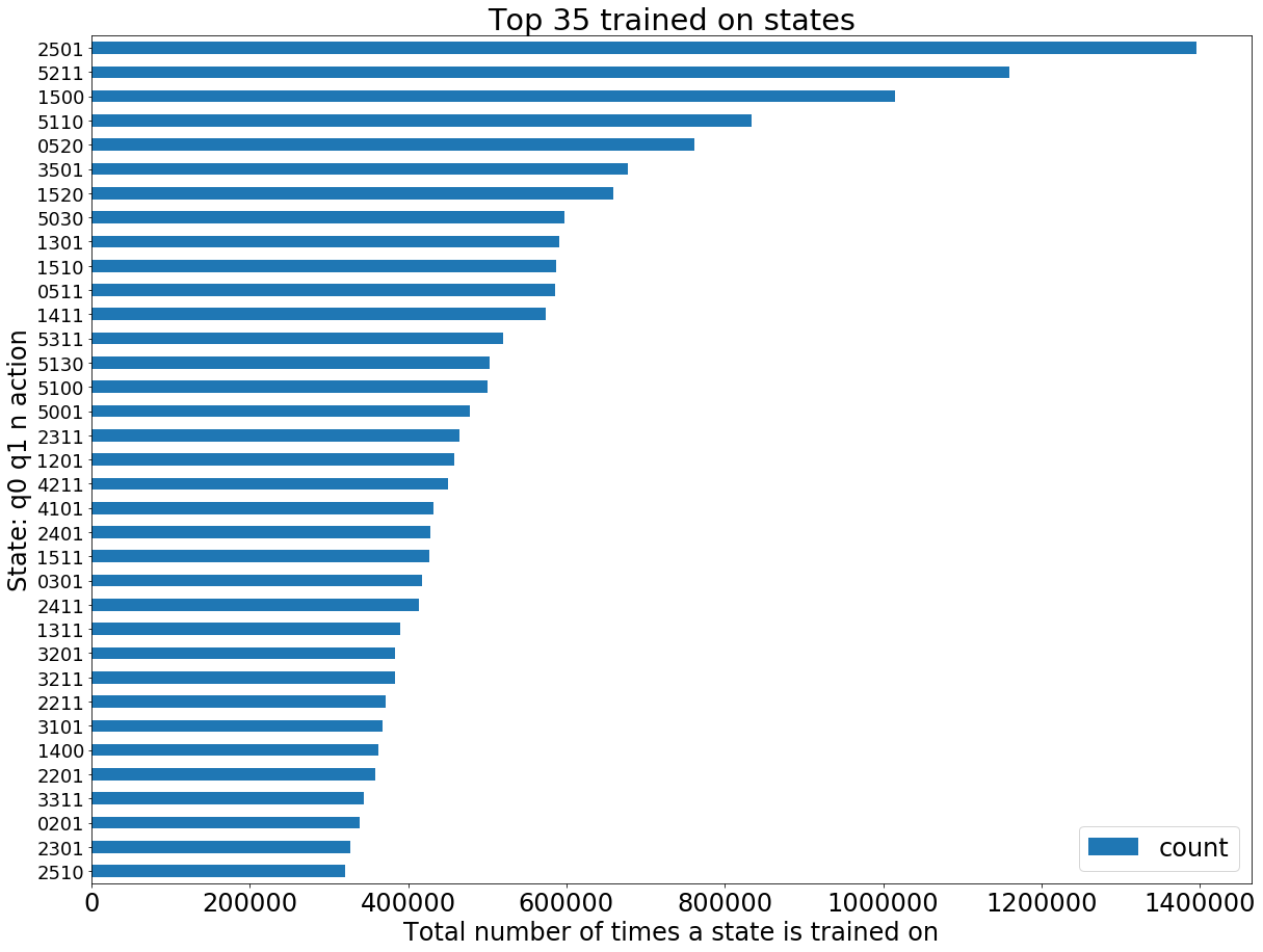
Figure 5: The top 35 visited states.

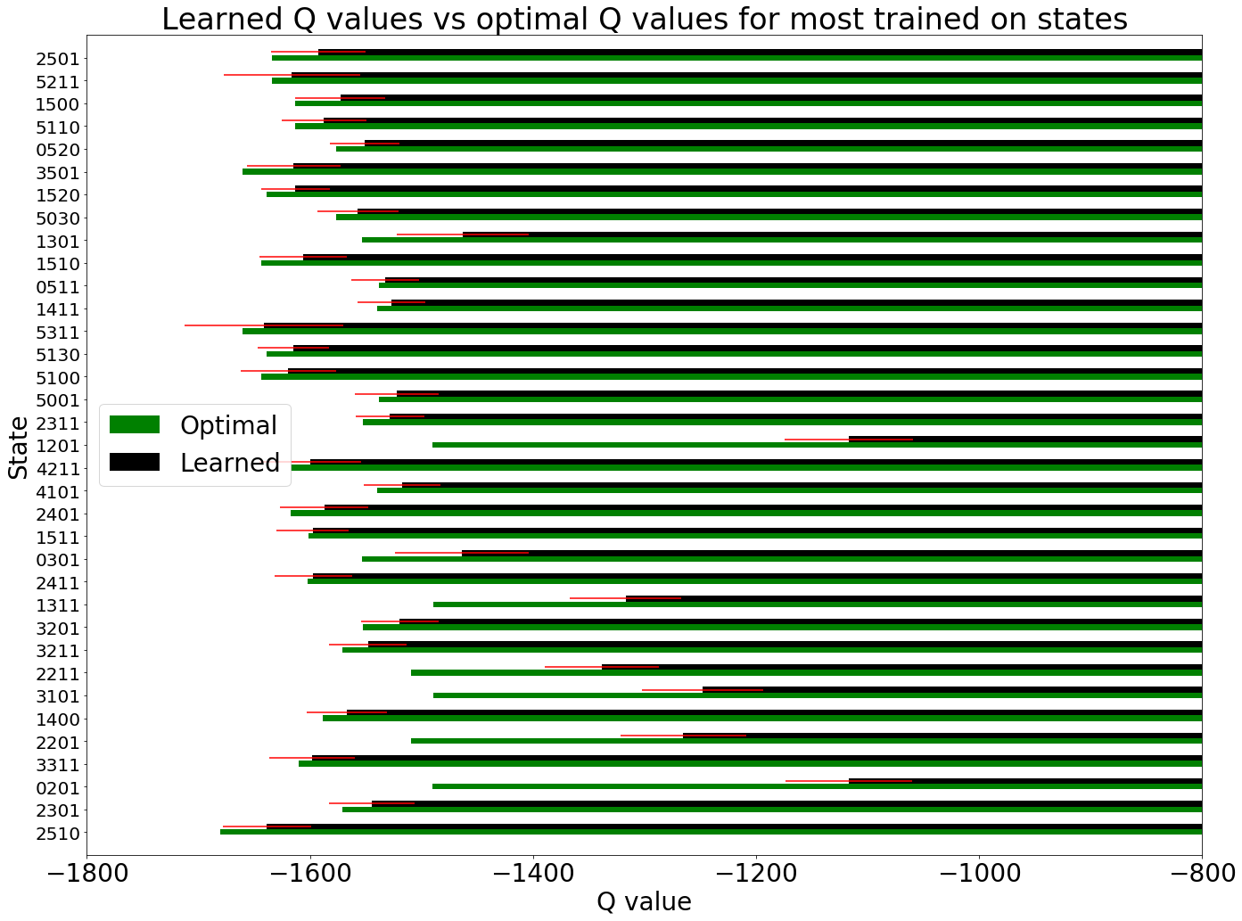
Figure 6: Optimal vs learned $Q$ values for
frequently visited states.

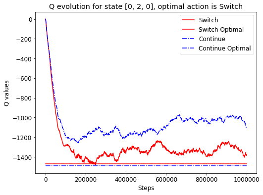
Figure 7: Although the agent has seen state (0,2,0) frequently, it learns the nonoptimal action ranking.

We now examine in more detail why the $Q$ values are not converging to the optimal values. As discussed in Section 3, the $Q$ value updates are driven by the realized TD-errors. (Note that although the expected TD-errors are $0$ in the optimal solution, the realized TD-errors for individual samples from the replay buffer may not be $0$, even at optimality.) We follow the outline of [1] and measure the updates to a $Q$ value according to whether we train on the corresponding state/action pair or not.

Figure 8 shows the evolution of the TD-error over all state/action pairs that we train on. The color of the point represents the frequency with which the associated state is visited. We note that the TD-error is smaller for the states that are visited frequently compared to the states that are visited less often. This matches the intuition captured in Section 3 that we have smaller error for $Q$ values whose update is due to training on the corresponding state, compared to $Q$ values that we rarely train on directly but whose updates are due to the generalization of the NN. For this latter class of states, we observe that the TD-error increases over time. (We remark that the outliers at the bottom of the plot are artifacts of how Stable Baselines computes TD-error whenever we reset to the initial state (which we do every 1000 steps.))

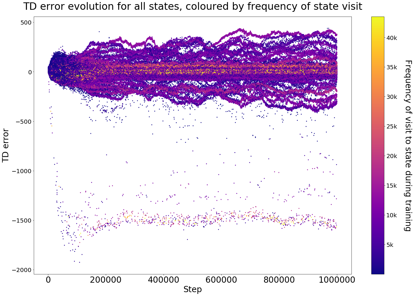
Figure 8: The evolution of the TD-error values.

In Figure 9 we restrict our attention to just 3 state/action pairs: $((1,5,0),\mbox{\em switch})$ that is visited with high frequency, $((0,2,0),\mbox{\em continue})$ that is visited with medium frequency, and $((0,5,1),\mbox{\em switch})$ that is visited with low frequency. The high frequency and low frequency states have TD-errors that are clustered around zero. However, state $((0,2,0),\mbox{\em continue})$ has two distinct bands. We now investigate why that occurs.

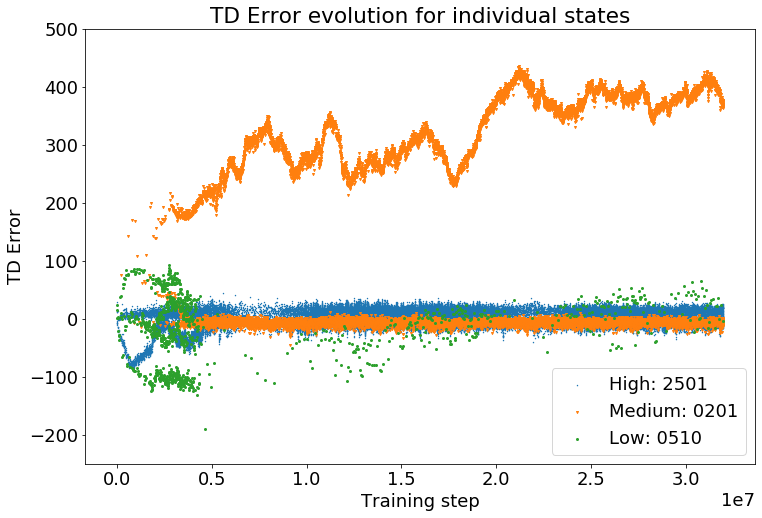
Figure 9: TD-errors for 3 states. The plot has been clipped to exclude outliers and sampled down for legibility.

First, note that the continue action consistently has the higher $Q$ value in Figure 7. Hence this is the action that is taken in this state (unless there is an exploration step). The value of the TD-error for $((0,2,0),\mbox{\em continue})$ depends on the arrivals into the queues. If the next state is $(0,2,0)$ or $(1,2,0)$ then we observe that the TD-error is small and negative, around $-10.3\pm 4.7$. However, if the next state is $(0,3,0)$ or $(1,3,0)$ then the TD-error is large and positive, around $299.335\pm 4.188$.

Motivated by the discussion in Section 3, we consider two situations according to whether we train on the state/action pair, $((0,2,0),\mbox{\em continue})$. If we do train on that pair, then we distinguish based on the sign of the TD-error. Hence, we consider the following cases:

• Case 1a. The state/action pair $((0,2,0),\mbox{\em continue})$ is in the sampled batch with a small negative TD-error.

• Case 1b. The state/action pair $((0,2,0),\mbox{\em continue})$ is in the sampled batch with a large positive TD-error.

• Case 2. The state/action pair $((0,2,0),\mbox{\em continue})$ is not in the sampled batch.

If the NTK were close to the identity matrix then we would expect the $Q$ value for $((0,2,0),\mbox{\em continue})$ to go up by a small amount in Case 1a and go down by a large amount in Case 2b. However, the NTK will typically have off-diagonal terms in order to produce the generalization across multiple states. In particular, the $Q$ value for $((0,2,0),\mbox{\em continue})$ will typically change even if that state/action pair is not in the sampled batch.

Figure 10 shows the change in $Q$ value for $((0,2,0),\mbox{\em continue})$ in Case 1a (red), Case 1b (green) and Case 2 (blue) during steps 499,500 to 499,700. The horizontal lines show the average change for each case. Although the NN-based function approximation causes these changes to be noisy, the $Q$ values do move in the correct direction. In particular,

• The average change in $Q$ value for Case 1a is $0.0711$.

• The average change in $Q$ value for Case 1b is $-0.0980$.

• The average change in $Q$ value for Case 2 is $-0.0003$.

However, the reason that the $Q$ value does not make progress towards the optimal value is that there is no discernible difference in the magnitude of the change in $Q$ value in the case that the TD-error has large magnitude (and positive sign) versus the case that the TD-error has small magnitude (and negative sign). We see this behavior throughout our runs and view this as the main reason why the $Q$ values do not converge to optimal.

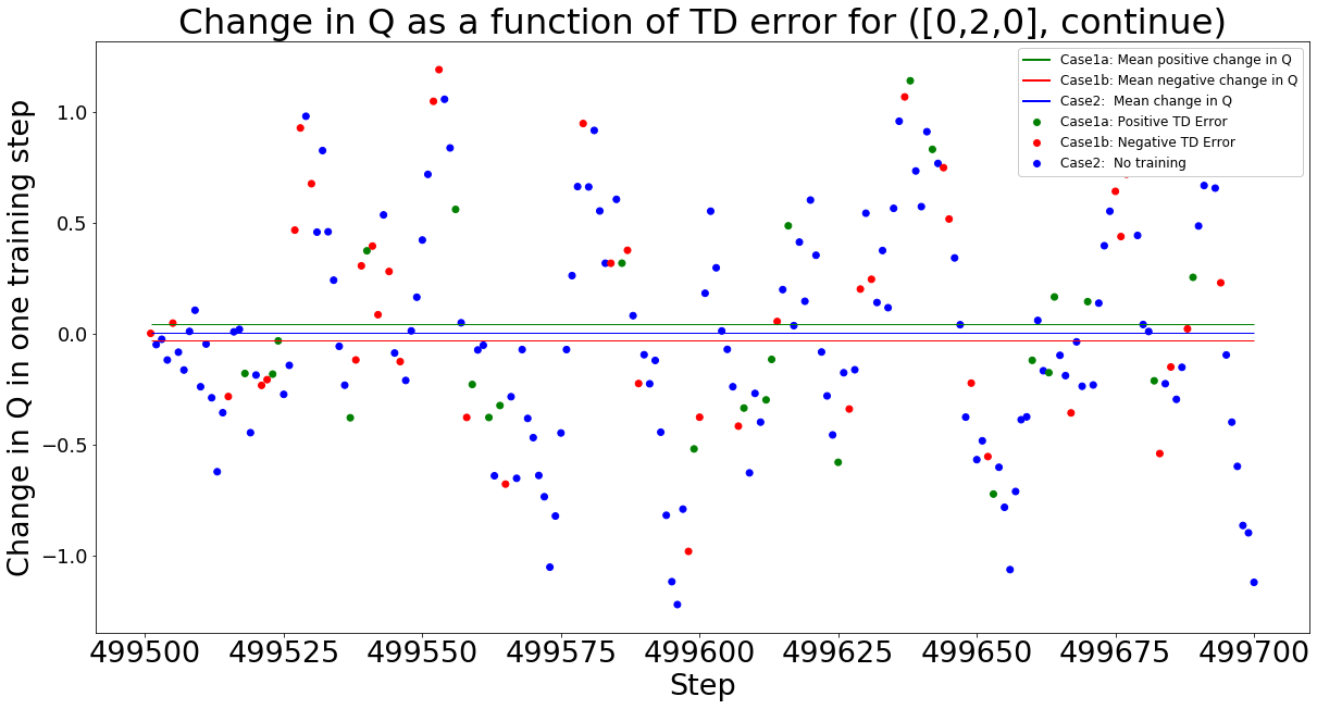
Figure 10: Change in $Q$ value for $((0,2,0),\mbox{\em continue})$ for a small sample of steps. Red - Case 1a, Green - Case 1b, Blue - Case 2.

5 Conclusions

In this paper we have shown that even for the start-of-the-art implementation of DQL in Stable Baselines, there are simple environments where the $Q$ values do not reach the optimal point. If different actions in the same state have similar optimal $Q$ values then this can lead to incorrect decisions. We explain this behavior by examining the $Q$ value update produced by the neural network as a function of the TD-error. In particular, large TD-errors do not necessarily produce a large change in $Q$ value (which would occur with regular $Q$ learning). In future work we plan to expand the taxonomy of environments for which DQL has difficulty reaching the correct values.

References

- [1] J. Achiam, E. Knight, and P. Abbeel. Towards characterizing divergence in deep Q-learning. CoRR, abs/1903.08894, 2019.
- [2] D. Silver, T. Hubert, J. Schrittwieser, I. Antonoglou, M. Lai, A. Guez, M. Lanctot, L. Sifre, D. Kumaran, T. Graepel, T. Lillicrap, K. Simonyan, and D. Hassabis. Mastering chess and shogi by self-play with a general reinforcement learning algorithm. CoRR, abs/1712.01815, 2017.
- [3] S. Arora, R. Ge, B. Neyshabur, and Y. Zhang. Stronger generalization bounds for deep nets via a compression approach. In Proceedings of the 35th International Conference on Machine Learning, ICML 2018, Stockholmsmässan, Stockholm, Sweden, July 10-15, 2018, pages 254–263, 2018.
- [4] A. Hill, A. Raffin, M. Ernestus, A. Gleave, A. Kanervisto, R. Traore, P. Dhariwal, C. Hesse, O. Klimov, A. Nichol, M. Plappert, A. Radford, J. Schulman, S. Sidor, and Y. Wu. Stable baselines. https://github.com/hill-a/stable-baselines, 2018.
- [5] S. Sidor and J. Schulman. OpenAI baselines. https://blog.openai.com/openai-baselines-dqn/, 2017.
- [6] T. Simonini. On choosing a deep reinforcement learning library. https://medium.com/data-from-the-trenches/, 2019.
- [7] V. Mnih, K. Kavukcuoglu, D. Silver, A. Graves, I. Antonoglou, D. Wierstra, and M. Riedmiller. Playing Atari with deep reinforcement learning. CoRR, abs/1312.5602, 2013.
- [8] C. Watkins and P. Dayan. Technical note Q-learning. Machine Learning, 8:279–292, 1992.
- [9] G. Brockman, V. Cheung, L. Pettersson, J. Schneider, J. Schulman, J. Tang, and W. Zaremba. OpenAI gym. CoRR, abs/1606.01540, 2016.
- [10] H. Wei, G. Zheng, H. Yao, and Z. Li. Intellilight: A reinforcement learning approach for intelligent traffic light control. In Proceedings of the 24th ACM SIGKDD International Conference on Knowledge Discovery & Data Mining, KDD 2018, London, UK, August 19-23, 2018, pages 2496–2505, 2018.
- [11] Z. Wang, T. Schaul, M. Hessel, H. van Hasselt, M. Lanctot, and N. de Freitas. Dueling network architectures for deep reinforcement learning. In Proceedings of the 33nd International Conference on Machine Learning, ICML 2016, New York City, NY, USA, June 19-24, 2016, pages 1995–2003, 2016.
- [12] V. François-Lavet, P. Henderson, R. Islam, M. Bellemare, and J. Pineau. An introduction to deep reinforcement learning. CoRR, abs/1811.12560, 2018.
- [13] Z. Yang, Y. Xie, and Z. Wang. A theoretical analysis of deep Q-learning. CoRR, abs/1901.00137, 2019.
- [14] S. Fujimoto, H. van Hoof, and D. Meger. Addressing function approximation error in actor-critic methods. In Proceedings of the 35th International Conference on Machine Learning, ICML 2018, Stockholmsmässan, Stockholm, Sweden, July 10-15, 2018, pages 1582–1591, 2018.
- [15] J. Fu, A. Kumar, M. Soh, and S. Levine. Diagnosing bottlenecks in deep Q-learning algorithms. In Proceedings of the 36th International Conference on Machine Learning, ICML 2019, 9-15 June 2019, Long Beach, California, USA, pages 2021–2030, 2019.
- [16] H. van Hasselt, Y. Doron, F. Strub, M. Hessel, N. Sonnerat, and J. Modayil. Deep reinforcement learning and the deadly triad. CoRR, abs/1812.02648, 2018.
- [17] Z. Lipton, J. Gao, L. Li, J. Chen, and L. Deng. Combating reinforcement learning’s sisyphean curse with intrinsic fear. CoRR, abs/1611.01211, 2016.
- [18] O. Anschel, N. Baram, and N. Shimkin. Averaged-DQN: Variance reduction and stabilization for deep reinforcement learning. In Proceedings of the 34th International Conference on Machine Learning, ICML 2017, Sydney, NSW, Australia, 6-11 August 2017, pages 176–185, 2017.
- [19] T. Lu, D. Schuurmans, and C. Boutilier. Non-delusional Q-learning and value-iteration. In Advances in Neural Information Processing Systems 31: Annual Conference on Neural Information Processing Systems 2018, NeurIPS 2018, 3-8 December 2018, Montréal, Canada, pages 9971–9981, 2018.
- [20] Arthur Jacot, Franck Gabriel, and Clément Hongler. Neural tangent kernel: Convergence and generalization in neural networks. CoRR, abs/1806.07572, 2018.