Shortcomings of transfer entropy and partial transfer entropy: Extending them to escape the curse of dimensionality

Abstract

Transfer entropy (TE) captures the directed relationships between two variables. Partial transfer entropy (PTE) accounts for the presence of all confounding variables of a multivariate system and infers only about direct causality. However, the computation of PTE involves high dimensional distributions and thus may not be robust in case of many variables. In this work, different variants of PTE are introduced, by building a reduced number of confounding variables based on different scenarios in terms of their interrelationships with the driving or response variable. Connectivity-based PTE variants and utilizing the random forests (RF) methodology are evaluated on synthetic time series. The empirical findings indicate the superiority of the suggested variants over TE and PTE, especially in case of high dimensional systems.

Keywords Granger causality  $\cdot$ multivariate time series  $\cdot$ curse of dimensionality  $\cdot$ partial transfer entropy  $\cdot$ variable selection  $\cdot$ random forests

1 Introduction

Connectivity analysis deals with the interdependence relationships between two or more variables. There are two distinct cases of interdependence. In the first case, the variables evolve in synchrony and we are interested in correlations. Correlation measures express the empirical association between variables while quantifying their dependence. In the second one, a variable drives another one and they are connected with a causal relationship.

The investigation of the dynamical causal relationships between the variables of a multivariate system is essential in a variety of applications, such as physiology, e.g. to understand the links between functional cerebral functions and their underlying brain mechanisms [1, 2, 3], and finance, e.g. to determine the possible sources of inflation and therefore decide on policies to reduce it [4, 5].

Since the pioneering work by Granger [6], the advance on Granger causality (GC) has grown considerably. Transfer entropy (TE) is its information-theoretic analog [7, 8], relying on the same idea, i.e.  if the prediction of a time series could be improved by incorporating the knowledge of past information of another one, then the latter is considered to have a causal influence on the former. Unlike the standard GC test, the TE does not rely on any model or assumption on the nature of the data, while identifies both linear and nonlinear interrelationships. TE has proved to be effective in a variety of simulation studies and real applications [9, 10, 11, 12, 13]. For a review on TE, see [14].

Bivariate approaches, such as GC and TE, may suffer from shortcomings, such as omitted variable bias [15] and thereby can lead to erroneous conclusions. The importance of using multivariate methods has been emphasized in a variety of works, such as in [16, 17, 18], since they provide a better representation of real-world interactions. Direct causality measures and tests exploit all the available information from the whole set of the observed variables of a multivariate system and indicate only the direct causality between variables, excluding indirect causality from intermediate variables, such as the causality $X\rightarrow Y$ stemming from the intermediate variable $Z$: $X\rightarrow Z\rightarrow Y$.

The GC has been extended in the multivariate case in order to infer only direct causality [19]. In [20], the reliability of conditional GC (CGC) is investigated in the time domain, suggesting that a large number of time points decreases the reliability of the results and increases the number of type I errors. A high sensitivity is established, when the underlying structure of the examined system has the delays between the interacting nodes much larger than the frequency resolution, the connection strength is higher than a specific percentage of the amplitude of the driver signal and the signal to noise ratio is not very high. Finally, indirect links were revealed by the analysis for specific connection strengths and lags. The TE has also been extended in the multivariate case, namely the Partial TE (PTE), while different estimators of PTE have been proposed, such as based on binning [21], correlation sums [22] and $k$-nearest neighbors (KNN) [23]. The PTE though seems to be only effective for low dimensional systems [22, 24, 23, 25].

A non-uniform embedding scheme (NUE) for the estimation of a direct coupling information measure has been suggested in [26]. However, as the dimensionality of a system increases, even the most effective measures utilizing dimension reduction techniques, may fail. That is because the curse of dimensionality re-emerges at some point when original data are of high dimensionality since the majority of the proposed dimension reduction methods proceed by estimating probability distributions of increasing dimensions.

Further extending CGC and taking into consideration the above computational limitations, the partially conditioned GC (PCGC) is introduced [27]. In this work, a subset of conditioning variables is used for the estimation of multivariate GC based on a mutual information criteria. The PCGC is shown to significantly improve the performance of standard linear GC. As stated in [27]: "conditioning on a small number of variables, chosen as the most informative ones for the driver node, leads to results very close to those obtained with a fully multivariate analysis and even better in the presence of a small number of samples."

In view of all the above, we suggest an ensemble of different variations of the original PTE, aiming to improve the performance of PTE for high dimensional data by reducing the number of the conditioning variables. The PTE variants can be easily implemented and are feasible on arbitrary data dimension. To formulate the PTE variants, the connectivity relationships between the driving or response variable to the confounding ones is examined, while also a more sophisticated method is utilized for variable selection, namely the random forests (RF) method [28]. The proposed PTE variants are compared to each other, to the bivariate TE and the multivariate PTE on known simulation systems. Results suggest that when dimensionality increases, the PTE variants outperform both TE and PTE. Through the simulation study, the advantages and shortcomings of TE and PTE are displayed in detail.

The rest of the paper is organized as follows. In Section 2, the PTE variants are introduced. In Section 3, the performance of the PTE variants is displayed based on Monte Carlo simulations on known coupled systems and compared with TE and PTE. Finally, Section 4 concludes.

2 Methods

In this section, we briefly review the causality measures transfer entropy (TE) and partial transfer entropy (PTE), illustrate the significance test for the non-causality hypothesis and finally introduce the ensemble of PTE variants.

2.1 Transfer Entropy

The transfer entropy (TE) is a nonlinear measure that quantifies the amount of information explained in $Y$ at $h$ time steps ahead from the state of $X$ accounting for the concurrent state of $Y$ [29]. Let ${x_{t}}$, ${y_{t}}$ be two stationary time series and $\textbf{x}_{t}=[x_{t},x_{t-1},\ldots,x_{(m-1)\tau}]^{\prime}$ and $\textbf{y}_{t}=[y_{t},y_{t-1},\ldots,y_{(m-1)\tau}]^{\prime}$ the reconstructed vectors of the state space of each system, where $\tau$ is the delay time and $m$ is the embedding dimension. The TE from $X$ to $Y$ can be defined based on entropy terms as

$$\mbox{TE}_{X\rightarrow Y}=-H(y_{t+h}|\textbf{x}_{t},\textbf{y}_{t})+H(y_{t+h}|\textbf{y}_{t})$$ (1)

where $H(x)$ is the Shannon entropy of the variable $X$.

2.2 Partial Transfer Entropy

The partial transfer entropy (PTE) is the extension of the TE accounting for the direct causal effect of $X$ to $Y$ conditioning on all the remaining variables of a multivariate system, let us denote them $Z=Z_{1},\ldots,Z_{K-2}$ (confounding variables). Let us denote by $\textbf{z}_{t}$ the reconstructed vectors of all the variables in $Z$. The direct causal effect of $X$ to $Y$ measured by PTE is expressed as

$$\mbox{PTE}_{X\rightarrow Y|Z}=-H(y_{t+h}|\textbf{x}_{t},\textbf{y}_{t},\textbf{z}_{t})+H(y_{t+h}|\textbf{y}_{t},\textbf{z}_{t})$$ (2)

The entropy terms of TE and PTE are estimated here using the $k$-nearest neighbors (KNN) method [30, 23], which is stable, not significantly affected by the choice of $k$ [30] and gives better estimates at moderate dimensions compared to other estimators [23].

2.3 Statistical Significance

In order to decide whether a small positive value of TE / PTE is significant or not, resampling methods are required. To assess the statistical significance of the TE / PTE, the empirical null distribution is constructed based on resampled time series. For this, $100$ time-shifted surrogates [31] are constructed, randomizing only the driving time series, while the significance level is $\alpha=0.05$. If the estimated value of the causality measure from the original time series is at the tail of the null distribution formed by the surrogates, then the null hypothesis H₀ of non-causality is rejected. The $p$-value of the one-sided test is computed by applying the correction for the empirical cumulative density function as given in [32].

2.4 PTE variants

Let us suppose there is a multivariate system in $K$ variables. The estimation of any direct causality measures for a pair of observed variables (e.g. for $X\rightarrow Y$) involves also the remaining $K-2$ observed variables (e.g. $Z=Z_{1},\ldots,Z_{K-2}$). Since the computation also includes the lagged variables in past times, the corresponding dimensionality increases even more.

We note that the following estimation scenarios can be implemented on any multivariate causality measure, however we will focus only on PTE since the comparisons of the different scenarios must be conducted with respect to a specific causality measure.

First, we introduce an ensemble of connectivity-based PTE variants. They are formed so that the original number of conditional variables ($K-2$) is reduced. We set the number of conditioning variables equal to a fixed number $nc$; the optimal choice of $nc$ is also investigated. First, the criteria for forming the subset of conditioning variables relies on a connectivity measure. Specifically, the linear correlation coefficient (CC), $r=cov(X,Y)$ / $(\sigma_{X}\sigma_{Y})$, and the mutual information (MI), a general measure of mutual dependence between two variables from information theory, defined on entropy terms as $I=I(X,Y)=H(X)-H(X|Y)$ are considered.

Regarding the connectivity-based variants, if the subset of conditioning variables satisfying each corresponding criterion is smaller than the desired one, then this reduced number of conditioning variables is utilized. If none of the confounding variables satisfy the corresponding criterion, then the bivariate TE is estimated instead. The statistical significance of $r$ is assessed on the statistic $t=r\sqrt{\frac{n-2}{1-r^{2}}}$, which follows the $t$-distribution with $n-2$ degrees of freedom. On the other hand, the significance of MI is assessed non-parametrically, by randomly permuting one of the two involved time series and the $p$-values are estimated from the one sided-test for the null that the two variables are independent.

As an alternative, we exploit the random forests (RF) methodology [33, 34], in order to determine the most ’important’ determinants for a specific target variable. RF is a sophisticated method, introduced for handling big data, such as for hundreds or even millions of observations [35]. It is a machine learning method based on decision trees. It is a form of nonlinear regression model where samples are partitioned at each node of a binary tree based on the value of one selected input feature. The input of each tree is sampled data from the original dataset. A subset of features is randomly selected from the optional features to grow the tree at each node. Each tree is grown without pruning. In this work, the implementation of RF for variable selection relies on the tree minimal depth methodology [36], a method that determines the variable importance by the position of the variables in the decision trees and thus is only based on the decision tree structures. In this case, $nc$ is automatically specified by the RF method and not a’ priori selected as in case of the connectivity-based variants.

The ensemble of the proposed connectivity-based (1A - 4B) and RF-based (5A - 5C) variants of PTE consider different subsets of conditioning variables selected from the original set of confounding variables. Specifically, the subset of the conditioning variables is defined by the following criteria:
1A: Choose the most correlated variables to the driving one based on $r$
1B: Choose the most correlated variables to the driving one based on $I$
2A: Choose the least associated variables to the driving one based on $r$
2B: Choose the least associated variables to the driving one based on $I$
3A: Choose the most correlated variables to the response one based on $r$
3B: Choose the most correlated variables to the response one based on $I$
4A: Choose the least associated variables to the response one based on $r$
4B: Choose the least associated variables to the response one based on $I$.
5A: Choose the most associated variables to the driving one based on RF
5B: Choose the most associated variables to the response one based on RF
5C: Choose the most associated variables to the driving and response variable based on RF

3 Numerical studies

The performance of the PTE variants is examined through simulation experiments. Three known coupled systems are considered including linear and nonlinear couplings. For comparison reasons, we also estimate the bivariate transfer entropy (TE) and the original multivariate transfer entropy (PTE), while the connectivity-based PTE variants are estimated by varying the number of the conditioning variables.

We formulate 100 realizations from each simulation system, with time series lengths $n=512,1024,2048$ and estimate the causality measures for all directions. The TE, PTE and PTE variants are computed for $h=1$ and $\tau=1$ (as in definition of TE [29]) and the embedding dimension $m$ is fixed based on the equations of the system. Finally, the number of neighbors for the KNN method is equal to $k=10$ ($k$ does not affect the performance of the KNN estimator [37]).

The performance of the measures is evaluated in terms of binary classification tests, where ’positive’ corresponds to the case of causality and ’negative’ to the non-causal case. Specifically, results are discussed by considering three classification measures; sensitivity, specificity and F1-score. First, we estimate the number of ’positives’ and ’negatives’ found, where: True Positive (TP) stands for causal link correctly classified as positive, True Negative (TN) for a non-causal links correctly classified as negatives, False Positive (FP) for non-causal inks erroneously classified as positive, and False Negative (FN) for a causal link erroneously classified as negatives. The sensitivity (Sen) or true positive rate measures the proportion of actual positives that are correctly identified as such by the measure, i.e. we evaluate the ability of the measures to detect the true causal effects:

$$Sensitivity=TP/(TP+FN)$$

The specificity (spec) or true negative rate quantifies the proportion of actual negatives that are correctly identified as such, i.e. indicates the ability of a measure to correctly detect the non-causal variables:

$$Specificity=TN/(TN+FP)$$

In theory, sensitivity and specificity are independent in the sense that it is possible that they both achieve their best value ($100\%$). Finally, the F1-score determines the overall test’s accuracy:

$$F1-score=2TP/(2TP+FP+FN).$$

3.1 (S1) Simulation system 1

The first simulation system is a VAR(4) process in five variables with $X_{1}\rightarrow X_{2}$, $X_{1}\rightarrow X_{4}$, $X_{2}\rightarrow X_{4}$, $X_{4}\rightarrow X_{5}$, $X_{5}\rightarrow X_{1}$, $X_{5}\rightarrow X_{2}$ and $X_{5}\rightarrow X_{3}$ [38]

$$x_{1,t} = 0.4x_{1,t-1}-0.5x_{1,t-2}+0.4x_{5,t-1}+\epsilon_{1,t}$$

$$x_{2,t} = 0.4x_{2,t-1}-0.3x_{1,t-4}+0.4x_{5,t-2}+\epsilon_{2,t}$$

$$x_{3,t} = 0.5x_{3,t-1}-0.7x_{3,t-2}-0.3x_{5,t-3}+\epsilon_{3,t}$$

$$x_{4,t} = 0.8x_{4,t-3}+0.4x_{1,t-2}+0.3x_{2,t-3}+\epsilon_{4,t}$$

$$x_{5,t} = 0.7x_{5,t-1}-0.5x_{5,t-2}-0.4x_{4,t-1}+\epsilon_{5,t},$$

where $\epsilon_{i,t}$, $i=1,\ldots,5$ are independent to each other Gaussian white noise processes with unit standard deviation.

Causality measures are estimated for $m=4$ (the maximum delay in the system’s equations). First, results for TE and PTE are reported in Table 1. Sensitivity (Sen), specificity (Spec) and F1-score are computed from 100 realization of the system for each time series length $n$ and finally as a mean over all $n$. Bivariate TE has a higher sensitivity compared to PTE, while multivariate PTE outperforms TE regarding specificity. In particular, TE has a high sensitivity which increases with $n$, but has a relatively low specificity that decreases as $n$ gets larger. On the other hand, PTE may has a slightly lower sensitivity compared to TE, but it increases with $n$. Additionally, specificity for PTE decreases with $n$. Overall, the PTE ($88.24\%$) outstands TE ($75.45\%$), based on the mean F1-score over all $n$.

Table 1: Classification measures for TE and PTE for S1, as a mean over all realizations for each time length $n$.

	TE			PTE
	Sen	Spec	F1-score	Sen	Spec	F1-score
$n=512$	98.43	75	80.89	79.86	92.92	82.72
$n=1024$	99.86	64.69	75.58	93.71	92.77	90.72
$n=2048$	100	53.15	69.87	98.29	90.38	91.27
MEAN	99.43	64.28	75.45	90.62	92.03	88.24

In order to further analyze the above quantitative results, the significant causal effects over all realizations are examined for all couples of variables. As expected, TE indicates both direct and indirect causal effects. As $n$ increases, the percentages of significant indirect causalities also increase, leading to a decreasing specificity and thus a decreasing overall performance (F1-score). Since PTE is multivariate, is expected to only indicate direct couplings, while for $K=5$, no major estimation problems should arise due to high dimensionality. For small $n$, the percentages of significant causality are low only for $X_{2}\rightarrow X_{4}$ ($28\%$ for $n=512$, $68\%$ for $n=1024$, $88\%$ for $n=2048$) and $X_{5}\rightarrow X_{3}$ ($64\%$ for $n=512$, $89\%$ for $n=1024$, $100\%$ for $n=2048$), while the indirect coupling $X_{5}\rightarrow X_{4}$ is obtained ($24\%$ for $n=512$, $31\%$ for $n=1024$, $50\%$ for $n=2048$). The above findings can be summarized in Fig. 1, where the true network and the corresponding detected networks by TE and PTE are presented.

Figure 1: The true network of S1 in (a) and the extracted networks based on TE in (b) and on PTE in (c). Dashed lines indicate indirect causalities.

The PTE variants that rely on the connectivity criteria are estimated by setting the number of conditioning variables equal to $nc=1$ and $nc=2$. Empirical findings from S1 show that CC gives many significant linear correlations which increase with $n$. On the other hand, MI detects much fewer correlations compared to linear CC. All the PTE variants have slightly higher sensitivity compared to PTE but lower compared to TE (Table 2). Further, they present higher specificity compared to TE but lower specificity compared to PTE. As $n$ increases, the sensitivity of the variants slightly increases while the specificity decreases. Their overall performance worsens since specificity mostly affects it.

Table 2: Classification measures for connectivity-based PTE variants for S1, as a mean over all realizations for each time length $n$ and number of conditioning variables $nc$.

	$nc=1$
	$n=512$			$n=1024$			$n=2048$
	Sen	Spec	F1-score	Sen	Spec	F1-score	Sen	Spec	F1-score
1A	92.57	85.85	84.78	98.86	80.23	84.45	100	73.38	80.55
1B	94.43	81.61	82.97	99.29	75	81.32	100	67.62	77.31
2A	91.86	84.92	83.99	96.86	80.23	83.41	99.86	70.23	78.83
2B	91	85.62	83.96	96.29	78.15	81.91	99.71	70.92	79.12
3A	93	85.54	84.88	97.71	78.77	82.79	99.86	72.38	79.98
3B	95.14	79.31	81.95	98.71	72.62	79.46	100	67.46	77.21
4A	90.14	85.54	74.29	96.14	79.92	82.75	99.86	64	75.4
4B	90.71	85.31	83.74	97.43	78	82.26	99.57	70.92	78.97
	$nc=2$
1A	90.14	85.77	83.45	95.86	83.23	84.86	98.71	76.92	82.2
1B	94	81.85	82.9	99.29	75.85	81.84	99.71	69.46	78.18
2A	88.43	87.85	84.03	96.14	83.85	85.42	99.86	70.23	78.83
2B	85.71	88.92	83.32	95.57	85.77	86.4	99	80.38	84.51
3A	91.43	86.85	84.92	96.43	83.92	85.7	99.86	81.92	86.09
3B	95	79.46	81.95	98.43	73.23	79.72	100	68.46	77.78
4A	87.14	88	83.53	96.29	80.23	83.04	99.57	64.38	75.48
4B	85.57	90.38	84.19	86.77	86.77	86.86	98.14	81	84.62

The number of conditioning variables also influences the performance of the connectivity-based variants. For $nc=1$, we have always slightly higher sensitivity compared to $nc=2$. On the contrary, for $nc=2$, we have always slightly higher specificity compared to $nc=1$. The best performance among the PTE variants is obtained for variant 3A, i.e. when choosing the conditioning variables as the most correlated to the response one. The mean F1-score over all realizations and time series lengths for 3A is $85.57\%$, very close to PTE’s mean performance ($88.24\%$), but much higher than TE’s ($75.45\%$).

Regarding the RF-based variants, 5C coincides with the multivariate case, i.e. coincides with PTE, thus scoring the highest F1-score. The variant 5A slightly outperforms all the considered connectivity-based variants, achieving a mean F1-score equal to $86.58\%$ and 5B follows, scoring very closely (mean F1-score $86.44\%$) (Table 3).

Table 3: Classification measures for RF-based PTE variants for S1, as a mean over all realizations for each time length $n$.

	$n=512$			$n=1024$			$n=2048$
	Sen	Spec	F1-score	Sen	Spec	F1-score	Sen	Spec	F1-score
5A	91.71	85.23	83.93	95	87.15	87.12	98.71	86.31	88.69
5B	91.57	83.85	82.97	95.14	87.69	87.63	98.57	86.5	88.72

3.2 (S2) Simulation system 2

We consider a system with linear ($X_{1}\rightarrow X_{3}$, $X_{4}\leftrightarrow X_{5}$) and nonlinear couplings ($X_{1}\rightarrow X_{2}$, $X_{1}\rightarrow X_{4}$) given by the equations:

$$x_{1,t} = 0.95\sqrt{2}x_{1,t-1}-0.9025x_{1,t-2}+\epsilon_{1,t}$$

$$x_{2,t} = 0.5x_{1,t-2}^{2}+\epsilon_{2,t}$$

$$x_{3,t} = -0.4x_{1,t-3}+\epsilon_{3,t}$$

$$x_{4,t} = -0.5x_{1,t-2}^{2}+0.25\sqrt{2}x_{4,t-1}+0.25\sqrt{2}x_{5,t-1}+\epsilon_{4,t},$$

$$x_{5,t} = -0.25\sqrt{2}x_{4,t-1}+0.25\sqrt{2}x_{5,t-1}+\epsilon_{5,t},$$

with Gaussian noise terms as in S1 [18].

The TE indicates correctly the true causality. However, it also detects the indirect causal link $X_{1}\rightarrow X_{5}$, e.g. for $n=2048$, with percentage $100\%$. Additionally, the spurious links $X_{2}\rightarrow X_{3}$ ($100\%$), $X_{2}\rightarrow X_{4}$ ($100\%$), $X_{2}\rightarrow X_{5}$ ($100\%$), $X_{3}\rightarrow X_{2}$ ($80\%$), $X_{3}\rightarrow X_{4}$ ($78\%$), $X_{3}\rightarrow X_{5}$ ($100\%$), $X_{4}\rightarrow X_{2}$ ($100\%$), $X_{4}\rightarrow X_{3}$ ($100\%$), $X_{5}\rightarrow X_{2}$ ($100\%$), $X_{5}\rightarrow X_{3}$ ($100\%$) are obtained (percentages are indicatively shown for $n=2048$).

The PTE indicates almost all the true links; it fails to identify the true relationship $X_{5}\rightarrow X_{4}$. Further, it indicates the indirect effect $X_{1}\rightarrow X_{5}$ ($100\%$ for $n=2048$) and the false ones $X_{2}\rightarrow X_{4}$ ($100\%$), $X_{2}\rightarrow X_{5}$ ($100\%$), $X_{3}\rightarrow X_{5}$ ($21\%$), $X_{5}\rightarrow X_{2}$ ($18\%$).

The extracted outcomes of the binary classification measures regarding TE and PTE are displayed on Table 4. The overall performance of TE is low. TE has a high sensitivity that sligthly increases with $n$, however obtains a very low specificity which decreases with $n$. On the other hand, PTE has lower sensitivity compared to TE but still on a high level. It also achieves a high specificity. Both the sensitivity and specificity of PTE decrease with $n$. The mean F1-score of TE and PTE over all $n$ is $39.12\%$ and $65.7\%$, respectively. Overally, the PTE outperforms the TE, however cannot succeed a high mean F1-score.

Table 4: Classification measures for TE and PTE for S2, as a mean over all realizations for each $n$.

	TE			PTE
	Sen	Spec	F1-score	Sen	Spec	F1-score
$n=512$	89.80	33.33	46.38	82.4	80.27	68.6
$n=1024$	93.20	29.93	46.27	81.6	76.27	64.8
$n=2048$	96.80	29.47	47.47	80.6	75.33	63.58
MEAN	93.27	30.91	39.12	81.53	78.35	65.7

For S2, the MI detects more correlations compared to the linear CC. Cumulative results over all realizations and time series lengths are presented in Table 5, for the connectivity based PTE variants. Sensitivity is high and increases with $n$ for both $nc$ (varies from $82.2\%$ to $96.4\%$), specificity is low (varies from $34.53\%$ to $72\%$) but increases with $n$. Both sensitivity and specificity are in-between the estimated corresponding values from TE and PTE. The PTE variants have slightly higher sensitivity compared to PTE ($80.60\%$) but lower compared to TE ($96.80\%$). The PTE variants have higher specificity compared to TE ($30.91\%$) but lower specificity than PTE ($75.33\%$). All variants outperform TE, however cannot reach the mean F1-score of PTE due to their low specificity. For $nc=1$, we have equal or slightly higher sensitivity compared to $nc=2$. For $nc=2$, we have always slightly higher specificity compared to $nc=1$. The best performance among PTE variants is obtained for the case 1B (mean F1-score $61.15\%$), i.e. when choosing the conditioning variables as the most correlated to the driving one using MI.

Table 5: Classification measures for connectivity-based PTE variants for S2, as a mean over all realizations and time series lengths for each $nc$.

	$nc=1$			$nc=2$
	Sen	Spec	F1-score	Sen	Spec	F1-score
1A	84.33	55.33	53.3	84.93	60.56	56.39
1B	89.93	54.76	55.51	85.73	67.91	61.15
2A	90.27	42.8	50.31	86.4	45.4	49.85
2B	92.87	38.49	49.55	92.87	39.53	50
3A	84.33	47.16	49.78	84.53	49.24	50.74
3B	84.13	48.6	50.33	83.53	49.98	50.72
4A	90.33	48.53	52.66	85.67	55.53	54.03
4B	91.07	47.71	52.61	90.73	48.58	52.89

Their poor performance is due to the detection of both indirect and spurious causalities. For case 1B, the coupling $X_{5}\rightarrow X_{4}$ is detected with a low percentage over the 100 realizations, e.g. for $n=2048$ and $nc=2$, the percentage of significant causality is $29\%$, the indirect causality $X_{1}\rightarrow X_{5}$ with $100\%$, and finally the spurious couplings $X_{2}\rightarrow X_{3}$ ($97\%$), $X_{2}\rightarrow X_{4}$ ($100\%$), $X_{2}\rightarrow X_{5}$ ($90\%$), $X_{4}\rightarrow X_{2}$ ($54\%$), $X_{3}\rightarrow X_{5}$ ($28\%$) and $X_{4}\rightarrow X_{3}$ ($26\%$) are also indicated.

Concerning the RF-based PTE variants, 5C again coincides with PTE, achieving the highest F1-score. The mean F1-score of 5A and 5B is $58.38\%$ and $50.27\%$, respectively (Table 6). Concerning S2, the connectivity-based PTE variants outstand cases 5A and 5B. Although sensitivity is high for RF-based variants, it is at a lower level compared to the connectivity-based ones. Their low specificity affects their overall performance.

Table 6: Classification measures for RF-based PTE variants for S2, as a mean over all realizations for each $n$.

	$n=512$			$n=1024$			$n=2048$
	Sen	Spec	F1-score	Sen	Spec	F1-score	Sen	Spec	F1-score
5A	87.4	64.4	59.88	87.6	62.07	58.23	85.2	61.8	57.04
5B	82.4	52.67	51.61	83	47.87	49.22	83.8	48.87	49.97

3.3 (S3) Simulation system 3

We consider a nonlinear dynamical system, the coupled Henon maps (discrete time) given by the equations:

$$x_{i,t} = 1.4-x_{i,t-1}^{2}+0.3x_{i,t-2},i=1,4$$

$$x_{i,t} = 1.4-\left(0.5c(x_{i-1,t-1}+x_{i+1,t-1})+(1-c)x_{i,t-1}\right)^{2}+0.3x_{i,t-2},i=2,\ldots,18$$

[26]. The system can be defined for an arbitrary number of variables $K$. The coupling strength is equal to $c=0.2$ (intermediate coupling strength). Estimations are displayed for the embedding dimension $m=2$ (selected based on the equations of the system).

First, we set $K=5$. For S3, MI detects only few more correlations compared to the linear CC. The binary classification measures concerning TE and PTE are presented on Table 7. Both TE and PTE correctly find the true connections of the system. The TE achieves a high sensitivity and a slightly lower specificity, resulting in a decreasing F1-score that varies from $84.7\%$ to $75.34\%$. It turns out that the decreased performance of TE is mainly due to the detection of indirect causal effects, which is expected as TE is bivariate. For example, for $n=2048$, TE indicates $X_{1}\rightarrow X_{3}$ ($64\%$), $X_{2}\rightarrow X_{4}$ ($100\%$), $X_{4}\rightarrow X_{2}$ ($100\%$), $X_{5}\rightarrow X_{3}$ ($69\%$). However, the spurious causal effect $X_{2}\rightarrow X_{1}$ ($18\%$) is also obtained. On the other hand, PTE does not indicate indirect links but falsely shows $X_{2}\rightarrow X_{1}$ ($24\%$) and $X_{4}\rightarrow X_{5}$ ($23\%$). The mean F1-score of TE and PTE over all realizations and $n$ is $80.37\%$ and $75.45\%$, respectively.

Table 7: Classification measures for TE and PTE for S3 in $K=5$ variables, as a mean over all realizations for each $n$.

	TE			PTE
	Sen	Spec	F1-score	Sen	Spec	F1-score
$n=512$	99.17	84.29	84.7	44.67	94.07	52.32
$n=1024$	100	79.36	81.07	83.17	93.03	82.79
$n=2048$	100	71.36	75.34	97.83	92.43	91.23
MEAN	99.72	78.34	80.37	75.22	93.19	75.45

The connectivity-based PTE variants have slightly lower sensitivity compared to TE but much higher compared to PTE (Table 8). Conclusively, they outperform TE and PTE. Specifically, the mean estimated F1-score over all realizations and time series for the TE is $80.37\%$, for the PTE is $75.44\%$ and for the PTE variants varies from $82.63\%$ to $89.06\%$. They have slightly lower sensitivity compared to TE but much higher compared to PTE. Their specificity is larger compared to TE but obtain lower specificity compared to PTE. For $nc=1$, we have always slightly higher sensitivity compared to $nc=2$. For $nc=2$, we have equal or slightly higher specificity compared to $nc=1$. The best performance among PTE variants is obtained for the cases 3B, i.e. when choosing the conditioning variables as the most correlated to the response one.

Table 8: Classification measures for connectivity-based PTE variants for S3 in $K=5$ variables, as a mean over all realizations and time series lengths for each $nc$.

	$nc=1$			$nc=2$
	Sen	Spec	F1-score	Sen	Spec	F1-score
1A	97.56	86.86	86.12	96.17	86.62	85.22
1B	96.89	89.07	87.65	94.83	89	86.3
2A	96.17	85.07	83.86	91.72	87.62	83.28
2B	96.33	84.17	83.32	92.78	85.95	82.63
3A	97.61	89.64	88.54	95.94	90.74	88.58
3B	97.67	90.14	89.06	95.11	91.14	88.44
4A	95.94	84.98	83.78	91.89	87.02	83.12
4B	95.94	86.07	84.57	93.33	86.14	83.14

In order to further demonstrate the performance of the optimal connectivity-based PTE variant, namely case 3B for $nc=2$, we display the estimated connectivity network from one realization of S3 (K=5,c=0.2) with $n=2048$, along with the corresponding networks for TE and PTE (Fig.  2). We further note the respective percentages of rejection of the non-causality hypothesis over the 100 realizations for each one of the detected reported causal links. All the true couplings are detected by 3B. The indirect causal links $X_{1}\rightarrow X_{3}$ ($27\%$), $X_{2}\rightarrow X_{4}$ ($14\%$), $X_{5}\rightarrow X_{3}$ ($24\%$) and the spurious links $X_{2}\rightarrow X_{1}$ ($25\%$) and $X_{3}\rightarrow X_{1}$ ($12\%$) are also obtained.

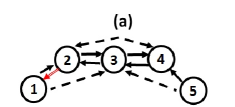
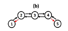
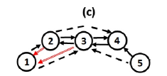
Figure 2: For S3 in $K=5$ variables ($c=0.2$), the extracted networks based on TE in (a), on PTE in (b) and on PTE variant 3B with $nc=1$ in (c). Dashed lines indicate indirect causalities. Double lines indicate spurious links.

Similarly to connectivity-based variants, the sensitivity of the RF-based variants increases with $n$, while the specificity decreases. The optimal number of conditioning variables is not significantly affected by the time series length and gets small values. The most significant variables exported from RF seem to coincide with the variables that are truly coupled, i.e. for one realization of the system, we get the following outcome: the most informative variables for variable 1 is variable 2, the most informative variables for variable 2 are variables 3 and 4, the most informative variables for variable 3 are variables 2 and 4, etc. The RF-based variant 5B, achieves the highest total mean F1-score over all realizations and time series lengths ($90.36\%$), capturing all the causal influences and slightly outperforming case 3B (Table 9). Closely scores variant 5A, with overall mean F1-score $88.67\%$, while 5C again coincides with PTE and therefore has the worst performance for S3 in $K=5$ variables.

Table 9: Classification measures for RF-based PTE variants for S3 in $K=5$ variables, as a mean over all realizations for each $n$.

	$n=512$			$n=1024$			$n=2048$
	Sen	Spec	F1-score	Sen	Spec	F1-score	Sen	Spec	F1-score
5A	92.33	92.64	88.33	99.33	90.14	86.16	100	92.64	83.68
5B	95.83	93.36	90.9	99.33	91.71	91.33	99.33	91.71	87.95

Finally, we evaluated all measures for S3 ($c=0.2$) in $K=10$ variables. Similar results are reported from S3 in $K=10$ as for $K=5$ (Table 10). The TE indicates all the true couplings and therefore has high sensitivity. But its specificity is low because many indirect causal effects and spurious ones are captured. For example, for $n=2048$, TE falsely finds the links $X_{2}\rightarrow X_{1}$ ($13\%$) and $X_{10}\rightarrow X_{9}$ ($25\%$). On the other hand, the PTE has high specificity but very low sensitivity. Although PTE also detects the true couplings, requires large time series lengths to achieve high percentages of declining the non-causal null hypothesis. Indicatively for $n=2048$, some links along with the extracted percentage over all the realizations are the following: $X_{1}\rightarrow X_{2}$ ($79\%$), $X_{2}\rightarrow X_{3}$ ($44\%$), $X_{3}\rightarrow X_{4}$ ($15\%$), $X_{4}\rightarrow X_{5}$ ($16\%$), $X_{3}\rightarrow X_{2}$ ($37\%$). The TE outperforms the PTE.

Table 10: Classification measures for TE and PTE for S3 in $K=10$ variables, as a mean over all realizations for each $n$.

	TE			PTE
	Sen	Spec	F1-score	Sen	Spec	F1-score
$n=512$	96.81	63.2	53.16	23.5	95.47	31.6
$n=1024$	99.81	52.19	40.32	28.38	94.04	35.38
$n=2048$	100	44.35	35.28	30	93.27	36.18
MEAN	98.88	53.25	48.2	27.29	94.26	34.39

Concerning the connectivity-based PTE variants, the number of conditioning variables varies from $2$ to $7$. For increasing $nc$, sensitivity decreases, while specificity increases. The best performance is for small values of $nc$. Sensitivity varies from $57.1\%$ to $88\%$ while specificity from $86.33\%$ to $93.84\%$. All the corresponding PTE variants outstand the TE (mean F1-score $48.2\%$) and the PTE (mean F1-score $36.18\%$). The optimal PTE variants are displayed in Table 11. Cases 3B and 1B for small $nc$ outperform the other cases. Thus, conditioning on the most correlated variables based on MI seems to be the best approach to improve the performance of PTE.

Table 11: Classification measures for optimal connectivity-based PTE variants for S3 in $K=10$ variables, as a mean over all realizations and time series lengths.

PTE variant	nc	Sen	Spec	F1-score
3B	2	88	90.46	76
3B	3	82.81	92.09	75.43
1B	2	78.62	93	74.61
1B	3	76.6	93.55	74.09
3B	4	76.44	92.89	72.84
1B	4	73.21	93.78	72.24
3A	3	79.42	90.37	71.04
1A	3	77	90.77	70.13

To further examine the performance of the optimal connectivity-based variant 3B, we display the extracted outcomes for all $nc$ (Table 12). As $nc$ increases, sensitivity decreases, varying from $55\%$ to $58.58\%$. Specificity achieves higher scores and has a smaller variation. It increases from $nc=2$ up to $nc=5$, where gets its highest value and then decreases again. The overall performance based on F1-score deteriorates as $nc$ grows.

Table 12: Classification measures for PTE variant 3B for S3 in $K=10$ variables, as a mean over all realizations and time series lengths.

$nc$	Sen	Spec	F1-score
2	88	90.46	76
3	82.81	92.09	75.43
4	76.44	93	74.61
5	68.77	93.55	74.09
6	62.12	92.89	72.84
7	58.58	93.78	72.24

The time series length also affects the exported results (Table 13). As $n$ gets larger, sensitivity improves, but specificity worsens. The overall performance of the measure gains strength as $n$ advances. The described course of progress regarding $nc$ and $n$ is common for all PTE variants.

Table 13: Classification measures for PTE variant 3B with $nc=2$, for S3 in $K=10$ variables, as a mean over all realizations.

$n$	Sen	Spec	F1-score
512	79.25	91.05	71.88
1024	89.44	90.43	76.79
2048	95.31	89.91	79.33
MEAN	88	90.46	76

Finally, the mean F1-score of the RF-based variants is $73.84\%$, $75.97\%$ and $46.11\%$ for 5A, 5B and 5C, respectively (Table 14). Large time series lengths are required to reach high sensitivity. Specificity is high for 5A and 5B, however both decrease with $n$. Variant 5B slightly outperforms all other cases and 5A follows closely scoring a bit lower than optimal connectivity-based variants. The poor performance of 5C is due to the increased number of conditioning variables considered. This outcome, confirms the necessity of forming a small subset of conditioning variables in order to face the curse of dimensionality.

Table 14: Classification measures for PTE variants based on RF for S3 in $K=10$ variables, as a mean over all realizations for each $n$.

	$n=512$			$n=1024$			$n=2048$
	Sen	Spec	F1-score	Sen	Spec	F1-score	Sen	Spec	F1-score
5A	68.63	93.51	69.17	79.31	92.78	74.71	84.13	92.86	77.64
5B	75.12	92.55	71.68	85.56	91.41	76.09	91.5	91.88	80.14
5C	87.25	64.49	50.01	92.19	53.74	45.6	93.5	46.91	42.71

4 Conclusion

Real world systems, such as from neuroscience and finance, usually exhibit nonlinear dynamics. Therefore, sophisticated methods are required to reveal the direction of the driving forces among the examined variables, in order to address the limitations of linear tests. Causality analysis provides a variety of methods capable of detecting directional relationships, such as transfer entropy (TE) and partial TE (PTE). This article introduces an ensemble of PTE variants, that aim to overcome the limitations of TE and PTE in case of high dimensional systems. Their advantages are highlighted mainly for high-dimensional systems, where TE and PTE perform poor.

The connectivity-based PTE variants (1A - 4B) are defined using variable selection in order to reduce the number of conditioning variables and subsequently reduce the dimensionality. The number of conditioning variables $nc$ is defined a’priori in terms of the number of the variables of the simulation system. For the PTE variants using the random forest (RF) method (5A-C), the number of conditioning variables is automatically estimated using the extracted variable importance (VIMP). The proposed PTE variants are examined in a simulation study where different types of simulation systems are considered, i.e. a linear stochastic system (S1), a stochastic system with linear and nonlinear couplings (S2) and a chaotic system with an intermediate coupling strength among the variables (S3). The systems have been selected in order to have different characteristics, i.e. unidirectional and bidirectional couplings, linear and nonlinear couplings and common drivers.

The TE, although commonly used on a variety of applications, seems to be problematic at cases. First of all, the TE is bivariate and therefore indicates both direct and indirect causal effects. However, the reduced specificity of TE in this simulation study, is only partly due to the detection of indirect causality. The inability of TE to exploit all the available information of the data, results in the identification of spurious directed links. Therefore, this is the main drawback of TE.

The PTE, is the multivariate extension of TE. By definition, it should only identify direct interrelationships. Although effective on low-dimensional systems, turns out to be problematic for high dimensional data sets. The main disadvantage of this approach is that it requires large data sets to achieve a high sensitivity. However, as the dimension of a system increases, it may not be possible to consider an adequate data size to reach a high sensitivity or to balance between sensitivity and specificity, since specificity decreases with the time series length. We should note that spurious causal influences may also appear with PTE, however seems to indicate fewer false links compared to TE in low dimensional systems.

The connectivity-based PTE variants seem to be effective, especially for high-dimensional systems. The time series length and the number of conditioning variables affects their performance, i.e. large $n$ and small $nc$ should be considered. Their performance for S1 and S2 is roughly the same, i.e. they score very close to the optimal PTE and outperform the bivariate TE. Although achieving a high sensitivity, their specificity is not that high, influencing their overall F1-score. Their effectiveness is evident in the chaotic system S3, whereas outperform TE and PTE for both $K=5$ and $K=10$, scoring much higher. Although we do not obtain the same optimal PTE variant consistently for all systems, we end up with an ensemble of conditioning variables that are mostly correlated with the driving or response variable. For S1, the optimal PTE variant is 3A; it is reasonable to come up with a case that considers the linear CC (and not MI), since S1 is linear. For S2 and S3, which are nonlinear systems, we end up with the optimal variants 1B and 3B, i.e. variants that are based on the general correlations of the examined system computed by MI.

Finally, we introduced the RF-based PTE variants. An additional advantage of these variants stands in the automatic selection of the number of conditioning variables. However, they do not have a consistent performance in the examined systems. Variants 5A and 5B score among the best measures for S1 and S3, while perform really poor for S2. Variant 5C is optimal for S1 and S2 but scores last for S3. The poor performance of 5C on high-dimensional systems is due to the fact that 5C, by construction, considers an increased number of conditioning variables compared to 5A and 5B.

To conclude, all the extracted results highlight the necessity of constructing a reduced subset of conditioning variables in order to face the curse of dimensionality when estimating multivariate causality measures. Although results are displayed for PTE, the suggested variants can be applied to any multivariate causality measure.

References

- [1] A.K. Seth, A.B. Barrett, and L. Barnett. Granger causality analysis in neuroscience and neuroimaging. Journal of Neuroscience, 35(8):3293–3297, 2015.
- [2] E. Spencer, L.-E. Martinet, E.N. Eskandar, C.J. Chu, E.D. Kolaczyk, S.S. Cash, U.T. Eden, and M.A. Kramer. A procedure to increase the power of granger-causal analysis through temporal smoothing. Journal of neuroscience methods, 308:48–61, 2018.
- [3] J. Qian, I. Diez, L. Ortiz-Terán, C. Bonadio, T. Liddell, J. Goñi, and J. Sepulcre. Positive connectivity predicts the dynamic intrinsic topology of the human brain network. Frontiers in systems neuroscience, 12:38, 2018.
- [4] G. Di Bartolomeo and E. Saltari. Current macroeconomic challenges. Macroeconomic Dynamics, 22(1):1–3, 2018.
- [5] M. Balcilar, Z.A. Ozdemir, M. Shahbaz, and S. Gunes. Does inflation cause gold market price changes? Evidence on the G7 countries from the tests of nonparametric quantile causality in mean and variance. Applied Economics, 50(17):1891–1909, 2018.
- [6] C.W.J. Granger. Investigating causal relations by econometric models and cross-spectral methods. Econometrica, 37(3):424–438, 1969.
- [7] L. Barnett, A.B. Barrett, and A.K. Seth. Granger causality and transfer entropy are equivalent for gaussian variables. Physical review letters, 103(23):238701, 2009.
- [8] K. Schindlerova. Equivalence of granger causality and transfer entropy: A generalization. Applied Mathematical Sciences, 5(73):3637–3648, 2011.
- [9] E. Siggiridou, C. Koutlis, A. Tsimpiris, V.K. Kimiskidis, and D. Kugiumtzis. Causality networks from multivariate time series and application to epilepsy. In 37th Annual International Conference of the IEEE, Engineering in Medicine and Biology Society (EMBC), pages 4041–4044, 2015.
- [10] M. Porfiri. Inferring causal relationships in zebrafish-robot interactions through transfer entropy: A small lure to catch a big fish. Animal Behavior and Cognition, 5(4):341–367, 2018.
- [11] F. Toriumi and K. Komura. Investment index construction from information propagation based on transfer entropy. Computational Economics, 51(1):159–172, 2018.
- [12] D. Gencaga. Transfer entropy. Entropy, 20(4):288, 2018.
- [13] M. Lungarella, K. Ishiguro, Y. Kuniyoshi, and N. Otsu. Methods for quantifying the causal structure of bivariate time series. International journal of bifurcation and chaos, 17(03):903–921, 2007.
- [14] T. Bossomaier, L. Barnett, M. Harré, and J.T. Lizier. An introduction to transfer entropy. Springer, 2016.
- [15] H. Lütkepohl. Non-causality due to omitted variables. Journal of Econometrics, 19(2-3):367–378, 1982.
- [16] T. Zachariadis. On the exploration of causal relationships between energy and the economy, Discussion paper 2006-05. Technical report, University of Cyprus, 2006.
- [17] K.J. Blinowska. Review of the methods of determination of directed connectivity from multichannel data. Medical & biological engineering & computing, 49(5):521–529, 2011.
- [18] A. Montalto, L. Faes, and D. Marinazzo. Mute: a matlab toolbox to compare established and novel estimators of the multivariate transfer entropy. PloS one, 9(10):e109462, 2014.
- [19] J.F. Geweke. Measures of conditional linear dependence and feedback between time series. Journal of the American Statistical Association, 79(388):907–915, 1984.
- [20] R. Franciotti and N.W. Falasca. The reliability of conditional granger causality analysis in the time domain. PeerJ Preprints, 6:e26703v1, 2018.
- [21] P.F. Verdes. Assessing causality from multivariate time series. Physical Review E, 72(2):026222, 2005.
- [22] V.A. Vakorin, O.A. Krakovska, and A.R. McIntosh. Confounding effects of indirect connections on causality estimation. Journal of neuroscience methods, 184(1):152–160, 2009.
- [23] A. Papana, D. Kugiumtzis, and P.G. Larsson. Detection of direct causal effects and application to epileptic electroencephalogram analysis. International Journal of Bifurcation and Chaos, 22(09):1250222, 2012.
- [24] D. Kugiumtzis. Partial transfer entropy on rank vectors. The European Physical Journal Special Topics, 222(2):401–420, 2013.
- [25] A. Papana, C. Kyrtsou, D. Kugiumtzis, and C. Diks. Assessment of resampling methods for causality testing: A note on the US inflation behavior. PloS one, 12(7):e0180852, 2017.
- [26] D. Kugiumtzis. Direct-coupling information measure from nonuniform embedding. Physical Review E, 87(6):062918, 2013.
- [27] D. Marinazzo, M. Pellicoro, and S. Stramaglia. Causal information approach to partial conditioning in multivariate data sets. Computational and mathematical methods in medicine, 2012:303601, 2012.
- [28] T.K. Ho. The random subspace method for constructing decision forests. IEEE Transactions on Pattern Analysis and Machine Intelligence, 20(8):832–844, 1998.
- [29] T. Schreiber. Measuring information transfer. Physical Review Letters, 85(2):461, 2000.
- [30] A. Kraskov, H. Stögbauer, and P. Grassberger. Estimating mutual information. Physical review E, 69(6):066138, 2004.
- [31] R.Q. Quiroga, A. Kraskov, T. Kreuz, and P. Grassberger. Performance of different synchronization measures in real data: A case study on electroencephalographic signals. Physical Review E, 65(4):041903, 2002.
- [32] G.-H. Yu and C.-C. Huang. A distribution free plotting position. Stochastic environmental research and risk assessment, 15(6):462–476, 2001.
- [33] T.K. Ho. Random decision forests. In Proceedings of 3rd international conference on document analysis and recognition, volume 1, pages 278–282, 1995.
- [34] L. Breiman. Random forests. Machine learning, 45(1):5–32, 2001.
- [35] R. Genuer, J.-M.l Poggi, C. Tuleau-Malot, and N. Villa-Vialaneix. Random forests for big data. Big Data Research, 9:28–46, 2017.
- [36] H. Ishwaran, U.B. Kogalur, E.Z. Gorodeski, A.J. Minn, and M.S. Lauer. High-dimensional variable selection for survival data. Journal of the American Statistical Association, 105(489):205–217, 2010.
- [37] A. Papana, C. Kyrtsou, D. Kugiumtzis, and C. Diks. Simulation study of direct causality measures in multivariate time series. Entropy, 15(7):2635–2661, 2013.
- [38] B. Schelter, M. Winterhalder, M. Eichler, M. Peifer, B. Hellwig, B. Guschlbauer, C.H. Lücking, R. Dahlhaus, and J. Timmer. Testing for directed influences among neural signals using partial directed coherence. Journal of neuroscience methods, 152(1-2):210–219, 2006.