Iterative data-driven inference of nonlinearity measures
via successive graph approximation

Abstract

In this paper, we establish an iterative data-driven approach to derive guaranteed bounds on nonlinearity measures of unknown nonlinear systems. In this context, nonlinearity measures quantify the strength of the nonlinearity of a dynamical system by the distance of its input-output behaviour to a set of linear models. First, we compute a guaranteed upper bound of these measures by given input-output samples based on a data-based non-parametric set-membership representation of the ground-truth system and local inferences of nonlinearity measures. Second, we propose an algorithm to improve this bound iteratively by further samples of the unknown input-output behaviour.

I Introduction

Deriving a controller for complex systems requires usually a sufficiently precise model. However, modelling such systems is difficult and more time consuming than the controller design. For this purpose, data-driven controller design, where a controller is obtained without identifying a model, has been investigated. [1] gives an overview of such approaches.
One data-driven approach is examined in [2] where control-theoretic system properties, as $\mathcal{L}_{2}$-gain and conic relations, are learned from given input-output samples. These properties give insight to the open-loop system and facilitate the application of well-known feedback theorems. Analogously, [3] deduces from given input-output samples a linear surrogate model that minimizes the maximal deviation to the unidentified nonlinear system. By the knowledge of the linear model and its approximation error, techniques from robust control theory can be applied to determine a controller with closed-loop guarantees. Furthermore, the approximation error corresponds to the nonlinearity measures from [4] and [5] which quantify the nonlinearity of dynamical systems.
The drawback of the approach from [2] is the requirement of a large number of input-output samples. To this end, iterative approaches are investigated where the control-theoretic properties is identified by performing sequentially experiments on the plant. These algorithms provide an (optimal) decision what experiment should be applied next to improve the estimation of the system property. For example, the $\mathcal{L}_{2}$-gain and a linear surrogate model are computed in [6] and [7], respectively, for linear time-invariant (LTI) systems based on solving optimization problems using gradient-based methods.
To deduce an iterative scheme for nonlinear systems, we exploit in this work a non-parametric data-based model. Instead of a statistical approach as in Gaussian process regression [8], we study a non-parametric set-membership model where an envelope of the graph of a Lipschitz function is described directly from given input-output data. Such Lipschitz approximations are investigated, e.g., in set-membership identification [9] and in Kinky inferences for nonlinear model predictive control [10, 11].
In this paper, we determine a guaranteed upper bound on nonlinearity measures by means of an envelope that contains the unknown input-output behaviour of the ground-truth system. Especially, the bound is obtained from the maximal distance of a linear approximation model to all realizations of mappings which are contained in the envelope. A bound on this distance is calculated by local inferences of the nonlinearity measure. Thus, this approach constitutes an alternative to [2] and [3] for deriving guaranteed bounds on system-theoretic properties from given input-output samples. Moreover, contrary to [2] and [3], the computation of the covering radius is not required and noisy output measurements can be considered. Furthermore, we extend this approach to an iterative scheme based on a branch-and-bound algorithm [12] to reduced the derived upper bound on the nonlinearity measure by further sampling. Here, we ensure that the computational complexity of this algorithm does not increase with further iterations and prove the convergence to the true nonlinearity measure in absence of noise.
In contrast to set-membership identification, we approximate the nonlinear system by a linear model that is in general not contained in the envelope. Instead, the linear model is a projection of the envelope on a set of linear models, and therefore the results of [9] are not applicable. Moreover, our goal differs from system identification in the sense that we approximate the behaviour of a complex (nonlinear) system by a simple (linear) model, i.e., the linear model is a surrogate model of the nonlinear system.
The paper is organized as follows. First, we introduce nonlinearity measures and specify the problem of estimating nonlinearity measures via graph approximation. Then we solve this problem by means of local inference of nonlinearity measures. Subsequent, we propose the iterative scheme to improve the estimation of the nonlinearity measure by successive sampling. The paper concludes with a numerical example where the iterative scheme is compared to the offline approach [3].

II Problem setup and Definition of a nonlinearity measure

Let the input-output behaviour of the unknown discrete-time nonlinear SISO system be described by the mapping

$$N:\mathcal{U}\subset\mathbb{R}^{n}\rightarrow\mathcal{Y}\subset\mathbb{R}^{n},$$

i.e. $N$ maps input on output trajectories of length $n$. We suppose that $N(0)=0$ without loss of generality.
Moreover, let the input set $\mathcal{U}$ be spanned by an orthonormal basis of signals $v_{i}\in\mathbb{R}^{n},i=1,\dots,\mu\leq n$

$$\mathcal{U}=\{u\in\mathbb{R}^{n}:u=\begin{bmatrix}v_{1}&\cdots&v_{\mu}\end{bmatrix}\bar{u},\bar{u}\in\bar{\mathcal{U}}\subset\mathbb{R}^{\mu}\}$$ (1)

where the amplitudes $\bar{u}$ are bounded by the box constraint $\bar{u}\in\bar{\mathcal{U}}=[\underline{\alpha}_{1},\bar{\alpha}_{1}]\times\dots\times[\underline{\alpha}_{\mu},\bar{\alpha}_{\mu}]$. This compact input set is also assumed in [2] and [3] since it is often considered in system identification where the basis $v_{1},\dots,v_{\mu}$ is chosen, e.g., to a Fourier basis or Legendre polynomials. Moreover, a suitable choice of basis signals ensures that all inputs which are suggested by our iterative scheme are experimentally admissible. Note that each input $u\in\mathcal{U}$ corresponds to an unique amplitude $\bar{u}\in\bar{\mathcal{U}}$ because $v_{1}\dots,v_{\mu}$ is a orthogonal basis and $\mu\leq n$. Therefore, we can exchange $u$ by its corresponding amplitude $\bar{u}$ and vice versa.
Furthermore, we suppose that $\mathcal{Y}$ is a compact set to ensure the well-definiteness of the following definition of nonlinearity measures from [4].

Definition 1 (AE-NLM).

The nonlinearity of a dynamical system $N:\mathcal{U}\subset\mathbb{R}^{n}\rightarrow\mathcal{Y}\subset\mathbb{R}^{n}$ is quantified by the additive error nonlinearity measure (AE-NLM)

$$\Phi^{\mathcal{U},\mathcal{G}}_{\text{AE}} :=\inf_{G\in\mathcal{G}}\sup_{u\in\mathcal{U}\backslash\{0\}}\frac{||N(u)-G(u)||}{||u||}$$ (2)

where $||\cdot||$ denotes the Euclidean vector norm and $G:\mathcal{U}\rightarrow\mathcal{Y}$ is an element of a set $\mathcal{G}$ of LTI systems.

Solving the optimization problem (2) yields the ‘best’ linear approximation $G^{*}$ that minimizes the gain of the error system $\Delta:=N-G^{*}$ with respect to the Euclidean norm. Thus, the nonlinear system can be written as the interconnection of the linear model $G^{*}$ and the error model $\Delta$ which gain corresponds to the AE-NLM. Therefore, techniques from robust control theory can be applied once $G^{*}$ and the nonlinearity measure are known. Furthermore, $G^{*}$ can be seen as the projection of the nonlinear system $N$ on the set of linear systems $\mathcal{G}$ as illustrated in Figure 1.

Figure 1: Projection of a nonlinear system $N$ on the set of linear models $\mathcal{G}$.

As shown in [3], the AE-NLM is related to the $\ell_{2}$-gain and the conic relations from [13] by the special choice $\mathcal{G}=\{0\}$ and $\mathcal{G}=\{G=cI:c\in\mathbb{R}\}$ with $I:u\mapsto u$, respectively. For further reading on nonlinearity measures, we refer to [3] where, amongst other things, parametrizations of $\mathcal{G}$ are proposed and a characterization of stability for feedback interconnections using nonlinearity measures is derived via the concept of graph separation.

III A data-based non-parametric model for Lipschitz mappings

In this section, we introduce the data-based non-parametric model for Lipschitz mappings from [9]. Subsequent, we specify the problem setup to calculate an upper bound for the AE-NLM from this model.
To conclude on the input-output behaviour of the unknown nonlinear system $N$, we assume the access of input-output trajectories

$$\mathcal{U}_{D}\times\mathcal{Y}_{D}:=\{(u_{1},y_{1}),\dots,(u_{D},y_{D})\}\subset\mathcal{U}\times\mathcal{Y}$$

of the nonlinear system, i.e., $y_{i}=N(u_{i}),i=1,\dots,D$. Moreover, let $\bar{\mathcal{U}}_{D}$ denote the set of amplitudes $\bar{u}_{1},\dots,\bar{u}_{D}$ that correspond to $u_{1},\dots,u_{D}$. Since the set of mappings generating $\mathcal{U}_{D}\times\mathcal{Y}_{D}$ is unbounded, the rate of variation of $N$ is restricted as in [9].

Assumption 2 (Lipschitz-continuity).

The input-output mapping $N:\mathcal{U}\rightarrow\mathcal{Y}$ is Lipschitz continuous with $L>0$, i.e.,

$$||N(u)-N(u^{\prime})||\leq L||u-u^{\prime}||,\quad\forall u,u^{\prime}\in\mathcal{U}$$

and the Lipschitz constant $L$ is known.

In general, the Lipschitz constant $L$ is not known beforehand. However, different data-driven methods were developed to estimate $L$, e.g., Strongin’s estimator [14] and POKI [15]. Under the prior knowledge of $\mathcal{U}_{D}\times\mathcal{Y}_{D}$ and Assumption 2, we can conclude that the graph of the mapping $N$ is contained in the envelope

$$E(\mathcal{U}_{D}\times\mathcal{Y}_{D}):= \{(u,y)\in\mathcal{U}\times\mathcal{Y}:||y-y_{i}||\leq L||u-u_{i}||,$$

$$\hskip 113.81102pti=1,\dots,D\}.$$

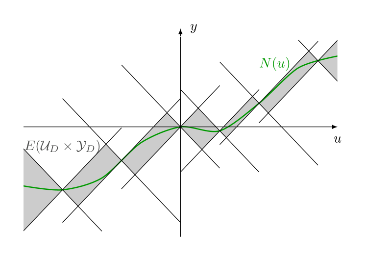
An illustration of this envelope can be found in Figure 2 for $n=1$ and in [9] for higher dimensions.

Figure 2: Envelope of an one dimensional input-output mapping $y=N(u)$.

Since $E(\mathcal{U}_{D}\times\mathcal{Y}_{D})$ is defined through the input-output samples $\mathcal{U}_{D}\times\mathcal{Y}_{D}$, the envelope establishes a data-based non-parametric set-membership representation of the ground-truth mapping $N$.
In the remainder of this paper, we exploit the envelope $E(\mathcal{U}_{D}\times\mathcal{Y}_{D})$ to determine an upper bound on the AE-NLM. Since the graph of $N$ is a subset of $E(\mathcal{U}_{D}\times\mathcal{Y}_{D})$,

$$\inf_{G\in\mathcal{G}}\max_{u\in\mathcal{U},||u||\geq\epsilon}\frac{||N(u)-G(u)||}{||u||}$$ (3)

$$\leq \inf_{G\in\mathcal{G}}\max_{\begin{subarray}{c}(u,y)\in E(\mathcal{U}_{D}\times\mathcal{Y}_{D}),\\ ||u||\geq\epsilon\end{subarray}}\frac{||y-G(u)||}{||u||}{=:}\Phi^{E(\mathcal{U}_{D}\times\mathcal{Y}_{D}),\mathcal{G}}_{\text{AE}}.$$

First, observe that we exclude small inputs $||u||<\epsilon$ in (3) similar to [2] and [3] as otherwise the upper bound $\Phi^{E(\mathcal{U}_{D}\times\mathcal{Y}_{D}),\mathcal{G}}_{\text{AE}}$ would be at least $L$ regardless of the data set $\mathcal{U}_{D}\times\mathcal{Y}_{D}$. Indeed, there exists a neighbourhood of $(u,y)=(0,0)$ with $E(\{(0,0)\})=E(\mathcal{U}_{D}\times\mathcal{Y}_{D})$ and

$$\inf_{G\in\mathcal{G}}\sup_{\begin{subarray}{c}(u,y)\in E(\{(0,0)\}),\\ u\neq 0\end{subarray}}\frac{||y-G(u)||}{||u||}{=}\sup_{\begin{subarray}{c}(u,y)\in E(\{(0,0)\}),\\ u\neq 0\end{subarray}}\frac{||y||}{||u||}{=}L.$$

Here, the first equality holds due to the optimal approximation of Lipschitz functions from [9].
Second, note that there always exist inputs that solves the left- and right-hand side of (3) as the input set is compact by assumption. However, the solution is not necessarily unique.

Remark 3.

To solve the optimization problem of $\Phi^{E(\mathcal{U}_{D}\times\mathcal{Y}_{D}),\mathcal{G}}_{\text{AE}}$ in (3), we could pursue [16] by applying the S-procedure to derive a semi-definite programming for the right-hand side of (3). However, due to the relaxation of the S-procedure, the problem emerges that the optimal linear model is zero regardless of the data set and the relaxation exhibits a data-inefficient estimation for (3) as well as for other quadratic system properties as, e.g., passivity.

IV Data-driven inference of the nonlinearity measure

In this section, we present our two contributions. First, we establish an approach to solve the optimization problem of $\Phi^{E(\mathcal{U}_{D}\times\mathcal{Y}_{D}),\mathcal{G}}_{\text{AE}}$ for a given linear approximation model and given input-output samples. Subsequent, we extend this approach to an iterative procedure based on a branch-and-bound algorithm [12] to improve the upper bound of the AE-NLM by iterative sampling.

IV-A Inference of the AE-NLM by local inferences

In this section, we solve for a given linear surrogate model $G$ the optimization problem

$$\Phi^{E(\mathcal{U}_{D}\times\mathcal{Y}_{D}),G}_{\text{AE}}=\max_{\begin{subarray}{c}(u,y)\in E(\mathcal{U}_{D}\times\mathcal{Y}_{D}),\\ ||u||\geq\epsilon\end{subarray}}\frac{||y-G(u)||}{||u||},$$ (4)

which corresponds to the right-hand side of (3) with $\mathcal{G}=\{G\}$. Similar to [11], we obtain the global inference (4) by means of local inferences of the AE-NLM. To properly calculate the local AE-NLM inferences, we also suggest a nonconvex relaxation.
According to localised Kinky inference from [11], we consider a partition of $\bar{\mathcal{U}}$ by hyperrectangles $\bar{\mathcal{U}}_{H_{1}},\dots,\bar{\mathcal{U}}_{H_{h}}$ and its resulting partition $\mathcal{U}_{H_{1}},\dots,\mathcal{U}_{H_{h}}$ of $\mathcal{U}$. Since the partition covers the whole input set, the solution of (4) is obtained by solving

$$\Phi_{\text{AE}}^{E(\mathcal{U}_{D}\times\mathcal{Y}_{D}),\mathcal{U}_{H_{i}},G}=\max_{\begin{subarray}{c}(u,y)\in E(\mathcal{U}_{D}\times\mathcal{Y}_{D}),\\ u\in\mathcal{U}_{H_{i}},||u||\geq\epsilon\end{subarray}}\frac{||y-G(u)||}{||u||}$$ (5)

for each subset $\mathcal{U}_{H_{i}},i=1,\dots,h$ and then by taking the maximum over all $\Phi_{\text{AE}}^{E(\mathcal{U}_{D}\times\mathcal{Y}_{D}),\mathcal{U}_{H_{i}},G},i=1,\dots,h$.
Due to the increase of constraints with the number of samples of the envelope $E(\mathcal{U}_{D}\times\mathcal{Y}_{D})$ in the optimization problem (5), we exploit the notion of local inference of the AE-NLM analogously to localised Kinky inference.

Definition 4 (Local inference of AE-NLM).

For each subset ${\mathcal{U}}_{H_{1}},\dots,{\mathcal{U}}_{H_{h}}$, we define the local AE-NLM inference

$$\max_{\begin{subarray}{c}(u,y)\in E(\{(u_{H_{i}}^{\prime},y_{H_{i}}^{\prime}),(u_{H_{i}}^{\prime\prime},y_{H_{i}}^{\prime\prime})\}),\\ u\in\mathcal{U}_{H_{i}},||u||\geq\epsilon\end{subarray}}\frac{||y-G(u)||}{||u||}$$ (6)

where the two samples $(u_{H_{i}}^{\prime},y_{H_{i}}^{\prime}),(u_{H_{i}}^{\prime\prime},y_{H_{i}}^{\prime\prime})\in\mathcal{U}_{D}\times\mathcal{Y}_{D}$ are chosen such that the inputs $u_{H_{i}}^{\prime}$ and $u_{H_{i}}^{\prime\prime}$ are the closest samples of ${\mathcal{U}}_{D}$ to ${\mathcal{U}}_{H_{i}}$.

Note that the local inference (6) is only an upper bound of the global inference (5) as $E(\mathcal{U}_{D}\times\mathcal{Y}_{D})\subseteq E(\{(u_{H_{i}}^{\prime},y_{H_{i}}^{\prime}),(u_{H_{i}}^{\prime\prime},y_{H_{i}}^{\prime\prime})\})$. However, the number of constraints in (6) is reduced significant compared to (5) and regardless of the number of samples in $\mathcal{U}_{D}$. Furthermore, the consideration of the two closest data samples for each subset ${\mathcal{U}}_{H_{i}}$ in (6) is reasonable as these samples mostly generate actives constraints in (5). This choice of samples is also motivated by the case $n=1$ where the global inference (5) and the local inference (6) are equivalent.
In the following theorem, we present a nonconvex relaxation based on geometrical arguments to further reduce the computationally complexity of the local inference (6).

Theorem 5.

Let two input-output samples $\mathcal{U}_{D}^{\ell}\times\mathcal{Y}_{D}^{\ell}=\{(u_{1},y_{1}),(u_{2},y_{2})\}$ be given. Then, the local inference of the AE-NLM (6) is bounded from above by

$$\max\{\alpha_{\text{AE}}^{E(\mathcal{U}_{D}^{\ell}\times\mathcal{Y}_{D}^{\ell}),G},\beta_{\text{AE}}^{E(\mathcal{U}_{D}^{\ell}\times\mathcal{Y}_{D}^{\ell}),G},\gamma_{\text{AE}}^{E(\mathcal{U}_{D}^{\ell}\times\mathcal{Y}_{D}^{\ell}),G}\}$$ (7)

with

$$\alpha_{\text{AE}}^{E(\mathcal{U}_{D}^{\ell}\times\mathcal{Y}_{D}^{\ell}),G} {=}\max_{\begin{subarray}{c}u\in\mathcal{U}_{H_{i}},||u||\geq\epsilon,\\ r_{2}^{2}\leq r_{1}^{2}+r^{2},r_{1}^{2}\leq r_{2}^{2}+r^{2}\end{subarray}}\frac{||M(u)-G(u)||+d(u)}{||u||},$$

$$\beta_{\text{AE}}^{E(\mathcal{U}_{D}^{\ell}\times\mathcal{Y}_{D}^{\ell}),G} {=}\max_{\begin{subarray}{c}u\in\mathcal{U}_{H_{i}},||u||\geq\epsilon,\\ r_{2}^{2}>r_{1}^{2}+r^{2}\end{subarray}}\frac{||y_{1}-G(u)||+r_{1}(u)}{||u||},$$

$$\gamma_{\text{AE}}^{E(\mathcal{U}_{D}^{\ell}\times\mathcal{Y}_{D}^{\ell}),G} {=}\max_{\begin{subarray}{c}u\in\mathcal{U}_{H_{i}},||u||\geq\epsilon,\\ r_{1}^{2}>r_{2}^{2}+r^{2}\end{subarray}}\frac{||y_{2}-G(u)||+r_{2}(u)}{||u||},$$

and the geometric variables

$$r=|| y_{1}-y_{2}||,r_{1}(u)=L||u-u_{1}||,r_{2}(u)=L||u-u_{2}||,$$

$$d(u) =\frac{1}{2r}\sqrt{(r^{2}-(r_{2}-r_{1})^{2})((r_{1}+r_{2})^{2}-r^{2})},$$

$$M(u) =y_{2}+\sqrt{L^{2}||u-u_{2}||^{2}-d(u)^{2}}\frac{y_{1}-y_{2}}{||y_{1}-y_{2}||}.$$

Proof.

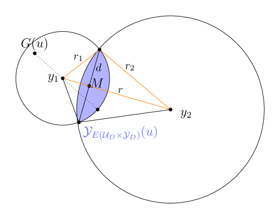
Let $\mathcal{Y}_{E(\mathcal{U}_{D}^{\ell}\times\mathcal{Y}_{D}^{\ell})}(u)$ denote the projection of $E(\mathcal{U}_{D}^{\ell}\times\mathcal{Y}_{D}^{\ell})$ for an input $u\in\mathcal{U}$ on $\mathcal{Y}$, i.e., the set of possible outputs for input $u$ included in $E(\mathcal{U}_{D}^{\ell}\times\mathcal{Y}_{D}^{\ell})$. Since $\mathcal{U}_{D}^{\ell}\times\mathcal{Y}_{D}^{\ell}$ contains two data samples, $\mathcal{Y}_{E(\mathcal{U}_{D}^{\ell}\times\mathcal{Y}_{D}^{\ell})}(u)$ corresponds to the intersection of two $n-1$-dimensional spheres with center $y_{1}$ and $y_{2}$, respectively, and radius $r_{1}(u)$ and $r_{2}(u)$, respectively. Due to the Lipschitz continuity of $N$, $\mathcal{Y}_{E(\mathcal{U}_{D}^{\ell}\times\mathcal{Y}_{D}^{\ell})}(u)$ is non-empty and contains a $n-2$ dimensional sphere with diameter $2d(u)$ and center $M(u)$. To derive the upper bound (7), we bound the distance of $G(u)$ to all outputs in $\mathcal{Y}_{E(\mathcal{U}_{D}^{\ell}\times\mathcal{Y}_{D}^{\ell})}(u)$. To this end, we distinguish between three possible cases depending on the location of the center $M(u)$ and then take the maximum over those cases as in (7).
In the first case, the center $M(u)$ lies between $y_{1}$ and $y_{2}$ as depicted in Figure 3.

Figure 3: Set of possible outputs $\mathcal{Y}_{E(\mathcal{U}_{D}^{\ell}\times\mathcal{Y}_{D}^{\ell})}(u)$ by Lipschitz continuity at two samples. The case with center $M(u)$ between the output samples $y_{1}$ and $y_{2}$.

Since the distance of $M(u)$ to any point in $\mathcal{Y}_{E(\mathcal{U}_{D}\times\mathcal{Y}_{D})}(u)$ is less than or equal to the half of the diameter $2d(u)$, the triangle inequality yields

$$\max_{y\in\mathcal{Y}_{E(\mathcal{U}_{D}^{\ell}\times\mathcal{Y}_{D}^{\ell})}(u)}||y-G(u)||\leq||M(u)-G(u)||+d(u)$$

which corresponds to $\alpha_{\text{AE}}^{E(\mathcal{U}_{D}^{\ell}\times\mathcal{Y}_{D}^{\ell}),G}$.
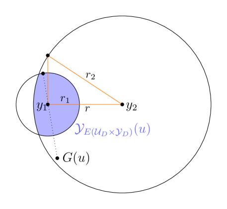
The second case is depicted in Figure 4 where the center $M(u)$ doesn’t lie between $y_{1}$ and $y_{2}$ or even one sphere is completely included in the other.

Figure 4: Set of possible outputs $\mathcal{Y}_{E(\mathcal{U}_{D}^{\ell}\times\mathcal{Y}_{D}^{\ell})}(u)$ by Lipschitz continuity at two samples. The case with center $M(u)$ not between the output samples $y_{1}$ and $y_{2}$.

This case is characterized by $r_{2}(u)^{2}\geq r_{1}(u)^{2}+r(u)^{2}$ if $y_{1}$ lies in $\mathcal{Y}_{E(\mathcal{U}_{D}^{\ell}\times\mathcal{Y}_{D}^{\ell})}(u)$ (by $r_{1}(u)^{2}\geq r_{2}(u)^{2}+r(u)^{2}$ if $y_{2}$ lies in $\mathcal{Y}_{E(\mathcal{U}_{D}^{\ell}\times\mathcal{Y}_{D}^{\ell})}(u)$) as follows from the orange triangle in Figure 4. Since $y_{1}$ ($y_{2}$) lies in $\mathcal{Y}_{E(\mathcal{U}_{D}^{\ell}\times\mathcal{Y}_{D}^{\ell})}(u)$,

$$\max_{y\in\mathcal{Y}_{E(\mathcal{U}_{D}\times\mathcal{Y}_{D})}(u)}||y-G(u)||\leq||y_{1(2)}-G(u)||+r_{1(2)}(u)$$

based on the triangle inequality. This results in $\beta_{\text{AE}}^{E(\mathcal{U}_{D}\times\mathcal{Y}_{D}),G}$ ($\gamma_{\text{AE}}^{E(\mathcal{U}_{D}\times\mathcal{Y}_{D}),G}$). ∎

Although the relaxation from Theorem 5 is nonconvex, the complexity of its optimization problems (7) is significant lower compared to (6) as the optimization over $y\in\mathbb{R}^{n}$ is avoided. Therefore, the relaxation (7) requires the optimization of $\mu$ variables because the input set $\mathcal{U}$ is spanned by a $\mu$-dimensional orthonormal basis (1).
So far the output trajectories of $\mathcal{Y}_{D}$ are assumed to be measured without noise. However, we can adapt the envelope $E(\mathcal{U}_{D}\times\mathcal{Y}_{D})$ and the presented relaxation to provide a guaranteed upper bound on the AE-NLM for noisy measurements as shown in the next remark.

Remark 6.

If the measured output $\tilde{y}$ of the system $N(u)$ is corrupted by additive and bounded noise $v$, i.e.,

$$\tilde{y}=N(u)+v,\quad v^{T}v\leq\delta^{2},$$

then the Lipschitz continuity implies

$$||N(u^{\prime})-\tilde{y}||\leq L||u^{\prime}-u||+\delta.$$

Hence, we increase the radii $r_{1}(u)$ and $r_{2}(u)$ in Theorem 5 by $\delta$ to ensure a guaranteed upper bound on the AE-NLM. Analogously, if the noise exhibits a signal-to-noise-ration $\delta$, i.e., $v^{T}v\leq\delta^{2}y^{T}y$, then the Lipschitz continuity and the assumption $N(0)=0$ imply

$$||v||^{2}\leq\delta^{2}||N(u)||^{2}\leq\delta^{2}L^{2}||u||^{2}\leq\delta^{2}L^{2}||u_{H}||^{2},$$

where $u_{H}$ denotes the largest input of the considered subset of the partition with respect to the Euclidean norm. Thereby, we increase the radii $r_{1}(u)$ and $r_{2}(u)$ by $\delta L||u_{H}||$.

IV-B Iterative scheme for AE-NLM inference

In the previous section, local inferences and a nonconvex relaxation are studied to derive the (global) inference of the AE-NLM (4) for given data samples. To improve the guaranteed upper bound, further experiments can be evaluated iteratively on the plant. We establish in the following such an iterative procedure similar to a branch-and-bound algorithm.

Algorithm 7 (Iterative scheme for AE-NLM inference).

• Suppose a set of input-output samples are given. Initially, compute the linear approximation model $G$ that minimizes the maximal distance to the data samples according to the semidefinite-program in [3]. Moreover, define a partition of $\bar{\mathcal{U}}$ by hyperrectangles $\bar{\mathcal{U}}_{H_{1}},\dots,\bar{\mathcal{U}}_{H_{h}}$ and compute the local AE-NLM inference (6) and its maximizing ‘worst-case’ input for all $\bar{\mathcal{U}}_{H_{i}},i=1,\dots,h$. Set the number of iterations $k$ to zero.

• Identify the hyperrectangle $\bar{\mathcal{U}}_{H_{i^{*}}}$ with the largest local AE-NLM inference ${\Phi_{\text{AE}}^{\mathcal{U},G*}}$ and add this to the sequence $\Phi_{\text{AE}}^{\mathcal{U},G}(0),\dots,\Phi_{\text{AE}}^{\mathcal{U},G}(k):=\Phi_{\text{AE}}^{\mathcal{U},G*}$. Moreover, add the corresponding ‘worst-case’ amplitudes $\bar{u}^{*}\in\bar{\mathcal{U}}_{H^{*}}$ to the sequence $\bar{u}^{*}(0),\dots,\bar{u}^{*}(k):=\bar{u}^{*}$.

• Divide hyperrectangle $\bar{\mathcal{U}}_{H_{i^{*}}}$ into two hyperrectangles $\bar{\mathcal{U}}^{1}_{H_{i^{*}}}$ and $\bar{\mathcal{U}}^{2}_{H_{i^{*}}}$ by a $\mu-1$ dimensional hyperplane which is orthogonal to one dimension and divides the largest edge of $\bar{\mathcal{U}}_{H_{i^{*}}}$. Moreover, the hyperplane contains

  • $\bar{u}^{*}$ if $1/\alpha<\text{vol}(\bar{\mathcal{U}}^{1}_{H_{i^{*}}})/\text{vol}(\bar{\mathcal{U}}^{2}_{H_{i^{*}}})<\alpha$ for some chosen $\alpha>0$;

  • else the middle point of $\bar{\mathcal{U}}_{H_{i^{*}}}$.

• Determine the output of the plant for

  • $\bar{u}^{*}$ in case of 3a);

  • the middle point of $\bar{\mathcal{U}}_{H_{i^{*}}}$ in case of 3b).

• Compute the local inference of the AE-NLM for hyperrectangles $\bar{\mathcal{U}}^{1}_{H_{i^{*}}}$ and $\bar{\mathcal{U}}^{2}_{H_{i^{*}}}$. Saturate these local AE-NLM inferences by the local inference of $\bar{\mathcal{U}}_{H_{i^{*}}}$.

• Set $\bar{\mathcal{U}}_{H_{i^{*}}}:=\bar{\mathcal{U}}^{1}_{H_{i^{*}}}$, $\bar{\mathcal{U}}_{H_{h+1}}=\bar{\mathcal{U}}^{2}_{H_{i^{*}}}$, $h:=h+1$, and $k:=k+1$. Go to Step 2).

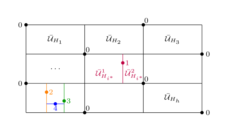
An illustration of Algorithm 7 is depicted in Figure 5.

Figure 5: Schematic illustration of the sampling procedure of the input space $\bar{\mathcal{U}}$ by Algorithm 7. The numbers indicate the sampling in iteration $k$.

In the sequel, we comment on Algorithm 7 and on some properties of Algorithm 7 more thoroughly.
In step 3), we suggest one, among others, proceedings for dividing the hyperrectangle $\bar{\mathcal{U}}_{H^{*}}$. In particular, the decision between 3a) and 3b) is required to prove convergence of the sequence $\Phi_{\text{AE}}^{\mathcal{U},G}(0),\Phi_{\text{AE}}^{\mathcal{U},G}(1),\dots$ to the true AE-NLM in Theorem 8. Furthermore, the new evaluated input from step 4) is taken into account in the computation of the local AE-NLM inferences in step 5) since its distance to the new hyperrectangles is zero.
First property of Algorithm 7 is that its complexity does not increase with further iterations, as the local AE-NLM inference (6) of two hyperrectangles is computed in each iteration. Hence, stopping the iteration after some iterations due to too large computation time won’t occur once the algorithm can be initialized. Second, the sequence of global inferences $\Phi_{\text{AE}}^{\mathcal{U},G}(\cdot)$ from step 2) is monotone decreasing, as the local AE-NLM inferences of the hyperrectangles $\bar{\mathcal{U}}^{1}_{H_{i^{*}}}$ and $\bar{\mathcal{U}}^{2}_{H_{i^{*}}}$ are saturated by the local inference of $\bar{\mathcal{U}}_{H_{i^{*}}}$. Without saturation, the sequence could increase as the envelopes considered for $\bar{\mathcal{U}}^{1}_{H_{i^{*}}}$ and $\bar{\mathcal{U}}^{2}_{H_{i^{*}}}$, respectively, are not necessarily a subset of the envelope considered for $\bar{\mathcal{U}}_{H_{i^{*}}}$. Finally, the sequence of global inferences $\Phi_{\text{AE}}^{\mathcal{U},G}(\cdot)$ converges to the true AE-NLM as proven in the following theorem.

Theorem 8 (Convergence).

The sequence of global inferences of the AE-NLM $\Phi_{\text{AE}}^{\mathcal{U},G}(\cdot)$ from step 2) of Algorithm 7 converges to the solution of the left-hand side of (3), i.e.,

$$\lim_{k\rightarrow\infty}\Phi_{\text{AE}}^{\mathcal{U},G}(k)=\Phi^{\mathcal{U},G}_{\text{AE}}.$$

Proof.

The sequence $\Phi_{\text{AE}}^{\mathcal{U},G}(\cdot)$ is lower bounded by zero and non-increasing which implies its convergence. We suppose that the sequence $\Phi_{\text{AE}}^{\mathcal{U},G}(\cdot)$ doesn’t converge to $\Phi^{\mathcal{U},G}_{\text{AE}}$. Thus, the sequence of corresponding ‘worst-case’ inputs ${u}^{*}(\cdot)\in\mathcal{U}$ from step 2) doesn’t converge to the set of inputs ${\mathcal{U}}^{*}\subset{\mathcal{U}}$ which solve the left-hand side of (3), but to a subset ${\mathcal{U}}_{c}\nsupseteq{\mathcal{U}}^{*}$. Due to the convergence to ${\mathcal{U}}_{c}$, the distinction of 3a) and 3b), and the sampling in step 4), we can choose ${\mathcal{U}}_{c}$ such that the radii $r_{1}(u)$ and $r_{2}(u)$ from relaxation (7) for each subset ${\mathcal{U}}_{H_{i}}\subseteq{\mathcal{U}}_{c}$ are bounded by an arbitrary small $\rho>0$, i.e.,

$$\max\{r_{1}(u),r_{2}(u)\}<\rho$$

for all $u\in{\mathcal{U}}_{H_{i}}$ and all subsets ${\mathcal{U}}_{H_{i}}\subseteq{\mathcal{U}}_{c}$. Therefore, the local inference of the AE-NLM (6) using the relaxation (7) is bounded from above by

$$\max_{\begin{subarray}{c}u\in\mathcal{U}_{H_{i}},||u||\geq\epsilon,\\ i=1,2\end{subarray}}\frac{||y_{i}-G(u)||+\rho}{||u||}$$ (8)

for each subset ${\mathcal{U}}_{H_{i}}\subseteq{\mathcal{U}}_{c}$. The convergence

$$\lim_{\rho\rightarrow 0}\max_{\begin{subarray}{c}u\in\mathcal{U}_{H_{i}},||u||\geq\epsilon,\\ i=1,2\end{subarray}}\frac{||y_{i}-G(u)||+\rho}{||u||}=\frac{||y_{1}-G(u_{1})||}{||u_{1}||}$$

implies that $\rho$ can be chosen small enough such that (8) is for all ${\mathcal{U}}_{H_{i}}\subseteq{\mathcal{U}}_{c}$ less than

$$\frac{||N({u}^{*})-G(u^{*})||}{||{u}^{*}||},{u}^{*}\in{\mathcal{U}}^{*}.$$

Together with the search for the largest local AE-NLM inference in step 2) of Algorithm 7, this leads to a contradiction for the convergence of the sequence ${u}^{*}(\cdot)\in\mathcal{U}$ to ${\mathcal{U}}_{c}\nsupseteq{\mathcal{U}}^{*}$. Hereby, the sequence ${u}^{*}(\cdot)$ converges to ${\mathcal{U}}^{*}$, and therefore $\Phi_{\text{AE}}^{\mathcal{U},G}(\cdot)$ to $\Phi^{\mathcal{U},G}_{\text{AE}}$. ∎

V Numerical Example

In this section, we apply Algorithm 7 to conclude on the AE-NLM of the input-output behaviour of the SISO system

$$\dot{x}_{1} =-3x_{1}+4x_{2}+2x_{1}^{2}-0.2\sin(3x_{1})+u,$$

$$\dot{x}_{2} =-x_{1}+0.6x_{2}-0.5x_{1}^{3},\quad x(0)=0,$$

$$y =x_{1}.$$

The discrete-time input-output trajectories are drawn based on simulations for 30 time steps by Euler integration with $\Delta t=0.2\,\text{s}$. Similar to [3], the input set is spanned by

$$\mathcal{U}{=}\{u\in\mathbb{R}^{n}:u{=}\sum_{i=1}^{2}\alpha_{i}\frac{v_{i}}{||v_{i}||},(\alpha_{1},\alpha_{2})\in[0,4]^{2}\backslash[0,0.1]^{2}\},$$

where $v_{1}$ and $v_{2}$ denote the stacked time-samplings of the basis signals $v_{1}(t)=\sin(\pi/3t)$ and $v_{2}(t)=\sin(\pi t)$. The Lipschitz constant is estimated to $L=1.04$. Algorithm 7 is initialized by the computation of a linear approximation model described by a lower Toeplitz matrix for 20 samples. The free parameter $\alpha$ of Algorithm 7 is chosen to $0.1$.
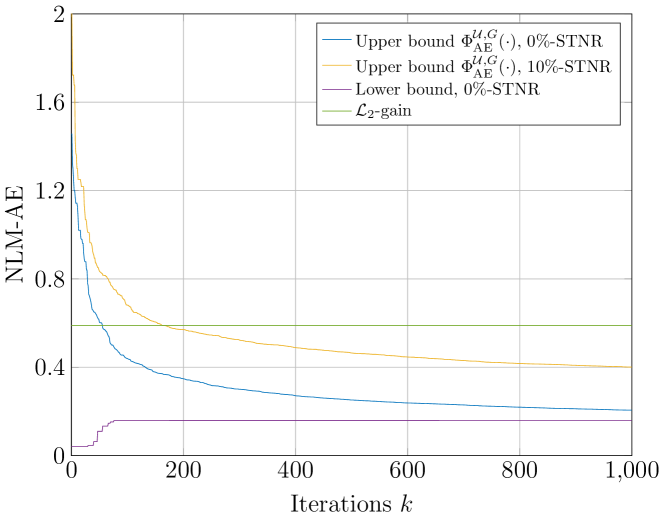
Figure 6 shows the simulated sequence of AE-NLM inferences $\Phi_{\text{AE}}^{\mathcal{U},G}(\cdot)$ of Algorithm 7.

Figure 6: Simulated sequence of AE-NLM inference $\Phi_{\text{AE}}^{\mathcal{U},G}(\cdot)$ of Algorithm 7.

If the output is corrupted by additive noise with a signal-to-noise-ratio of $10\%$, then the adapted Algorithm 7 as described in Remark 6 still provides a guaranteed upper bound of the AE-NLM.
Furthermore, Figure 6 shows the lower bound from [3] on the AE-NLM derived from the collected data. The knowledge of the distance of the guaranteed lower and upper bound on the AE-NLM in each iteration constitutes a reasonable termination criterion for the iteration. Indeed, this distance measures the potential improvement of the AE-NLM estimation by further sampling.
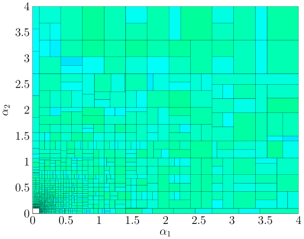
Figure 7 demonstrates the division of the input set $\bar{\mathcal{U}}$ into hyperrectangles by Algorithm 7.

Figure 7: Divided input set $\bar{\mathcal{U}}$ after $1000$ iterations. The colour encodes the relation $\Phi_{\text{AE}}^{\mathcal{U}_{H_{i}},G}/\ell_{2}$ which is smaller than or equal to $1$ by definition.

Due to the iterative approach, Algorithm 7 is more data-efficient than the offline approach [3] that requires $10000$ data samples to conclude on an upper bound of $0.48$ for the AE-NLM. Moreover, the computation time of Algorithm 7 for $1000$ iterations lasts around $5$ minutes which is comparable to [3].

VI Conclusions

In this paper, we exploited a non-parametric data-based set-membership representation of the input-output mapping of an unknown nonlinear system to derive a conclusion on its strength of nonlinearity. First, we concluded on the nonlinearity measure from given input-output samples using local inference of the nonlinearity measure and a nonconvex relaxation. Second, an iterative scheme was presented to decrease the guaranteed upper bound of the AE-NLM by further performed experiments. We ensured that the complexity of each iteration of the algorithm does not increase and proved the convergence to the true nonlinearity measure. In a numerical example, the presented algorithm was more data efficient than the approach in [3].
In a future work, other dissipativity properties could be studied, the iterative scheme could be extended by an alternating optimization [17] of the linear approximation model, and the estimation of the local inference could be improved by considering local Lipschitz constants.

References

• [1] Z. S. Hou and Z. Wang. From model-based control to data-driven control: Survey, classification and perspective. Information Sciences, 235, 3-35, 2013.
• [2] J. M. Montenbruck and F. Allgöwer. Some Problems Arising in Controller Design from Big Data via Input-Output Methods. In Proc. 55th IEEE Conf. on Decision and Control, pp. 6525-6530, 2016.
• [3] T. Martin and F. Allgöwer. Nonlinearity measures for data-driven system analysis and control. In Proc. 58th IEEE Conf. on Decision and Control, pp. 3605-3610, 2019.
• [4] F. Allgöwer. Definition and Computation of a Nonlinearity Measure. In Proc. 3rd IFAC Nonlinear Control Syst. Design Symp., pp. 257-262, 1995.
• [5] T. Schweickhardt and F. Allgöwer. On System Gains, Nonlinearity Measures, and Linear Models for Nonlinear Systems. IEEE Trans. Automatic Control, 54(1):62-78, 2009.
• [6] B. Wahlberg, M. B. Syberg and H. Hjalmarsson. Non-parametric methods for 2subscript2\mathcal{L}_{2}-gain estimation using iterative experiments. Automatica, 46(8):1376-1381, 2010.
• [7] T. Martin, A. Koch and F. Allgöwer. Data-driven surrogate models for LTI systems via saddle-point dynamics. In Proc. 21st IFAC World Congress, 2020.
• [8] C. E. Rasmussen and C. K. I. Williams. Gaussian Processes for Machine Learning. The MIT Press, 2006.
• [9] M. Milanese and C. Novara. Set Membership identification of nonlinear systems. Automatica, 40(6):957–975, 2004.
• [10] J. P. Calliess. Conservative decision-making and inference in uncertain dynamical systems. University of Oxford, 2014.
• [11] A. Blaas, J. M. Manzano, D. Limon and J. Calliess. Localised Kinky Inference. In Proc. 18th European Control Conference (ECC), pp. 985–992, 2019.
• [12] A. H. Land and A. G. Doig. An Automatic Method of Solving Discrete Programming Problems. Econometrica, 28(3):497-520, 1960.
• [13] G. Zames. On the Input-Output Stability of Time-Varying Nonlinear Feedback Systems. Part I: Conditions Derived Using Concepts of Loop Gain, Conicity, and Positivity. IEEE Trans. Automat. Control, 11(2):228-238, 1966.
• [14] R. G. Strongin. On the convergence of an algorithm for finding a global extremum. Engineering in Cybernetics, 1973.
• [15] J. P. Calliess. Lipschitz optimisation for Lipschitz interpolation. In Proc. American Control Conference (ACC), pp. 3141–3146, 2017.
• [16] S. H. Nair, M. Bujarbaruah, and F. Borrelli. Modeling of Dynamical Systems via Successive Graph Approximations. In Proc. 21st IFAC World Congress, 2020. (arXiv preprint, arXiv:1910.03719).
• [17] S. Boyd, N. Parikh, E. Chu, B. Peleato, and J. Eckstein. Distributed Optimization and Statistical Learning via the Alternating Direction Method of Multipliers. Foundations and Trends in Machine Learning, 3(1):1–122, 2010.