Stochastic resetting with stochastic returns using external trap

Abstract

In the past few years, stochastic resetting has become a subject of immense interest. Most of the theoretical studies so far focused on instantaneous resetting which is, however, a major impediment to practical realisation or experimental verification in the field. This is because in the real world, taking a particle from one place to another requires finite time and thus a generalization of the existing theory to incorporate non-instantaneous resetting is very much in need. In this paper, we propose a method of resetting which involves non-instantaneous returns facilitated by an external confining trap potential $U(x)$ centered at the resetting location. We consider a Brownian particle that starts its random motion from the origin. Upon resetting, the trap is switched on and the particle starts experiencing a force towards the center of the trap which drives it to return to the origin. The return phase ends when the particle makes a first passage to this center. We develop a general framework to study such a set up. Importantly, we observe that the system reaches a non-equilibrium steady state which we analyze in full details for two choices of $U(x)$, namely, (i) linear and (ii) harmonic. Finally, we perform numerical simulations and find an excellent agreement with the theory. The general formalism developed here can be applied to more realistic return protocols opening up a panorama of possibilities for further theoretical and experimental applications.

1 Introduction

The subject of resetting or restart has recently taken the center stage due to its myriad of applications in statistical physics [1, 2, 3, 4, 5, 6, 7, 8, 9, 10, 11, 12, 13, 14, 15], in chemical and biological physics [16, 17, 18, 19], in computer science [20, 21], and in search theory [22, 23, 24, 25, 26] (see [28] for a broad review of the topic). Resetting is a simple mechanism where one intermittently stops an ongoing dynamics only to start over again. Despite its simple enough implementation, there has been a surge of rigorous theoretical investigations to understand the effect of resetting on generic stochastic processes. In this context, there are many different aspects that have been studied under the umbrella of non-equilibrium phenomena including stationary states and first passage problems. As an example, consider the paradigmatic model of diffusion in the presence of resetting [1]. In this model, it has been shown that resetting renders a non-equilibrium steady state even though the underlying process i.e., a simple diffusion without resetting is non-stationary. Similar observation along with interesting relaxation phenomena were also made in other stochastic processes, namely anomalous diffusion [31, 32], fractional Brownian motion [33], scaled Brownian motion [34], continuous time random walk [35, 36], Lévy flights [37], and extended systems with many degrees of freedom [38, 39, 40, 41]. While appropriate resetting mechanism can possibly make a non-stationary process stationary, in the context of first passage time problems it has been shown that resetting mechanisms have dramatic consequences on the completion times of stochastic processes. In particular, repeated resetting can facilitate the completion of an arbitrary complex process [1, 2, 8, 22, 25, 28, 42, 43, 44, 45, 46, 47, 48, 49] and this has lead to the major challenging questions such as improvement of the search protocols using resetting [8, 43], existence of an optimal resetting protocol [8, 25, 43] and the universal properties associated to such optimal protocol [42, 46, 50].

Most of the studies on stochastic processes with resetting unequivocally assume the resetting mechanism to be instantaneous. For example, consider the paradigmatic model of diffusion with resetting where the particle is relocated to the initial configuration in zero time [1, 2, 28]. However, these underlying assumptions are often over simplified since in reality the particle will require certain amount of time to return. Thus, new formulations need to be more realistic and physically amenable to include such possibilities into account. Moreover, physical intuition tells us that the return time of the particle will typically depend on its current location, and also on other environmental parameters during its return. A few initial attempts in this direction have recently been proposed in [26, 27] and other consecutive studies [51, 52, 53, 54] where the returns were considered to be non-instantaneous but deterministic. Examples include, return by a constant or spatially homogeneous velocity [51, 52, 53, 54], return in certain time [55] or by means of other deterministic motions [53]. Only recently, experiments using optical tweezers have been performed to realize such protocols [29, 30].

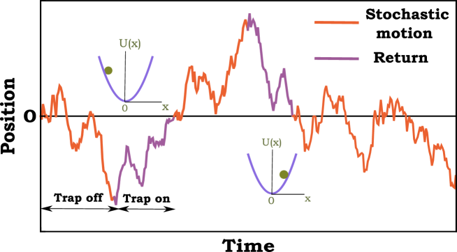
Figure 1: Schematic trajectory of a particle undergoing a stochastic motion phase (e.g., free diffusion) followed up by a return phase modulated by an optical trap which is centered at the origin. The trap creates an attractive potential $U(x)$ around its center. The trap is activated at the time of resetting, which occurs at random with rate $r$, and kept ‘on’ until the particle returns to the origin for the first time. Once the particle hits the origin, the potential is switched ‘off’ and the particle resumes its stochastic motion phase.

We consider the following protocol: assume that a particle starts a random motion (phase I) from the origin at time zero. It explores around until a resetting occurs after some random interval of time and consequently the particle is required to return to the origin (for simplicity we set the initial position same as the resetting position). This phase is called the return phase (phase II). In this phase the motion of the particle is manipulated externally by turning an external confining potential on. Such confining potential can be achieved in experiments using the optical trap technique [56]. The trap (often modelled as harmonic potential in theory) is set up so that its minimum is at the origin and it is switched on only during phase II. When active (i.e., on), the trap generates an attractive force field towards its center (the origin), and hence the particle will diffuse downhill (phase II - return). We observe the motion until the particle hits the origin for the first time. At this very moment, the trap is switched off and the particle resumes its exploring phase motion i.e., phase I motion (see figure 1 for a typical trajectory). It is easy to realise that the compound process is recurrent and in the long time the particle will reach a non-equilibrium steady state. In this paper, we are interested in the distribution of the position of the particle in this steady state.

The remainder of the paper is organized as follows. We provide the details of our set-up in section 2. In the next section (section 3) we develop a general theory which characterizes such set up within a broad framework. Sec. 4 is devoted to the analysis of the non-equilibrium stationary state. We then apply our framework to some realistic situations, and derive exact results in section 5. We conclude the paper in section 6 with discussions and possible future directions.

2 Set up

We consider a set up in one-dimension in which a particle starts to evolve from the origin at time zero. Motion of the particle is governed by a two-phase compound process. In the first phase, the particle performs motion according to some stochastic process. In the second phase it returns to its initial position with the aid of an external force exerted by the optical trap. A typical trajectory of such a compound process is shown in figure 1. In the following, we describe each of the phases in details.

Phase I - Stochastic motion and resetting: We assume that the first phase of stochastic motion of the particle can be described by a Fokker-Planck equation

$$\partial_{t}\rho_{0}(x,t)=\mathcal{L}_{0}\rho_{0}(t)~{},$$ (1)

where $\mathcal{L}_{0}$ is the generator of the stochastic process and $\rho_{0}(x,t)$ is the propagator that describes the particle’s motion when observed in the absence of resetting. To understand the mechanism of stochastic resetting let us briefly discuss the case of instantaneous resetting in which at any small interval $dt$, the particle is instantaneously teleported to the origin with probability $rdt$. In other words, the waiting times between resetting events is drawn from an exponential distribution $f(t)=re^{-rt}$. The corresponding master equation reads [1, 2, 7]

$$\partial_{t}\rho_{\text{inst}}(x,t)=\mathcal{L}_{0}\rho_{\text{inst}}(x,t)-r\rho_{\text{inst}}(x,t)+r\delta(x)~{},$$ (2)

where $\rho_{\text{inst}}(x,t)$ is the propagator for such a process. Stochastic processes with instantaneous resetting have been studied in great details. Here we consider the situation where the particle takes non-zero time to return to the origin. This will be discussed in the following.

Phase II - Return: As done in the context of instantaneous resetting, after a random time interval $t$ drawn from the exponential distribution $f(t)$, motion of the particle changes from phase I to phase II. In this phase, the particle is facilitated to return to the origin by switching on an external confining potential $U(x)$. The center of the trap is situated at the resetting location (same as the initial position and set at the origin). Thus, the particle will diffuse in the force field $F(x)$ generated by the potential $U(x)$ and eventually will reach at the minimum of the trap. The first time the particle reaches to the center (origin), the trap is switched off and this marks the end of phase II. Upon return to the origin, the particle momentarily restarts its motion in phase I. Therefore, we have a compound event or a trial which comprises of the stochastic motion in phase I until the resetting epoch followed by a first passage to the center of the trap in phase II. Each trial repeats by itself along a long trajectory and is essentially a renewal process. We mention that similar switching ‘on’ and ‘off’ of external potentials is also used in ratchet problems [57], albeit with an important difference. There, switching between ‘on’ and ‘off’ states of the potential are usually controlled by external agents, whereas in our set up this depends entirely on the motion of the particle in the potential in phase II. In the next section we provide a general formalism of stochastic resetting under stochastic returns.

3 General theory

In this section, we will construct a set of master equations, similar to (2), to describe the full dynamics of our system.

3.1 Dynamical equations for motion and return density

We assume that the particle, starting from the origin, performs simple diffusion (with diffusion constant $D$) in phase I and upon resetting it returns to the origin via diffusion in the force field $F(x)$ with a different diffusion constant $D_{R}$. Although in any experimental set up it is reasonable to consider $D_{R}=D$, we, however, proceed with $D_{R}\neq D$ to keep our framework more general.

Let, $\rho_{M}(x,t)$ and $\rho_{R}(x,t)$ be the probability densities for the position of the particle at time $t$ during the stochastic motion (M - phase I) and the return (R - phase II) phases, respectively. Thus the full density $\rho(x,t)$ of the combined process is given by

$$\rho(x,t)=\rho_{M}(x,t)+\rho_{R}(x,t)~{},$$ (3)

which consists of two parts with respective contributions from each phase. It is evident that $\rho_{M}(x,t)$ and $\rho_{R}(x,t)$ are not individually normalized as their sum is the total probability density $\rho(x,t)$ which is normalized to one. The probabilities to find the particle in the stochastic motion (phase I) and return phase (phase II) are respectively given by

$$\begin{split}p_{M}(t)\equiv\text{Prob}(\text{\text{Phase I}})&=\int\limits_{-\infty}^{\infty}dx~{}\rho_{M}(x,t),\\ p_{R}(t)\equiv\text{Prob}(\text{\text{Phase II}})&=\int\limits_{-\infty}^{\infty}dx~{}\rho_{R}(x,t),\end{split}$$ (4)

where $p_{M}(t)+p_{R}(t)=1$ at all times with the initial condition $p_{M}(0)=1$.

We now derive equations for $\rho_{M}(x,t)$ and $\rho_{R}(x,t)$, and thus for the propagator $\rho(x,t)$ which describes our process. We first note that the probability current at $x$ due to returning particles is $J_{R}(x,t)=F(x)\rho_{R}(x,t)-D_{R}\frac{\partial\rho_{R}(x,t)}{\partial x}$. Note that, without loss of generality, we set the friction coefficient to be unity through out the paper. On the other hand, the probability flux at $x$ due to particles which switch from the stochastic motion in phase I to the return phase is given by $r\rho_{M}(x,t)$. Adding these two possibilities gives

$$\partial_{t}\rho_{R}(x,t) = -\partial_{x}J_{R}(x,t)+r\rho_{M}(x,t)-\delta(x)\left[J_{R}(0^{-},t)-J_{R}(0^{+},t)\right]~{},$$ (5)

where the last term on the right hand side serves as a sink and accounts for the fact that the returning particles switch to stochastic motion in phase I as soon as they arrive at the origin. Note that the current at the origin gets contributions from the incoming return particles from both sides, and these two contributions are not necessarily equal in magnitude (in case of asymmetric potential applied in the return phase). Thus in this case $J_{R}(0^{+},t)$ [$J_{R}(0^{-},t)$] is simply the current flowing into the origin from the positive (negative) side on the real axis. We define the net current at the origin as the total probability flux arriving at $x=0$ from both sides, that is, $\overline{J}_{R}(0,t)=J_{R}(0^{-},t)-J_{R}(0^{+},t)$. Thus, we can rewrite (5) as

$$\partial_{t}\rho_{R}(x,t) =-\partial_{x}J_{R}(x,t)+r\rho_{M}(x,t)-\delta(x)\overline{J}_{R}(0,t)$$ (6)

We now turn our attention to the time evolution of the position distribution $\rho_{M}(x,t)$ in phase I. During this phase, the particles will evolve in $dt$ time interval according to the generator of the process $\mathcal{L}_{0}$ with probability $1-rdt$. With the complementary probability, the particles will switch from this phase to the return phase. Accounting for all the contributions, we arrive at the following equation

$$\partial_{t}\rho_{M}(x,t)=\mathcal{L}_{0}\rho_{M}(x,t)-r\rho_{M}(x,t)+\delta(x)\overline{J}_{R}(0,t),$$ (7)

where the second term on the RHS indicates the outward probability from the stochastic motion (phase I). The third term on the RHS acts as a source for the returning particles in phase II which switch to stochastic motion in phase I upon arrival at the origin. Thus, (6) and (7) together with the initial conditions $\rho_{R}(x,0)=0$ and $\rho_{M}(x,0)=\delta(x)$ describe the complete motion of the particle.

3.2 Boundary and matching conditions on the densities

To solve the master equations in phase I and II, one needs to supplement them with appropriate boundary conditions which we discuss in the following. We start by decomposing the return phase density in the following way

$$\rho_{R}(x,t)=\rho_{R}^{-}(x,t)\theta(-x)+\rho_{R}^{+}(x,t)\theta(x)~{},$$ (8)

where $\rho_{R}^{\pm}(x,t)$ correspond to the phase space densities conditioned on the fact that the particles started their return phase motion from $x>0~{}(x<0)$ respectively at the end of phase I and $\theta(x)$ stands for the Heaviside step function. This decomposition is natural since the returning particles can either be in the positive or negative $x$ in each trial. Thus, switching between them is possible only via returns to the origin followed by the phase I. Essentially this implies that $\rho_{R}^{\pm}(x,t)$-s are not directly coupled, but rather coupled through $\rho_{M}(x,t)$. The returning particles, upon reaching at the origin for the first time, switch to phase I. As a result, the origin effectively acts as an absorbing boundary for the return probabilities. Hence, we should have

$$\rho_{R}^{\pm}(0,t)=0~{}.$$ (9)

It should be stressed again that there is no physical absorbing boundary at the origin, but the above conditions are invoked to implement the termination of return phase II at the origin. On the other hand the particles can not get accumulated at the infinity in finite time for motions in both phases I and II. As a result, we have

$$\lim_{x\to\pm\infty}\rho_{R}^{\pm}(x,t)=0,\qquad\lim_{x\to\pm\infty}\rho_{M}(x,t)=0.$$ (10)

Equivalently there can not be any particle current at $x=\pm\infty$ from phases I and II, which implies the following natural boundary conditions

$$\lim_{x\to\pm\infty}J_{R}(x,t)=0,\qquad\lim_{x\to\pm\infty}J_{M}(x,t)=0.$$ (11)

These conditions can also be argued from the more natural boundary conditions i.e., $\lim\limits_{x\to\pm\infty}J_{\text{tot}}(x,t)=0$, where $J_{\text{tot}}(x,t)$ is the total particle current which satisfies the full continuity equation $\partial_{t}\rho(x,t)+\partial_{x}J_{\text{tot}}(x,t)=0$. The above equation is obtained by simply adding (6) and (7). We can therefore write $J_{\text{tot}}(x,t)=J_{R}(x,t)+J_{M}(x,t),$ where $J_{M}(x,t)$ can be understood as the particle current in the phase I motion. A careful observation of (7) tells us that $J_{M}(x,t)$ is not sensitive to the arbitrary choices of the return dynamics in phase II. As a result, the $x$ dependence of $J_{M}(x,t)$ is completely independent from that of $J_{R}(x,t)$. Moreover, one also has the freedom to choose two independent dynamics for the positive and negative $x$ in phase II. Thus, $x$ dependence of $J_{R}(x,t)$ at $x>0$ is also independent from the $x$ dependence of $J_{R}(x,t)$ at $x<0$. Now if $J_{\text{tot}}(x,t)$ vanishes as $x\to\pm\infty$, the individual currents $J_{M}(x,t)$ and $J_{R}(x,t)$ also must go to zero as $x\to\pm\infty$. This provides another justification of the boundary conditions in (11).

Finally, we note that $\rho_{M}(x,t)$ is continuous across the origin implying

$$\rho_{M}(0^{+},t)=\rho_{M}(0^{-},t)~{},$$ (12)

as a matching condition for solving the density in phase I. Since the boundary conditions in Eqs. (9) - (12) are valid at all times, they automatically translate to the steady state.

4 Non-equilibrium steady state

Equations (6) and (7) along with the initial and boundary conditions stated above constitute the central equations that describe a full, time dependent, description of stochastic motion with resetting and space time coupled stochastic returns to the origin. However, solving these equations in full generality seems quite challenging and from now on, we focus only on the steady-state properties of our process.

4.1 Steady state density in phase I

To compute the density in phase I, we first show that the steady state equation (obtained by setting $\partial_{t}\rho_{M}(x,t)=0$ in (7)) for $\rho_{M}(x)$ can be cast into the form satisfied by the steady state density $\rho_{\text{inst}}(x)$ for instantaneous resetting. This can be done by observing that $\overline{\rho}_{M}(x)=\frac{r}{\overline{J}_{R}(0)}\rho_{M}(x)$ satisfies

$$\mathcal{L}_{0}\overline{\rho}_{M}(x)-r\overline{\rho}_{M}(x)+r\delta(x)=0~{},$$ (13)

which has the same form as (2) in steady state. Here $\overline{J}_{R}(0)=\lim_{t\to\infty}\overline{J}_{R}(0,t)$ is the steady state current to the origin. Hence we have

$$\rho_{M}(x)=\frac{\overline{J}_{R}(0)}{r}\rho_{\text{inst}}(x)~{},$$ (14)

which directly implies (after integrating both sides of the above equation over the real axis)

$$\overline{J}_{R}(0)=rp_{M}~{},$$ (15)

where $p_{M}$ (now time independent) is the stationary probability that the particle is in phase I. Substituting this relation in (14), we have

$$\rho_{M}(x)=p_{M}\rho_{\text{inst}}(x)~{}.$$ (16)

It is important to point out that $\rho_{M}(x)=p_{M}\rho(x|\text{phase I})$ where $\rho(x|\text{phase I})$ is the conditional probability density to find the particle at a position $x$ given that it is in phase I. Thus, (16) simply asserts $\rho(x|\text{phase I})=\rho_{\text{inst}}(x)$ which will prove to be a useful relation later. In the next section, we discuss how to obtain the steady state density in phase II.

4.2 Steady state density in return phase

To compute the steady state density in return phase, we proceed as before and set $\partial_{t}\rho_{R}(x,t)=0$ in (6). Further we substitute $\overline{J}_{R}(0)$ from (15) into (6) to obtain

$$D_{R}\frac{\partial^{2}\rho_{R}(x)}{\partial x^{2}}-\frac{\partial}{\partial x}\left[F(x)\rho_{R}(x)\right]+r\rho_{M}(x)-rp_{M}\delta(x)=0~{},~{}\hskip 8.5359pt$$ (17)

which can, in principle, be solved for a given $F(x)$. However, as we have shown earlier $\rho_{R}(x)$ can again be split into the density in positive and negative axis so that

$$\rho_{R}(x)=\rho_{R}^{-}(x)\theta(-x)+\rho_{R}^{+}(x)\theta(x)~{},$$ (18)

where the probabilities on positive and negative $x$, individually satisfy

$$D_{R}\frac{\partial^{2}\rho^{\pm}_{R}(x)}{\partial x^{2}}-\frac{\partial}{\partial x}\left[F(x)\rho^{\pm}_{R}(x)\right]+r\rho_{M}(x)=0.$$ (19)

Applying the boundary conditions as mentioned in section 3.2 and utilizing the form for $\rho_{M}(x)$, we note that the solutions $\rho_{R}(x)$ can be expressed in terms of $p_{M}$. Hence, the remaining task at our disposal is to evaluate $p_{M}$.

4.3 Interpretation of $p_{M}$

There are two different ways to solve for $p_{M}$. In the first method, we simply use the normalization condition for the total probability density i.e.,

$$\int\limits_{-\infty}^{\infty}~{}dx~{}\left[\rho_{M}(x)+\rho_{R}(x)\right]=1~{}.$$ (20)

Since, both the densities individually depend explicitly on $p_{M}$, this condition evaluates $p_{M}$ exactly. However, $p_{M}$ can also be computed in the steady state from the following arguments. Intuitively it is easy to get convinced that $p_{M}$ is, in fact, the fraction of time the particle spends in phase I in the steady-state. For a detailed discussion on this we refer to the previous observations made in [51, 52]. The mean time spent in phase I is $1/r$ (inverse of resetting rate). On the other hand, the time spent while returning to the origin from position $x$ is nothing but the first passage time to the origin i.e.,

$$\tau(x)=[\mathcal{T}=\{\text{inf}:Y(\mathcal{T}|x)=0\}],$$ (21)

where $Y(\mathcal{T}|x)$ depicts the return phase motion which has started from the location $x$ at time zero in its own clock. The return time $\tau(x)$ is a random variable because (i) $x$ is random and determined by the motion in phase I and (ii) motion of the return phase itself is stochastic namely diffusion in a force field. Thus, we first average over the return phase motion given that it started from $x$ — this gives us the mean first passage time $\overline{\tau}(x)$. Performing the second average over $x$, weighted by the conditional distribution in phase I, we obtain the mean time spent in the return phase (or equivalently the mean return time)

$$\langle\overline{\tau}(x)\rangle=\int\limits_{-\infty}^{\infty}~{}\mathrm{d}x~{}\overline{\tau}(x)\rho(x|\text{\text{phase I}})=\int\limits_{-\infty}^{\infty}~{}\mathrm{d}x~{}\overline{\tau}(x)~{}\rho_{\text{inst}}(x)~{}.\hskip 8.5359pt$$ (22)

Thus the total average time for a trial of the compound motion is $1/r+\langle\overline{\tau}(x)\rangle$. Hence, the fraction of time spent in phase I motion in steady state is given by

$$p_{M}=\frac{1/r}{1/r+\langle\overline{\tau}(x)\rangle}~{}.$$ (23)

In A, we have reviewed one of the standard methods to compute the mean first passage time $\overline{\tau}(x)$ and then applied the same to compute the mean return time for two choices of return motions.

5 Applications to linear and quadratic potentials

In this section, we present two exactly solvable models using the general framework presented above. As mentioned earlier, although the formalism described above can be applied to arbitrary Markovian stochastic processes both in phase I and II, we restrict ourselves in this paper to study diffusive processes. More precisely, we consider that in phase I, the particle diffuses freely with diffusion constant $D$, thus $\mathcal{L}_{0}=D\frac{\partial^{2}}{\partial x^{2}}$, and in phase II we assume that the particle returns to the origin using diffusion but now with a different diffusion constant $D_{R}$ in presence of an external confining potential $U(x)$ which applies a force $F(x)=-dU(x)/dx$ on the particle. To compute $\rho_{M}(x)$, we recall from (16) that it is proportional to $\rho_{\text{inst}}(x)$, the steady-state density for diffusion with stochastic resetting and instantaneous returns. This density can be obtained by solving (2) in the steady state and the resulting solution reads [1, 2]

$$\rho_{\text{inst}}(x)=\frac{\alpha}{2}e^{-\alpha|x|}~{},~{}\text{with}~{}~{}~{}\alpha=\sqrt{\frac{r}{D}}~{}.$$ (24)

Inserting $\rho_{\text{inst}}(x)$ from above into (16) we get

$$\rho_{M}(x)=\frac{p_{M}\alpha}{2}e^{-\alpha|x|}.$$ (25)

We now proceed to compute $\rho_{R}(x)$ in the presence of $U(x)$. In this paper, we consider the following two choices for the confining potential: (i) linear potential: $U(x)=[\lambda_{+}\theta(x)+\lambda_{-}\theta(-x)]~{}|x|$, where $\lambda_{\pm}>0$ and (ii) harmonic potential: $U(x)=\frac{1}{2}kx^{2}$ with $k>0$. Upon each resetting, the trap is switched on i.e., the potential $U(x)$ is made active and the particle diffuses under the force field $F(x)=-dU(x)/dx$, which is (i) $F(x)=\lambda_{-}\theta(-x)-\lambda_{+}\theta(x)$ for linear potential and (ii) $F(x)=-kx$ for harmonic potential.

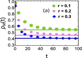
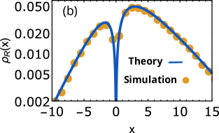
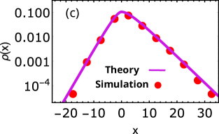
Figure 2: Diffusion and stochastic return under the asymmetric force field: $F(x)=\lambda_{-}\theta(-x)-\lambda_{+}\theta(x)$. Panel (a): Temporal relaxation of $p_{M}(t)$ (starting from $p_{M}(0)=1$) to the steady state, given by (28) and shown by horizontal lines, for three different resetting rates $r=0.1$ (circle), $r=0.2$ (square), and $r=0.3$ (diamond). Panel (b): Comparison of the stationary return density $\rho_{R}(x)$ given by (26) with numerical simulations. Panel (c): Comparison of the total density $\rho(x)$ with the numerical simulations (see B for the details of the simulation methods). In all plots, simulation data are indicated by symbols while the analytical results are shown by solid lines. For panel (b) and (c), we have set $r=0.2$. Values of other common parameters used in all panels are: $D_{R}=1$, $D=1$, $\lambda_{-}=0.75$, and $\lambda_{+}=0.25$. Numerical simulations were performed for $dt=10^{-3}$ and $10^{5}$ realizations.

5.1 Linear potential: $U(x)=[\lambda_{+}\theta(x)+\lambda_{-}\theta(-x)]~{}|x|$

In this case, the particle in phase II experiences a drift $\lambda_{+}(\lambda_{-})$ towards the origin on positive (negative) side of the origin. To compute the steady state density $\rho_{R}^{\pm}(x)$ in the return phase, we now solve (19) with the boundary conditions ((9) and (10)). This yields the following steady state solutions

$$\begin{split}\rho_{R}^{-}(x)&=\frac{rp_{M}}{2}\frac{e^{\alpha x}}{\lambda_{-}-\alpha D_{R}}\left[1-e^{\frac{\lambda_{-}-\alpha D_{R}}{D_{R}}x}\right]~{},\\ \rho_{R}^{+}(x)&=\frac{rp_{M}}{2}\frac{e^{-\alpha x}}{\lambda_{+}-\alpha D_{R}}\left[1-e^{-\frac{\lambda_{+}-\alpha D_{R}}{D_{R}}x}\right]~{}.\end{split}$$ (26)

Combining $\rho_{R}^{-}(x)$ and $\rho_{R}^{+}(x)$ together as in (18) gives us the steady state density $\rho_{R}(x)$ for the particles returning to the origin. In particular, when $\lambda_{-}=\lambda_{+}=\lambda$, the full steady state density (using (18)) in the return phase reads

$$\rho_{R}(x)=\frac{rp_{M}}{2}\frac{e^{-\alpha|x|}}{\lambda-\alpha D_{R}}\left[1-e^{-\frac{\lambda-\alpha D_{R}}{D_{R}}|x|}\right]~{}.$$ (27)

It is evident that the steady state densities $\rho_{M}(x)$ and $\rho_{R}(x)$ in both phases are proportional to the factor $p_{M}$ which now can be computed from the normalization of the total density $\rho(x)$, where $\rho(x)=\rho_{M}(x)+\rho_{R}^{+}(x)\theta(x)+\rho_{R}^{-}(x)\theta(-x)$. This yields

$$p_{M}=\dfrac{2\alpha\lambda_{-}\lambda_{+}}{2\alpha\lambda_{-}\lambda_{+}+r(\lambda_{-}+\lambda_{+})}~{},$$ (28)

which for symmetric force field becomes $p_{M}=\frac{\lambda\alpha}{r+\lambda\alpha}$.

Another way to obtain $p_{M}$ would be to utilize (23) which in turn requires the knowledge of the mean return time $\langle\overline{\tau}(x)\rangle$. For a given starting position $x$, the mean first passage time of a diffusing particle to the origin is given by $\overline{\tau}(x)=|x|\left[\frac{\theta(-x)}{\lambda_{-}}+\frac{\theta(x)}{\lambda_{+}}\right]$ (see A.1 for a detailed calculation). Now performing the average of $\overline{\tau}(x)$ over $\rho_{\text{inst}}(x)$, we find the mean return time: $\langle\overline{\tau}(x)\rangle=\frac{1}{2\alpha}\left(\frac{1}{\lambda_{-}}+\frac{1}{\lambda_{+}}\right)$. Substituting $\langle\overline{\tau}(x)\rangle$ into (23), we recover the same expression for $p_{M}$ in (28) as expected. In figure 2a, we have shown time dependent behavior of $p_{M}(t)$ defined in (4). As can be seen from the figure, $p_{M}(t)$ evolves to its steady state value given by (28). Once $p_{M}$ is known, we have the complete information about the steady state densities. In figure 2b and figure 2c, we observe excellent agreement between the numerical simulation data (see B for the details of the simulation methods) and the theoretical results for the steady state density $\rho_{R}(x)$ (given in (26)) and the total density $\rho(x)=\rho_{M}(x)+\rho_{R}(x)$, respectively, with $\rho_{M}(x)$ given by (25).

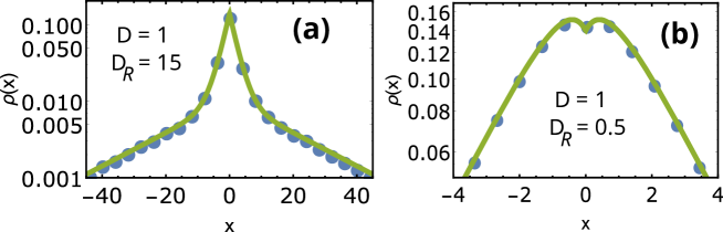
Figure 3: Variation in shapes of $\rho(x)$ in the case of returns towards the origin in presence of symmetric linear potential is shown in corroboration with the simulation data when $D\neq D_{R}$. When $D<D_{R}$, the slope near the origin is negative (panel a) while for $D>D_{R}$ the slope near the origin is positive (panel b). In both cases, the density develops exponential tails far away from the origin. Parameters used in these plots are: $\lambda=0.75,r=0.2$. Numerical simulations were performed for $dt=10^{-3}$ and $10^{6}$ realizations.

Several comments are in order now. The total density exhibits interesting asymptotic behaviors in the limit of small and large $x$. In the following, we furthermore confine our analysis to the symmetric force case i.e., when $\lambda_{\pm}=\lambda$ (however the analysis can be easily generalised to the asymmetric cases). We first discuss the behaviour near $x=0$. Expanding $\rho_{R}(x)$ and $\rho_{M}(x)$ in (27) and (25), respectively, around $x=0$, we get $\rho_{R}(x)\approx\frac{rp_{M}}{2D_{R}}|x|-\frac{rp_{M}(\lambda+\alpha D_{R})}{4D_{R}^{2}}x^{2}$ and $\rho_{M}(x)\approx\frac{\alpha p_{M}}{2}-\frac{\alpha^{2}p_{M}}{2}|x|+\frac{\alpha^{3}p_{M}}{4}x^{2}$ for small $x$. Plugging into the total density we get

$$\rho(x)\approx\frac{\alpha p_{M}}{2}\left[1+\alpha\left(\frac{D}{D_{R}}-1\right)|x|\right]+\frac{\alpha^{2}p_{M}x^{2}}{4}\left[\alpha\left(1-\frac{D}{D_{R}}\right)-\frac{\lambda D}{D_{R}^{2}}\right]~{},$$ (29)

for small $x$. Note that when $D=D_{R}$, the linear term in $\rho(x)$ does not contribute and the profile is parabolic near the origin as shown in figure 2c. On the other hand, when $D\neq D_{R}$, the linear term survives developing a cusp at the origin. See figure 3 where we have plotted the steady state for $D<D_{R}$ (panel a) and $D>D_{R}$ (panel b). The cusp at the origin is clearly visible and the slope near the origin then depends on the ratio $D/D_{R}$.

The large $x$-behavior of the densities depends on both $\lambda$ and $\alpha D_{R}$. For $\lambda/D_{R}>\alpha$, the total density behaves as

$$\rho(x)\approx\frac{\alpha p_{M}}{2}\left[1+\frac{\alpha D}{\lambda-\alpha D_{R}}\right]e^{-\alpha|x|}~{}.$$ (30)

Thus the tail is controlled by the length scale $\alpha^{-1}$, which is the typical (also average) distance traversed by the particle in phase I. On the other hand in the limit $\lambda/D_{R}<\alpha$, the total density behaves as

$$\rho(x)\approx\frac{\alpha p_{M}}{2}\left[\frac{\alpha D}{\alpha D_{R}-\lambda}\right]e^{-\frac{\lambda}{D_{R}}|x|}~{},$$ (31)

where the tail is effected by the factor $\lambda/D_{R}$. This exponential behaviour is verified numerically in figure 3a.

In summary, we find that near the origin, the total density has either linear or quadratic behavior while in the large $x$, the densities have exponential tails. The analysis above holds when $\lambda\neq\alpha D_{R}$. However, the singular limit $\lambda\to\alpha D_{R}$ has to be treated carefully. In this limit, we find that the return density from (27) simplifies to $\rho_{R}(x)=\frac{rp_{M}~{}}{2D_{R}}|x|e^{-\alpha|x|}$. Nevertheless, the asymptotic behaviour of $\rho(x)$ for small $x$ and large $x$ remains same as before.

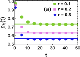
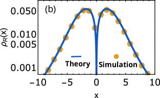
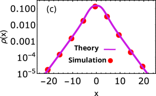
Figure 4: Diffusion and stochastic return under the force field $F(x)=-kx$. Panel (a): Temporal relaxation of $p_{M}(t)$ (starting from $p_{M}(0)=1$) to the steady state values (computed from the theory and shown by solid horizontal lines) for three different resetting rates $r=0.1$ (circle), $r=0.2$ (square), and $r=0.3$ (diamond). Panel (b) and panel (c) respectively compare theoretical expressions for the steady state return density $\rho_{R}(x)$ (given by (36)) and total density $\rho(x)$ with the simulation data (see B for the details of the simulation methods). In all plots, simulation points are denoted by symbols while the theory results are indicated by solid lines. We have set $r=0.2$ in panel (b) and panel (c). In all panels, we have used the following set of parameters: $D_{R}=1$, $D=1$, and $k=0.3$. Numerical simulations were done for $dt=10^{-3}$, and $10^{5}$ (panel a), $10^{6}$ (panel b & panel c) realizations respectively.

5.2 Harmonic potential: $U(x)=kx^{2}/2$

We now consider the case when the return process is driven by the harmonic potential $U(x)=\frac{1}{2}kx^{2}$. Such harmonic potential is possible to realize in experiments using the standard optical trap technique [56]. As mentioned before, in this case also the steady density for the particles diffusing freely in phase I is given by (25). On the other hand, governing equations for the returning particles follow from (19)

$$-\partial_{x}\left[J_{R}^{\pm}(x)\right]+r\rho_{M}(x)=0~{},$$ (32)

where

$$J_{R}^{\pm}(x)=-kx\rho^{\pm}_{R}(x)-D_{R}\frac{\partial\rho^{\pm}_{R}(x)}{\partial x}~{},$$ (33)

are the probability currents in the return phase. We present the solutions for $\rho_{R}(x)$ in the positive $x$-axis. The solutions in the negative $x$-axis will be identical due to the underlying symmetry of the problem. We start by integrating (32) along with (33) on the positive $x$-axis. This gives

$$J_{R}^{+}(x)=c_{2}-\frac{rp_{M}}{2}e^{-\alpha x}~{},$$ (34)

where $c_{2}$ is a constant and is found to be zero by setting the boundary condition $J_{R}^{+}(x\to\infty)=0$ (see section 3.2). To solve the resulting equation for the current $J_{R}^{+}(x)=-\frac{rp_{M}}{2D_{R}}e^{-\alpha x}$, we explicitly use (33) and find

$$\rho_{R}^{+}(x)=c_{1}~{}e^{\frac{-kx^{2}}{2D_{R}}}-\frac{rp_{M}}{2}\sqrt{\frac{\pi}{2kD_{R}}}e^{\frac{-D_{R}\alpha^{2}}{2k}}e^{\frac{-kx^{2}}{2D_{R}}}\text{Erfi}\left[\frac{-kx+\alpha D_{R}}{\sqrt{2kD_{R}}}\right].~{}\hskip 2.84544pt$$ (35)

To evaluate the integration constant $c_{1}$, we now use the boundary condition (9) (see section 3.2). A similar solution can also be obtained in the negative real axis. Combining together, we finally arrive at the steady state density for the particles in return phase

$$\rho_{R}(x)=\frac{rp_{M}}{2}\sqrt{\frac{\pi}{2kD_{R}}}e^{\frac{-D_{R}\alpha^{2}}{2k}}e^{\frac{-kx^{2}}{2D_{R}}}\bigg{(}\text{Erfi}\left[\alpha\sqrt{\frac{D_{R}}{2k}}\right]-\text{Erfi}\left[\frac{-k|x|+\alpha D_{R}}{\sqrt{2kD_{R}}}\right]\bigg{)}.~{}$$ (36)

Equations (25) and (36) constitute the full steady state solutions of a diffusing particle under returns modulated by the harmonic potential. The only unknown constant $p_{M}$, can again be obtained by invoking the normalization condition of the total density $\rho(x)$ as before. However, it is not possible to get a closed form expression for $p_{M}$ like the linear potential case as shown in the previous section. Hence, we proceed to solve for $p_{M}$ numerically.

For completeness, we also discuss the alternative approach to compute $p_{M}$ as put forward in section 4.3. Recall that $p_{M}$ is the fraction of time spent by the particle in the diffusive phase in the steady state. Thus one requires to find the mean first passage time $\overline{\tau}(x)$ of a particle in a harmonic potential to the origin starting from the position $x$. This is rather a lengthy calculation, thus we leave the details in the appendix and just present the final result here. Following A.2, we find

$$\overline{\tau}(x)=\frac{(\gamma+\ln{4})-\mathcal{U}^{(1,0,0)}\left(0,\frac{1}{2},\frac{\gamma_{R}x^{2}}{2}\right)}{2D_{R}\gamma_{R}}>0~{},\hskip 8.5359pt$$ (37)

where $\gamma_{R}=k/D_{R}$, $\gamma$ is the Euler’s constant and $\mathcal{U}^{(1,0,0)}(a,b,z)$ is the partial derivative of the Tricomi confluent hypergeometric function $\mathcal{U}(a,b,z)$ with respect to $a$ [58, 59]. Due to the underlying homogeneity of the problem, note that $\overline{\tau}(x)$ is symmetric. Averaging $\overline{\tau}(x)$ over the steady state density $\rho_{\text{inst}}(x)$, we finally obtain $\langle\overline{\tau}(x)\rangle$. Note that this integration cannot be carried out analytically, hence we integrate numerically. We then plug $\langle\overline{\tau}(x)\rangle$ into the expression for $p_{M}$ (given by (23)) in the steady state and verified with the numerical simulations. In figure 4a, we have demonstrated relaxation of $p_{M}(t)$ as a function of time to its steady state value for three different resetting rates. figure 4b and figure 4c respectively show agreement of analytical results for the steady state return density $\rho_{R}(x)$ in the return phase and the total density $\rho(x)$ with the numerical simulations.

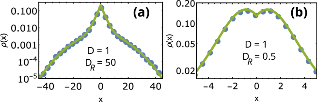
Figure 5: Variation in shapes of $\rho(x)$ for diffusion with stochastic returns modulated by harmonic potential is shown in comparison with the simulation data. We have considered two scenarios: (i) $D<D_{R}$ (panel a) – the slope near the origin is negative (see (38)) and (ii) $D<D_{R}$ (panel b) – the slope near the origin is positive (see (38)). Panel (a) shows a deviation from the linear behavior while the exponential tail appears at far away from the origin where the probability is small and hard to access by normal Monte-Carlo simulations. On the other hand, in panel (b), we see that $\rho(x)$ develops an exponential tail away from the origin. Parameters used here are: $k=0.3,~{}r=0.2$. Numerical simulations are performed for $dt=10^{-3}$ and $10^{6}$ realizations.

We now turn our attention to discuss the asymptotic behaviors of the steady state densities in the limits of small and large $x$ where again interesting observations can be made. In the small $x$ limit, expanding the total density around $x=0$, we get

$$\rho(x) \approx \frac{\alpha p_{M}}{2}\left[1+\alpha\left(\frac{D}{D_{R}}-1\right)|x|\right]+\frac{\alpha^{3}p_{M}}{4}\left[1-\frac{D}{D_{R}}\right]x^{2}$$ (38)

$$+ \frac{\alpha^{2}p_{M}}{12D_{R}^{2}}\left[\alpha^{2}DD_{R}-\alpha^{2}D_{R}^{2}-2kD\right]x^{2}|x|~{},$$

where we have used the following small $|x|$ asymptotic behaviour

$$\text{Erfi}\left[\frac{a-b|x|}{c}\right]\approx\text{Erfi}\left[\frac{a}{c}\right]-\frac{2b|x|}{c\sqrt{\pi}}~{}e^{a^{2}/c^{2}}~{}.$$ (39)

Note that when $D=D_{R}$, both the linear and second order terms in (38) drop out, thus the first and second order derivatives vanish at the origin. The leading contribution in this case comes from the third order term (see figure 4c). However, when $D_{R}\neq D$, we see the leading behavior (i.e., the slope) near the origin is determined by the linear term, and consequently one sees a deviation from the linear behavior (see figure 5). Various interesting shapes of the total density $\rho(x)$ are presented in figure 5.

We now proceed to perform the asymptotic analysis for large $x$. We first note that $\rho_{R}(x)$ in (36) can be written as a difference between two terms i.e., $\rho_{R}(x)=\rho_{R}^{I}(x)-\rho_{R}^{II}(x)$, where $\rho_{R}^{I(II)}(x)$ is the first (second) term on the RHS of (36). We find that for large $x$, $\rho_{R}^{II}(x)$ behaves asymptotically as

$$\rho_{R}^{II}(x) \approx \frac{rp_{M}}{2}\sqrt{\frac{\pi}{2\pi kD_{R}}}e^{-\frac{D_{R}\alpha^{2}}{2k}}e^{-\frac{kx^{2}}{2D_{R}}}\frac{\sqrt{2kD_{R}}}{\alpha D_{R}-k|x|}\exp\left[\left(\frac{-k|x|+\alpha D_{R}}{\sqrt{2kD_{R}}}\right)^{2}\right]$$ (40)

$$\approx \frac{\alpha p_{M}}{2}e^{-\alpha|x|}\frac{\alpha D}{\alpha D_{R}-k|x|}~{}.$$

Here note that $\rho_{R}^{I}(x)$ decays faster $(\sim e^{-x^{2}})$ than $\rho_{R}^{II}(x)$, hence can be neglected altogether. Combining all the individual contributions together, we find

$$\rho(x)\approx\frac{\alpha p_{M}}{2}e^{-\alpha|x|},$$ (41)

which again has an exponential tail in the large $|x|$ limit. We refer to figure 6 which shows a typical steady state distribution in this case exhibiting the linear behaviour at small $|x|$, then a crossover to an intermediate nonlinear behaviour before developing the exponential tail at large $|x|$.

5.3 $D_{R}\to 0$ limit

In this subsection, we discuss the $D_{R}\to 0$ limit which, in our case, makes the return protocols deterministic. In the first example of linear potential, this would mean that the particle is being pulled at a constant drift towards the resetting location. To see this, we take the limit in (27) to find $\rho_{R}(x)\approx\frac{rp_{M}}{2\lambda}e^{-\alpha|x|}$. Note that this result was already reported in [52] which was obtained by solving (19) with $D_{R}=0$. For the harmonic case, by taking $D_{R}\to 0$ limit in (36), we find $\rho_{R}(x)\approx\frac{rp_{M}}{2k|x|}e^{-\alpha|x|}$ where we have used the following asymptotic forms of the Erfi-function namely $\text{Erfi}[x\to 0]\approx\frac{2x}{\sqrt{\pi}}$ and $\text{Erfi}\left[|x|\to\infty\right]\approx\frac{1}{\sqrt{\pi}}\frac{e^{x^{2}}}{|x|}$. Again, this result can also be obtained by first putting $D_{R}=0$ in (19) and then solving $\frac{\partial}{\partial x}[kx\rho_{R}(x)]+\frac{r\alpha p_{M}}{2}e^{-\alpha|x|}=0$ with natural boundary conditions $\lim_{x\to\pm\infty}\rho_{R}(x)=0$. Note that the return density solutions obtained in this way take non-zero values when $x=0$. This is in contrast with the vanishing values obtained when evaluating the solutions (e.g., (27) and (36)) for $D_{R}\neq 0$, which is consistent with the boundary conditions in (9). Thus, we infer that the limits $x\to 0$ and $D_{R}\to 0$ do not commute and it may be related to the fact that the governing master equations in return phase (see e.g., (17)) change order in the sense that they become first order differential equations as derived for the deterministic return protocols [51, 52].

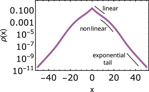
Figure 6: Behavior of the steady state density in the case of returns driven by harmonic potential $U(x)=\frac{1}{2}kx^{2}$ when $D\neq D_{R}$. We observe three different regimes in the steady state: linear (at small $x$), non-linear (intermediate) and an exponential tail (at large $x$). Parameters: $D=1,~{}D_{R}=12,~{}k=0.3,~{}r=0.2$.

6 Conclusions

In this paper, we have provided a formulation to study stochastic resetting processes which are subject to non-instantaneous returns. We have investigated the possibility of stochastic return protocols which were so far unexplored. We concur that in physical world microscopic processes are sensitive to thermal fluctuations and thus the return processes can also be random despite measurements with extreme precision. We have developed a comprehensive framework for such a set up which then systematically allows us to derive the governing equations for the observables like position herein, and potentially others in general.

In particular, our framework allows one to study the time evolution of the full process which can be decomposed into two stochastic phases. For each phase, we have derived Fokker Planck equations which are coupled through the probability currents to alternate between the phases. Utilizing our formalism, we then demonstrate how to capture the novel aspects of the position distributions especially in the steady state limit. Quite interestingly, we observed that some of the parameters emerged from the solutions can be interpreted in terms of the mean residence time in each phase.

It is important to emphasize that our approach is not only limited to diffusion in the phase I, but can easily be extended to a wide range of stochastic motions beyond diffusion (generated from an arbitrary Fokker-Plank operator $\mathcal{L}_{0}$). Furthermore, our formalism can readily be applied to settings with more general trapping potentials $U(x)$ other than linear or harmonic potential in phase II (see (6) and (7)). Thus, we believe that the framework put forward here offers a widespread applicability for the theory as well as future experimental studies of stochastic resetting.

Various generalizations of this problem can be immediately invited. While the thermodynamics of instantaneous resetting is only getting started [60, 61, 62, 63, 64], a future direction would be also to study thermodynamics of the models studied above. From the dynamical perspective, extreme statistics of resetting process has hardly been explored. It therefore remains to be seen how the extremal properties e.g., the statistics of largest excursion [65] will be ramified in the presence of resetting. Another interesting aspect would be to study the problem in the presence of an absorbing boundary or a target at a distance away from the resetting location. One could investigate the first passage properties such as the survival probability or the mean first passage time to the target in the presence of stochastic returns. Advantage can be taken by noting that the whole compound process gets renewed after each trial, and thus a renewal formalism applied to the full process seems to be a promising direction. In fact, if we assume that target detection is possible by the searcher only during motion phase, but not in return phase, one could apply the renewal structure as in stochastic resetting systems with refractory periods [26, 55] to obtain the first passage time statistics.

Remarkably, implementation of our resetting protocol does not require to track the particle during its return. A counter could be set which can detect when the particle makes a first passage to the origin. We refer to another recent study [66] that proposes similar ideas of diffusion with stochastic returns using intermittent resetting potentials.

7 Acknowledgements

D. G. is supported by “Excellence Project 2018” of the Cariparo foundation. C. A. P. acknowledges the support from University of Padova through Project No. STARS-Stg (CdA Rep. 40, 23.02.2018) BioReACT grant. A.K. acknowledges support from the SERB Early Career Research Award ECR/2017/000634 from the Science and Engineering Research Board, Department of Science and Technology and the support of the Department of Atomic Energy, Government of India, under project no. 12-R & D-TFR-5.10-1100. A.P. gratefully acknowledges Raymond and Beverly Sackler postdoctoral fellowship and Ratner Center for Single Molecule Science at the Tel Aviv University for funding.

Appendix A Mean first passage times of a Brownian particle in linear and quadratic potential

In this section, we present results for the mean first passage time in the context of our current problems. There are many standard ways to compute mean first passage time (see [67, 68, 69, 70, 71] for review and applications of the subject). Here, we adapt the approach of backward Fokker Planck equation which is often advantageous to treat the first passage properties [67, 68]. Within this context, we ask a simple question: given that a particle started its dynamics from the position $x$ at time zero, how much time $\tau(x)$ it will take to reach some threshold (in our case, the origin) for the first time. To compute the statistical properties of $\tau(x)$ it is convenient to consider the cumulative probability $Q(x,t)=\text{Prob.}[\tau(x)\geq t]$. Note that the probability $Q(x,t)$ is actually the survival probability that the particle, starting from $x$, survives from an absorbing boundary at the origin till time $t$. In other words, this is the probability that the particle does not hit the origin till time $t$. The first passage time density, denoted by $f_{\text{FP}}(\tau)$, is then given by $f_{\text{FP}}(\tau)=-\frac{\partial Q(x,\tau)}{\partial\tau}$. Hence the mean first passage time to the origin is given by

$$\overline{\tau}(x)=\int_{0}^{\infty}~{}dt~{}t\left[-\frac{\partial Q(x,t)}{\partial t}\right].$$ (42)

In the backward Fokker-Planck approach, one first considers the initial position as a variable, and then solves the backward equation with suitable boundary conditions self-consistently. The governing equation for the survival probability is given by [67, 68]

$$\frac{\partial Q(x,t)}{\partial t}=F(x)~{}\frac{\partial Q(x,t)}{\partial x}+D_{R}\frac{\partial^{2}Q(x,t)}{\partial x^{2}},$$ (43)

with the initial condition $Q(x,0)=1$ and the boundary conditions $Q(0,t)=0$. The Laplace transform $\tilde{Q}(x,s)=\int_{0}^{\infty}~{}dt~{}e^{-st}Q(x,t)$ of the survival probability then satisfies the following equation

$$-1+s\tilde{Q}(x,s)=D_{R}\frac{\partial^{2}\tilde{Q}(x,s)}{\partial x^{2}}+F(x)\frac{\partial\tilde{Q}(x,s)}{\partial x}.$$ (44)

It is easy to see that the boundary conditions mentioned above now gets modified to $\tilde{Q}(0,s)=0$ and moreover we used $\lim_{x\to\pm\infty}\tilde{Q}(x,s)<\infty$. Note from (42) that the mean first passage time can simply be obtained from the $s\to 0$ limit i.e.,

$$\overline{\tau}(x)=\tilde{Q}(x,s\to 0),$$ (45)

where the overline simply represents the average over the stochastic trajectories which start from a fixed position $x$ and we have assumed $\lim_{t\to\infty}tQ(x,t)=0$. However, in our problem we are required to perform an additional average over $x$, which we denote by $\langle\overline{\tau}(x)\rangle$. As discussed in the main text, this average is done over $\rho_{\text{inst}}(x)$.

Having sketched the basic steps, we are now ready to discuss the following two cases: (i) linear potential $U(x)=[\lambda_{+}\theta(x)+\lambda_{-}\theta(-x)]~{}|x|$, where $\lambda_{\pm}>0$ and (ii) harmonic potential $U(x)=\frac{1}{2}kx^{2}$ with $k>0$, as done in the main text.

A.1 $F(x)=\lambda_{-}\theta(-x)-\lambda_{+}\theta(x)$

We first consider linear potential case in which a Brownian particle which diffuses in a force field $F(x)=\lambda_{-}\theta(-x)-\lambda_{+}\theta(x)$. We want to compute the mean first passage time of this particle to the origin. Applying (44), we find

$$D_{R}\frac{\partial^{2}\tilde{Q}(x,s)}{\partial x^{2}}+\left[\lambda_{-}\theta(-x)-\lambda_{+}\theta(x)\right]\frac{\partial\tilde{Q}(x,s)}{\partial x}=-1+s\tilde{Q}(x,s)~{}.$$

Solving the above equations with the boundary conditions, we find

$$\tilde{Q}(x,s) = ~{}\frac{1}{s}\left[1-e^{-\frac{\sqrt{\lambda_{+}^{2}+4D_{R}s}-\lambda_{+}}{2D_{R}}x}\right],~{}x>0~{},$$

$$\tilde{Q}(x,s) = ~{}~{}\frac{1}{s}\left[1-e^{\frac{\sqrt{\lambda_{-}^{2}+4D_{R}s}-\lambda_{-}}{2D_{R}}x}\right],~{}x<0~{}.$$ (46)

Finally, utilizing (45) and substituting expressions for $\tilde{Q}(x,s)$ from (46) we arrive at the following expression for the mean first passage time

$$\overline{\tau}(x)=|x|\left[\frac{\theta(x)}{\lambda_{+}}+\frac{\theta(-x)}{\lambda_{-}}\right]~{},$$ (47)

which was used in section 5.1 to compute the mean return time. Finally substituting the above expression in (22) with the use of (24), we get

$$\langle\overline{\tau}(x)\rangle=\int\limits_{-\infty}^{\infty}~{}dx~{}\overline{\tau}(x)\left[\frac{\alpha}{2}e^{-\alpha|x|}\right]=\frac{1}{2\alpha}\left(\frac{1}{\lambda_{+}}+\frac{1}{\lambda_{-}}\right)~{},$$ (48)

which was announced in the main text (see section 5.1).

A.2 $F(x)=-kx$

In this section, we move on to compute the mean first passage time of a Brownian particle diffusing in a potential $U(x)=\frac{1}{2}kx^{2}$. We again start with the Laplace space backward Fokker-Planck equation for the survival probability

$$D_{R}\frac{\partial^{2}\tilde{Q}(x,s)}{\partial x^{2}}-kx\frac{\partial\tilde{Q}(x,s)}{\partial x}=-1+s\tilde{Q}(x,s)~{},$$ (49)

with the boundary conditions $\tilde{Q}(0,s)=0$ and $\lim_{x\to\pm\infty}\tilde{Q}(x,s)<\infty$. First we take out the homogeneous part by redefining: $y(x,s)=\tilde{Q}(x,s)-\frac{1}{s}$. This gives us

$$\frac{d^{2}y}{dx^{2}}-\gamma_{R}x\frac{dy}{dx}-\frac{s}{D_{R}}y=0~{},$$ (50)

where $\gamma_{R}=k/D_{R}$. Let’s now do the following change of variable:

$$x=\sqrt{\frac{\xi}{\gamma_{R}}}~{},~{}~{}~{}y(x(\xi))=w(\xi)~{}.$$ (51)

This gives us

$$\xi\frac{d^{2}w}{d\xi^{2}}+\frac{1}{2}(1-\xi)\frac{dw}{d\xi}-aw=0~{}~{},~{}~{}~{}a=\frac{s}{4k}~{}.$$ (52)

Getting solutions for the above equation from [58, 59] and reverting back to $y(x,s)$ we finally arrive at

$$y(x,s)=c_{1}x\sqrt{\gamma_{R}}~{}\mathcal{U}\left(\frac{1+4a}{2},\frac{3}{2},\frac{\gamma_{R}x^{2}}{2}\right)~{},~{}x>0~{},$$ (53)

where we have imposed the boundary condition $y(x\to\infty,s)<\infty$. Note that here $\mathcal{U}(a,b,z)$ is the Tricomi confluent hypergeometric function [58, 59]. Further noting that $y(0,s)=-1/s$, we find

$$c_{1}~{}\frac{\sqrt{2\pi}}{\Gamma(\frac{1}{2}+2a)}=-1/s,~{}~{}x>0~{},$$ (54)

where $\Gamma(z)$ is the Gamma function. Thus the solution for the survival probability in the positive $x$-axis reads

$$\tilde{Q}^{+}(x,s)=\frac{1}{s}\left[1-\frac{\Gamma(\frac{1}{2}+2a)}{\sqrt{2\pi}}x\sqrt{\gamma_{R}}~{}\mathcal{U}\left(\frac{1+4a}{2},\frac{3}{2},\frac{\gamma_{R}x^{2}}{2}\right)\right].$$

Since the solution is symmetric around zero, we have $\tilde{Q}^{-}(x,s)=\tilde{Q}^{+}(-x,s)$. Using the above expressions for the survival probability and substituting in (45), we arrive at the following expression for the mean first passage time

$$\overline{\tau}(x)=-\frac{\mathcal{U}^{(1,0,0)}\left(0,\frac{1}{2},\frac{\gamma_{R}x^{2}}{2}\right)+\psi^{(0)}\left(\frac{1}{2}\right)}{2D_{R}\gamma_{R}}>0,\hskip 14.22636pt$$ (56)

where $\mathcal{U}^{(1,0,0)}(a,b,z)$ is the partial derivative of the Tricomi confluent hypergeometric function $\mathcal{U}(a,b,z)$ with respect to $a$ and $\psi^{(0)}(z)$ is the digamma function defined as the logarithmic derivative of the gamma function i.e., $\psi^{(0)}(z)=\Gamma^{\prime}(z)/\Gamma(z)$ [58, 59]. In particular, one finds $\psi^{(0)}(\frac{1}{2})=-(\gamma+\ln{4})=-1.9635$, where $\gamma$ is the Euler’s constant. Substituting this into (56) gives us the solution for the mean first passage time to the origin (i.e., (37)) for a Brownian particle diffusing in a harmonic potential given that it had started from $x$. Now averaging $x$ over the steady state density $\rho_{\text{inst}}(x)$, we find the mean return time $\langle\overline{\tau}(x)\rangle=\int~{}dx~{}\overline{\tau}(x)\rho_{\text{inst}}(x)$ (recall (22)). Note that, the latter integral can not be computed exactly. Hence we evaluate the integral numerically.

Appendix B Method of numerical simulation

In the following, we outline the method that is used to numerically simulate our set up (see Sec. 2). In particular, we consider that in phase-I, the particle performs a simple diffusion. Upon resetting, the particle returns under the action of force $F(x)$ generated by the potential $U(x)$ centered at the resetting location. To obtain the distribution of the position of the particle at time $t$, we discretize the time $t=n~{}dt$, where $n$ is an integer. We initialize the position of the particle in the diffusion phase $x(0)=0$, and then, for the first interval $i=1$, the particle evolves under the following discrete version of the Langevin dynamics

$$x(dt)=x(0)+\sqrt{2~{}D~{}dt}~{}\eta,$$ (57)

where $\eta$ is the Gaussian random variable with mean $0$ and variance $1$, and $dt$ is the microscopic time step. The evolution in the remaining steps is as follows. In the next step ($i=2$), the particle can either reset or it can keep evolving. Thus,

1. with probability $1-r~{}dt$ ($r$ is the rate of resetting), the particle still undergoes diffusion so that

   $$x(i~{}dt)=x((i-1)~{}dt)+\sqrt{2~{}D~{}dt}~{}\eta,$$ (58)

2. whereas with complementary probability $r~{}dt$, resetting occurs, and the return phase resumes. Herein, the particle diffuses in a potential $U(x)$ centered at the resetting location (the origin). The discreteized version of the dynamics in the return phase then reads

   $$x(i~{}dt)=x((i-1)~{}dt)-U^{\prime}[x(i~{}dt)]dt+\sqrt{2~{}D_{R}~{}dt}~{}\eta.$$ (59)

The dynamics governed by (59) continues until it hits the minimum of the potential for the first time. In other words, we stop the return phase dynamics when for the first time $x(t)$ changes sign. The particle now reenters the diffusive phase, and we proceed as outlined above until $i=n$. We record the position of the particle as a function of observation time for $\mathcal{N}_{R}$ number of independent realizations. Finally, we construct the histogram of the position of the particle averaged over these realizations.

References

- [1] Evans, M.R. and Majumdar, S.N., 2011. Diffusion with stochastic resetting. Physical review letters, 106(16), p.160601.
- [2] Evans, M.R. and Majumdar, S.N., 2011. Diffusion with optimal resetting. Journal of Physics A: Mathematical and Theoretical, 44(43), p.435001.
- [3] Evans, M.R., Majumdar, S.N. and Mallick, K., 2013. Optimal diffusive search: nonequilibrium resetting versus equilibrium dynamics. Journal of Physics A: Mathematical and Theoretical, 46(18), p.185001.
- [4] Majumdar, S.N., Sabhapandit, S. and Schehr, G., 2015. Dynamical transition in the temporal relaxation of stochastic processes under resetting. Physical Review E, 91(5), p.052131.
- [5] Eule, S. and Metzger, J.J., 2016. Non-equilibrium steady states of stochastic processes with intermittent resetting. New Journal of Physics, 18(3), p.033006.
- [6] Durang, X., Henkel, M. and Park, H., 2014. The statistical mechanics of the coagulation–diffusion process with a stochastic reset. Journal of Physics A: Mathematical and Theoretical, 47(4), p.045002.
- [7] Pal, A., 2015. Diffusion in a potential landscape with stochastic resetting. Physical Review E, 91(1), p.012113.
- [8] Pal, A., Kundu, A. and Evans, M.R., 2016. Diffusion under time-dependent resetting. Journal of Physics A: Mathematical and Theoretical, 49(22), p.225001.
- [9] Pal, A. and Prasad, V.V., 2019. First passage under stochastic resetting in an interval. Physical Review E, 99(3), p.032123.
- [10] Méndez, V. and Campos, D., 2016. Characterization of stationary states in random walks with stochastic resetting. Physical Review E, 93(2), p.022106.
- [11] Gupta, D., 2019. Stochastic resetting in underdamped Brownian motion. Journal of Statistical Mechanics: Theory and Experiment, 2019(3), p.033212.
- [12] Pal, A., Chatterjee, R., Reuveni, S. and Kundu, A., 2019. Local time of diffusion with stochastic resetting. Journal of Physics A: Mathematical and Theoretical, 52(26), p.264002.
- [13] Meylahn, J.M., Sabhapandit, S. and Touchette, H., 2015. Large deviations for Markov processes with resetting. Physical Review E, 92(6), p.062148.
- [14] Abdoli, I., Vuijk, H.D., Wittmann, R., Sommer, J.U., Brader, J.M. and Sharma, A., 2020. Novel stationary state in Brownian systems with Lorentz force. arXiv preprint arXiv:2004.04471.
- [15] Plata, C.A., Gupta, D. and Azaele, S., 2020. Asymmetric Stochastic Resetting: Modeling Catastrophic Events. arXiv preprint arXiv:2007.12417.
- [16] Reuveni, S., Urbakh, M. and Klafter, J., 2014. Role of substrate unbinding in Michaelis–Menten enzymatic reactions. Proceedings of the National Academy of Sciences, 111(12), pp.4391-4396.
- [17] Rotbart, T., Reuveni, S. and Urbakh, M., 2015. Michaelis-Menten reaction scheme as a unified approach towards the optimal restart problem. Physical Review E, 92(6), p.060101.
- [18] Roldan, E., Lisica, A., Sanchez-Taltavull, D. and Grill, S.W., 2016. Stochastic resetting in backtrack recovery by RNA polymerases. Physical Review E, 93(6), p.062411.
- [19] Evans, M.R. and Majumdar, S.N., 2018. Run and tumble particle under resetting: a renewal approach. Journal of Physics A: Mathematical and Theoretical, 51(47), p.475003.
- [20] Luby, M., Sinclair, A. and Zuckerman, D., 1993. Optimal speedup of Las Vegas algorithms. Information Processing Letters, 47(4), pp.173-180.
- [21] Montanari, A. and Zecchina, R., 2002. Optimizing searches via rare events. Physical review letters, 88(17), p.178701.
- [22] Kusmierz, L., Majumdar, S.N., Sabhapandit, S. and Schehr, G., 2014. First order transition for the optimal search time of Lévy flights with resetting. Physical review letters, 113(22), p.220602.
- [23] Bressloff, P.C., 2020. Directed intermittent search with stochastic resetting. Journal of Physics A: Mathematical and Theoretical, 53(10), p.105001.
- [24] Falcon-Cortes, A., Boyer, D., Giuggioli, L. and Majumdar, S.N., 2017. Localization transition induced by learning in random searches. Physical review letters, 119(14), p.140603.
- [25] Chechkin, A. and Sokolov, I.M., 2018. Random search with resetting: a unified renewal approach. Physical review letters, 121(5), p.050601.
- [26] Pal, A., Kuśmierz, Ł and Reuveni, S., 2019. Home-range search provides advantage under high uncertainty. arXiv preprint arXiv:1906.06987.
- [27] Pal, A., Kuśmierz, Ł and Reuveni, S., 2019. Invariants of motion with stochastic resetting and space-time coupled returns, New J. Phys. 21 113024
- [28] Evans, M.R., Majumdar, S.N. and Schehr, G., 2020. Stochastic resetting and applications. Journal of Physics A: Mathematical and Theoretical.
- [29] Tal-Friedman, O., Pal, A., Sekhon, A., Reuveni, S. and Roichman, Y., 2020. Experimental realization of diffusion with stochastic resetting. J. Phys. Chem. Lett. 2020, 11, 17, 7350–7355
- [30] Besga, B., Bovon, A., Petrosyan, A., Majumdar, S. and Ciliberto, S., 2020. Optimal mean first-passage time for a Brownian searcher subjected to resetting: experimental and theoretical results. Phys. Rev. Research 2, 032029(R) (2020).
- [31] Masoliver, J. and Montero, M., 2019. Anomalous diffusion under stochastic resettings: A general approach. Physical Review E, 100(4), p.042103.
- [32] Maso-Puigdellosas, A., Campos, D. and Mendez, V., 2019. Anomalous diffusion in random-walks with memory-induced relocations. Frontiers in Physics, 7, p.112.
- [33] dos Santos, M.A., 2019. Fractional Prabhakar derivative in diffusion equation with non-static stochastic resetting. Physics, 1(1), pp.40-58.
- [34] Bodrova, A.S., Chechkin, A.V. and Sokolov, I.M., 2019. Nonrenewal resetting of scaled Brownian motion. Physical Review E, 100(1), p.012119.
- [35] Shkilev, V.P., 2017. Continuous-time random walk under time-dependent resetting. Physical Review E, 96(1), p.012126.
- [36] Kusmierz, L.. and Gudowska-Nowak, E., 2019. Subdiffusive continuous-time random walks with stochastic resetting. Physical Review E, 99(5), p.052116.
- [37] Kusmierz, L. and Gudowska-Nowak, E., 2015. Optimal first-arrival times in Lévy flights with resetting. Physical Review E, 92(5), p.052127.
- [38] Gupta, S., Majumdar, S.N. and Schehr, G., 2014. Fluctuating interfaces subject to stochastic resetting. Physical review letters, 112(22), p.220601.
- [39] Basu, U., Kundu, A. and Pal, A., 2019. Symmetric exclusion process under stochastic resetting. Physical Review E, 100(3), p.032136.
- [40] Karthika, S. and Nagar, A., 2020. Totally asymmetric simple exclusion process with resetting. Journal of Physics A: Mathematical and Theoretical, 53(11), p.115003.
- [41] Sadekar, O. and Basu, U., 2020. Zero-current Nonequilibrium State in Symmetric Exclusion Process with Dichotomous Stochastic Resetting. J. Stat. Mech. 073209.
- [42] Reuveni, S., 2016. Optimal stochastic restart renders fluctuations in first passage times universal. Physical review letters, 116(17), p.170601.
- [43] Pal, A. and Reuveni, S., 2017. First Passage under Restart. Physical review letters, 118(3), p.030603.
- [44] Pal, A., Eliazar, I. and Reuveni, S., 2019. First passage under restart with branching. Physical review letters, 122(2), p.020602.
- [45] Belan, S., 2018. Restart could optimize the probability of success in a Bernoulli trial. Physical review letters, 120(8), p.080601.
- [46] Pal, A. and Prasad, V.V., 2019. Landau-like expansion for phase transitions in stochastic resetting. Physical Review Research, 1(3), p.032001.
- [47] Ray, S., Mondal, D. and Reuveni, S., 2019. Peclet number governs transition to acceleratory restart in drift-diffusion. Journal of Physics A: Mathematical and Theoretical, 52(25), p.255002.
- [48] Nagar, A. and Gupta, S., 2016. Diffusion with stochastic resetting at power-law times. Physical Review E, 93(6), p.060102.
- [49] Ray, S. and Reuveni, S., 2020. Diffusion with resetting in a logarithmic potential. J. Chem. Phys. 152, 234110.
- [50] Ahmad, S., Nayak, I., Bansal, A., Nandi, A. and Das, D., 2019. First passage of a particle in a potential under stochastic resetting: A vanishing transition of optimal resetting rate. Physical Review E, 99(2), p.022130.
- [51] Pal, A., Kuśmierz, Ł and Reuveni, S., 2019. Invariants of motion with stochastic resetting and space-time coupled returns. New Journal of Physics, 21(11), p.113024.
- [52] Pal, A., Kuśmierz, Ł and Reuveni, S., 2019. Time-dependent density of diffusion with stochastic resetting is invariant to return speed. Physical Review E, 100(4), p.040101.
- [53] Bodrova, A.S. and Sokolov, I.M., 2019. Resetting processes with noninstantaneous return. Physical Review E, 101(5), p.052130.
- [54] Maso-Puigdellosas, A., Campos, D. and Mendez, V., 2019. Transport properties of random walks under stochastic noninstantaneous resetting. Physical Review E, 100(4), p.042104.
- [55] Evans, M.R. and Majumdar, S.N., 2018. Effects of refractory period on stochastic resetting. Journal of Physics A: Mathematical and Theoretical, 52(1), p.01LT01.
- [56] Neuman, K.C. and Block, S.M., 2004. Optical trapping. Review of scientific instruments, 75(9), pp.2787-2809.
- [57] Frank Jülicher, Armand Ajdari, and Jacques Prost, (1997). Modeling molecular motors, Rev. Mod. Phys. 69, 1269.
- [58] Zaitsev, V.F. and Polyanin, A.D., 2002. Handbook of exact solutions for ordinary differential equations. CRC press.
- [59] Olver, F.W., Lozier, D.W., Boisvert, R.F. and Clark, C.W. eds., 2010. NIST handbook of mathematical functions hardback and CD-ROM. Cambridge university press.
- [60] Fuchs, J., Goldt, S. and Seifert, U., 2016. Stochastic thermodynamics of resetting. EPL (Europhysics Letters), 113(6), p.60009.
- [61] Pal, A. and Rahav, S., 2017. Integral fluctuation theorems for stochastic resetting systems. Physical Review E, 96(6), p.062135.
- [62] Gupta, D., Plata, C.A. and Pal, A., 2020. Work fluctuations and Jarzynski equality in stochastic resetting. Physical Review Letters, 124(11), p.110608.
- [63] Busiello, D.M., Gupta, D. and Maritan, A., 2020. Entropy production in systems with unidirectional transitions. Physical Review Research, 2(2), p.023011.
- [64] Pal, A., Reuveni, S. and Rahav, S., 2020. Thermodynamic uncertainty relation for systems with unidirectional transitions. arXiv preprint arXiv:2008.06953.
- [65] Majumdar, S.N., Pal, A. and Schehr, G., 2019. Extreme value statistics of correlated random variables: a pedagogical review. Physics Reports, 840, pp.1-32.
- [66] Mercado-Vásquez, G., Boyer, D., Majumdar, S.N. and Schehr, G., 2020. Intermittent resetting potentials. arXiv preprint arXiv:2007.15696.
- [67] Redner, S., 2007. A Guide to First-Passage Processes. A Guide to First-Passage Processes, by Sidney Redner, Cambridge, UK: Cambridge University Press, 2007.
- [68] Bray, A.J., Majumdar, S.N. and Schehr, G., 2013. Persistence and first-passage properties in nonequilibrium systems. Advances in Physics, 62(3), pp.225-361.
- [69] Metzler, R., Oshanin, G. and Redner, S. eds., 2014. First-passage phenomena and their applications. World Scientific Publishing.
- [70] Grebenkov, D.S., 2014. First exit times of harmonically trapped particles: a didactic review. Journal of Physics A: Mathematical and Theoretical, 48(1), p.013001.
- [71] Benichou, O., Loverdo, C., Moreau, M. and Voituriez, R., 2011. Intermittent search strategies. Reviews of Modern Physics, 83(1), p.81.