Inferring epidemic parameters for COVID-19 from fatality counts in Mumbai

Abstract

Epidemic parameters are estimated through Bayesian inference using the daily fatality counts in Mumbai during the period from March 31 to April 14. A doubling time of 5.5 days (median with $[4.6,6.9]$ days 95% CrI) is observed. In the SEIR model this gives the basic reproduction rate $R_{0}$ of 3.4 (median with $[2.4,4.8]$ 95% CrI). Using as input the infection fatality rate and the interval between infection and death, the number of infections in Mumbai is inferred. It is found that the ratio of the number of test positives to the total infections is 0.13% (median), implying that tests are currently finding 1 out of 750 cases of infection. After correcting for different testing rates, this result is compatible with a measurement of the ratio made recently via serological testing in the USA. From the estimates of the number of infections we infer that the first COVID-19 cases were seeded in Mumbai between late December 2019 and early February 2020. provided the doubling times remained unchanged since then. We remark on some public health implications if the rate of growth cannot be controlled in about a week.

TIFR/TH/20-11

I Introduction

In many countries across the world, there is an initial bottleneck in testing for COVID-19. This is due to a combination of two factors, first the availability of test kits, and second, of trained laboratory personnel to perform the tests. When the number of tests per million of population is limited, the exponential growth in infections at the beginning of an epidemic makes it impossible to estimate the prevalence of infections in any meaningful way. One aim of this paper is to establish and validate a Bayesian statistical inference procedure to make a probabilistic estimate of the infected population from the statistics of fatalities. This is done using data for Mumbai, which is one of the major COVID-19 epidemic hot spots in India.

The counts of fatalities due to COVID-19 also have errors. The most important is the fraction of mis-diagnosis. At the current time, it is unlikely that a patient who dies of severe acute respiratory illness (SARI) will be misdiagnosed. We know that the Municipal Corporation of Greater Mumbai (MCGM) tries to track, and report on, every such case, even if the diagnosis comes a few days after the fatality. Another source of systematic error in the count of fatalities may come from a part of the population with limited access to health care. This is not a trivial source of error, and corporations have to check their death records very thoroughly to make sure that no case is missed. In New York City, where the number of daily fatalities attributed to COVID-19 has been more than 100 since late March nychealth the local government is wary of undercounts reuters . Similar undercounts have been reported from several European countries forbes , and a correction by 100–200% was found to be necessary. A retrospective correction in the record of fatalities is being carried out in Wuhan. Nevertheless, fatality counts may be in error by a factor 2–3, whereas testing could potentially have errors which are one or two orders of magnitude higher.

In view of this, it makes sense to estimate epidemic parameters from the daily count of fatalities, $D(t)$, rather than less uncertain statistics such as the daily count of test positives $T_{+}(t)$. This is the primary aim of this paper. Daily fatality counts in Mumbai are currently less than 20. This is about one part in a million of the population, and an order of magnitude below peak rates in cities of comparable size elsewhere in the world. The simplifying assumption that the epidemic is still in the stage of exponential growth is then viable. The exponential growth rate can then be reliably extracted from $D(t)$ without using any detailed model. Detailed analysis of the data also allows validation of this assumption, as we discuss in the results section of this paper.

Two more parameters, the infection fatality rate, ${\rm IFR\/}$, and the interval from infection to death, $T$, relate the number of infections, $I(t)$, and $D(t)$. Since data on $I(t)$ in Mumbai are currently unreliable, these two parameters are taken from the literature ifr to predict a credible interval for $I(t)$. Alternative estimates of $I(t)$ would, of course, constrain these parameters. First reports of such alternative estimates are now available from other locations seroprev . We find that the ratio $\Pi=T_{+}(t)/I(t)$ is small, and has been almost independent of time in Mumbai. This ratio has also been reported in seroprev . It is checked that the estimate of $\Pi$ made here is compatible with that, provided that the different testing rates in different countries are taken into account.

These statistical inferences lead directly to estimates of the date at which the initial seeding of COVID-19 took place. The further assumption which goes into this estimate is that the growth rate has remained unchanged. Another caveat should be kept in mind. Due to the statistical nature of infections, it is possible that multiple seedings occurred, and that the date obtained by the procedure followed here gives an average over such statistics. Stochastic models would refine our understanding of the early growth process. Genomic studies of multiple samples of the virus yadav in Mumbai would be independent data which could constrain such models.

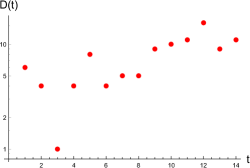
Figure 1: The number of daily fatalities due to COVID-19 in Mumbai on every day in April up to April 14. More recent data has not been analyzed together with this, because retrospective corrections may be applied for those. Notice the log scale on the $y$-axis.

MCGM releases a daily count of fatalities due to COVID-19, and performs retrospective corrections due to late receipt of test results or other post-mortem analysis. Due to this, the count of fatalities may take a few days to settle down. Changes in municipal priorities may also affect resources assigned to various tasks, resulting in systematic changes in the statistical character of data streams. Any analysis of epidemic parameters must allow for checks of such confounding factors. Other data streams, such as the municipal records of deaths, are harder to access. However, such records will need to be subjected to statistical analysis later to ascertain whether there were possible cryptic fatalities due to COVID-19. The methods used here can also be utilized to analyze the results of such an appraisal.

II Method

II.1 Data used

Daily counts released by MCGM have been archived prahlad . Here the summed and anonymous data on fatalities is analyzed for the two-week period between May 30 and April 14. The basic data on counts is displayed in Figure 1. No clear trend can be distinguished in the first week, but a clear exponential growth, characteristic of the early stages of epidemics, can be seen in the second week.

II.2 Mathematical formulation: estimation of doubling time

During the early stages of an epidemic the number of fatalities is expected to grow exponentially, doubling in every $\tau$ days,

$$D(t)={\cal D}_{0}2^{t/\tau}.$$ (1)

The parameter ${\cal D}_{0}$ is an estimate of the number of fatalities at the time when the counting starts. Both $\tau$ and ${\cal D}_{0}$ will be treated as parameters to be determined from the time series $D(t)$ using a standard Bayesian inference process.

Given the set of parameters $\pi=\{\tau,{\cal D}_{0}\}$, and the set of data to be fitted $\{D_{1},D_{2},\cdots\}$, which are the fatalities on days 1, 2, etc., and the errors $\{\sigma_{1},\sigma_{2},\cdots\}$, the probability distribution function (PDF) of $D_{i}$ given $\pi$ is defined as

$$P(D_{1},D_{2},\cdots|\pi)=\exp\left[-\sum_{t}\frac{[D_{t}-D(t)]^{2}}{\sigma_{t}^{2}}\right]$$ (2)

where $D(t)$ is the model of eq. (1), which depends on $\pi$. With the present disease surveillance regime, significant miscounts of $D_{t}$ would come only from small clusters of unnoticed infections, which would grow at roughly the same rate as the rest of the population. So the error would be a fraction of $D_{t}$. We will take $\sigma_{t}=fD_{t}$, with two scenarios of $f$. In scenario L, the low error scenario, we take $f=0.1$, i.e., assume 10% errors on $D_{t}$. In scenario M, the medium error scenario, we double the errors and take $f=0.2$. Bayes’ theorem can be used to write the posterior PDF for $\pi$,

$$P(\pi|D_{1},D_{2},\cdots)\propto P(D_{1},D_{2},\cdots|\pi)P_{0}(\pi)$$ (3)

where $P_{0}(\pi)$ is called the prior PDF of the parameters The constant of proportionality, which is the prior PDF of the data, is trivial, since it does not depend on $\pi$, and serves only to normalize the posterior PDF. Maximizing the posterior PDF gives the best values of $\pi$. We will also quote the 95% credible intervals (95% CrI) obtained from the posterior distribution.

The prior PDF is taken to be the product of two independent Gamma distributions, one for each of the parameters, $p_{0}({\cal D}_{0})=\Gamma({\cal D}_{0};k_{0},\theta_{0})$ and $p_{0}(\tau)=\Gamma(\tau;k,\theta)$. We take the meta-parameter $\theta=\theta_{0}=10$, so that we don’t suffer from overconfidence in priors lahiri . The parameters $k$ and $k_{0}$ are chosen to give the most probable prior values of $\tau=10$ days and ${\cal D}_{0}=5$. It was checked that different choices of prior parameters gave results which were insensitive to the choices.

II.3 Mathematical formulation: estimation of number of infections

$I_{0}$, the number of infections on day zero, can be inferred from ${\cal D}_{0}$ by a straightforward argument previous . First, the infection fatality rate, ${\rm IFR\/}$, gives a statistical estimate of the number of infections, ${\cal I\/}$, which resulted in the observed fatalities on day zero. This is simply ${\cal I\/}={\cal D}_{0}/{\rm IFR\/}$. The value of ${\rm IFR\/}$ could change from country to country because of differing age and gender structure of populations, or due to prevailing health conditions. However, a larger source of uncertainty is in the fraction of asymptomatic cases. As a result, ${\rm IFR\/}$ estimates vary from over 1% russell to under 0.5% cebm . Based on an complete sampling of a well-defined population, it has been estimated that the age and gender averaged ${\rm IFR\/}$ is 0.657% ifr . This is the estimate that we use here. A recent preprint goli updates the work in previous by correcting this value using Indian census data to obtain a value which is approximately two thirds of this. Using this number would boost our median estimates by about 50%. Since the 95% CrI are much larger, we do not incorporate this correction.

From ${\cal I\/}$ it is possible to construct $I_{0}$ using the previous estimate of $\tau$ to write $I_{0}=2^{T/\tau}{\cal I\/}$. Also, $T=t_{1}+t_{2}$ where $t_{1}$ is the incubation period, i.e., the interval between infection and the occurrence of symptoms, and $t_{2}$ is the interval between the occurrence of symptoms and death. Several independent estimates agree that the median value of $t_{1}$ is around 5 days lauer ; li . For $t_{2}$ we use the mean of 18.8 days and coefficient of variation of 0.25 ifr .

Putting these together we have

$$I_{0}={\cal D}_{0}\left[\frac{1}{{\rm IFR\/}}\times 2^{T/\tau}\right],\qquad{\rm with}\qquad T=t_{1}+t_{2},$$ (4)

and the distributions of the three parameters are taken to be $\Gamma({\rm IFR\/};6.3,0.0011)$, $\Gamma(t_{1};2.06,2.93)$ and $\Gamma(t_{2};16,1.175)$. The amplification factor, within square brackets, has all the uncertainties associated with these inputs, unlike the parameters ${\cal D}_{0}$ and $\tau$. Nevertheless, $I_{0}$ is of high interest for public health reasons, so we will present estimates.

III Results

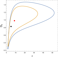
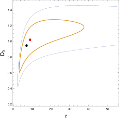
Figure 2: The best fit values of $\tau$ and ${\cal D}_{0}$ assuming 20% errors on the number of fatalities using the data between March 31 and April 4. The panel on the left is for Scenario M and that on the right for Scenario L. The best fit (modal values) given in eq. (5) are denoted by the black dots, and the medians by the red dots. The inner curve encloses the 95% CrI, and the outer curve the 99% CrI (for Scenario M) or the 97% CrI (for Scenario L) for which the 99% CrI curve is very far away on this scale.

III.1 March 31 to April 4

The first analysis was performed with the short time series for fatalities between March 31 and April 4. The most likely model that emerges out of the data is

$${\rm Scenario\ M:\/} \quad\tau=5.0{\rm\ days},\quad{\cal D}_{0}=0.83,\quad{\rm which\ implies}\quad I_{0}=17000\;[2000,350000]\;95\%{\rm\ CrI\/}.$$

$${\rm Scenario\ L:\/} \quad\tau=7.1{\rm\ days},\quad{\cal D}_{0}=0.95,\quad{\rm which\ implies}\quad I_{0}=\phantom{0}4600\;[\phantom{0}900,\phantom{0}42000]\;95\%{\rm\ CrI\/}.$$ (5)

The joint 95% and 99% CrI on the model parameters are shown in Figure 2. Note that the posterior distribution of the model parameters is strongly non-Gaussian. From the posterior PDF for $\tau$, marginalized over ${\cal D}_{0}$ in scenario M, we find $\tau$ to be 8.75 days (median values) and $[3.2,30]$ days 95% CrI, giving a significant probability of very long doubling times. From the PDF for ${\cal D}_{0}$, marginalized over $\tau$, we find a median of 0.98 and $[0.6,1.3]$ 95% CrI. One sees in Figure 2 that there is a broad tail to the posterior PDF which allows slightly larger values of ${\cal D}_{0}$ to compensate for a much slower epidemic growth. Longer time series are needed to rule this out, as will be seen later.

In Scenario L, after marginalizing over ${\cal D}_{0}$, $\tau$ is found to be 9.0 days (median) with $[4.8,27]$ days 95% CrI. For ${\cal D}_{0}$ it was seen that ${\cal D}_{0}=1.02$ and $[0.8,1.2]$ 95% CrI. The wide difference between the 95% CrI and the 99% CrI curves in scenario L is an indication that 10% Gaussian errors in scenario L are unable to give a good description of the jitter in the time series. In view of this, scenario L is not used in subsequent analyses.

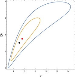
Figure 3: The best fit values of $\tau$ and ${\cal D}_{0}$ (day zero chosen to be April 2) in Scenario M using data between April 6 and 14. The best fit (modal values) is denoted by the black dot, and the median by the red dot. The inner curve encloses the 95% CrI, and the outer one the 99% CrI.

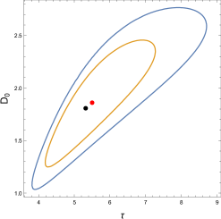
Figure 4: The best fit values of $\tau$ and ${\cal D}_{0}$ (on March 30) using the data set between March 31 and April 14, corrected for the change in intensity of surveillance soon after April 2, as described in the text. The best fit (modal values) is denoted by the black dot, and the median by the red dot. The inner curve encloses the 95% CrI, and the outer one the 99% CrI.

III.2 April 6 to April 14

The second part of the analysis used the data for the eight days between April 6 and 14, with day zero to be April 2. So ${\cal D}_{0}$ and $I_{0}$ in this context are estimates of the inferred number of infected cases in Mumbai on April 2. Note that this time series is almost 50% longer than the first, and therefore regulates some of the peculiarities seen earlier. The most likely model parameters in Scenario M are

$$\tau=5.1{\rm\ days},\quad{\cal D}_{0}=2.5,\quad{\rm which\ implies}\quad I_{0}=44000\;[5500,960000]\;95\%{\rm\ CrI\/}.$$ (6)

The 95% and 99% CrI on the joint distribution of model parameters are shown in Figure 3. Although the contours are not as distorted as in Figure 2, they are clearly not ellipses. So the posterior PDF is distinctly non-Gaussian. After marginalizing over ${\cal D}_{0}$, we find $\tau$ is 5.6 days (median) and $[4.1,8.4]$ days 95% CrI. This 95% CrI is fully contained in the 95% CrI of $\tau$ for the earlier data set, showing that the estimates are totally compatible. For ${\cal D}_{0}$ we find, after marginalizing the posterior PDF over $\tau$, 2.75 (median) and $[1.8,4]$ 95% CrI.

Given the range of $\tau$ quoted above, in 3 days between March 31 and April 2, one expects ${\cal D}_{0}$ on May 31 to increase by a factor $[1.3,1.7]$ 95% CrI, and become $[1.0,2.0]$ 95% CrI. While this interval overlaps with that quoted above, the probability that the two estimates are statistically indistinguishable is about 3.8%. The reason for this discrepancy can be traced to a change in the surveillance policy instituted on April 2 news . The increased vigilance after this date must be corrected for in order to compare the two data sets. One can account for this by changing the overall normalization of the earlier data set by a factor of 1.7. This then increases the probability of agreement between the two analyses by an order of magnitude.

If one restricts the time series between April 6 and 12, one sees “by eye” that there could be rapid exponential growth. For this specially selected data set, we find that the most probable $\tau$ is 2.8 days. There is only a 20% probability that $\tau$ is as large as 4 days or more. These alarming results are biased. It is important to remember that infection spreading is a stochastic process, and there are always short runs of low or high growth.

III.3 The full set March 31 to April 14

Third, the analysis of the full data set is presented. A reporting discrepancy between the series up to April 4 and the later part was discussed in the previous section. We applied the correction developed there, and rounded $D(t)$ to the nearest integer. This corrected time series gave

$$\tau=5.3{\rm\ days},\quad{\cal D}_{0}=1.8,\quad{\rm which\ implies}\quad I_{0}=27000\;[3500,520000]\;95\%{\rm\ CrI\/}.$$ (7)

The 95% CrI of the joint distribution is shown in Figure 4. The PDF for $\tau$ marginalized over ${\cal D}_{0}$ gives $\tau=5.5$ days (median) with $[4.6,6.9]$ days 95% CrI, and that for ${\cal D}_{0}$ marginalized over $\tau$ gives ${\cal D}_{0}=1.86$ (median) with $[1.45,2.35]$ 9̧5. These are our primary results.

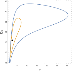
Figure 5: The model space of $\tau$ and ${\cal D}_{0}$ (taken to be April 14) from the data set for April 15–19. Retrospective changes to the data may be possible. The best fit (modal values) is denoted by the black dot. The inner curve encloses the 95% CrI, and the outer one the 99% CrI.

III.4 After April 14— incomplete data

We have noted earlier that retrospective changes are expected often to the most recent fatality data. This is why the analysis of the data for April 15–19 is made separately. Taking day zero to be April 14, we find

$$\tau=2.6{\rm\ days},\qquad{\rm and}\qquad{\cal D}_{0}=1.59.$$ (8)

The joint 95% CrI of the parameters is shown in Figure 5. The doubling time is half of that in eq. (7), implying an uncontrolled growth rate for the epidemic. There is less than a 11% chance that this doubling rate is compatible with that in eq. (7). Even more disturbing is that ${\cal D}_{0}$ is very low, with a negligible chance (less than one part in $10^{-30}$) that it is compatible with the lower bound on the 95% CrI of fatalities allowed by eq. (7) on April 14. It is clear from this that the data is either not yet complete, or that we are confronted with a huge statistical deviation away from the previous part of the same time series.

IV Conclusions

IV.1 The doubling time

The time series of data on fatalities in Mumbai was used to extract several characteristics of the epidemic in Mumbai. The most robust parameter that comes out of this is the doubling time, $\tau=5.3$ days (median, with $[4.6,6.9]$ 95% CrI). It is surprising that this rate of growth for COVID-19 is seen during the lock down. It is comparable to the doubling times reported in the early days of the epidemic in Wuhan, before a quarantine was imposed there sfr .

We also infer a parameter ${\cal D}_{0}$ which is the number of estimated fatalities on day zero of the analysis, which we take to me March 30. We find ${\cal D}_{0}=1.8$ (95% CrI, 1.4–2.4). This is in good agreement with the reported number of 2 on May 30. We note that this agreement indicates that the stochasticity in daily numbers is weak. One supporting evidence is that the cumulative count of fatalities has grown very smoothly over this period with the same doubling time as found here. This is a direct check that the assumption of exponential growth remains valid.

IV.2 Estimation of $R_{0}$

The doubling time can be matched to the basic reproduction rate, $R_{0}$, in different epidemiological models. Here we match it to a simple SEIR model. This has been used widely to model the COVID-19 epidemic, since the disease is non-infective in the incubation state. In the early stages of an epidemic, when the fraction of susceptibles in the population is close to unity, one may write

$$R_{0}=1+\log 2\,\left(\frac{t_{2}}{\tau}\right),$$ (9)

where the distribution of $t_{2}$ used is given after eq. (4). Using the value of $\tau$ quoted in eq. (7), we find $R_{0}=3.4$ (median) and $[2.4,4.8]$ 95% CrI. This is consistent with estimates from a range of countries, but closer to the upper edge of the global spread in values. Note that the only inputs here are the doubling time $\tau$ and the case resolution time $t_{2}$. There are public health implications which we discuss later.

IV.3 Counts of positive tested population

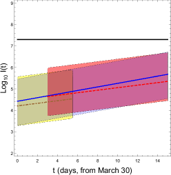
Figure 6: A Bayesian estimate of the number of infections in Mumbai. The region in yellow shows the $95\%{\rm\ CrI\/}$ of the estimated number of infections inferred from the number of fatalities observed until April 4. The brown dash-dotted line shows the median of the distribution. The area in pink is the 95% CrI based on data on fatalities from April 6 onwards, and its median is shown by the red dashed line. Note the reasonable agreement in the dates of overlap. The band in blue is the 95% CrI for the combined analysis after correcting for improved surveillance soon after April 2. The blue line is the median from this distribution. The horizontal black line is the population of Mumbai.

The process of extracting $I_{0}$ is indirect, since it depends on three different epidemiological parameters which require studies with patient databases more extensive than available in Mumbai now. We have taken them from ifr .The 95% CrI shown in Figure 6 should be understood as containing these uncertainties according to eq. (4).

MCGM’s daily counts of test positives, $T_{+}(t)$, for Mumbai over the period of March 31 to April 14 were analyzed with exactly the same methods which were applied to $D(t)$. It was found that the doubling time, $\tau$, was 5.7 days (modal value). The modal number of test positives on March 30 was inferred to be ${\cal T}_{0}=33$. Given the estimated $I_{0}$ on that day eq. (7), $\Pi=T_{+}(t)/I(t)$ can easily be estimated. It was found that on day zero $\Pi=0.13$% (median). Since the doubling time of the numerator and denominator are the same, this ratio has remained constant through the epidemic.

Without a massive increase in the number of tests, there is no direct way to verify the estimates of infections presented here. Several alternatives have been proposed, ranging from testing viral load in sewage paris to conducting sample surveys using different testing methods. An example of the latter is a recent serological sample study seroprev in California, USA. This study reported $\Pi$ to be 1.1–2%. When the test rate, i.e., the number of tests administered per million of population is small, $\Pi$ is proportional to the test rate. On April 18, India’s cumulative test rates were $2.69\times 10^{-4}$, USA had test rates of $1.1159\times 10^{-2}$ ourworld . If the Indian test rate is scaled up to the same value as the US, then, with the estimates of $\Pi$ presented in the previous paragraph would have to be multiplied by a factor of 42. This scaled value of $\Pi$ for Mumbai is compatible with that reported for California in seroprev .

IV.4 Dating the beginning of the epidemic

Given $\tau=5.3$ days, we can extrapolate from $I_{0}$ backwards to find when there was only a single case in Mumbai. This estimates the first seeding of COVID-19 in the city. We find that the median date for the initial seeding was around January 15, 2020. However, there is a 95% chance that the initial seeding occurred as early as December 20, 2019 or as late as February 1, 2020. Although the volume of traffic from China to Mumbai is not large, it is steady, and early seeding is not inconceivable, especially if the virus was spreading inside China already in mid-November. The first fatalities due to this cryptic spread of COVID-19 would not have happened before mid-February (median estimate). It is certainly possible to check municipal records of deaths in February to see whether any excesses over the same month in previous years are visible. If there is a statistically significant signal, it would support the idea of early cryptic seeding of COVID-19 in Mumbai.

IV.5 Public health implications

It is interesting that the value of $R_{0}$ deduced from the growth rate during a lock down is among the higher end of values seen in other countries. The purpose of this drastic measure was to reduce the value of $R_{0}$. This could be an indication that the epidemic growth is being driven by high density areas where physical distancing is impossible. It would be important to understand the structure in finer detail, ward-wise or at even finer scales, if possible. If there is indeed such geographical structure to the epidemic within Mumbai, then it is possible that post-lock down there could be a “second wave” surge of cases in areas where housing density is lower. Active steps must be taken to prevent this. The Maharashtra Government order of April 18, removing all relaxations of lock down in the Mumbai and Pune regions gomo may be seen in this context.

It should be noted that a significant fraction of the infected could be asymptomatic diapr ; evacu ; cdc . In this connection note that the symptom fatality ratio, ${\rm SFR\/}$, defined as the probability of dying after the onset of symptoms is reported to be 1.4% (median) $[0.9\%,2.1\%]$ 95% CrI sfr . Comparing this to the ${\rm IFR\/}$ of 0.657% gives an estimate of the probability of being asymptomatic: $P_{A}=1-{\rm IFR\/}/{\rm SFR\/}$. This is about 50%, and in the range quoted in literature. So it is possible that half the cases are not of significance for public health measures cdc ; who . Symptomatic cases are of significance. For these contact tracing, where possible, and quarantine, otherwise, remain the best tools available now for controlling spread by bringing down the growth rate.

However, the asymptomatic fraction is of importance for a long term solution to the COVID-19 epidemic. Barring a sudden discovery and large-scale deployment of a cure or vaccine, the epidemic can be only be stopped when the number of infected reaches a level where herd immunity begins to operate. Asymptomatic infections have to be counted in this. From this point of view one should see the upper ends of the bands in Figure 6 as the most optimistic scenarios for reaching this desirable end state to the epidemic.

Note that if the growth rate is not controlled quickly, the situation could become much worse. With the estimate of $R_{0}$ made here, it should be expected that herd immunity sets in when 71% (median and $[58\%,79\%]$ 95% CrI) of the population has been infected. Given ${\rm IFR\/}=0.657$%, this could imply around 100,000 fatalities in Greater Mumbai until herd immunity is reached. Note that conclusions like this may be model dependent. This extremely simple model is quoted here only for orientation.

Another way to look at these predictions is the following. The fatality rates till now have not been severe. However, at the current rate of doubling, it would take about 15 days for them to climb about 10-fold. This increase would give about 100 fatalities a day, and could climb above that. This is in the range of the peak number of daily COVID-19 fatalities in New York City nychealth .

If the fatality rate increases to such levels, the number of cases requiring critical care increases even more. Also critical care lasts longer for cases which recover. In the hypothetical cases discussed here, COVID-19 wards in the city would have to deal with several hundred admissions a day with care periods for each case ranging up to two months. Again, using the estimates given above, these rates would be reached in two to four weeks if the rate of growth of the epidemic does not come down.

V Acknowledgements

I would like to thank Basudeb Dasgupta, Sandeep Krishna, S. Krishnaswamy, Rajdeep Sensarma, and R. Shankar for careful readings of the manuscripts and useful suggestions, and the ISRC (Indian Scientists’ Response to COVID-19) mailing list for generating questions.

References

- (1) New York City Health Services website [https://www1.nyc.gov/site/doh/covid/covid-19-data.page]
- (2) Maurice Tamman, At-home COVID-19 deaths may be significantly undercounted in New York City, Reuters, April 8, 2020. [https://in.reuters.com/article/health-coronavirus-fdny/at-home-covid-19-deaths-may-be-significantly-undercounted-in-new-york-city-idINKBN21Q0E4]
- (3) A. Galeotti, P. Surico, S. Hohmann, How many people really die from COVID-19? Lessons from Italy, Forbes, April 6, 2020. [https://www.forbes.com/sites/lbsbusinessstrategyreview/2020/04/06/how-many-people-have-really-died-from-covid-19/]
- (4) R. Verity, et al., Estimates of the severity of Coronavirus disease 2019: a model based analysis, Lancet Infectious Diseases, (2020) [https://doi.org/10.1016/S1473-3099(20)30243-7]
- (5) E. Bendavid et al., COVID-19 Antibody Seroprevalence in Santa Clara County, California, medRxiv preprint April 11, 2020. [https://doi.org/10.1101/2020.04.14.20062463].
- (6) P. D. Yadav, V. A. Potdar, M. L. Choudhary, et al., Full-genome sequences of the first two SARS-CoV-2 viruses from India, Indian J Med Res [Epub ahead of print] [cited 2020 Apr 22]. [http://www.ijmr.org.in/preprintarticle.asp?id=281471]
- (7) P. Harsha, data set available at https://docs.google.com/spreadsheets/d/1-OYukZzMlRcRKfMqh-pAle0JYAjLjUy08N9V6S51sq0/
- (8) S. Gupta and A. Lahiri, Ground state , Eur. Phys. Lett., 128, 1, 11003 (2019); eprint arxiv:1910.11384. [doi:10.1209/0295-5075/128/11003]
- (9) S. Gupta and R. Shankar, Estimating the number of COVID-19 infections in Indian hot-spots using fatality data, eprint arxiv:2004.04025 [https://arxiv.org/pdf/2004.04025]
- (10) T. W. Russell, J. Hellewell, K. van Zandvoort, et al., Estimating the infection and case fatality ratio for coronavirus disease (COVID-19) using age-adjusted data from the outbreak on the Diamond Princess cruise ship, February 2020 Euro Surveill, 2020 Mar 25(12) [doi: 10.2807/1560-7917.ES.2020.25.12.2000256]
- (11) J. Oke and C. Heneghan, Global Covid-19 Case Fatality Rates, [https:/https://www.cebm.net/covid-19/global-covid-19-case-fatality-rates//www.cebm.net/covid-19/global-covid-19-case-fatality-rates/]
- (12) S. Goli and K. S. James, How much of SARS-CoV-2 Infections is India detecting? A model-based estimation, medRxiv preprint, April 15, 2020. [doi: https://doi.org/10.1101/2020.04.09.20059014]
- (13) S. A. Lauer, K. H. Grantz, Q. Bi, et al., Ann. Int. Med, 2020 [doi:10.7326/M20-0504]
- (14) Q. Li, X. Guan, P. Wu, et al., Early Transmission Dynamics in Wuhan, China, of Novel Coronavirus–Infected Pneumonia, N Eng J M ed, 2020; 382:1199-1207 [DOI: 10.1056/NEJMoa2001316]
- (15) T. Barnagarwala, State health officials criticise BMC as cases rise in Mumbai, Indian Express (Mumbai edition), April 2 (2020) 4. [https://epaper.indianexpress.com/2619796/Mumbai/April-03-2020]
- (16) J. T. Wu, K. Leung, M. Bushman, et al., Estimating clinical severity of COVID-19 from the transmission dynamics in Wuhan, China, Nature Medicine 26, 506–510 (2020) [https://doi.org/10.1038/s41591-020-0822-7]
- (17) S. Wurtzer, V. Marechal, J.-M. Mouchei, L. Moulin, Time course quantitative detection of SARS-CoV-2 in Parisian wastewaters correlates with COVID-19 confirmed cases, medRxiv preprint April 17, (2020) [doi https://doi.org/10.1101/2020.04.12.20062679]
- (18) Our World in Data, [https://ourworldindata.org/grapher/covid-19-tests-cases-scatter-with-comparisons]
- (19) Government of Maharashtra, Order no. DMU/2020/CR.92/DisM-1, April 18 (2020), Amendment to the Consolidated Revised Guidelines on the measures to be taken for containment of COVID-19 in the State.
- (20) K. Mizumoto, K. Kagaya, A. Zarebski and G. Chowell, Estimating the asymptomatic proportion of coronavirus disease 2019 (COVID-19) cases on board the Diamond Princess cruise ship, Yokohama, Japan, 2020, Euro Surveill. 2020 Mar 12; 25(10): 2000180. [doi: 10.2807/1560-7917.ES.2020.25.10.2000180]
- (21) H. Nishiura, T. Kobayashi, A. Suzuki, et al., Estimation of the asymptomatic ratio of novel coronavirus infections (COVID-19), Int J Infect Dis Published Online First: 13 March 2020. [doi:10.1016/j.ijid.2020.03.020]
- (22) US Centers for Disease Control, Interim Clinical Guidance for Management of Patients with Confirmed Coronavirus Disease (COVID-19), [https://www.cdc.gov/coronavirus/2019-ncov/hcp/clinical-guidance-management-patients.html]
- (23) WHO Coronavirus Disease 2019 (COVID-19) Situation Report-73, April 2, 2020. [https://Fwww.who.int/docs/default-source/coronaviruse/situation-reports/20200402-sitrep-73-covid-19.pdf]