Direct Evidence for Universal Statistics of Stationary Kardar-Parisi-Zhang Interfaces

Abstract

The nonequilibrium steady state of the one-dimensional (1D) Kardar-Parisi-Zhang (KPZ) universality class is studied in-depth by exact solutions, yet no direct experimental evidence of its characteristic statistical properties has been reported so far. This is arguably because, for an infinitely large system, infinitely long time is needed to reach such a stationary state and also to converge to the predicted universal behavior. Here we circumvent this problem in the experimental system of growing liquid-crystal turbulence, by generating an initial condition that possesses a long-range property expected for the KPZ stationary state. The resulting interface fluctuations clearly show characteristic properties of the 1D stationary KPZ interfaces, including the convergence to the Baik-Rains distribution. We also identify finite-time corrections to the KPZ scaling laws, which turn out to play a major role in the direct test of the stationary KPZ interfaces. This paves the way to explore unsolved properties of the stationary KPZ interfaces experimentally, making possible connections to nonlinear fluctuating hydrodynamics and quantum spin chains as recent studies unveiled relation to the stationary KPZ.

Introduction.

The Kardar-Parisi-Zhang (KPZ) universality class describes dynamic scaling laws of a variety of phenomena, ranging from growing interfaces to directed polymers and stirred fluids Kardar et al. (1986); Barabási and Stanley (1995), as well as fluctuating hydrodynamics Spohn (2016) and, most recently, quantum integrable spin chains Ljubotina et al. (2019); *Gopalakrishnan.Vasseur-PRL2019; *Das.etal-PRE2019, to name but a few. The KPZ class is now central in the studies of nonequilibrium scaling laws, mostly because some models in the one-dimensional (1D) KPZ class turned out to be integrable and exactly solvable (for reviews, see, e.g., Takeuchi (2018); Spohn (2017); *HalpinHealy.Takeuchi-JSP2015; *Corwin-RMTA2012). This has unveiled a wealth of nontrivial fluctuation properties in such nonequilibrium and nonlinear many-body problems.

The KPZ class is often characterized by the KPZ equation, a paradigmatic model for interfaces growing in fluctuating environments Kardar et al. (1986); Barabási and Stanley (1995); Takeuchi (2018). It reads, in the case of 1D interfaces in a plane:

$$\frac{\partial{}}{\partial{t}}h(x,t)=\nu\frac{\partial^{2}h}{\partial{x}^{2}}+\frac{\lambda}{2}\left(\frac{\partial{h}}{\partial{x}}\right)^{2}+\eta(x,t).$$ (1)

Here $h(x,t)$ denotes the position of the interface in the direction normal to a reference line (e.g., substrate), often called the local height, at lateral position $x$ and time $t$. $\eta(x,t)$ is white Gaussian noise with $\langle{\eta(x,t)}\rangle=0$ and $\langle{\eta(x,t)\eta(x^{\prime},t^{\prime})}\rangle=D\delta(x-x^{\prime})\delta(t-t^{\prime})$, where $\langle{\cdots}\rangle$ denotes the ensemble average. Such random growth develops nontrivial fluctuations of $h(x,t)$, characterized by a set of universal power laws. For example, the fluctuation amplitude of $h(x,t)$ grows as $t^{\beta}$, with $\beta=1/3$ for 1D. This implies

$$h(x,t)\simeq v_{\infty}t+(\Gamma t)^{1/3}\chi+\mathcal{O}(t^{0})$$ (2)

with constant parameters $v_{\infty},\Gamma$ and a rescaled random variable $\chi$. $\chi$ is correlated in space and time but characterized by a distribution that remains well defined in the limit $t\to\infty$. Another important quantity is the height-difference correlation function, defined by $C_{h}(\ell,t)\equiv\langle{[h(x+\ell,t)-h(x,t)]^{2}}\rangle$. While $C_{h}(\ell,t)\sim{}t^{2\beta}$ for $\ell$ much larger than the correlation length $\xi(t)\sim{}t^{1/z}$, for $\ell\ll\xi(t)$, $C_{h}(\ell,t)\sim{}\ell^{\,2\alpha}$ with $\alpha=z\beta$ Barabási and Stanley (1995); Takeuchi (2018). For 1D, the scaling exponents are $\alpha=1/2,\beta=1/3,z=3/2$ and shared among members of the KPZ universality class Kardar et al. (1986); Barabási and Stanley (1995); Takeuchi (2018); Corwin (2012). Moreover, for the 1D KPZ equation (1), the (statistically) stationary state of this particular model, $h_{\text{stat}}^{\text{KPZeq}}(x)$, is known to be equivalent to the 1D Brownian motion Kardar et al. (1986); Barabási and Stanley (1995); Takeuchi (2018); Corwin (2012):

$$h_{\text{stat}}^{\text{KPZeq}}(x)=\sqrt{A}B(x).$$ (3)

Here, $A\equiv{}D/2\nu$ and $B(x)$ is the standard Brownian motion with time $x$, so that $\langle{B(x)}\rangle=0$ and $\langle{[B(x+\ell)-B(x)]^{2}}\rangle=\ell$. The height-difference correlation function for $h_{\text{stat}}^{\text{KPZeq}}(x)$ is then simply the mean-squared displacement, $C_{h_{\text{stat}}^{\text{KPZeq}}}(\ell)\simeq{}A\ell$, with $A$ corresponding to the diffusion coefficient. Note that, even if we set $h(x,0)=h_{\text{stat}}^{\text{KPZeq}}(x)$, $h(x,t)$ still fluctuates and grows, i.e., $\langle{h(x,t)}\rangle=v_{\infty}t$ with a constant $v_{\infty}$. Nevertheless, the shifted height $h(x,t)-v_{\infty}t$ can be always described by Eq. (3) with another instance of $B(x)$ (which is actually correlated with the one used for the initial condition). For lack of a better term, here we call it the (statistically) stationary state of the KPZ equation.

Then the exact solutions of the 1D KPZ equation Sasamoto and Spohn (2010); Amir et al. (2011); Calabrese et al. (2010); Dotsenko (2010); Calabrese and Le Doussal (2011); Imamura and Sasamoto (2012); Borodin et al. (2015), as well as earlier results for discrete models (e.g., Johansson (2000); Prähofer and Spohn (2000)), unveiled detailed fluctuation properties of $h(x,t)$, in particular the distribution function of $\chi$ Takeuchi (2018); Corwin (2012). Further, those properties turned out to depend on the global geometry of interfaces or on the initial condition $h(x,0)$, being classified into a few universality subclasses within the single KPZ class. Among them, most important and established are the subclasses for circular, flat, and stationary interfaces, characterized by the following asymptotic distributions Takeuchi (2018): the GUE Tracy-Widom Tracy and Widom (1994), GOE Tracy-Widom Tracy and Widom (1996), and Baik-Rains distributions Baik and Rains (2000), respectively (GUE and GOE stand for the Gaussian unitary and orthogonal ensembles, respectively). More precisely, with the random numbers drawn from those distributions, denoted by $\chi_{2},\chi_{1},\chi_{0}$ , respectively, we have $\chi\stackrel{{\scriptstyle d}}{{\to}}\chi_{2},\chi_{1},\chi_{0}$ for the three respective subclasses , where $\stackrel{{\scriptstyle d}}{{\to}}$ indicates the convergence in the distribution. For the KPZ equation, the typical initial conditions that correspond to the three subclasses are $h(x,0)=-|x|/\delta~{}(\delta\to 0^{+})$ (circular), $h(x,0)=0$ (flat), and $h(x,0)=h_{\text{stat}}^{\text{KPZeq}}(x)=\sqrt{A}B(x)$ (stationary). Experimentally, the circular and flat subclasses were clearly observed in the growth of liquid-crystal turbulence Takeuchi and Sano (2010); *Takeuchi.etal-SR2011; Takeuchi and Sano (2012); Takeuchi (2018), but only indirect and partial support has been reported so far for the stationary subclass Takeuchi (2013, 2017) (see also ). This is presumably because, firstly, for an infinitely large system, it takes infinitely long time for a system to reach the stationary state (as $\xi(t)\sim{}t^{2/3}$ needs to reach infinity). Then one should take an interface profile in the stationary state, regard it as an “initial condition”, and wait sufficiently long time for the height fluctuations to converge to the Baik-Rains distribution (see Ref. Takeuchi (2013) for more quantitative arguments). For a finite system of size $L$, reaching the stationary state takes a finite time $\sim{}L^{3/2}$, but the approach to the Baik-Rains distribution is now visible only within a finite time period Prolhac (2016); Baik and Liu (2017), being eventually replaced by a final state unrelated to the choice of the initial condition.

Here we overcome this difficulty in the liquid-crystal experimental system, by generating an interface that resembles the expected stationary state. Using a holographic technique developed previously Fukai and Takeuchi (2017); *Fukai.Takeuchi-PRL2020, we generated Brownian initial conditions (3) for the growing turbulence and directly measured fluctuation properties of the height $h(x,t)$ under this type of initial conditions [Fig. 1(b)]. This allowed us to carry out quantitative tests of a wealth of exact results for integrable models in the stationary state. And indeed, we obtained direct evidence for the Baik-Rains distribution and the related correlation function. This opens an experimental pathway to explore universal yet hitherto unsolved statistical properties of the KPZ stationary state.

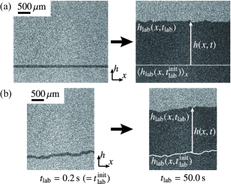
Figure 1: Typical snapshots of a flat (a) and a Brownian (b) interface, separating the metastable DSM1 (gray) and growing DSM2 regions (black). $h_{\text{lab}}(x,t_{\text{lab}})$ denotes the position of the upper interface in the laboratory frame, at time $t_{\text{lab}}$ from the laser emission. $t$ and $h(x,t)$ are defined as follows: $t\equiv{}t_{\text{lab}}$ and $h(x,t)\equiv{}h_{\text{lab}}(x,t_{\text{lab}})-\langle{h(x,t_{\text{lab}}^{\text{init}})}\rangle_{x}$ for the flat case (a), $t\equiv{}t_{\text{lab}}-t_{\text{lab}}^{\text{init}}$ and $h(x,t)\equiv{}h(x,t_{\text{lab}})-h(x,t_{\text{lab}}^{\text{init}})$ for the Brownian case (b). See also Movies S1 and S2 SM .

Methods.

The experimental system was a minor modification of that used in Ref. Fukai and Takeuchi (2017); *Fukai.Takeuchi-PRL2020 (see Sec. I of Supplementary Text and Fig. S1 SM for details). We used a standard material for the electroconvection of nematic liquid crystal de Gennes and Prost (1995), specifically, $N$-(4-methoxybenzylidene)-4-butylaniline doped with tetra-$n$-butylammonium bromide. The liquid crystal sample was placed between two parallel glass plates with transparent electrodes, separated by spacers of thickness $12~{}\mathrm{\mu{}m}$. The electrodes were surface-treated to realize homeotropic alignment. The temperature was maintained at $25~{}\mathrm{{}^{\circ}{}C}$ during the experiments, with typical fluctuations of $0.01~{}\mathrm{{}^{\circ}{}C}$.

The electroconvection was induced by applying an ac voltage to the system. In this work we fixed the frequency at $250~{}\mathrm{Hz}$, well below the cut-off frequency near $1.8~{}\mathrm{kHz}$, and the voltage was set to be $23~{}\mathrm{V}$. At this voltage, the system is initially in a turbulent state called the dynamic scattering mode 1 (DSM1), which is actually metastable, so that the stable turbulent state DSM2 eventually nucleates and expands, forming a growing cluster bordered by a fluctuating interface. One can also trigger DSM2 nucleation by shooting an ultraviolet (UV) laser pulse Takeuchi (2018). This not only allows us to carry out controlled experiments but also to design the initial shape of the interface, by changing the intensity profile of the laser beam. Growing interfaces were observed by recording light transmitted through the sample, using a light-emitting diode as the light source and a charge-coupled device camera.

Flat interface experiments.

In order to realize Brownian initial conditions (3) that may correspond to the stationary state, we first need to evaluate the parameter $A$. To this end we first carried out a set of experiments for flat interfaces. Using a cylindrical lens to expand the laser beam, we generated an initially straight interface for each experiment and tracked growth of the upper interface [Fig. 1(a)]. The $h$-axis is set along the mean growth direction. The $x$-axis is normal to $h$, along the initial straight line. Then the coordinates of the upper interface in the laboratory frame were extracted and denoted by $h_{\text{lab}}(x,t_{\text{lab}})$, where $t_{\text{lab}}$ is the time elapsed since the laser emission. Since the height of interest is the increment from the initial interface, we approximated it by the spatially averaged height at the first analyzable time, denoted by $\langle{h(x,t_{\text{lab}}^{\text{init}})}\rangle_{x}$, with $t_{\text{lab}}^{\text{init}}=0.2~{}\mathrm{s}$. Then we defined $h(x,t)\equiv{}h_{\text{lab}}(x,t_{\text{lab}})-\langle{h(x,t_{\text{lab}}^{\text{init}})}\rangle_{x}$ with $t\equiv{}t_{\text{lab}}$ and studied its fluctuations over 1267 independent realizations. In the following, the ensemble average $\langle{\cdots}\rangle$ was evaluated by averaging over all realizations and spatial points $x$.

The parameter $A$ can be determined by the relation $A=\sqrt{2\Gamma/v_{\infty}}$, known to hold in isotropic systems Takeuchi and Sano (2012); Takeuchi (2018). For $v_{\infty}$, we followed the standard procedure Krug et al. (1992); Takeuchi (2018) and plotted $\frac{\mathrm{d}\langle{h}\rangle}{\mathrm{d}t}$ against $t^{-2/3}$ [Fig. 2(a) main panel]. From Eq. (2), we have

$$\frac{\mathrm{d}\langle{h}\rangle}{\mathrm{d}t}\simeq v_{\infty}+\frac{\Gamma^{1/3}\langle{\chi}\rangle}{3}t^{-2/3}.$$ (4)

Therefore, reading the $y$-intercept of linear regression, we obtained $v_{\infty}=36.86(4)~{}\mathrm{\mu{}m/s}$, where the numbers in the parentheses indicate the uncertainty. For $\Gamma$, since the flat interfaces in this liquid-crystal system were already shown to exhibit the GOE Tracy-Widom distribution Takeuchi et al. (2011); Takeuchi and Sano (2012); Takeuchi (2018), we have $\langle{h^{n}}\rangle_{\mathrm{c}}\simeq(\Gamma{}t)^{n/3}\langle{\chi_{1}^{n}}\rangle_{\mathrm{c}}(n\geq 2)$, where $\langle{X^{n}}\rangle_{\mathrm{c}}$ denotes the $n$th-order cumulant of a variable $X$. Above all, the variance can be most precisely determined, and is known to grow, with the leading finite-time correction, as $\langle{h^{2}}\rangle_{\mathrm{c}}\simeq(\Gamma{}t)^{2/3}\langle{\chi_{1}^{2}}\rangle_{\mathrm{c}}+\mathcal{O}(t^{0})$ Takeuchi and Sano (2012); Takeuchi (2018); Ferrari and Frings (2011). Therefore, by plotting $\langle{h^{2}}\rangle_{\mathrm{c}}t^{-2/3}$ against $t^{-2/3}$ [Fig. 2(a) inset] and reading the $y$-intercept of linear regression, we obtained $\Gamma=1415(4)~{}\mathrm{\mu{}m^{3}/s}$ . Consistency was checked by plotting the histogram of the height, rescaled with those parameters as follows

$$q(x,t)\equiv\frac{h(x,t)-v_{\infty}t}{(\Gamma t)^{1/3}}\simeq\chi.$$ (5)

Clear agreement with the GOE Tracy-Widom distribution was confirmed [Fig. 2(b)]. Using those estimates, we finally obtained $A=\sqrt{2\Gamma/v_{\infty}}=8.762(13)~{}\mathrm{\mu{}m}$.

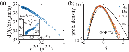
Figure 2: Parameter estimation for the flat interfaces. (a) $\frac{\mathrm{d}\langle{h}\rangle}{\mathrm{d}t}$ against $t^{-2/3}$ (main panel) and $\langle{h^{2}}\rangle_{\mathrm{c}}t^{-2/3}$ against $t^{-2/3}$ (inset). The dashed lines show the results of linear regression. (b) Histograms of the rescaled height $q(x,t)$ at different $t$ (legend). Agreement with the GOE Tracy-Widom (TW) distribution is confirmed. BR stands for the Baik-Rains distribution.

Brownian interface experiments.

Based on the value of $A$ evaluated by the flat interface experiments, we generated Brownian initial conditions (3) with $A=9~{}\mathrm{\mu{}m}$ and studied growing DSM2 interfaces [Fig. 1(b)]. Each initial condition was prepared by projecting a hologram of a computer-generated Brownian trajectory, with resolution of $36.5~{}\mathrm{\mu{}m}$ at the liquid-crystal cell, by using a spatial light modulator SM . The height profile in the laboratory frame $h_{\text{lab}}(x,t_{\text{lab}})$ was determined as for the flat experiments, but here the height of interest is the increment from the height profile at the first analyzable time, $h(x,t)\equiv{}h_{\text{lab}}(x,t_{\text{lab}})-h_{\text{lab}}(x,t_{\text{lab}}^{\text{init}})$, with $t\equiv{}t_{\text{lab}}-t_{\text{lab}}^{\text{init}}$ and $t_{\text{lab}}^{\text{init}}=0.2~{}\mathrm{s}$ [Fig. 1(b)]. We used a region of width $2730~{}\mathrm{\mu{}m}$ near the center of the camera view and analyzed 1021 interfaces. Finite-size effect is expected to be prevented, because the Brownian trajectories were much longer ($4670~{}\mathrm{\mu{}m}$ in $x$) than the width of the analyzed region.

First we test whether the interfaces generated thereby are stationary or not. To this end, we measure the height-difference correlation function for $h_{\text{lab}}(x,t_{\text{lab}})$, $C_{h_{\text{lab}}}(\ell,t_{\text{lab}})$, and find that it does depend on $t_{\text{lab}}$ [Fig. 3(a)], indicating that the interfaces are not stationary. More precisely, we observe that $C_{h_{\text{lab}}}(\ell,t_{\text{lab}})/\ell$ at small $\ell$ initially takes values lower than the desired one, $A=9~{}\mathrm{\mu{}m}$, presumably because of the finite resolution of the holograms, then increases up to $\approx{}11~{}\mathrm{\mu{}m}$. The fact that $C_{h_{\text{lab}}}(\ell,t_{\text{lab}})/\ell$ becomes higher than $A$ at small $\ell$ was also observed in our flat data [Fig. 3(a) inset] as well as in our past experiments Takeuchi and Sano (2010); Takeuchi (2018). However, more important is the behavior at large $\ell$, which turns out to be stable and takes a value close to $A=9~{}\mathrm{\mu{}m}$. Therefore, in the following we test whether our interfaces, though not stationary, can nevertheless exhibit universal properties of the stationary KPZ subclass, such as the Baik-Rains distribution.

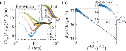
Figure 3: Evaluation of the Brownian interfaces. (a) $C_{h_{\text{lab}}}(\ell,t_{\text{lab}})/\ell$ against $\ell$ for different $t_{\text{lab}}$ (indicated in the legends) for the Brownian (main panel) and flat (inset) interfaces. The black stars indicate the results of direct evaluation of the computer-generated images used for the holograms. (b) $\frac{\mathrm{d}\langle{h}\rangle}{\mathrm{d}t}$ against $t^{-4/3}$ (main panel) and $t^{-2/3}$ (inset) for the Brownian interfaces. The dashed line in the main panel shows the result of linear regression.

To determine the scaling coefficients, we plot $\frac{\mathrm{d}\langle{h}\rangle}{\mathrm{d}t}$ against $t^{-2/3}$ in the inset of Fig. 3(b). Time dependence of $\frac{\mathrm{d}\langle{h}\rangle}{\mathrm{d}t}$ confirms non-stationarity of the interfaces again. Interestingly, as opposed to the result for the flat interfaces [Fig. 2(a)], here we do not find linear relationship to $t^{-2/3}$ [Fig. 3(b) inset], but to $t^{-4/3}$ (main panel). From Eq. (4), this suggests $\langle{\chi}\rangle=0$, consistent with the vanishing mean of the Baik-Rains distribution $\langle{\chi_{0}}\rangle=0$. If so, the subleading term of Eq. (4) is indeed expected to be $\mathcal{O}(t^{-4/3})$, coming from a $t^{-1/3}$ term expected to exist in Eq. (2). Then, by linear regression, we obtained $v_{\infty}=37.126(15)~{}\mathrm{\mu{}m/s}$. It is reasonably close to the value from the flat experiments, in view of the typical magnitude of parameter shifts in this experimental system Takeuchi and Sano (2012). For $\Gamma$, we took the value from the flat experiments, so that we do not make any assumption on the statistical properties for the Brownian case.

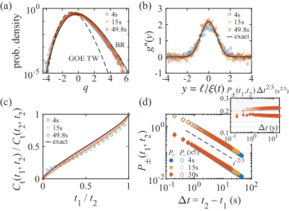
Figure 4: Main results of the Brownian interface experiments. (a) Histograms of the rescaled height $q(x,t)$ at different $t$ (legend). The data are found to converge to the Baik-Rains (BR) distribution, as shown quantitatively in Sec. II of Supplementary Text and Fig. S2 SM . GOE TW stands for the GOE Tracy-Widom distribution. (b) Two-point correlation function $g^{\prime\prime}(y)$. The experimental data are evaluated by $\frac{\xi(t)^{2}}{(\Gamma{}t)^{2/3}}2\langle{\frac{\partial{{h_{\text{lab}}}}}{\partial{x}}(\ell+x,t+{t_{\text{lab}}^{\text{init}}})\frac{\partial{{h_{\text{lab}}}}}{\partial{x}}(x,{t_{\text{lab}}^{\text{init}}})}\rangle$ with different $t$ (legend). The black curve indicates Prähofer and Spohn’s exact solution Prähofer and Spohn (2004); Pra . (c) Rescaled two-time function $C_{\mathrm{t}}(t_{1},t_{2})/C_{\mathrm{t}}(t_{2},t_{2})$ for different $t_{2}$ (legend). The data are found to converge to Ferrari and Spohn’s exact solution Ferrari and Spohn (2016) (black curve), as shown quantitatively in Sec. III of Supplementary Text and Fig. S3 SM . (d) Persistence probability $P_{\pm}(t_{1},t_{2})$ for different $t_{1}$ (legend). For visibility, $P_{-}(t_{1},t_{2})$ is shifted by factor $5$. The dashed line is a guide for eyes indicating the power law $t^{-2/3}$ for FBM_1/3. The inset shows $P_{\pm}(t_{1},t_{2})\Delta{}t^{2/3}$.

Using the values of $v_{\infty}$ and $\Gamma$ determined thereby, as well as $A=\sqrt{2\Gamma/v_{\infty}}$, we test various predictions for the stationary KPZ subclass, without any adjustable parameter. The results are summarized in Fig. 4. Figure 4(a) shows histograms of the rescaled height $q(x,t)$ [Eq. (5)] at different times $t$. The obtained distributions at finite times are already close to the predicted Baik-Rains distribution. Indeed, convergence in the $t\to\infty$ limit is confirmed quantitatively by analyzing finite-time corrections in the cumulants (Sec. II of Supplementary Text and Fig. S2 SM ). In Fig. 4(b), we test the prediction on the two-point correlation function $C_{2}(\ell,t)\equiv\langle{[{h_{\text{lab}}}(\ell+x,t+t_{0})-{h_{\text{lab}}}(x,t_{0})-v_{\infty}{}t]^{2}}\rangle$. It is often denoted by $g(y)$ in the rescaled units, with $y\equiv\ell/\xi(t)$, $\xi(t)\equiv(2/A)(\Gamma{}t)^{2/3}$, and $g(y)\equiv(\Gamma{}t)^{-2/3}C_{2}(\ell,t)$. Its second derivative, $g^{\prime\prime}(y)$, plays the pivotal role in the emergence of KPZ in fluctuating hydrodynamics Spohn (2016) and quantum integrable spin chains Ljubotina et al. (2019). This is tested with our experimental data and good agreement is found [Fig. 4(b)]. Figure 4(c) shows the results of the two-time correlation of $h(x,t)$, $C_{\mathrm{t}}(t_{1},t_{2})\equiv\langle{\delta{}h(x,t_{1})\delta{}h(x,t_{2})}\rangle$ with $\delta{}h(x,t)\equiv{}h(x,t)-\langle{h(x,t)}\rangle$. Our data agree with Ferrari and Spohn’s prediction Ferrari and Spohn (2016) that the two-time correlation coincides with that of the fractional Brownian motion with Hurst exponent $1/3$ (hereafter abbreviated to FBM_1/3), $C_{\mathrm{t}}(t_{1},t_{2})/C_{\mathrm{t}}(t_{2},t_{2})\to(1/2)[1+(t_{1}/t_{2})^{2/3}-(1-t_{1}/t_{2})^{2/3}]$ (black line) in the limit $t_{1},t_{2}\to\infty$ with fixed $t_{1}/t_{2}$ (see Sec. III of Supplementary Text and Fig. S3 SM for a quantitative test). Finally, Fig. 4(d) shows the persistence probability $P_{\pm}(t_{1},t_{2})$, i.e., the probability that $h(x,t)-h(x,t_{1})$ remains always positive ($P_{+}$) or negative ($P_{-}$) until time $t_{2}$, which is found to decay clearly as $P_{\pm}(t_{1},t_{2})\sim{}\Delta{}t^{-2/3}$ with $\Delta{}t\equiv{}t_{2}-t_{1}$. The persistence exponent is therefore $2/3$, supporting Krug et al.’s conjecture Krug et al. (1997); *Kallabis.Krug-EL1999; *Bray.etal-AP2013 that it also coincides with that of FBM_1/3. Those relations to FBM_1/3  are intriguing, because $h(x,t)$ is not Gaussian and therefore its time evolution is not FBM_1/3.

Concluding remarks.

In this work we aimed at unambiguous tests of universal statistics for the stationary state of the $(1+1)$-dimensional KPZ class. Instead of waiting for the interfaces to approach the stationary state, we generated such initial conditions that are expected to share the same long-range properties with the stationary state, specifically, the Brownian initial conditions (3) with the appropriate diffusion coefficient $A$ determined beforehand. The resulting interfaces turned out to be not stationary, but nevertheless our data clearly showed the defining properties of the stationary KPZ subclass, including the Baik-Rains distribution and the two-point correlation function $g^{\prime\prime}(y)$ [Fig. 4(a)(b)]. Our results also support intriguing relations to time correlation properties of the fractional Brownian motion [Fig. 4(c)(d)], which may deserve further investigations in other quantities. With this and past studies Takeuchi and Sano (2010); Takeuchi et al. (2011); Takeuchi and Sano (2012); Takeuchi (2018), all the three representative KPZ subclasses in one dimension Takeuchi (2018); Corwin (2012) were given experimental supports for the universality.

The KPZ class has been extensively studied already for decades, yet it continues finding novel connections to various areas of physics (recall recent developments in nonlinear fluctuating hydrodynamics Spohn (2016) and quantum spin chains Ljubotina et al. (2019)). We hope our experiments will also serve to probe quantities of interest for those systems, which may be not always solved exactly but still have a possibility to be measured precisely. Explorations of higher dimensions, for which numerics have played leading roles Halpin-Healy (2012); *HalpinHealy-PRE2013; *Oliveira.etal-PRE2013; Halpin-Healy and Takeuchi (2015), are also important directions left for future studies.

References

- Kardar et al. (1986) M. Kardar, G. Parisi, and Y.-C. Zhang, Phys. Rev. Lett. 56, 889 (1986).
- Barabási and Stanley (1995) A.-L. Barabási and H. E. Stanley, Fractal Concepts in Surface Growth (Cambridge Univ. Press, Cambridge, 1995).
- Spohn (2016) H. Spohn, in Thermal Transport in Low Dimensions, Lecture Notes in Physics, Vol. 921, edited by S. Lepri (Springer, Heidelberg, 2016) Chap. 3, pp. 107–158, arXiv:1505.05987 .
- Ljubotina et al. (2019) M. Ljubotina, M. Žnidarič, and T. Prosen, Phys. Rev. Lett. 122, 210602 (2019).
- Gopalakrishnan and Vasseur (2019) S. Gopalakrishnan and R. Vasseur, Phys. Rev. Lett. 122, 127202 (2019).
- Das et al. (2019) A. Das, M. Kulkarni, H. Spohn, and A. Dhar, Phys. Rev. E 100, 042116 (2019).
- Takeuchi (2018) K. A. Takeuchi, Physica A 504, 77 (2018).
- Spohn (2017) H. Spohn, in Stochastic Processes and Random Matrices, Lecture Notes of the Les Houches Summer School, Vol. 104, edited by G. Schehr, A. Altland, Y. V. Fyodorov, N. O’Connell, and L. F. Cugliandolo (Oxford Univ. Press, Oxford, 2017) Chap. 4, pp. 177–227, arXiv:1601.00499 .
- Halpin-Healy and Takeuchi (2015) T. Halpin-Healy and K. A. Takeuchi, J. Stat. Phys. 160, 794 (2015).
- Corwin (2012) I. Corwin, Random Matrices Theory Appl. 1, 1130001 (2012).
- Sasamoto and Spohn (2010) T. Sasamoto and H. Spohn, Phys. Rev. Lett. 104, 230602 (2010).
- Amir et al. (2011) G. Amir, I. Corwin, and J. Quastel, Commun. Pure Appl. Math. 64, 466 (2011).
- Calabrese et al. (2010) P. Calabrese, P. Le Doussal, and A. Rosso, Europhys. Lett. 90, 20002 (2010).
- Dotsenko (2010) V. Dotsenko, Europhys. Lett. 90, 20003 (2010).
- Calabrese and Le Doussal (2011) P. Calabrese and P. Le Doussal, Phys. Rev. Lett. 106, 250603 (2011).
- Imamura and Sasamoto (2012) T. Imamura and T. Sasamoto, Phys. Rev. Lett. 108, 190603 (2012).
- Borodin et al. (2015) A. Borodin, I. Corwin, P. Ferrari, and B. Vető, Math. Phys. Anal. Geom. 18, 20 (2015).
- Johansson (2000) K. Johansson, Commun. Math. Phys. 209, 437 (2000).
- Prähofer and Spohn (2000) M. Prähofer and H. Spohn, Phys. Rev. Lett. 84, 4882 (2000).
- Tracy and Widom (1994) C. A. Tracy and H. Widom, Commun. Math. Phys. 159, 151 (1994).
- Tracy and Widom (1996) C. A. Tracy and H. Widom, Commun. Math. Phys. 177, 727 (1996).
- Baik and Rains (2000) J. Baik and E. M. Rains, J. Stat. Phys. 100, 523 (2000).
- Note (1) With the standard GOE Tracy-Widom random variable (as defined in Ref. Tracy and Widom (1996)), is defined by Takeuchi (2018).
- Note (2) In the circular case, for , an additional shift proportional to is needed for the convergence to , to compensate the locally parabolic mean profile of the interfaces Takeuchi (2018); Spohn (2017). In the stationary case, the left-hand side of Eq. (2) should be more precisely , but by imposing one can still use Eq. (2) with to show Takeuchi (2018); Spohn (2017).
- Takeuchi and Sano (2010) K. A. Takeuchi and M. Sano, Phys. Rev. Lett. 104, 230601 (2010).
- Takeuchi et al. (2011) K. A. Takeuchi, M. Sano, T. Sasamoto, and H. Spohn, Sci. Rep. 1, 34 (2011).
- Takeuchi and Sano (2012) K. A. Takeuchi and M. Sano, J. Stat. Phys. 147, 853 (2012).
- Takeuchi (2013) K. A. Takeuchi, Phys. Rev. Lett. 110, 210604 (2013).
- Takeuchi (2017) K. A. Takeuchi, J. Phys. A 50, 264006 (2017).
- Note (3) There was a claim for an observation of the Baik-Rains distribution in an experiment of paper combustion Miettinen et al. (2005), but it seems to us that their precision is not sufficient to distinguish it from other possible distributions, as detailed in the commentary article available at http://publ.kaztake.org/miet-com.pdf. Note also that in the stationary state of a finite-size system, as studied in this experiment, an approach to the Baik-Rains distribution will appear in a finite time window, so that careful analysis of time dependence is crucial.
- Prolhac (2016) S. Prolhac, Phys. Rev. Lett. 116, 090601 (2016).
- Baik and Liu (2017) J. Baik and Z. Liu, Commun. Pure Appl. Math. 71, 747 (2017).
- Fukai and Takeuchi (2017) Y. T. Fukai and K. A. Takeuchi, Phys. Rev. Lett. 119, 030602 (2017).
- Fukai and Takeuchi (2020) Y. T. Fukai and K. A. Takeuchi, Phys. Rev. Lett. 124, 060601 (2020).
- (35) See Supplemental Material at [URL] for Supplementary Text (Sec. I-III), Figs. S1-S3, and Movies S1 and S2. Ref. De Nardis et al. (2017) is cited therein.
- de Gennes and Prost (1995) P. G. de Gennes and J. Prost, The Physics of Liquid Crystals, 2nd ed., International Series of Monographs on Physics, Vol. 83 (Oxford Univ. Press, New York, 1995).
- Krug et al. (1992) J. Krug, P. Meakin, and T. Halpin-Healy, Phys. Rev. A 45, 638 (1992).
- Ferrari and Frings (2011) P. L. Ferrari and R. Frings, J. Stat. Phys. 144, 1123 (2011).
- Note (4) Although can also be estimated from Eq. (4), reading the slope of Fig. 2(a) is much less precise than the estimation based on the variance.
- Note (5) To reduce the effect of parameter shift, we chose to start the Brownian interface experiments before completing the careful analysis of the flat experimental data. As a result, we used a rough estimate for the Brownian initial conditions. Slight difference in is expected to have only a minor impact on the fluctuation properties of Chhita et al. (2018).
- Prähofer and Spohn (2004) M. Prähofer and H. Spohn, J. Stat. Phys. 115, 255 (2004).
- (42) Theoretical curves available in the following URL were used: https://www-m5.ma.tum.de/KPZ.
- Ferrari and Spohn (2016) P. L. Ferrari and H. Spohn, SIGMA 12, 074 (2016).
- Krug et al. (1997) J. Krug, H. Kallabis, S. N. Majumdar, S. J. Cornell, A. J. Bray, and C. Sire, Phys. Rev. E 56, 2702 (1997).
- Kallabis and Krug (1999) H. Kallabis and J. Krug, Europhys. Lett. 45, 20 (1999).
- Bray et al. (2013) A. J. Bray, S. N. Majumdar, and G. Schehr, Adv. Phys. 62, 225 (2013).
- Halpin-Healy (2012) T. Halpin-Healy, Phys. Rev. Lett. 109, 170602 (2012).
- Halpin-Healy (2013) T. Halpin-Healy, Phys. Rev. E 88, 042118 (2013).
- Oliveira et al. (2013) T. J. Oliveira, S. G. Alves, and S. C. Ferreira, Phys. Rev. E 87, 040102 (2013).
- Miettinen et al. (2005) L. Miettinen, M. Myllys, J. Merikoski, and J. Timonen, Eur. Phys. J. B 46, 55 (2005).
- De Nardis et al. (2017) J. De Nardis, P. Le Doussal, and K. A. Takeuchi, Phys. Rev. Lett. 118, 125701 (2017).
- Chhita et al. (2018) S. Chhita, P. L. Ferrari, and H. Spohn, Ann. Appl. Probab. 28, 1573 (2018).