Analytical Quantitative Semi-Classical Approach to the LoSurdo-Stark Effect and Ionization in 2D excitons

Abstract

Using a semi-classical approach, we derive a fully analytical expression for the ionization rate of excitons in two-dimensional materials due to an external static electric field, which eliminates the need for complicated numerical calculations. Our formula shows quantitative agreement with more sophisticated numerical methods based on the exterior complex scaling approach, which solves a non-hermitian eigenvalue problem yielding complex energy eigenvalues, where the imaginary part describes the ionization rate. Results for excitons in hexagonal boron nitride and the $A-$exciton in transition metal dichalcogenides are given as a simple examples. The extension of the theory to include spin-orbit-split excitons in transition metal dichalcogenides is trivial.

I Introduction

The LoSurdo-Stark effect has a venerable history in both atomic, molecular, and condensed matter physics (Connerade, 1989). This effect refers to the modification of the position of the energy levels of a quantum system due to the application of an external electric field and, in addition, to the possible ionization of atoms, molecules, and excitons due to the very same field. The latter effect is a nice example of quantum tunneling through an electrostatic barrier. The difference between values of the energy levels with and without the field is dubbed the Stark shift. The ionization process is characterized by an ionization rate, which depends on the magnitude of the external electric field, as well as material parameters. Although the calculation of the Stark shift can be easily accomplished using perturbation theory (Franceschini et al., 1985), the calculation of the ionization rate is non-perturbative (Nicolaides and Themelis, 1992) since it is proportional to $\exp(-\beta/F)$, where $\beta$ is a material-dependent parameter and $F$ is the magnitude of the external electric field. For the case of the Hydrogen atom in three dimensions the literature on the LoSurdo-Stark effect, spanning a period of about 100 years, is vast. On the contrary, for low dimensional systems, such as the two-dimensional Hydrogen atom, the calculation of both the Stark shift and the ionization rate for very strong electric fields was only recently considered (Pedersen et al., 2016; Mera et al., 2015); the weak field limit had been studied by Tanaka et al prior (Tanaka et al., 1987). In the previous work, the authors used a low order perturbation expansion of the energy, combined with the hypergeometric resummation technique Mera et al. (2015); Pedersen et al. (2016) to extract the full non-perturbative behavior of the enregy and thus address the LoSurdo-Stark effect in a system they dubbed low-dimensional Hydrogen. Other numerical methods for tackling the calculation of Stark shifts and the ionization rates include the popular complex scaling method Herbst and Simon (1978), as well as the Riccati-Padé method (Fernandez and Garcia, 2018), which is based on the transformation of the Schrödinger equation to a nonlinear Riccati equation. Also, using the same mapping, Dolgov and Turbiner devised a numerical perturbative method (Dolgov and Turbiner, 1980), starting from an interpolated solution of the Riccati equation, for computing the ionization rate at strong fields. The LoSurdo-Stark problem has also been addressed using JWKB schemes (Rice and Good, 1962; Bekenstein and Krieger, 1969; Gallas et al., 1982; Harmin, 1982) and variational methods (Froelich and Brändas, 1975). Fully analytical results have been found for the three dimensional Hydrogen atom (Yamabe et al., 1977). Another interesting approach uses Gordon-Volkov wave functions (Joachain et al., 2012; Schultz and Vrakking, 2014), which are semi-classical-type wave functions for an electron in the electric field of an incoming electromagnetic wave.

In the field of two-dimensional (2D) excitons (Wang et al., 2018), there are already experimental reports of both valley selective Stark shift (Sie et al., 2015, 2016; Cunningham et al., 2019) and exciton dissociation via external electric fields (Mas, 2018). In the same context, Stark shifts and ionization rates of excitons in these condensed matter systems have been calculated theoretically for arbitrary field intensities (Pedersen, 2016; Scharf et al., 2016; Kamban and Pedersen, 2019). In Kamban and Pedersen (2019) a semi-analytical method was used, where the field-dependence of these two quantities (shift and ionization rate) are determined analytically, and a material-dependent constant is determined numerically. The method only requires the electrostatic potential to have a Coulomb $1/r$ tail, but involves the introduction of an extra basis of functions to deal with the non-separability of the electrostatic potential. Their results are asymptotically exact and capture commendably the low-field regime. The same authors have recently extended the method to excitons in van der Waals heterostructures (Das et al., 2015) with success (Kamban and Pedersen, 2020). Recently, Cavalcante et al. have extended the interest in the Stark effect to trions in 2D semiconductors (Cavalcante et al., 2018).

At the time of writing, there is not a fully analytical description of the LoSurdo-Stark effect for excitons in 2D materials. Although the previous methods can be used to describe this effect, the lack of a fully analytical expression prevents their use by a wider community and lacks the insight provided by an analytical description. This is especially true for the material-dependent coefficient which is both hard to obtain numerically and varies by orders of magnitude even for modest changes of the dielectric function of the materials encapsulating the 2D material. An additional difficulty is the non-separability of the electrostatic, non-Coulombic, potential between the hole and the electron in 2D excitons. This non-separability has hindered the use of well known methods based on parabolic coordinates (Alexander, 1969; Torres del Castillo and Morales, 2008; Damburg and Kolosov, 1978; Dolgov and Turbiner, 1980). As we will see, however, this difficulty may be circumvented if one introduces the concept of an effective potential (Pfeiffer et al., 2012), with the only requirement being the existence of a Coulomb tail at large distances in the electrostatic potential (Bisgaard and Madsen, 2004; Tolstikhin et al., 2011). This concept, in essence, renders the original potential approximately separable if one focuses on the relevant coordinate. Indeed, in parabolic coordinates, $\xi$ and $\eta$, and for the Hydrogen atom in 2D in a static electric field the eigenvalue problem is separable. The two resulting equations describe two different types of quantum problems. Whereas in the $\xi$ coordinate the eigenvalue problem is that of a bound state, in the $\eta$ coordinate the resulting eigenvalue problem describes a scattering state, where the exciton dissociates via tunneling through the Coulomb barrier, the latter rendered finite by the presence of the static electric field. Since tunneling is the relevant mechanism for dissociation and occurs (for weak fields) at large values of $\eta$, the problem, which is initially non-separable, effectively becomes a function of one of the coordinates alone, depending on which of the two eigenvalue problems we are considering.

In this paper we take advantage of a number of techniques and obtain a fully analytical formula for the non-perturbative ionization rate of 2D excitons. Our approach highlights the role of both the excitons’ effective mass and the dielectric environment, providing a simple formula for the ionization rate, in full agreement with more demanding numerical methods for weak fields. Such a formula is very useful for quick estimates of the ionization rate of excitons in 2D materials, and provides physical intuition that is helpful in, e.g., device design.

This paper is organized as follows: in Sec. II we present the Wannier equation describing the relative motion of an electron-hole pair and discuss the approximate separability of the Rytova-Keldysh potential. In Sec. III we obtain the expression for the ionization rate and discuss the semi-classical solution of the tunneling problem. In Sec. IV we apply our formula to the calculation of the ionization rate of excitons in 2D materials, taking the examples of hexagonal boron nitride and transition metal dichalcogenides. Finally, in Sec. V we give some final notes about our work and possible extension of the results.

II Wannier Equation

In this section we introduce the Wannier equation, originating from a Fourier transform of the Bethe-Salpeter equation (Henriques et al., 2020a; Henriques and Peres, 2020; Henriques et al., 2020b), that defines the exciton problem in real space. We have found in previous publications (Have et al., 2019; Henriques et al., 2020a; Henriques and Peres, 2020; Henriques et al., 2020b) a good agreement between the solution of the Bethe-Salpeter equation and the binding energies arising from the solution of the Wannier equation. The physics of the LoSurdo-Stark effect is qualitatively represented in Fig. 1.

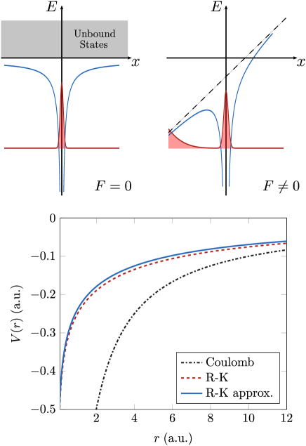
Figure 1: (Top) Electrostatic potential and wave functions of the LoSurdo-Stark effect. In the left panel the system is represented in the absence of the electric field and a bound state is formed. In the right panel an external electric field is superimposed on the attractive electrostatic field distorting the latter. Along one of the directions the total potential becomes more confining whereas in the opposite direction the external field creates a barrier through which the exciton can tunnel and thereby ionize. (Bottom) Comparison between the Coulomb potential and the two expressions defined in the text for the Rytova-Keldysh potential. While for large values of $r$ the potentials present an identical behaviour, for small $r$ a significant difference between the Coulomb and Rytova-Keldysh potentials is visible. Moreover, it is clear that the approximate expression for the Rytova-Keldysh potential gives an excellent approximation of Eq. (2). The parameters $\kappa=1$ and $r_{0}=10$ Å were used.

Following the steps of (Alexander, 1969; Damburg and Kolosov, 1978; Torres del Castillo and Morales, 2008) we will pass from polar to parabolic coordinates with the goal of decoupling the original two-variable differential equation into two one-dimensional differential equations. Unlike the pure Coulomb problem, this problem is not exactly separable. However, as will become apparent, this problem is separable under justifiable approximations.

In this work we are interested in studying the ionization rate of excitons in 2D materials due to an external static electric field. The Wannier equation in atomic units (a. u.) and in terms of the relative coordinate reads

$$\nabla^{2}\psi(\mathbf{r})-2\mu\left[-E+\mathbf{F\cdot r}+V(\mathbf{r})\right]\psi(\mathbf{r})=0,$$ (1)

where $\mu$ is the reduced mass of the electron-hole system, $E$ is the energy, and $\mathbf{F}=F\hat{x}$, with $F>0$, the external electric field, that we consider aligned along the $x$ direction. The electron-hole interaction $V(\mathbf{r})$ is given by the Rytova-Keldysh potential (Rytova, 1967; Keldysh, 1979)

$$V(\mathbf{r})=-\frac{\pi}{2r_{0}}\left[\mathbf{H}_{0}\left(\frac{\kappa r}{r_{0}}\right)-Y_{0}\left(\frac{\kappa r}{r_{0}}\right)\right],$$ (2)

where the so-called screening length $r_{0}$ is proportional to the polarizability of the 2D sheet Cudazzo et al. (2011). Macroscopically, it may be related to the thickness $d$ and dielectric function $\epsilon$ of the sheet as $r_{0}\sim d\epsilon/2$. Furthermore, $\kappa$ is the mean dielectric constant of the media above and below the 2D material, $\mathbf{H}_{0}$ is the Struve function, and $Y_{0}$ is the Bessel function of the second kind. The fact that the electrostatic interaction between electron-hole pairs in 2D materials is given by the Rytova-Keldysh potential is what gives rise to the nonHydrogenic Rydberg series (Chernikov et al., 2014). Inspired by the work of (Cudazzo et al., 2011), where an approximate expression for the Rytova-Keldysh potential is presented, we use the following expression as an approximation to Eq. (2)

$$V(\mathbf{r})\approx\frac{1}{r_{0}}\log\frac{\kappa r}{\kappa r+r_{0}}.$$ (3)

In Fig. 1 we plot Eq. (2) and the previous expression in the same graph and observe that the latter formula is an excellent approximation of the former.

Next we note that several authors (Alexander, 1969; Damburg and Kolosov, 1978; Torres del Castillo and Morales, 2008) used parabolic coordinates in order to separate the Schrödinger equation into two differential equations of a single variable. In those works, however, the Coulomb potential was considered in the 3D case. In our case, the Rytova-Keldysh potential does not allow a simple solution by separation of variables. To be able to do so, an effective potential has to be introduced. Let us consider the following set of parabolic coordinates (Sohnesen, 2016; Kamban and Christensen, 2018) in 2D:

$$x =\frac{\xi-\eta}{2},$$ (4)

$$y =\pm\sqrt{\xi\eta},$$ (5)

$$r =\frac{\xi+\eta}{2},$$ (6)

with both $\xi$ and $\eta$ belonging to the interval $[0,\infty[$. In these new coordinates the Laplacian reads

$$\nabla^{2}=\frac{4}{\eta+\xi}\left[\sqrt{\eta}\frac{\partial}{\partial\eta}\left(\sqrt{\eta}\frac{\partial}{\partial\eta}\right)+\sqrt{\xi}\frac{\partial}{\partial\xi}\left(\sqrt{\xi}\frac{\partial}{\partial\xi}\right)\right].$$ (7)

Applying this variable change to Eq. (1), and considering that $\psi(\eta,\xi)=v(\eta)u(\xi),$ we obtain an equation that can be separated, except for the potential term where $\xi$ and $\eta$ are still coupled by

$$\frac{(\eta+\xi)}{2}V\left(\frac{\eta+\xi}{2}\right).$$ (8)

To fully separate the $\xi$ and $\eta$ dependencies we propose the following effective potential

$$\frac{(\eta+\xi)}{2}V\left(\frac{\eta+\xi}{2}\right)\approx\frac{\eta}{2}V\left(\frac{\eta}{2}\right)+\frac{\xi}{2}V\left(\frac{\xi}{2}\right).$$ (9)

The reasoning behind this choice is as follows: we know that in the usual polar coordinates the Rytova-Keldysh potential obeys the following two limits

$$\lim_{r\rightarrow 0}rV(r) =0,$$ (10)

$$\lim_{r\rightarrow\infty}rV(r) =-\frac{1}{\kappa}.$$ (11)

It is therefore clear that the decoupling we have introduced respects the two previous limits. We have chosen the above separation for having asymptotically the Coulomb potential in both $\eta$ and $\xi$ coordinates. The quality of the approximation has to be judged by the accuracy of the formula for the ionization rate (anticipating the results, we find an excellent qualitative and quantitative agreement between the analytical results and the numerical ones). In view of the approximation made, the decoupled equations read

$$\left[\sqrt{\eta}\frac{\partial}{\partial\eta}\left(\sqrt{\eta}\frac{\partial}{\partial\eta}\right)+\frac{\mu E}{2}\eta-\frac{\mu}{2}\eta V\left(\frac{\eta}{2}\right)+\mu\frac{F}{4}\eta^{2}-Z\right]u(\eta) =0,$$ (12)

$$\left[\sqrt{\xi}\frac{\partial}{\partial\xi}\left(\sqrt{\xi}\frac{\partial}{\partial\xi}\right)+\frac{\mu E}{2}\xi-\frac{\mu}{2}\xi V\left(\frac{\xi}{2}\right)-\mu\frac{F}{4}\xi^{2}+Z\right]v(\xi) =0,$$ (13)

where $Z$ was introduced as a separation constant. Its value is determined below, demanding the correct large distance asymptotic behavior of the wave function. Using the proposed effective potential, the equations become mathematically identical, as they should, except for the external field term. Moreover, both equations reproduce the Coulomb problem in the asymptotic limit. We note that the two quantum problems defined in terms of the $\xi$ and $\eta$ coordinates have a completely different nature. While the $\xi-$equation defines a bound state problem, and is therefore tractable by simple methods, the $\eta-$equation defines a tunneling problem and obtaining its exact solution is challenging. These differential equations can be further simplified with the introduction of

$$u(\eta) =\frac{u_{1}(\eta)}{\eta^{1/4}},$$ (14)

$$v(\xi) =\frac{v_{1}(\xi)}{\xi^{1/4}},$$ (15)

which leads to

$$\left(\frac{d^{2}}{d\eta^{2}}+\frac{3}{16\eta^{2}}+\frac{\mu E}{2}-\frac{\mu}{2}V\left(\frac{\eta}{2}\right)+\frac{\mu F}{4}\eta-\frac{Z}{\eta}\right)u_{1}(\eta) =0$$ (16)

$$\left(\frac{d^{2}}{d\xi^{2}}+\frac{3}{16\xi^{2}}+\frac{\mu E}{2}-\frac{\mu}{2}V\left(\frac{\xi}{2}\right)-\frac{\mu F}{4}\xi+\frac{Z}{\xi}\right)v_{1}(\xi) =0.$$ (17)

As noted, solutions of these two equations at large distances from the origin have two different behaviors: the first one has an oscillatory behavior, whereas the second one decays exponentially. Furthermore, while the second equation has a discrete spectrum, the first has a continuous one. This is due to the different sign of the field term in the two equations.

Finally, to end this section, we introduce another change of variable that has already proven to be of great value in this type of problems, known as the Langer transformation (Langer, 1937; Good, 1953; Berry and de Almeida, 1973; Farrelly and Reinhardt, 1983), which is defined by

$$\eta =e^{t}\Rightarrow d\eta=e^{t}dt,$$ (18)

$$u_{1}(\eta) =e^{t/2}T(t).$$ (19)

Making use of this transformation, Eq. (16) acquires the form

$$T^{\prime\prime}(t)+P^{2}(t)T(t)=0,$$ (20)

with

$$P^{2}(t)=\frac{\mu E}{2}e^{2t}+\frac{\mu F}{4}e^{3t}-Ze^{t}-\frac{\mu}{2}V\left(\frac{e^{t}}{2}\right)e^{2t}-\frac{1}{16}$$ (21)

A similar transformation could be applied to Eq. (17). This, however, is not necessary. We note that the advantages of the above transformation are two-fold: on one side, the initial problem, valid only for $\eta\in[0,\infty[$, is transformed into a one-dimensional problem in the interval $t\in]-\infty,\infty[$, and on the other it removed the singular behavior at the origin due to the terms associated with $3/16\xi^{2}.$ As shown by Berry and Ozorio de Almeida (Berry and de Almeida, 1973), the Langer transformation is a key step in solving the 2D Hydrogen problem for zero angular momentum, which is similar to the problem at hands.

III Ionization Rate

In this section we will present a derivation for the ionization rate of excitons in 2D materials due to the external electric field. We will start by associating the ionization rate with an integral of the probability current density. This integral will contain the function $T(t)$, presented in the end of the previous section. Then, this function will be explicitly computed. Afterwards, combining the previous two steps, a fully analytical expression for the ionization rate will be presented.

III.1 The ionization rate formula

In the beginning of the text we considered the electric field to be applied along the $x$ direction, implying that the electrons will escape via the negative $x$ direction, which in the parabolic coordinates introduced in Eqs. (4)-(6) corresponds to large values of $\eta.$ Since the electrons will escape along the negative $x$ direction, we can define the ionization rate $W$ as (Bisgaard and Madsen, 2004)

$$W=-\int_{-\infty}^{\infty}j_{x}dy.$$ (22)

That is, the number of particles per unit time transversing a line perpendicular to the probability current density $j_{x},$ which reads

$$j_{x}=\frac{i}{2\mu}\left(\psi\frac{\partial\psi^{*}}{\partial x}-\psi^{*}\frac{\partial\psi}{\partial x}\right),$$ (23)

where, once again, $\mu$ is the reduced mass. In terms of parabolic coordinates, the position vector is

$$\mathbf{r}=\frac{\xi-\eta}{2}\hat{\mathbf{x}}+\sqrt{\xi\eta}\hat{\mathbf{y}}.$$ (24)

The differentials in Cartesian coordinates are related to the parabolic ones through the following relations

$$dx =\frac{1}{2}d\xi-\frac{1}{2}d\eta,$$ (25)

$$dy =\frac{1}{2}\sqrt{\frac{\eta}{\xi}}d\xi+\frac{1}{2}\sqrt{\frac{\xi}{\eta}}d\eta.$$ (26)

From here we find

$$\frac{\partial}{\partial x}=\frac{\partial\xi}{\partial x}\frac{\partial}{\partial\xi}+\frac{\partial\eta}{\partial x}\frac{\partial}{\partial\eta}\approx-2\frac{\partial}{\partial\eta},$$ (27)

where the final approximation comes from considering the limit $x\rightarrow-\infty$. Recalling what was done in the previous section we write

$$\psi(\eta,\xi) =u(\eta)v(\xi)$$ (28)

$$=\frac{u_{1}(\eta)}{\eta^{1/4}}\frac{v_{1}(\xi)}{\xi^{1/4}}.$$ (29)

Employing Eq. (19) this may also be written as

$$\psi(\eta,\xi)=\eta^{1/4}T\left[t(\eta)\right]\frac{v_{1}(\xi)}{\xi^{1/4}}.$$ (30)

The probability current density introduced in Eq. (23) can now be computed in parabolic coordinates as

$$j_{x}\approx\frac{i}{\mu}\sqrt{\eta}\frac{|v_{1}(\xi)|^{2}}{\xi^{1/2}}\left(T^{*}\frac{dT}{d\eta}-T\frac{dT^{*}}{d\eta}\right),$$ (31)

where, following the same reasoning as before, the derivatives in $\xi$ were ignored. Inserting this expression into Eq. (22) and approximating the differential in the $y$ coordinate by $dy\approx\sqrt{\eta/\xi}d\xi/2$ a generic expression for the ionization rate $W$ in 2D dimensions is obtained

$$W=-\frac{i}{\mu}\eta\left(T^{*}\frac{dT}{d\eta}-T\frac{dT^{*}}{d\eta}\right)\int_{0}^{\infty}\frac{|v_{1}(\xi)|^{2}}{\xi^{1/2}}d\xi.$$ (32)

Note the extra factor of $2$ picked up by the symmetric integral in Eq. (22). Having obtained this expression, we turn our attention to the computation of $T$.

III.2 Solution of the tunneling problem using a semiclassical method

To determine $T(t)$ we need to solve Eq. (20), which is so far fully equivalent to Eq. (16). In order to do so, we will use a uniform JWKB-type solution (where JWKB stands for Jeffrey-Wentzel-Kramers-Brillouin), known as the Miller and Good approach (Miller Jr and Good Jr, 1953; Berry and de Almeida, 1973). This method consists of introducing an auxiliary problem, whose solution is already established, to solve the main equation. The desired wave function will be given by the product of the solution to the auxiliary problem and a coordinate dependent amplitude. This amplitude consists of the quotient of two functions: in the denominator we have all the elements of the main equation associated with the non-differentiated term; in the numerator we have the analogous elements but for the auxiliary equation. This last term is the key difference between the Miller and Good approach and the usual JWKB method. While the latter leads to wave functions with divergences at the classical turning points, the former produces smooth wave functions across the whole domain. As the auxiliary problem that will help us solve Eq. (20), we introduce the Airy equation

$$\frac{d^{2}}{d\zeta^{2}}\phi(\zeta)+\zeta\phi(\zeta)=0,$$ (33)

whose solution reads

$$\phi(\zeta)=b_{2}\textrm{Ai}(-\zeta)+b_{1}\textrm{Bi}(-\zeta),$$ (34)

with $\textrm{Ai}(x)$ and ${\rm Bi}(x)$ the Airy functions. This equation has a single turning point at $\zeta=0$; the allowed and forbidden regions are located at $\zeta>0$ and $\zeta<0$, respectively. In order to have an outgoing wave in the propagating region we need to choose the coefficients $b_{1}$ and $b_{2}$ in a way that allows us to recover the correct asymptotic behavior. The asymptotic form of Eq. (34) reads

$$\phi(\zeta)\xrightarrow[\zeta\rightarrow\infty]{}b_{2}\frac{\sin\left[\frac{\pi}{4}+\frac{2}{3}\zeta^{3/2}\right]}{\sqrt{\pi}\zeta^{1/4}}+b_{1}\frac{\cos\left[\frac{\pi}{4}+\frac{2}{3}\zeta^{3/2}\right]}{\sqrt{\pi}\zeta^{1/4}}.$$ (35)

In order to obtain a traveling wave we choose $b_{2}=ib_{1}$; with this choice we obtain

$$\phi_{\textrm{out}}(\zeta)\sim b_{1}\frac{e^{i\frac{\pi}{4}+i\frac{2}{3}\zeta^{3/2}}}{\sqrt{\pi}\zeta^{1/4}},$$ (36)

as we desired. When $\zeta\rightarrow-\infty$ the solution Bi($-\zeta$) grows while $\textrm{Ai}(-\zeta)$ vanishes; thus, deep inside the forbidden region, we choose to approximate Eq. (34) by

$$\phi_{\textrm{forbidden}}(\zeta)\sim b_{1}\frac{e^{\frac{2}{3}(-\zeta)^{3/2}}}{\sqrt{\pi}(-\zeta)^{1/4}}.$$ (37)

Using these results we write the solution of (20) in the allowed region as

$$T\left[t(\eta)\right]=b_{1}\left(\frac{\zeta}{P^{2}(t)}\right)^{1/4}\frac{e^{i\frac{\pi}{4}+i\frac{2}{3}\zeta^{3/2}}}{\sqrt{\pi}\zeta^{1/4}},$$ (38)

with $P^{2}(t)$ given by Eq. (21) and $\zeta(t)$ is defined via the relation

$$\int_{0}^{\zeta}\sqrt{\zeta^{\prime}}d\zeta^{\prime}=\frac{2}{3}\zeta^{3/2}=\int_{t_{0}}^{t}\sqrt{P^{2}(t^{\prime})}dt^{\prime},$$ (39)

where $t_{0}$ corresponds to the classical turning point of $P^{2}(t)$, that is $P^{2}(t_{0})=0.$ Combining Eq. (39) with Eq. (38) it is easily shown that

$$T^{*}\frac{dT}{d\eta}-T\frac{dT^{*}}{d\eta}=\frac{2i}{\pi}\frac{|b_{1}|^{2}}{\eta},$$ (40)

which produces an ionization rate given by

$$W=\frac{|b_{1}|^{2}}{\pi\mu}\int_{0}^{\infty}\frac{|v_{1}(\xi)|^{2}}{\xi^{1/2}}d\xi.$$ (41)

Thus, to obtain $W$ two tasks remain: find $b_{1}$ and compute the integral in $\xi$. Let us now focus on the first one and only turn our attention to the second one later in the text.

III.3 Matching the wave function to an asymptotic one due to a Coulomb tail

In order to obtain $b_{1}$ we follow a conceptually simple procedure: we will determine the wave function $T\left[t(\eta)\right]$ deep inside the forbidden region, $-\infty\ll t\ll t_{0}$, in the limit of a small field $F$, and using the Miller and Good approach we will extract $b_{1}$ from the comparison of this equation with the asymptotic solution of the radial Wannier equation.

Once more, using the Miller and Good approach, but this time for the forbidden region, we write $T\left[t(\eta)\right]$ as

$$T(t)\sim\frac{b_{1}}{\sqrt{\pi}}\left[\frac{1}{-P^{2}(t)}\right]^{1/4}e^{\frac{2}{3}(-\zeta)^{3/2}}.$$ (42)

Note the sign differences between this equation and Eq. (38); these appear due to the different validity regions of the respective functions. In the limit of a weak field, $F\rightarrow 0$, we can approximate the $P^{2}(t)$ present in the denominator of the pre-factor with

$$-P^{2}(t)\approx-\frac{\mu E}{2}e^{2t}.$$ (43)

The function $\zeta$ is defined by the relation

$$\frac{2}{3}(-\zeta)^{3/2}=\int_{t}^{t_{0}}\sqrt{-P^{2}(t)}dt,$$ (44)

where once again $t_{0}$ denotes the zero of $P^{2}(t)$, and is approximately

$$t_{0}\sim\log\left(-\frac{2E}{F}\right).$$ (45)

To compute the integral in Eq. (44) we recall the form of $P^{2}(t)$ presented in Eq. (21) and discard the term $1/16$, since its contribution to the overall integral is insignificant. Then, we expand the integrand for small $\lambda,$ a book-keeping multiplicative parameter associated with the potential and the separation constant. Afterwards, we compute the integral, return to the original $\eta$ coordinate using the Langer transformation, and expand the result for small $F$ and large $\eta$, in this order. We note that the approximation presented in Eq. (43), although suitable for the pre-factor, is too crude to produce a reasonable result inside the integral. Now, the key step in this procedure, is the judicious choice of the separation constant $Z$; this is a degree of freedom we can take advantage of by choosing it as we desire. Accordingly, we choose $Z$ as

$$Z=\frac{\sqrt{-E\mu}}{2\sqrt{2}}.$$ (46)

This choice is made in order to allow us to recover a function with an $\eta$ dependence that matches the solution of the asymptotic differential equation for the Coulomb tail of the interaction potential. The wave function $u(\eta)$ is obtained from

$$u(\eta)=\eta^{1/4}T(t),$$ (47)

which can be written as

$$u(\eta) =b_{1}\frac{2^{1+\frac{3\sqrt{-E\mu}}{\sqrt{2}E\kappa}}e^{-\frac{2\sqrt{2}E\sqrt{-E\mu}}{3F}}}{\sqrt{\pi}\mu^{1/4}}(-E)^{\frac{\sqrt{-E\mu}}{\sqrt{2}E\kappa}}F^{-\frac{1}{4}-\frac{\sqrt{-E\mu}}{\sqrt{2}E\kappa}}$$

$$\times e^{-\frac{\eta\sqrt{-E\mu}}{\sqrt{2}}}\eta^{-\frac{1}{2}-\frac{\sqrt{-E\mu}}{\sqrt{2}E\kappa}}.$$ (48)

As briefly explained above, we now compare this wave function with the asymptotic solution for a particle (the exciton) of energy $E$ bound by a potential with a Coulomb tail. The asymptotic wave function in radial coordinates reads

$$\psi_{{\rm asympt}}(r) \sim Ae^{-r\sqrt{-2E\mu}}r^{\frac{\sqrt{2}\sqrt{\mu}-\sqrt{-E}\kappa}{2\sqrt{-E}\kappa}},$$ (49)

where $A$ is a constant determined from the normalization of the full wave function due to a Coulomb potential. Note that the wave function in parabolic coordinates reads $\psi(\eta,\xi)=u(\eta)v(\xi)$. In the ground state, and due to the symmetry of the equations defining both $u(\eta)$ and $v(\xi)$ in the absence of the field, we must have $u(\eta)=v(\eta)$. In the large $\eta$ limit, $\eta\gg\xi$, we find from Eq. (49) that $u(\eta)$ must be of the form

$$u(\eta)\sim\sqrt{A}e^{-\frac{\eta}{2}\sqrt{-2E\mu}}(\eta/2)^{\frac{\sqrt{2}\sqrt{\mu}-\sqrt{-E}\kappa}{2\sqrt{-E}\kappa}}$$ (50)

Comparing Eqs. (III.3) and (50) it follows that $b_{1}$ reads

$$b_{1} =\sqrt{A}\sqrt{\pi}\mu^{1/4}\frac{e^{\frac{2\sqrt{2}E\sqrt{-E\mu}}{3F}}}{F^{-\frac{1}{4}-\frac{\sqrt{-E\mu}}{\sqrt{2}E\kappa}}}2^{-\frac{1}{2}-2\frac{\sqrt{-2E\mu}}{2E\kappa}}(-E)^{-\frac{\sqrt{-2E\mu}}{2E\kappa}}.$$ (51)

Once $b_{1}$ has been determined, the remaining task is the calculation of the integral in the rate equation. Again, we take advantage of the Coulomb tail present in the potential binding the exciton. In this case, the radial wave function in a Coulomb potential, for a particle with energy $E$, reads

$$R(r)=Ae^{-\sqrt{-2E\mu}r}U\left(-\frac{\sqrt{2\mu}-\sqrt{-E}\kappa}{2\sqrt{-E}\kappa},1,2\sqrt{-2E\mu}r\right).$$ (52)

where $U(a,b,z)$ is the hypergeometric $U-$function. We now take $v(\xi)=A^{-1/2}R(\xi/2)$ and perform the integral. The result can be written as

$$\int_{0}^{\infty}\left|R(\xi/2)\right|^{2}\frac{d\xi}{\sqrt{\xi}}\equiv AA_{\xi}.$$ (53)

In general, it follows that the ionization rate $W$ reads

$$W =\frac{2}{\mu}A_{\xi}A^{2}\sqrt{\mu}\frac{e^{\frac{4\sqrt{2}E\sqrt{-E\mu}}{3F}}}{F^{-\frac{1}{2}-\frac{2\sqrt{-E\mu}}{\sqrt{2}E\kappa}}}2^{-1-4\frac{\sqrt{-2E\mu}}{2E\kappa}}(-E)^{-\frac{\sqrt{-2E\mu}}{E\kappa}},$$ (54)

and for the particular case of a 2D exciton bound by the Coulomb interaction we obtain

$$W=32\sqrt{\frac{2}{\pi}}\frac{\mu^{2}e^{-\frac{16\mu^{2}}{3F\kappa^{3}}}}{\sqrt{F}\kappa^{7/2}},$$ (55)

a result identical to that found by Tanaka et al. (Tanaka et al., 1987). In general, for any potential with a Coulomb tail we find

$$W=g_{0}^{2}W_{0}(F),$$ (56)

where

$$W_{0}(F)=\frac{e^{\frac{4\sqrt{2}E\sqrt{-E\mu}}{3F}}}{F^{-\frac{1}{2}-\frac{2\sqrt{-E\mu}}{\sqrt{2}E\kappa}}},$$ (57)

and

$$g_{0}^{2}\approx\frac{\kappa 2^{\frac{2\sqrt{2}\mu}{\kappa\sqrt{-E\mu}}+\frac{5}{4}}(-E){}^{\frac{\sqrt{2}\mu}{\kappa\sqrt{-E\mu}}+\frac{5}{4}}\Gamma\left(\frac{\sqrt{2}\mu}{\kappa\sqrt{-E\mu}}-\frac{1}{2}\right)}{\pi\sqrt[4]{\mu}\Gamma\left(\frac{\sqrt{2}\mu}{\kappa\sqrt{-E\mu}}\right)}$$ (58)

where $\Gamma(z)$ is the gamma function. Equation (56) together with Eq. (58) are the central results of this paper. Special limits of this last result can be obtained for carefully chosen values of $E$, $\kappa$, and $\mu$. In particular, for $E$ given by $E=-2\mu/\kappa^{2}$, corresponding to the ground state energy of a 2D exciton bound by the Coulomb potential, we recover the result given by Eq. (55) for the rate $W$. In the next section we explore the consequences of Eqs. (56) and (54).

IV Results

Having determined the form of the ionization rate, we can compare our results with numerical ones obtained via the solution of an eigenvalue problem for the exciton’s motion using the complex scaling method, which allow us to access complex eigenvalues, with the imaginary part interpreted as the rate $W$ computed above. Below we give a brief account of how the numerical calculations are performed.

IV.1 Complex scaling method

When a system that may be ionized is subjected to an external electric field, the energy eigenvalue turns complex. The ionization rate of the system is then described by the imaginary part of the energy as $\Gamma=-2\mathrm{Im}\,E$. A formally exact method of computing the complex energy is to transform the original eigenvalue problem into a non-hermitian eigenvalue problem via the complex scaling technique Balslev and Combes (1971); Aguilar and Combes (1971); Herbst and Simon (1978); Reed and Simon (1982). Here, one rotates the radial coordinate into the complex plane by an angle $\phi$ to circumvent the diverging behavior of the resonance states Ho (1983). The method is incredibly flexible, and one may choose to either rotate the entire radial domain as $r\to re^{i\phi}$ or choose to only rotate the coordinate outside a desired radius $R$ as

$$r\to\begin{cases}r\quad&\mathrm{for}\,\,r<R\\ R+\left(r-R\right)e^{i\phi}\quad&\mathrm{for}\,\,r>R\thinspace.\end{cases}$$ (59)

The latter, so-called exterior complex scaling (ECS) technique, was first introduced because the uniform complex scaling (UCS) technique was not applicable within the Born-Oppenheimer approximation Simon (1979). When both methods may be applied to the same potential, which is the case for all potentials considered here, they yield identical eigenvalues. UCS is easier to implement, and has been used to obtain ionization rates of excitons in monolayer MoS₂ Haastrup et al. (2016) and WSe₂ Mas (2018) for relatively large fields. However, the ECS technique Simon (1979); Scrinzi and Elander (1993) is much more efficient for the weak fields that are relevant for excitons in 2D semiconductors Kamban and Pedersen (2019). Using the contour defined by Eq. (59) in the eigenvalue problem, we obtain states that behave completely differently in the interior $r<R$ and exterior $r>R$ domains. Furthermore, there are discontinuities at $R$ that we have to deal with Scrinzi and Elander (1993); Scrinzi (2010). An efficient method of solving these types of problems is to use a finite element basis to resolve the radial behavior of the states. To this end, we divide the radial domain into $N$ segments $\left[r_{n-1},r_{n}\right]$. A set of $p$ functions satisfying

$$f_{i}^{\left(n\right)}\left(r_{n-1}\right)=f_{i}^{\left(n\right)}\left(r_{n}\right)=0\thinspace,$$

$$\mathrm{except}\quad f_{1}^{\left(n\right)}\left(r_{n-1}\right)=f_{p}^{\left(n\right)}\left(r_{n}\right)=1\thinspace,$$ (60)

is then introduced on each segment $n$ in order to make enforcing continuity across the segment boundaries simple. In practice, we transform the Legendre polynomials such that they satisfy Eq. (60) Scrinzi (2010). The wave function may then be written as

$$\psi\left(\boldsymbol{r}\right)=\sum_{m=0}^{M}\sum_{n=1}^{N}\sum_{i=1}^{p}c_{i}^{\left(m,n\right)}f_{i}^{\left(n\right)}\left(r\right)\cos\left(m\theta\right)\thinspace,$$ (61)

where continuity across the segment boundaries is ensured by enforcing

$$c_{p}^{\left(m,n-1\right)}=c_{1}^{\left(m,n\right)}\thinspace,\quad n=2,...,N\thinspace,$$ (62)

in the expansion coefficients. As the unperturbed problems considered here are radially symmetric, an efficient angular basis of cosine functions may be used to resolve the angular behavior of the states. Using this expansion, the Wannier equation may be transformed into a matrix eigenvalue problem and solved efficiently using techniques for sparse matrices. Note that we keep the radial coordinate in the basis functions real and leave it to the expansion coefficients to describe the behavior along the complex contour. This technique has previously been used to compute ionization rates of excitons in monolayer semiconductors Kamban and Pedersen (2019) as well as bilayer heterostructures Kamban and Pedersen (2020), and we shall use it here to validate the analytical results.

IV.2 An application

To illustrate the validity of our analytical formula over a significant range of values of the external field $F$, we compute the ionization rate for excitons in the 2D Hydrogen atom, hBN, WSe₂ and MoS₂. In previous publications we have shown that excitons in hBN and TMDs are well described by the Wannier equation with the Rytova-Keldysh potential (Ferreira et al., 2019; Henriques et al., 2020a). In Fig. 2 we present a comparison of our analytical results with the finite element method (FEM) approach described above. There is a remarkable agreement between both approaches across the four cases of study. The analytical results excel at moderate and small field values, but start to deviate from the exact numerical methods at extremely large fields. This is to be expected, since our analytical result was obtained in the limit of small fields. At very small fields the FEM struggles to give accurate results, a region where the analytical approach is highly accurate. Moreover, the FEM requires time-expensive calculations and convergence needs to be confirmed for every case. Needless to say, the analytical approach suffers not from these two shortcomings. Also, the analytical approach makes studying the dependence on the dielectric environment surrounding the 2D material (Chaves et al., 2017) easy.

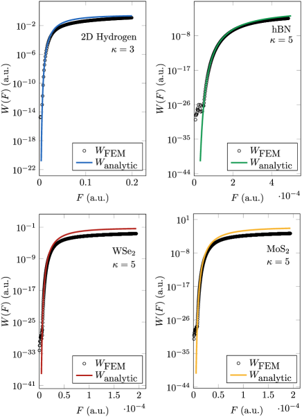
Figure 2: Comparison of the numerical and analytical calculation of the rate for hBN excitons. The reduced mass of the exciton in H, hBN, MoS₂, WSe₂ is $\mu=1,\,0.5,\,0.28,\,0.23$, respectively, the parameters describing the polarizability of hBN, MoS₂, WSe₂ is $r_{0}=10,\,43.4,\,46.2$ Å, respectively, and the dielectric constants is $\kappa=5$ for all but Hydrogen, for which $\kappa=3$. All quantities depicted are given in atomic units (a. u.) and the parameters were taken from Ref. (Kamban and Pedersen, 2019).

V Final remarks

In this paper we have derived an expression for the ionization rate of excitons in a 2D material due to the application of an external static electric field. Our result is quantitatively accurate, as was shown in the bulk of the text. Our approach took a semi-classical path, based on an approximate separation of the Rytova-Keldysh potential in parabolic coordinates. This step is key in the derivation, and is justifiable on the basis of the behavior of the potential near the origin and at large distances. The next key step is the solution of a tunneling problem, described by one of the equations arising from the separability procedure, the $\eta-$equation. The solution of the tunneling problem was achieved via a uniform semi-classical method, developed by Miller and Good and used by Berry and Ozorio de Almeida for the 2D Coulomb problem, for zero angular momentum channel. Once the semi-classical solution is found, we match it with the asymptotic solution of a particle of reduced mass $\mu$ (the exciton reduced mass) and energy $E$, in a dielectric environment characterized by a dielectric function $\kappa$, in a Coulomb potential. This matching requires that the original potential binding the electron and hole has a Coulomb tail, which is fortunately true in our case. Therefore, for every potential with a Coulomb tail our method is applicable. One advantage of the method, besides giving an analytical solution for the ionization rate, is that it is easily extendable to other classes of potentials such as those discussed by Pfeiffer (Pfeiffer et al., 2012). Finally, we note that our result can be extended to the calculation of the photo-ionization rate of the exciton due to an external electric field of frequency $\omega$. To achieve this, we replace the electric field strength by $F(t)=F_{0}\cos(\omega t)$ in the rate equation and average over one cycle. Although this procedure is not exact, it should give good results in the low frequency regime.