Sensitivity Reach on the Heavy Neutral Leptons and $\tau$-Neutrino Mixing $|U_{\tau N}|^{2}$ at the HL-LHC

Abstract

The model of heavy neutral leptons (HNLs) is one of the well-motivated models beyond the standard model from both theoretical and phenomenological point of views. It is an indispensable ingredient to explain the puzzle of tiny neutrino masses and the origin of the matter-antimatter asymmetry in our Universe, based on the models in which the simplest Type-I seesaw mechanism can be embedded. The HNL with a mass up to the electroweak scale is an attractive scenario which can be readily tested in present or near-future experiments including the LHC. In this work, we study the decay rates of HNLs and find the sensitive parameter space of the mixing angles between the active neutrinos and HNLs. Since there are fewer collider studies of the mixing between $\nu_{\tau}$ and HNL in literature compared with those of $\nu_{e}$ and $\nu_{\mu}$ for the HNL of mass in the electroweak scale, we focus on the channel $pp\rightarrow W^{\pm(\ast)}+X\rightarrow\tau^{\pm}N+X$ to search for HNLs at the LHC 14 TeV. The targeted signature consists of three prompt charged leptons, which include at least two tau leptons. After the signal-background analysis, we further set sensitivity bounds on the mixing $|U_{\tau N}|^{2}$ with $M_{N}$ at High-Luminosity LHC (HL-LHC). We predict the testable bounds from HL-LHC can be stronger than the previous LEP constraints and Electroweak Precision Data (EWPD), especially for $M_{N}\lesssim$ 50 GeV can reach down to $|U_{\tau N}|^{2}\approx 5\times 10^{-6}$.

I Introduction

Neutrino oscillation is one of the definite evidences of physics beyond the standard model, which implies that at least two of three active neutrinos are massive. However, there is no clear answer for the origin of neutrino-mass generation. Further, the matter-antimatter asymmetry in our Universe is another mystery that the SM cannot explain. To address these problems the conventional Type-I seesaw mechanism Minkowski:1977sc ; Yanagida:1979as ; Yanagida:1980xy ; GellMann:1980vs ; Ramond:1979 ; Glashow:1979 ; Mohapatra:1979ia with at least two superheavy right-handed neutrinos is one of the the simplest possibilities and widely discussed so far. Thanks to the existence of heavy Majorana neutrinos, the observed tiny neutrino masses are naturally explained and their decays can be the source of the baryon asymmetry of the Universe (BAU) through a well-known mechanism called thermal leptogenesis Fukugita:1986hr .

Hence, if heavy Majorana neutrinos are discovered, it would be a clear signal of new physics without any doubts. Unfortunately, since the thermal leptogenesis requires the scale of the Majorana neutrinos to be superheavy, say more than $10^{9}~{}{\rm GeV}$ Davidson:2002qv , and the conventional Type-I seesaw can be perturbatively applied up to around the GUT scale, $10^{15}~{}{\rm GeV}$, we cannot directly produce and test such heavy particles in near-future terrestrial experiments. However, this is not the end of the story because the allowed mass range for the heavy Majorana neutrinos can be very wide below the GUT scale. On the other hand, once the mass of the heavy Majorana neutrinos, which contribute to the seesaw mechanism, becomes below the pion mass in the minimal model, it would conflict with the constraints from the Big Bang Nucleosynthesis, since its lifetime becomes longer than 1 sec Ruchayskiy:2012si . Therefore, the Type-I seesaw mechanism itself can be valid for the mass range of right-handed neutrinos between $\sim\mathcal{O}(100~{}{\rm MeV})$ and the GUT scale.

Among a bunch of possibilities, the one with heavy Majorana neutrinos below the electroweak scale is an attractive scenario which can be readily tested in present or near future experiments. A model called the Neutrino Minimal Standard Model ($\nu$MSM) Asaka:2005an ; Asaka:2005pn , in which the SM is extended only by introducing three heavy Majorana neutrinos, possesses two such neutrinos around the electroweak scale and one in the keV scale which also serves as a dark matter candidate. Since the neutrino Yukawa coupling of the keV-scale Majorana neutrino is so tiny compared with the other two that we can completely separate its physics from the others and simply focus on the dynamics of the other two heavier Majorana neutrinos, namely, the contribution from the keV-scale Majorana neutrino to the seesaw neutrino mass is small enough and the lightest active neutrino mass is suppressed enough compared with the solar neutrino mass scale. The other two Majorana neutrinos, which have the mass above the pion mass and below the EW scale, are responsible for the explanations of the observed atmospheric and solar neutrino mass scales and baryogenesis via neutrino oscillation Akhmedov:1998qx ; Asaka:2005pn .

Generically, the mass eigenstates of the heavy Majorana neutrinos are called heavy neutral leptons (HNLs) and labeled as $N$. The HNLs can be searched for at terrestrial experiments and, especially the testability at beam dump experiments where bunches of kaon and B mesons are produced when HNLs are lighter than the parent mesons as firstly proposed by Shrock:1980vy ; Shrock:1980ct ; Shrock:1981wq (see e.g. Atre:2009rg ; Asaka:2011pb ; Asaka:2016rwd ; Abada:2019bac ; Chun:2019nwi ; Bryman:2019bjg for recent relevant works). Furthermore, the HNLs can also be searched for at colliders like the LHC as well and searchable range of HNL mass becomes wider than the beam damp experiments (see e.q. Kersten:2007vk ; Atre:2009rg ; Blondel:2014bra ; Deppisch:2015qwa ; Drewes:2016jae ; Cai:2017mow ; Helo:2018qej ; Liu:2019qfa and references therein). Actually, the lepton-number-violating (LNV) channels are the most specular signals and the definite discriminator of the models because the HNLs uniquely break lepton number which the SM always preserves. Not only for that but the lepton-number-conserving (LNC) channels can also provide strong hints for searching for the HNLs.

Although the mixing between $\nu_{\tau}$ and HNL is more challenging to be probed compared with those of $\nu_{e}$ and $\nu_{\mu}$, there already exist some studies for $M_{N}\sim\mathcal{O}(1\mathchar 45\relax 5)$ GeV in Ref. Bondarenko:2018ptm ; Cvetic:2019shl , $M_{N}\sim\mathcal{O}(1\mathchar 45\relax 20)$ GeV in Refs. Abada:2018sfh ; Cottin:2018nms ; Hernandez:2018cgc ; Drewes:2019vjy , and $M_{N}>150$ GeV in Ref. Andres:2017daw ; Pascoli:2018rsg . However, for $25<M_{N}<150$ GeV, the detectability of the mixing between $\nu_{\tau}$ and HNL is not well-studied at the LHC. In this work, we focus on the channel $pp\rightarrow W^{\pm(\ast)}+X\rightarrow\tau^{\pm}N+X$ to search for HNLs with $25<M_{N}<150$ GeV at the High-Luminosity LHC (HL-LHC). In this work, we focus on the channel $pp\rightarrow W^{\pm(\ast)}+X\rightarrow\tau^{\pm}N+X$  to search for HNLs with $25<M_{N}<150$ GeV at the High-Luminosity LHC (HL-LHC). Our characteristic signature consists of three prompt charged leptons, where at least two tau leptons are included. With a detailed signal-background analysis we can set sensitivity bounds on the mixing angle $|U_{\tau N}|^{2}$ with $M_{N}$ at the HL-LHC. Especially, it can be improved by a factor of five over the previous analyses when $M_{N}\lesssim 50~{}{\rm GeV}$. This is a significant improvement over previous studies.

The organization of the paper is as follows. We highlight some details of the model that are relevant to our study and calculate the decay rates of HNLs in Sec. II. In Sec. III, we survey the valid parameter space for the mixing of the active neutrinos with HNLs in various HNL mass ranges up to the electroweak scale. In Sec. IV, we give details about the search for HNL with $\tau$ leptons at the HL-LHC. In Sec. V, we present the signal-background analysis and the results, and obtain the sensitivity bounds on the mixing $|U_{\tau N}|^{2}$. We conclude in Sec. VI.

II The Neutrino Minimal Standard Model

II.1 The model

In this section, we highlight some details of the Neutrino Minimal Standard Model ($\nu$MSM) which are relevant to our study. After introducing three gauge-singlet right-handed neutrino fields into the SM, the total Lagrangian can be written as

$$\mathcal{L}=\mathcal{L}_{\rm SM}+i\,\overline{\nu_{RI}}\gamma^{\mu}\partial_{\mu}\nu_{RI}-\left(F_{\alpha I}\,\overline{\ell_{\alpha}}\,\Phi\,\nu_{RI}+\frac{M_{I}}{2}\,\overline{\nu_{RI}^{c}}\,\nu_{RI}+h.c.\right)\,,$$ (1)

where $\mathcal{L}_{\rm SM}$ is the SM Lagrangian based on $SU(3)_{c}\times SU(2)_{L}\times U(1)_{Y}$ gauge symmetry, the index $\alpha$ denotes the active flavors running for $e,\mu,$ and $\tau$, and $I$ is the HNL-flavor index running from $1$ to $3$. The fields $\ell$, $\Phi$, and $\nu_{R}$ are the lepton doublet, the Higgs doublet, and the right-handed neutrino singlet, respectively. $F_{\alpha I}$’s are the neutrino Yukawa coupling constants and $M_{I}$’s are the Majorana masses for the right-handed neutrinos.

After the Higgs field acquires the vacuum expectation value, there are two kinds of neutrino masses, namely, the Dirac neutrino masses defined as $(M_{D})_{\alpha I}\equiv F_{\alpha I}\langle\Phi\rangle$ and the Majorana neutrino masses, $M_{I}$. In the mass basis of neutrinos, the tiny active neutrino masses can be explained by the hierarchical ratio between Dirac and Majorana masses as $M_{D}^{2}/M_{I}$ realized by the seesaw mechanism. In the mass basis, the HNLs are composed of mostly right-handed neutrinos but also small portion of left-handed neutrinos, thus, HNLs can have gauge interactions through the mixing denoted as $U_{\alpha I}\equiv(M_{D})_{\alpha I}/M_{I}$. Therefore, HNLs can be searched for at terrestrial experiments.

As discussed in a number works in literature  (see e.g. Chun:2017spz and references therein and also related papers) a certain amount of mass degeneracy between two HNLs is necessary for the success of baryogenesis. Then, we can simply rewrite the Majorana masses as $M_{2,3}=M_{N}\pm\Delta M/2$ where $M_{N}$ is the common mass and $\Delta M$ denotes the slight mass difference. We do not stick ourselves to the valid parameter space for baryogenesis in the following studies, though. Between these two mass parameters, the common mass scale is more important than their slight difference for the purpose of HNLs searches since $\Delta M/M\ll 1$. Therefore, we can safely neglect the correction of $\Delta M$ and simply multiply a factor of 2 when we want to estimate physical observables, such as cross sections, for HNLs in the $\nu$MSM. In the following analyses and discussion, however, we focus on the case with one HNL just for simplicity and denote the mixing angle as $U_{\alpha N}$.

II.2 Decay rates of the Heavy Neutral Leptons

Based on the mass range of HNLs, we can calculate its decay rate in three mass ranges: (1) low mass region ($M_{N}\ll m_{W,Z}$), (2) medium mass region ($M_{N}\lesssim m_{t}$) and (3) high mass region ($M_{N}\gg m_{W,Z}$). Here we only focus on the low and medium mass ranges in this study.

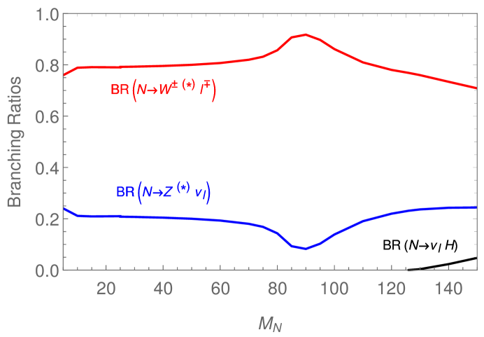
Figure 1: The branching ratios of the HNL with the assumption $|U_{eN}|^{2}=|U_{\mu N}|^{2}=|U_{\tau N}|^{2}$ for the decay modes $N\rightarrow W^{\pm(\ast)}l^{\mp}_{\alpha}$, $N\rightarrow Z^{(\ast)}\nu_{\alpha}$ and $N\rightarrow\nu_{\alpha}H$ of HNL in the low and medium mass regions.

In the low and medium mass ranges of HNL, the major decay modes are $N\rightarrow W^{\pm(\ast)}l^{\mp}_{\alpha}$ and $N\rightarrow Z^{(\ast)}\nu_{\alpha}$, where $W,Z$ bosons can be either on-shell or off-shell depending on $M_{N}$. Once HNL is heavier than the Higgs boson, the $N\rightarrow\nu_{\alpha}H$ decay mode is also open. All detailed formulas for these partial decay widths are collected in Appendix A. The branching ratios with the assumption $|U_{eN}|^{2}=|U_{\mu N}|^{2}=|U_{\tau N}|^{2}$ for the above decay modes of HNL in the above mass ranges are shown in Fig. 1. Since $BR(N\rightarrow W^{\pm(\ast)}l^{\mp}_{\alpha})$ is dominant for the whole mass range, we focus on $N\rightarrow W^{\pm(\ast)}l^{\mp}_{\alpha}$ in the following study.

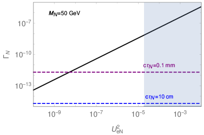
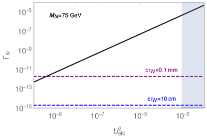
Figure 2: The decay width $\Gamma_{N}$ versus the mixing parameter $U^{2}_{eN}$ (solid line) in the parameter space of ($U^{2}_{eN}$, $\Gamma_{N}$) with $M_{N}$ = $5$ GeV (upper-left), $25$ GeV (upper-right), $50$ GeV (lower-left) and $75$ GeV (lower-right). The shaded regions come from various constraints shown in Fig. 4. The three dashed lines indicate the benchmark decay lengths of $c\tau_{N}$ = $0.1$ mm (purple), $10$ cm (blue) and $10$ m (brown).

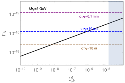
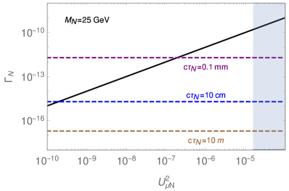
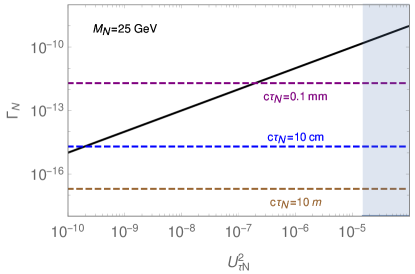
Figure 3: The decay width $\Gamma_{N}$ versus the mixing parameter $U^{2}_{\mu N}$ (upper panels) or $U^{2}_{\tau N}$ (lower panels) in the parameter space of ($U^{2}_{\mu N}$, $\Gamma_{N}$) with $M_{N}$ = $5$ GeV (upper-left) and $25$ GeV (upper-right), and of ($U^{2}_{\tau N}$, $\Gamma_{N}$) with $M_{N}$ = $5$ GeV (lower-left) and $25$ GeV (lower-right). The shaded regions come from various constraints shown in Fig. 5 and Fig. 6, respectively. The three dashed lines indicate the benchmark decay lengths of $c\tau_{N}$ = $0.1$ mm (purple), $10$ cm (blue) and $10$ m (brown).

The dependence of the total decay rate $\Gamma_{N}$ on the square of mixing parameter $U^{2}_{\alpha N}$ ($\alpha=e,\mu,\tau$) is numerically studied below. We first show $\Gamma_{N}$ verse $U^{2}_{eN}$ with $M_{N}$ = $5$, $25$, $50$ and $75$ GeV in Fig. 2. Since we ignore the fermion mass in the final state for the medium mass range in our numerical calculations, there is no difference among the lepton flavors in this mass range. We show $\Gamma_{N}$ verse $U^{2}_{\mu N}$ and $\Gamma_{N}$ verse $U^{2}_{\tau N}$ with only $M_{N}$ = $5$ and $25$ GeV in Fig. 3. The shaded regions come from the constraints shown in Figs. 4 to 6 in the next section. Three dashed lines indicate the benchmark decay lengths of $c\tau_{N}$ = $0.1$ mm (purple), $10$ cm (blue) and $10$ m (brown). We observe that once $M_{N}\gtrsim$ $50$ GeV and $U^{2}_{\alpha N}\gtrsim 10^{-8}$, the decay length of HNL is quite small such that we can simply take the decay of HNL as prompt in most of the parameter space for each lepton flavor. In contrast, the low mass HNL with tiny $U^{2}_{\alpha N}$ can easily generate the displaced vertex signature after it has been produced at colliders Alekhin:2015byh ; Kling:2018wct ; Curtin:2018mvb ; Lee:2018pag ; Abada:2018sfh ; Dercks:2018wum ; Alimena:2019zri ; Aielli:2019ivi ; Hirsch:2020klk , which is of immense interest in the upcoming LHC run.

III Constraints for Heavy Neutral Leptons

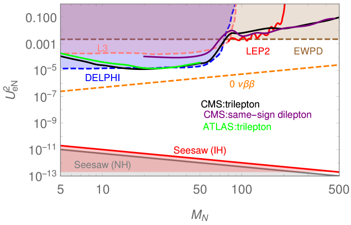
Figure 4: The allowed parameter space of ($M_{N}$, $|U_{eN}|^{2}$). We display the main constraints from EWPD delAguila:2008pw ; Akhmedov:2013hec ; Basso:2013jka ; deBlas:2013gla ; Antusch:2015mia (brown dashed line), L3 Adriani:1992pq ; Acciarri:1999qj ; Achard:2001qv (pink dashed line), DELPHI Abreu:1996pa (blue dashed line), LEP2 Adriani:1992pq ; Acciarri:1999qj ; Achard:2001qv (red solid line), CMS-13TeV trilepton Sirunyan:2018mtv (black solid line), CMS-13TeV same-sign dilepton Sirunyan:2018xiv ( purple solid line), ATLAS-13TeV trilepton Aad:2019kiz (green solid line), $0\nu\beta\beta$ (orange dashed line) and Seesaw (NH) (Seesaw(IH)) (gray solid line (red solid line)) on the plane.

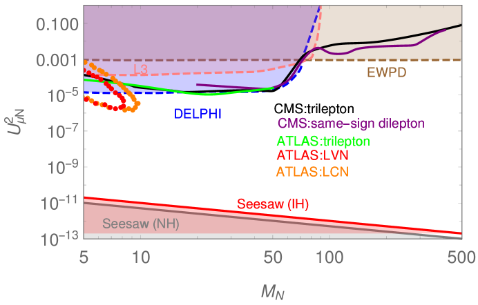
Figure 5: The allowed parameter space of ($M_{N}$, $|U_{\mu N}|^{2}$). We display the main constraints from EWPD delAguila:2008pw ; Akhmedov:2013hec ; Basso:2013jka ; deBlas:2013gla ; Antusch:2015mia (brown dashed line), L3 Adriani:1992pq ; Acciarri:1999qj ; Achard:2001qv (pink dashed line), DELPHI Abreu:1996pa (blue dashed line), CMS-13TeV trilepton Sirunyan:2018mtv (black solid line), CMS-13TeV same-sign dilepton Sirunyan:2018xiv (purple solid line), ATLAS-13TeV trilepton, LVN and LCN Aad:2019kiz (green solid line, red dotted line and orange dotted line) and Seesaw (NH) (Seesaw(IH)) (gray solid line (red solid line)) on the plane.

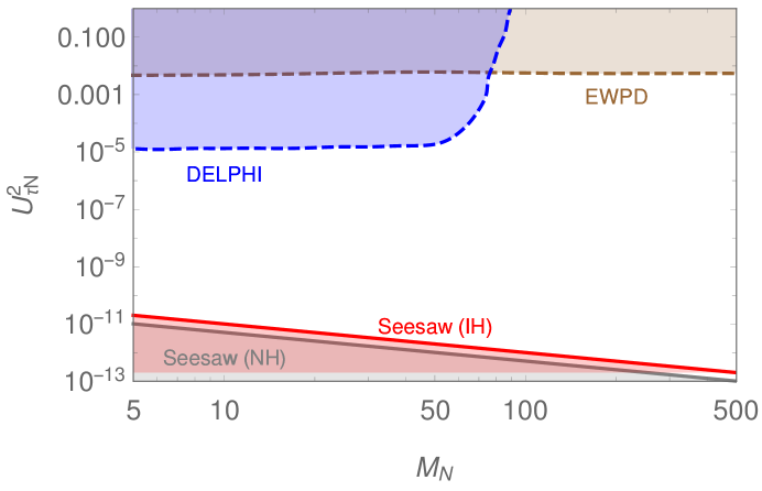
Figure 6: The allowed parameter space of ($M_{N}$, $|U_{\tau N}|^{2}$). We display the main constraints from EWPD delAguila:2008pw ; Akhmedov:2013hec ; Basso:2013jka ; deBlas:2013gla ; Antusch:2015mia (brown dashed line), DELPHI Abreu:1996pa (blue dashed line) and Seesaw (NH) (Seesaw(IH)) (gray solid line (red solid line)) on the plane.

In this section, we summarize various constraints on the mixing $|U_{\alpha N}|^{2}$ ($\alpha=e,\mu,\tau$) in the mass range of $M_{N}$ from $5$ to $500$ GeV. We categorize these constraints as follows.

1. Electroweak Precision Data (EWPD) delAguila:2008pw ; Akhmedov:2013hec ; Basso:2013jka ; deBlas:2013gla ; Antusch:2015mia ,

2. Large Electron–Positron (LEP) Collider experiments, including L3 Adriani:1992pq ; Acciarri:1999qj ; Achard:2001qv , DELPHI Abreu:1996pa , and LEP2 Adriani:1992pq ; Acciarri:1999qj ; Achard:2001qv ,

3. Large Hadron Collider (LHC) experiments, including CMS-13TeV trilepton Sirunyan:2018mtv , CMS-13TeV same-sign dilepton Sirunyan:2018xiv and ATLAS-13TeV trilepton Aad:2019kiz ,

4. Neutrinoless double beta ($0\nu\beta\beta$) decay, and

5. Theoretical lower bound of the seesaw mechanism.

We first show the valid parameter space of ($M_{N}$, $|U_{eN}|^{2}$) in Fig. 4. Generally, $|U_{eN}|^{2}\lesssim 2\times 10^{-5}$ for $M_{N}\lesssim 50$ GeV. The main constraints for this mass region come from DELPHI Abreu:1996pa , CMS-13TeV trilepton Sirunyan:2018mtv and ATLAS-13TeV trilepton searches Aad:2019kiz . On the other hand, $|U_{eN}|^{2}\lesssim 2.2\times 10^{-3}$ for $M_{N}\gtrsim 100$ GeV from constraints of LEP2 Adriani:1992pq ; Acciarri:1999qj ; Achard:2001qv and EWPD delAguila:2008pw ; Akhmedov:2013hec ; Basso:2013jka ; deBlas:2013gla ; Antusch:2015mia . The jump of the $|U_{eN}|^{2}$ constraints from $M_{N}\approx 50$ to $100$ GeV comes from the threshold of gauge boson masses $m_{W,Z}$. In addition, we follow Eq. (2.18) in Ref. Atre:2009rg for the constraint of $0\nu\beta\beta$ decay which is the strongest in Fig. 4.

Similarly, the valid parameter space of ($M_{N}$, $|U_{\mu N}|^{2}$) is shown in Fig. 5. Again, $|U_{\mu N}|^{2}\lesssim 2\times 10^{-5}$ for $M_{N}\lesssim 50$ GeV, but $|U_{\mu N}|^{2}\lesssim 9\times 10^{-4}$ for $M_{N}\gtrsim 100$ GeV. Interestingly, the search for displaced-vertex signature of muons from HNL in the case of lepton-number violation (LNV) and lepton-number conservation (LNC) was published in Ref. Aad:2019kiz from the ATLAS Collaboration. The above searches set a stronger constraint for $M_{N}<10$ GeV.

Finally, we show the valid parameter space of ($M_{N}$, $|U_{\tau N}|^{2}$) in Fig. 6. The main constraints only come from EWPD delAguila:2008pw ; Akhmedov:2013hec ; Basso:2013jka ; deBlas:2013gla ; Antusch:2015mia and DELPHI Abreu:1996pa with $|U_{\tau N}|^{2}\lesssim 5.5\times 10^{-3}$ for $M_{N}\gtrsim 100$ GeV.

We observe that the constraints on the mixing between $\nu_{\tau}$ and HNLs are relatively weaker than both $\nu_{e}$ and $\nu_{\mu}$ in the electroweak scale HNLs. On the other hand, we approximately apply the $m_{3}$ value of Normal Hierarchical (NH) case and $m_{2},m_{1}$ values of Inverted Hierarchical (IH) case from PDG 2018 Tanabashi:2018oca , respectively, to set the theoretical lower bound of the seesaw mechanism for the mixing angles ($M_{N}$, $|U_{\alpha N}|^{2}$) in Figs. 4 to 6.

IV Search for the HNL with $\tau$ lepton at HL-LHC

To our knowledge there have not been any concrete analyses for the sensitivity reach of $U^{2}_{\tau N}$ for HNLs around the EW scale at the LHC. Here we propose to search for HNLs with the signatures consisting of three prompt charged leptons in the final state, of which at least two are tau leptons. We first study the kinematical behavior of the HNL in the production channel, $pp\rightarrow W^{\pm(\ast)}+X\rightarrow\tau^{\pm}N+X$, and then discuss the signatures for various final states from the HNL decays and discuss possible SM backgrounds. Finally, the details of simulations and event selections for both signals and SM backgrounds are displayed.

IV.1 Kinematical behavior of the HNL in the production channel $pp\rightarrow W^{\pm(\ast)}+X\rightarrow\tau^{\pm}N+X$

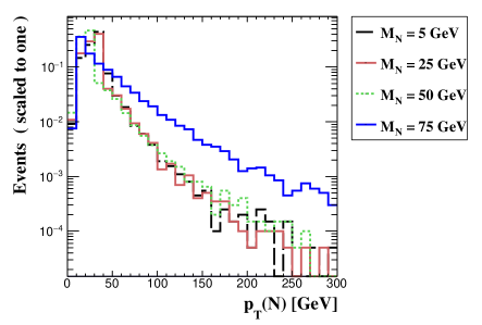
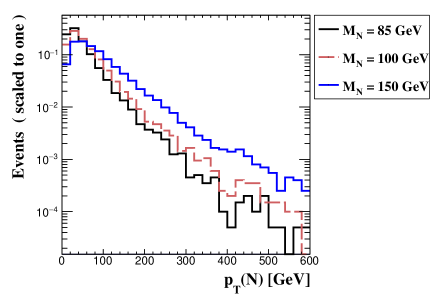
Figure 7: The transverse momentum $p_{T}(N)$ distribution of the HNL in the process $pp\rightarrow W^{\pm(\ast)}\rightarrow\tau^{\pm}N+X$ at $\sqrt{s}=14$ TeV for some benchmark points with $M_{N}<m_{W}$ (left) and $M_{N}>m_{W}$ (right) at parton level.

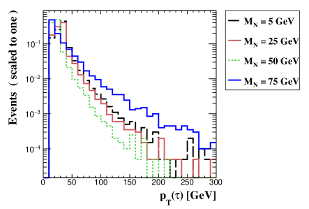
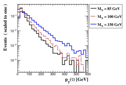
Figure 8: The transverse momentum $p_{T}(\tau)$ distribution of the $\tau$ lepton in the process $pp\rightarrow W^{\pm(\ast)}\rightarrow\tau^{\pm}N+X$ at $\sqrt{s}=14$ TeV for the same benchmark points as Fig. 7.

Based on the fact that the constraints on the mixing between $\nu_{\tau}$ and HNLs are relatively weaker than those of $\nu_{e}$ and $\nu_{\mu}$ in various HNL mass ranges, we study the channel $pp\rightarrow W^{\pm(\ast)}+X\rightarrow\tau^{\pm}N+X$ at the LHC 14 TeV to search for HNLs in this work. We first set $U^{2}_{eN}=U^{2}_{\mu N}=0$ and only focus on the $U^{2}_{\tau N}$ dependence in the above production channel. The $W$ boson propagator can be either on-shell or off-shell depending on the mass of HNLs. We apply the Heavy Neutrino model file Degrande:2016aje from the model database of FeynRules Alloul:2013bka and use Madgraph5 aMC@NLO Alwall:2014hca ; Frederix:2018nkq to simulate this production channel at tree level and include the emission of up to two additional partons. The $p_{T}(N)$ and $p_{T}(\tau)$ distributions for some benchmark points with $M_{N}<m_{W}$ ($M_{N}>m_{W}$) at parton level are shown in the left (right) panel of Figs. 7 and 8, respectively. Because of the mass thresholds of the $W$ boson and HNLs, the $p_{T}(N)$ and $p_{T}(\tau)$ are relatively soft for $M_{N}<m_{W}$, especially for the case of $M_{N}=75$ GeV. To identify and detect these soft final states are the main issue of this study. On the other hand, a detail study for the situation of $M_{N}\sim m_{W}$ is needed, and we leave this part in future.

The decay length $L_{N}$ of the HNLs can be simply estimated by $L_{N}=\gamma c\tau_{N}$ where $\tau_{N}=1/\Gamma_{N}$ and the Lorentz boost factor $\gamma$ can be approximated as $p_{T}(N)/M_{N}$. We expect that HNL is not very boosted in this production channel except for $M_{N}=5$ GeV in Fig. 7. Combined with the information from Figs. 2 and 3, there is still large allowed parameter space for prompt decays of HNLs in this production channel. Therefore, we focus on the case with prompt decays of HNLs first and leave the displaced vertex of HNLs aside in this paper.

IV.2 Signature of the signals and possible SM backgrounds

We first divide the signal region to two parts: (1) on-shell $W$ boson production region and (2) off-shell $W$ boson production region. Different analysis strategies will be applied to each signal and SM backgrounds in these two regions. We focus on those final states with two $\tau$ leptons and one additional charged lepton in this work, and will explore the signature of two same-sign $\tau$ leptons with two jets as Ref. Keung:1983uu ; Das:2017gke ; Das:2018usr in the future. As we known, the $\tau^{\pm}\tau^{\pm}jj$ search channel would suffer from the severe QCD backgrounds such that signal events may be easily submerged. Conversely, the signature of two $\tau$ leptons with one additional charged lepton can effectively reduce those huge QCD backgrounds, but we need to carefully exploit kinematic properties of the final states to discriminate between the signal and SM backgrounds.

Consider the following signal process

$$pp\rightarrow W^{\pm(\ast)}\rightarrow\tau^{\pm}N \rightarrow\tau^{\pm}\tau^{\pm}l^{\mp}_{\alpha}\overline{\nu_{\alpha}}(\nu_{\alpha})$$ (2)

$$\hookrightarrow\tau^{\pm}\tau^{\mp}l^{\pm}_{\alpha}\nu_{\alpha}(\overline{\nu_{\alpha}})$$

where $\alpha=e,\mu,\tau$. We can further classify the final states in the following three categories: (1) Two same-sign $\tau$s, $e/\mu$ and $mET$ ($\tau^{\pm}\tau^{\pm}e^{\mp}(\mu^{\mp})\overline{\nu_{e,\mu}}(\nu_{e,\mu})$), (2) Two opposite-sign $\tau$s, $e/\mu$ and $mET$ ($\tau^{+}\tau^{-}e^{\pm}(\mu^{\pm})\nu_{e,\mu}(\overline{\nu_{e,\mu}}$) and (3) Three $\tau$s and $mET$ ($\tau^{\pm}\tau^{\pm}\tau^{\mp}\overline{\nu_{\tau}}(\nu_{\tau})$). We will ignore the analysis of three $\tau$s and $mET$ final state, as we cannot distinguish the Majorana or Dirac nature of the HNL via the three $\tau$ leptons and $mET$ final state, in contrast to the first two categories.

As shown before, there are still some possibilities to search for displaced $\tau$ leptons events from the low $M_{N}$ region with small mixing angles. This kind of signature has been studied in Ref. Cottin:2018nms . Therefore, we mainly focus on the prompt $\tau$s in this work. On the other hand, $\tau$ leptons have both hadronic and leptonic decay modes. We choose hadronic $\tau$ lepton decays for all $\tau$ leptons in our study with the following two main reasons. First, hadronic $\tau$ lepton decays account for approximately $65\%$ of all possible $\tau$ lepton decay modes. Therefore, we can save more $\tau$ lepton decay events from hadronic decay modes than leptonic decay modes. Second, leptonic $\tau$ lepton decays can mimic the signals of only $e$’s and $\mu$’s in the final state which cannot be distinguished at the LHC.

There are some irreducible and reducible SM backgrounds for the above three categories of signatures. We first consider the signal signature with two same-sign $\tau$s, $e/\mu$ and $mET$, the backgrounds of which include

1. Irreducible SM backgrounds:
   $W^{\pm}W^{\pm}W^{\mp}$.

2. Reducible SM backgrounds:
   (1) EW processes : $W^{+}W^{-}Z/H/\gamma^{\ast}$.
   (2) $t\overline{t}$ associated processes: $t\overline{t}W^{\pm}/Z/H/\gamma^{\ast}$ and $t\overline{t}+nj$ $(n=0\mathchar 45\relax 2)$.
   (3) QCD multijets.

Then we consider the signal signature with two opposite-sign $\tau$s, $e/\mu$ and $mET$, the backgrounds of which include

1. Irreducible SM backgrounds:
   $W^{\pm}Z/H/\gamma^{\ast}$, and $W^{\pm}W^{\pm}W^{\mp}$.

2. Reducible SM backgrounds:
   (1) EW processes : $ZZ/H/\gamma^{\ast}$ and $W^{+}W^{-}Z/H/\gamma^{\ast}$.
   (2) $t\overline{t}$ associated processes: $t\overline{t}W^{\pm}/Z/H/\gamma^{\ast}$ and $t\overline{t}+nj$ $(n=0\mathchar 45\relax 2)$.
   (3) $\tau^{+}\tau^{-}+nj$ $(n=0\mathchar 45\relax 2)$.
   (4) QCD multijets.

Finally, the sources of SM backgrounds for the signal signature with three prompt $\tau$s and $mET$ are similar to those of two opposite-sign $\tau$s, $e/\mu$ and $mET$. We will not repeatedly list them again.

IV.3 Simulations and event selections

We use Madgraph5 aMC@NLO Alwall:2014hca ; Frederix:2018nkq to calculate the signal and background processes at leading order (LO) and generate MC events, perform parton showering and hadronization by Pythia8 Sjostrand:2007gs , and employ the detection simulations by Delphes3 deFavereau:2013fsa with the ATLAS template. The NNPDF2.3LO PDF set was used and ME-PS matching with MLM prescription Mangano:2006rw ; Alwall:2007fs was applied for all the signal and major SM backgrounds. We include the emission of up to two additional partons for the signals with a matching scale set to be $30$ GeV for $M_{N}\lesssim 120$ GeV and about one quarter of the $M_{N}$ for $M_{N}>120$ GeV. On the other hand, the matching scales for $t\overline{t}+nj$ and $\tau^{+}\tau^{-}+nj$ $(n=0\mathchar 45\relax 2)$ are set to be $20$ GeV and $30$ GeV, respectively. All jets are reconstructed using the the anti-$k_{T}$ algorithm Cacciari:2008gp in FastJets Cacciari:2011ma with a radius parameter of $R=0.6$. The procedures of hadronic tau lepton decay and reconstruction are as follows. We first set tau leptons to automatically decay through Pythia8, and use the ATLAS template in Delphes3 for the tau tagging algorithm according to the efficiencies shown in Ref. ATLAS:2019uhp to reconstruct hadronic tau lepton decay using the visible final states. Notice the tau lepton cannot be fully reconstructed because the part from neutrino becomes missing energy and is ignored from the hadronic tau reconstruction. Furthermore, the electron, muon efficiencies in Delphes3 are modified to include the low $P_{T}$ regions inspired from the Ref. Aad:2019qnd . In order to study the Majorana nature of HNLs at the LHC, we classify our simulations and event selections in (1) two same-sign $\tau$s, $e/\mu$ and $mET$ and (2) two opposite-sign $\tau$s, $\mu$ and $mET$.

IV.3.1 Two same-sign $\tau$s, $e/\mu$ and $mET$

In this scenario, we require two same-sign $\tau$ leptons with an additional $e/\mu$ in the final state with the following cut flow.

1. For $M_{N}<m_{W}$, we specifically take two soft same-sign $\tau$ leptons and an extra soft $e/\mu$ as the selection of signals in our events with the following conditions,

   $$N(\tau^{\pm},l^{\mp})\geqslant 2,1,\quad 5<P^{l}_{T}<40\;{\rm GeV},\quad|\eta^{l}|<2.5,\quad 20<P^{\tau_{1}(\tau_{2})}_{T}<50(40)\;{\rm GeV},\quad|\eta^{\tau}|<2.5\,,$$ (3)

   where $l=e,\mu$. Since $\tau$ leptons and $e/\mu$ are relatively soft in this case compared with SM backgrounds, we reject those high $P_{T}$ regions to reduce background contributions inspired from the Ref. Florez:2016lwi ; Aboubrahim:2017aen ; Sirunyan:2018iwl ; Sirunyan:2019mlu ; Aad:2019qnd . We follow Ref. ATLAS:2019uhp with $p^{min}_{T}>10$ GeV for jet-seeding of visible hadronic tau to start with and only visible hadronic tau candidates with $p^{min}_{T}>20$ GeV are used. However, we think it is still worthwhile to tell the readers about the situation with $p^{min}_{T}>15$ GeV as in Ref. Florez:2016lwi ; Aboubrahim:2017aen , so we place the cut flow tables for this case into Appendix B. On the other hand, for $M_{N}>m_{W}$, we only choose the following conditions for them:

   $$N(\tau^{\pm},l^{\mp})\geqslant 2,1,\quad P^{l}_{T}>10\;{\rm GeV},\quad|\eta^{l}|<2.5,\quad P^{\tau}_{T}>20\;{\rm GeV},\quad|\eta^{\tau}|<2.5\,,$$ (4)

   where $l=e,\mu$. Besides, the two same-sign $\tau$ candidates must be angularly separated enough by requiring $\Delta R_{\tau^{\pm}\tau^{\pm}}>0.6$ in order to avoid overlapping. Other isolation criteria among $e,\mu,\tau$ and jets are the same as the default settings of Delphes3.

2. In order to reduce the $\tau$ lepton pair from the Drell-Yan process, we veto any opposite-sign $\tau$ lepton for both the signal and backgrounds with

   $$N(\tau^{\mp})=0\quad{\rm with}\quad P^{\tau}_{T}>20\;{\rm GeV},\quad|\eta^{\tau}|<2.5\,.$$ (5)

3. To suppress the contributions from backgrounds of $t\overline{t}$ associated processes, we reject the high missing transverse momentum $P^{miss}_{T}$ events by requiring

   $$P^{miss}_{T}<40\,(M_{N}/2)\;{\rm GeV}\,,$$ (6)

   for $M_{N}<m_{W}$ ($M_{N}>m_{W}$).

4. To further reduce the contributions from backgrounds of $t\overline{t}$ associated processes, we apply the $b$-veto for both the signal and backgrounds with

   $$N(b)=0\quad{\rm with}\quad P^{b}_{T}>20\;{\rm GeV},\quad|\eta^{b}|<2.5\,.$$ (7)

   Moreover, for $M_{N}>m_{W}$, we further reduce background contributions by requiring the inclusive scalar sum of jet $E_{T}$, $H_{T}$ Pascoli:2018heg ; Liu:2019ayx , to satisfy

   $$H_{T}<200\;{\rm GeV}.$$ (8)

   The inclusive $H_{T}$ distributions for both signals and backgrounds are shown in Appendix B.

5. We require the minimum invariant mass for one of $\tau$ leptons and an extra $e/\mu$ to satisfy

   $$M_{\tau^{\pm}\ell_{1}^{\mp}}<M_{N}\,.$$ (9)

   This $\tau$ lepton is most likely to be the second energetic one for small $M_{N}$, but it becomes hard to be distinguished as $M_{N}$ increases. Here we use the transverse mass distribution for $MT_{\tau^{\pm}\ell_{1}^{\mp}P_{T}^{miss}}$ to find the correct $\tau$ lepton from the HNL decay. We plot both $MT_{\tau_{1}^{\pm}\ell_{1}^{\mp}P_{T}^{miss}}$ and $MT_{\tau_{2}^{\pm}\ell_{1}^{\mp}P_{T}^{miss}}$ distributions, and choose the one that closely indicates the mass of the HNL. The same $\tau$ lepton is used to form the invariant mass $M_{\tau^{\pm}\ell_{1}^{\mp}}$.

6. Finally, if $M_{N}<m_{W}$, the invariant mass of two same-sign $\tau$ leptons and an extra $e/\mu$ system is required to have

   $$M_{\tau_{1}^{\pm}\tau_{2}^{\pm}\ell_{1}^{\mp}}<m_{W}\,.$$ (10)

IV.3.2 Two opposite-sign $\tau$s, $\mu$ and $mET$

In this scenario, we require two opposite-sign $\tau$ leptons and an extra $\mu$ in the final state with the following cut flow.

1. For $M_{N}<m_{W}$, we specifically take two soft opposite-sign $\tau$ leptons and an extra soft $\mu$ as the selection of signals in our events with the following conditions,

   $$N(\tau,\mu)\geqslant 2,1,\quad 5<P^{\mu}_{T}<40\;{\rm GeV},\quad|\eta^{\mu}|<2.5,\quad 20<P^{\tau_{1}(\tau_{2})}_{T}<50(40)\;{\rm GeV},\quad|\eta^{\tau}|<2.5\,,$$ (11)

   On the other hand, for $M_{N}>m_{W}$, we choose instead the following conditions for them:

   $$N(\tau,\mu)\geqslant 2,1,\quad P^{\mu}_{T}>15\;{\rm GeV},\quad|\eta^{\mu}|<2.5,\quad P^{\tau}_{T}>20\;{\rm GeV},\quad|\eta^{\tau}|<2.5\,,$$ (12)

   Compared with Eq. (4), we require a stronger $P^{\mu}_{T}$ cut to further suppress soft radiation muons from $\tau\tau+nj$ and $t\bar{t}+nj$ processes. Again, $\Delta R_{\tau^{+}\tau^{-}}>0.6$ and other isolation criteria are set to avoid overlaps.

2. In order to reduce SM backgrounds with more than three $\tau$ leptons, we veto any same-sign $\tau$ lepton for both signal and backgrounds with the same conditions as Eq. (5).

3. To further reduce the contributions from backgrounds of $t\overline{t}$ associated processes, we apply the following cuts for both signal and backgrounds: high $P^{miss}_{T}$ rejection as Eq. (6), $b$-veto as Eq. (7). In addition, the cut $H_{T}<200\;{\rm GeV}$ is applied for $M_{N}>m_{W}$.

4. We require the minimum invariant mass for the $\tau$ leptons and an extra $\mu$ with opposite charges to satisfy Eq. (9). Compared with the case of same-sign $\tau$s, it becomes more precise to pick up the correct $\tau$ lepton from the HNL decay.

5. Finally, if $M_{N}<m_{W}$, the invariant mass of two opposite-sign $\tau$ leptons and an extra $\mu$ system is required to have

   $$M_{\tau^{+}\tau^{-}\mu}<m_{W}\,.$$ (13)

V Analysis and results at HL-LHC

V.1 Same-sign tau leptons plus a charged lepton

Two Same-Sign $\tau$s Selection Flow Table
Process	$\sigma$	Preselection	$P_{T}^{miss}<$ 40 GeV	b veto	Invariant Mass Selection
	(fb)	$A\epsilon$ (%)	$A\epsilon$ (%)	$A\epsilon$ (%)	$A\epsilon$ (%)
$M_{N}$ = 25 GeV	$2.851$	$9.834\times 10^{-1}$	$9.071\times 10^{-1}$	$8.860\times 10^{-1}$	$5.663\times 10^{-1}$
$W^{\pm}W^{\pm}W^{\mp}$	$1.828\times 10^{-1}$	$1.029$	$5.110\times 10^{-1}$	$5.030\times 10^{-1}$	$1.890\times 10^{-2}$
$W^{+}W^{-}Z/H/\gamma$	$1.065\times 10^{-1}$	$6.755\times 10^{-1}$	$3.047\times 10^{-1}$	$2.990\times 10^{-1}$	$1.440\times 10^{-2}$
$t\bar{t}+nj$	$2.357\times 10^{4}$	$6.415\times 10^{-2}$	$1.282\times 10^{-2}$	$1.864\times 10^{-3}$	$2.530\times 10^{-5}$
Process	$\sigma$	Preselection	$P_{T}^{miss}<$ 40 GeV	b veto	Invariant Mass Selection
	(fb)	$A\epsilon$ (%)	$A\epsilon$ (%)	$A\epsilon$ (%)	$A\epsilon$ (%)
$M_{N}$ = 50 GeV	$2.068$	$1.023$	$9.465\times 10^{-1}$	$9.255\times 10^{-1}$	$7.584\times 10^{-1}$
$W^{\pm}W^{\pm}W^{\mp}$	$1.828\times 10^{-1}$	$1.029$	$5.110\times 10^{-1}$	$5.030\times 10^{-1}$	$6.114\times 10^{-2}$
$W^{+}W^{-}Z/H/\gamma$	$1.065\times 10^{-1}$	$6.755\times 10^{-1}$	$3.047\times 10^{-1}$	$2.990\times 10^{-1}$	$4.565\times 10^{-2}$
$t\bar{t}+nj$	$2.357\times 10^{4}$	$6.415\times 10^{-2}$	$1.282\times 10^{-2}$	$1.864\times 10^{-3}$	$1.602\times 10^{-4}$
Process	$\sigma$	Preselection	$P_{T}^{miss}<$ 40 GeV	b veto	Invariant Mass Selection
	(fb)	$A\epsilon$ (%)	$A\epsilon$ (%)	$A\epsilon$ (%)	$A\epsilon$ (%)
$M_{N}$ = 75 GeV	$8.935\times 10^{-2}$	$7.486\times 10^{-1}$	$6.723\times 10^{-1}$	$6.512\times 10^{-1}$	$4.861\times 10^{-1}$
$W^{\pm}W^{\pm}W^{\mp}$	$1.828\times 10^{-1}$	$1.029$	$5.110\times 10^{-1}$	$5.030\times 10^{-1}$	$6.752\times 10^{-2}$
$W^{+}W^{-}Z/H/\gamma$	$1.065\times 10^{-1}$	$6.755\times 10^{-1}$	$3.047\times 10^{-1}$	$2.990\times 10^{-1}$	$4.955\times 10^{-2}$
$t\bar{t}+nj$	$2.357\times 10^{4}$	$6.415\times 10^{-2}$	$1.282\times 10^{-2}$	$1.864\times 10^{-3}$	$1.771\times 10^{-4}$

Table 1: The two same-sign $\tau$s selection flow table for HNLs with benchmark points of $M_{N}$ = $25$, $50$ and $75$ GeV with $U^{2}_{\tau N}=10^{-5}$. The preselection and invariant mass selection are written in the main text. The $A\epsilon$ for each selection is the total accepted efficiency in each step.

Two Same-Sign $\tau$s Selection Flow Table
Process	$\sigma$	Preselection	$P_{T}^{miss}<$ 85/2 GeV	b veto	$H_{T}<200$ GeV	Invariant Mass Selection
	(fb)	$A\epsilon$ (%)	$A\epsilon$ (%)	$A\epsilon$ (%)	$A\epsilon$ (%)	$A\epsilon$ (%)
$M_{N}$ = 85 GeV	$1.102\times 10^{-2}$	$2.488$	$1.525$	$1.484$	$1.321$	$1.124$
$W^{\pm}W^{\pm}W^{\mp}$	$1.713\times 10^{-1}$	$5.454$	$1.577$	$1.547$	$1.374$	$7.939\times 10^{-1}$
$W^{+}W^{-}Z/H/\gamma$	$5.824\times 10^{-2}$	8.036	1.937	1.892	1.395	$7.277\times 10^{-1}$
$t\bar{t}+nj$	$2.240\times 10^{4}$	$6.030\times 10^{-1}$	$1.218\times 10^{-1}$	$1.801\times 10^{-2}$	$4.654\times 10^{-3}$	$2.428\times 10^{-3}$
Process	$\sigma$	Preselection	$P_{T}^{miss}<$ 100/2 GeV	b veto	$H_{T}<200$ GeV	Invariant Mass Selection
	(fb)	$A\epsilon$ (%)	$A\epsilon$ (%)	$A\epsilon$ (%)	$A\epsilon$ (%)	$A\epsilon$ (%)
$M_{N}$ = 100 GeV	$8.461\times 10^{-3}$	$2.834$	$1.702$	$1.656$	$1.447$	$1.144$
$W^{\pm}W^{\pm}W^{\mp}$	$1.713\times 10^{-1}$	$5.455$	$2.019$	$1.980$	$1.751$	$1.170$
$W^{+}W^{-}Z/H/\gamma$	$5.824\times 10^{-2}$	8.036	2.496	2.438	1.779	$1.085$
$t\bar{t}+nj$	$2.240\times 10^{4}$	$6.031\times 10^{-1}$	$1.607\times 10^{-1}$	$2.383\times 10^{-2}$	$5.969\times 10^{-3}$	$4.199\times 10^{-3}$
Process	$\sigma$	Preselection	$P_{T}^{miss}<$ 125/2 GeV	b veto	$H_{T}<200$ GeV	Invariant Mass Selection
	(fb)	$A\epsilon$ (%)	$A\epsilon$ (%)	$A\epsilon$ (%)	$A\epsilon$ (%)	$A\epsilon$ (%)
$M_{N}$ = 125 GeV	$3.486\times 10^{-3}$	$8.227$	$5.871$	$5.708$	$4.683$	$4.087$
$W^{\pm}W^{\pm}W^{\mp}$	$1.713\times 10^{-1}$	$5.455$	$2.709$	$2.656$	$2.322$	$1.801$
$W^{+}W^{-}Z/H/\gamma$	$5.824\times 10^{-2}$	8.036	3.403	3.324	2.378	$1.7103$
$t\bar{t}+nj$	$2.240\times 10^{4}$	$6.031\times 10^{-1}$	$2.280\times 10^{-1}$	$3.420\times 10^{-2}$	$8.044\times 10^{-3}$	$6.526\times 10^{-3}$
Process	$\sigma$	Preselection	$P_{T}^{miss}<$ 150/2 GeV	b veto	$H_{T}<200$ GeV	Invariant Mass Selection
	(fb)	$A\epsilon$ (%)	$A\epsilon$ (%)	$A\epsilon$ (%)	$A\epsilon$ (%)	$A\epsilon$ (%)
$M_{N}$ = 150 GeV	$1.758\times 10^{-3}$	$1.201\times 10^{1}$	$8.953$	$8.703$	$6.637$	$6.047$
$W^{\pm}W^{\pm}W^{\mp}$	$1.713\times 10^{-1}$	$5.455$	$3.297$	$3.231$	$2.788$	$2.340$
$W^{+}W^{-}Z/H/\gamma$	$5.824\times 10^{-2}$	8.036	4.200	4.099	2.864	$2.264$
$t\bar{t}+nj$	$2.240\times 10^{4}$	$6.031\times 10^{-1}$	$2.951\times 10^{-1}$	$4.361\times 10^{-2}$	$9.966\times 10^{-3}$	$8.853\times 10^{-3}$

Table 2: The same as Table 1, but for HNLs with benchmark points of $M_{N}$ = $85$, $100$, $125$ and $150$ GeV with $U^{2}_{\tau N}=10^{-5}$.

In this section, we display our results based on the simulation and analysis strategies in the previous section. First, we explain our results for the channel of two same-sign $\tau$s, $e/\mu$ and $mET$. The cut flow tables for $M_{N}<m_{W}$ ($M_{N}=25,50,75$ GeV) and $M_{N}>m_{W}$ ($M_{N}=85,100,125,150$ GeV) are shown in the Table 1 and Table 2, respectively. Here we set $U^{2}_{\tau N}=10^{-5}$ for all benchmark points. We list three major SM backgrounds in these two tables: $W^{\pm}W^{\pm}W^{\mp}$, $W^{+}W^{-}Z/H/\gamma$ and $t\bar{t}+nj$. The $t\bar{t}+nj$ is the dominant one among them before applying the selection cuts. On the other hand, the notation of Preselection includes Eqs. (3), (4) and (5) and Invariant Mass Selection includes Eqs. (9) and (10) (when $M_{N}<m_{W}$).

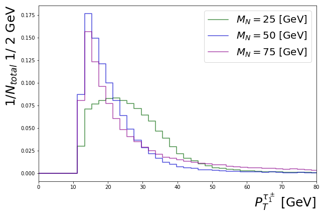
(a) The $p_{T}$ distribution for leading $\tau^{\pm}$

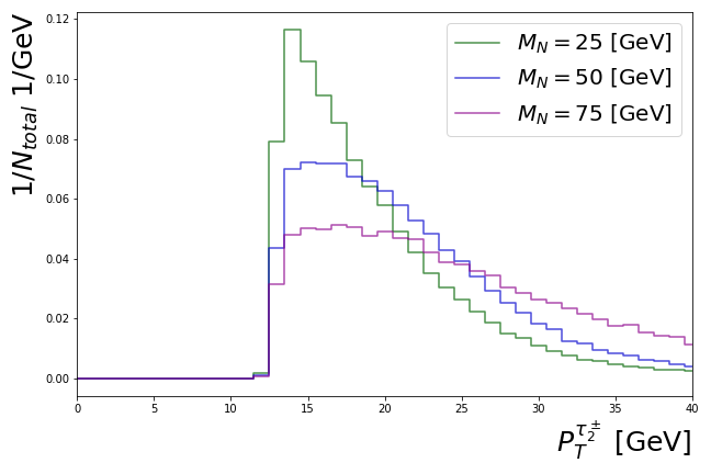
(b) The $p_{T}$ distribution for subleading $\tau^{\pm}$

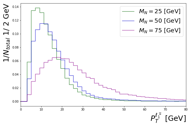
(c) The $p_{T}$ distribution for leading $\ell^{\mp}$

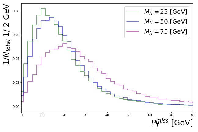
(d) The $p_{T}$ distribution for missing energy

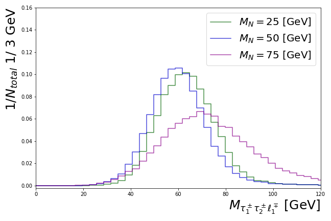
(e) The distribution for $M_{\tau_{1}^{\pm}\tau_{2}^{\pm}\ell_{1}^{\mp}}$

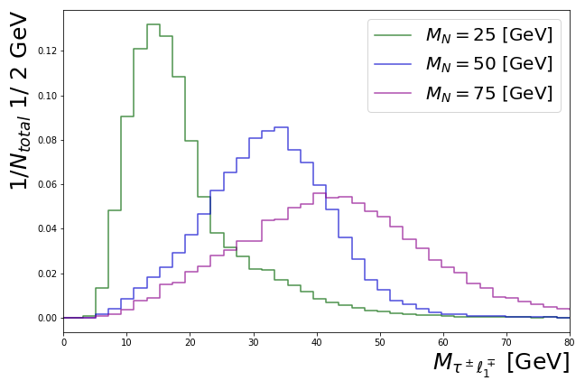
(f) The distribution for $M_{\tau^{\pm}\ell_{1}^{\mp}}$

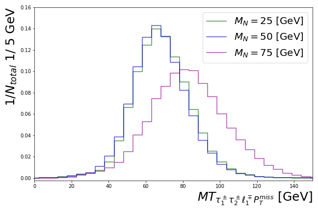
(g) The distribution for $MT_{\tau_{1}^{\pm}\tau_{2}^{\pm}\ell_{1}^{\mp}P_{T}^{miss}}$

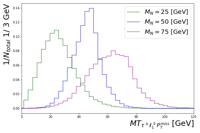
(h) The distribution for $MT_{\tau^{\pm}\ell_{1}^{\mp}P_{T}^{miss}}$

Figure 9: Two Same-Sign $\tau$s: Various kinematical distributions for the signal with the benchmark points of $M_{N}$ = $25$, $50$ and $75$ GeV. Notice the distributions in (e), (f), (g) and (h) passed the preselection criteria.

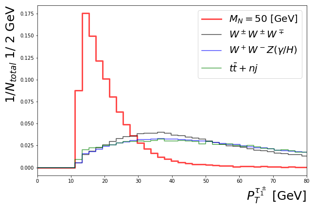
(a) The $p_{T}$ distribution for leading $\tau^{\pm}$

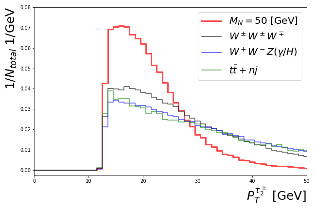
(b) The $p_{T}$ distribution for subleading $\tau^{\pm}$

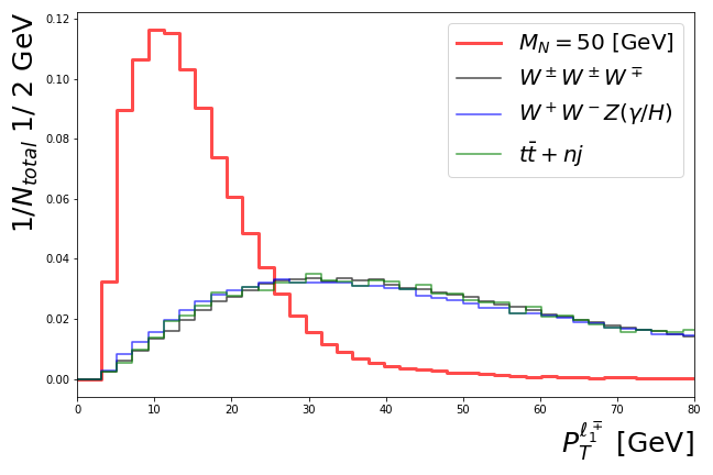
(c) The $p_{T}$ distribution for leading $\ell^{\mp}$

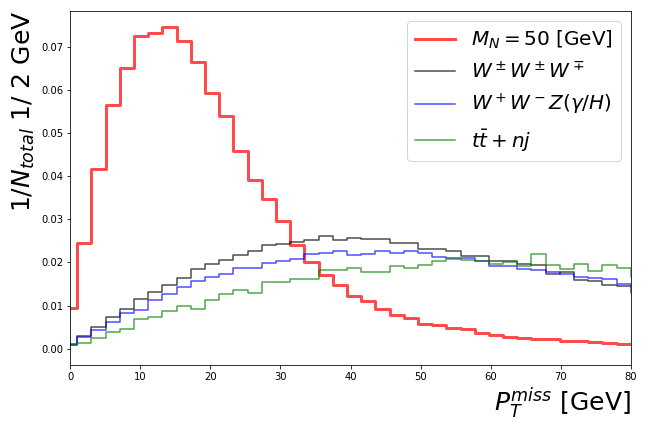
(d) The $p_{T}$ distribution for missing energy

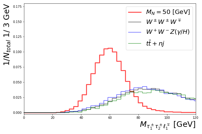
(e) The distribution for $M_{\tau_{1}^{\pm}\tau_{2}^{\pm}\ell_{1}^{\mp}}$

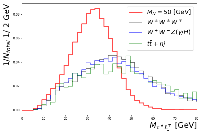
(f) The distribution for $M_{\tau^{\pm}\ell_{1}^{\mp}}$

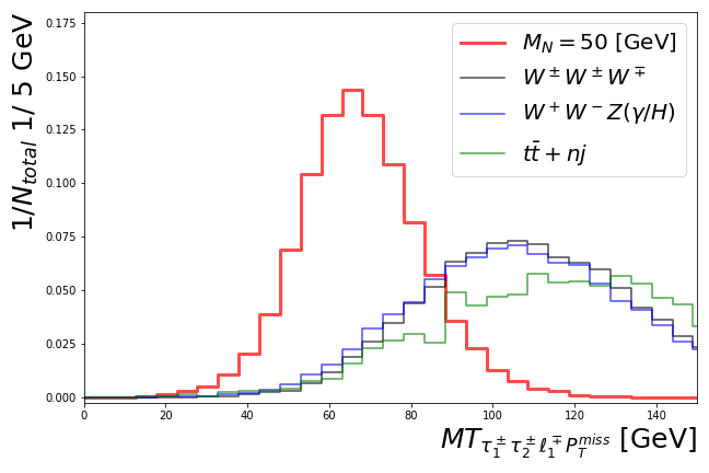
(g) The distribution for $MT_{\tau_{1}^{\pm}\tau_{2}^{\pm}\ell_{1}^{\mp}P_{T}^{miss}}$

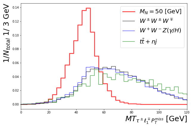
(h) The distribution for $MT_{\tau^{\pm}\ell_{1}^{\mp}P_{T}^{miss}}$

Figure 10: The same as Fig. 9, but for the signal with the benchmark point of $M_{N}=50$ GeV and major SM backgrounds.

For $M_{N}<m_{W}$, after passing all selection cuts, we can find the signal efficiencies around $0.49\mathchar 45\relax 0.57\%$, the efficiencies of $W^{\pm}W^{\pm}W^{\mp}$ and $W^{+}W^{-}Z/H/\gamma$ are less than $6.8\times 10^{-2}\%$ and $5.0\times 10^{-2}\%$, and that of $t\bar{t}+nj$ is even smaller, less than $2.5\times 10^{-5}\%$. Some kinematical distributions for the signal with $M_{N}=25$, $50$ and 75 GeV are shown in Fig. 9. Notice that the distributions in (e), (f), (g) and (h) pass the preselection criteria. All $\tau_{1}$, $\tau_{2}$ and $\ell_{1}$ are relatively soft as shown in (a), (b) and (c) on Fig 9. In order to pick out these soft objects, we focus on low $P_{T}$ regions as in Eq. (3). Similar to the soft charged leptons, the $P^{miss}_{T}$ is also soft as shown in (d) in Fig 9, so we further reject the high $P^{miss}_{T}$ regions as in Eq. (6). Finally, Eqs. (9) and (10) can help us to select the major parts of the signal as shown in (e) and (f) in Fig. 9. On the other hand, the transverse mass distribution for $M_{T}(P^{\tau^{\pm}_{1}}_{T},P^{\tau^{\pm}_{2}}_{T},P^{\ell^{\mp}_{1}}_{T},P^{miss}_{T})$ and $M_{T}(P^{\tau^{\pm}}_{T},P^{\ell^{\mp}_{1}}_{T},P^{miss}_{T})$ in (g) and (h) in Fig. 9 clearly show the resonance structure of both $m_{W}$ and $M_{N}$, respectively. In Fig. 10, we also display these kinematical distributions for the signal $M_{N}=50$ GeV and three major SM backgrounds. We can clearly see that these analysis strategies for this scenario in the previous section can successfully distinguish most parts of the signal from the SM backgrounds.

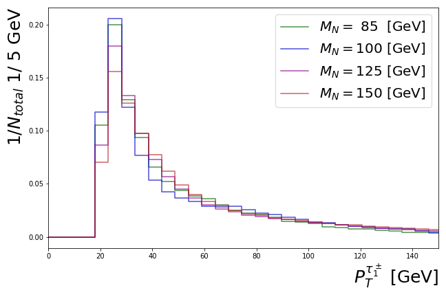
(a) The $p_{T}$ distribution for leading $\tau^{\pm}$

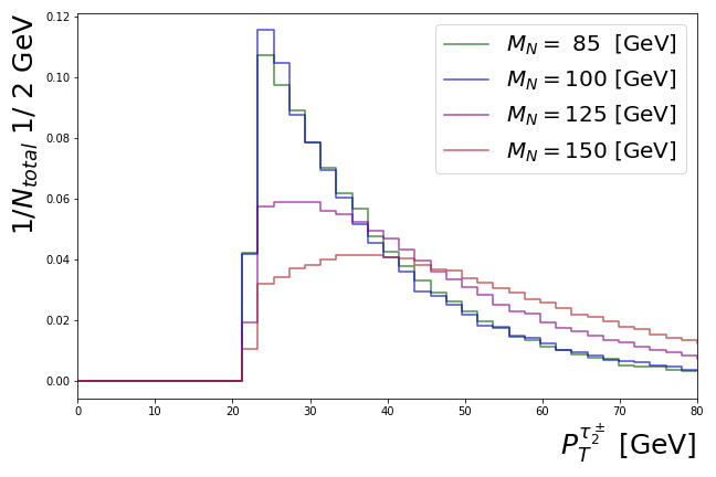
(b) The $p_{T}$ distribution for subleading $\tau^{\pm}$

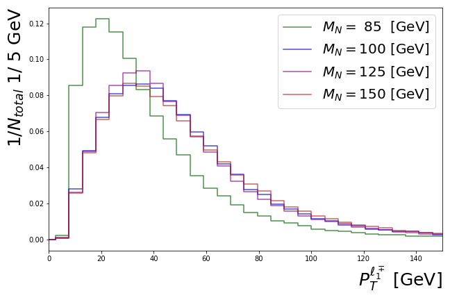
(c) The $p_{T}$ distribution for leading $\ell^{\mp}$

(d) The $p_{T}$ distribution for missing energy

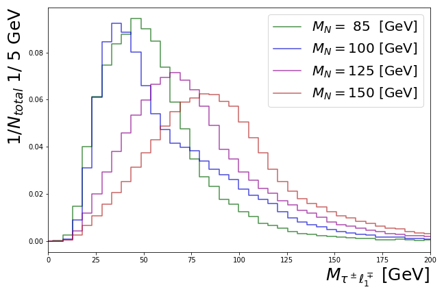
(e) The distribution for $M_{\tau^{\pm}\ell_{1}^{\mp}}$

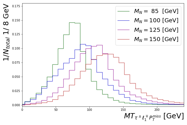
(f) The distribution for $MT_{\tau^{\pm}\ell_{1}^{\mp}P_{T}^{miss}}$

Figure 11: Two Same-Sign $\tau$s: various kinematical distributions for the signal with the benchmark points of $M_{N}=85$, $100$, $125$ and $150$ GeV. Notice the distributions in (e) and (f) passed the preselection criteria.

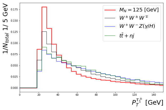
(a) The $p_{T}$ distribution for leading $\tau^{\pm}$

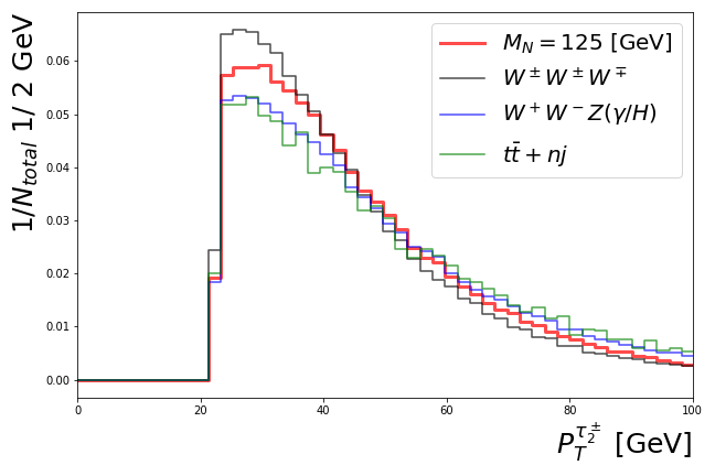
(b) The $p_{T}$ distribution for subleading $\tau^{\pm}$

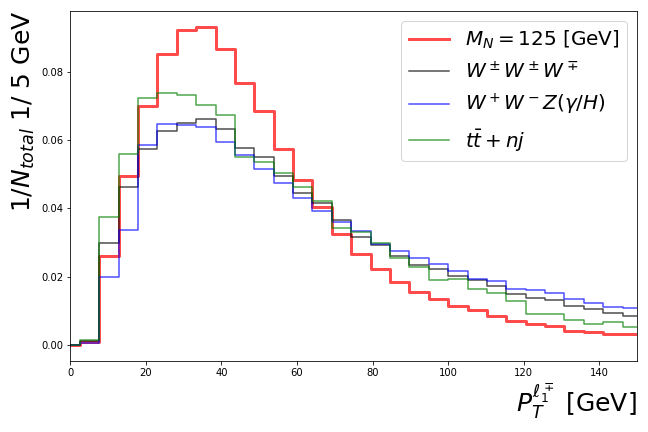
(c) The $p_{T}$ distribution for leading $\ell^{\mp}$

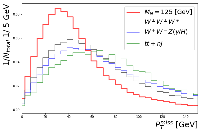
(d) The $p_{T}$ distribution for missing energy

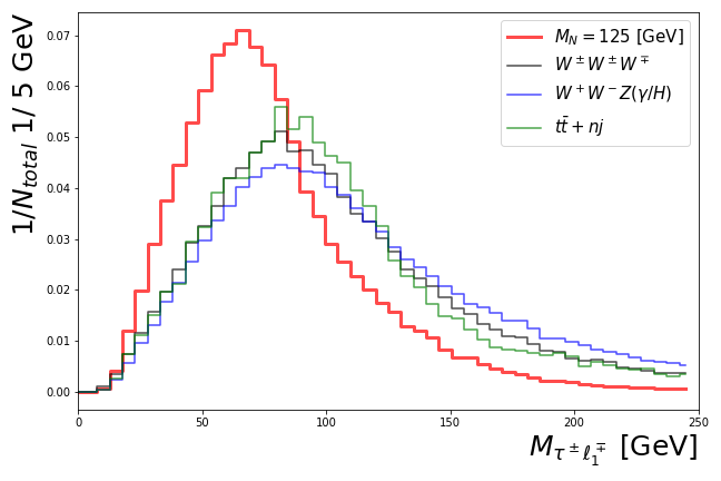
(e) The distribution for $M_{\tau^{\pm}\ell_{1}^{\mp}}$

(f) The distribution for $MT_{\tau^{\pm}\ell_{1}^{\mp}P_{T}^{miss}}$

Figure 12: The same as Fig. 11, but for the signal with the benchmark point of $M_{N}=125$ GeV and major SM backgrounds.

For $M_{N}>m_{W}$, after passing all selection cuts, we can find the signal efficiencies around $1.1\mathchar 45\relax 6.0\%$, the efficiencies of $W^{\pm}W^{\pm}W^{\mp}$ and $W^{+}W^{-}Z/H/\gamma$ are less than $2.3\%$, and the efficiencies of $t\bar{t}+nj$ is even smaller, less than $8.9\times 10^{-3}\%$. Some kinematical distributions for the signal with $M_{N}=85$, $100$, $125$ and $150$ GeV are shown in Fig. 11. Notice that the distributions in (e) and (f) pass the preselection criteria. In contrast to the case $M_{N}<m_{W}$, as shown in (a), (b) and (c) in Fig. 11, $\tau$ leptons and $e/\mu$ can have long tail $P_{T}$ distributions with the increase in the mass of HNLs. We can also find most of $P^{miss}_{T}$ distributions in this scenario are less than $M_{N}/2$ as shown in (d) in Fig. 11. For the benchmark points of $M_{N}>85$ GeV, $N$ decays into an on-shell $W$ boson and a relatively soft $\tau$ because of the mass threshold. Thus, the subleading $\tau$ lepton shows a soft $P_{T}$ spectrum especially for the low mass shown in panel (b) of Fig. 11. Both the invariant mass $M_{\tau^{\pm}\ell_{1}^{\mp}}$ (panel (e)) and the transverse mass (panel (f)) distributions clearly correlate with the mass of the HNL. In Fig. 12, we also display these kinematical distributions for the signal benchmark $M_{N}=125$ GeV and three major SM backgrounds. All the major backgrounds show relatively harder spectra in $P_{T}^{\ell_{1}^{\mp}}$, $P_{T}^{miss}$, $M_{\tau^{\pm}\ell_{1}^{\mp}}$, and $M_{T_{\tau^{\pm}\ell_{1}^{\mp}P_{T}^{miss}}}$. One can make use of these features to discriminate the signal from the backgrounds.

Two Opposite-Sign $\tau$s Selection Flow Table
Process	$\sigma$	Preselection	$P_{T}^{miss}<$ 40 GeV	b veto	Invariant Mass Selection
	(fb)	$A\epsilon$ (%)	$A\epsilon$ (%)	$A\epsilon$ (%)	$A\epsilon$ (%)
$M_{N}$ = 25 GeV	$2.291$	$8.487\times 10{-1}$	$7.629\times 10{-1}$	$7.478\times 10{-1}$	$6.132\times 10{-1}$
$W^{\pm}Z/H/\gamma$	$1.599\times 10^{2}$	$7.696\times 10^{-1}$	$5.737\times 10^{-1}$	$5.652\times 10^{-1}$	$1.700\times 10^{-2}$
$ZZ/\gamma$	$2.400\times 10^{1}$	$7.990\times 10^{-1}$	$7.066\times 10^{-1}$	$6.967\times 10^{-1}$	$3.970\times 10^{-2}$
$\tau\tau+nj$	$9.559\times 10^{5}$	$3.680\times 10^{-4}$	$3.476\times 10^{-4}$	$3.476\times 10^{-4}$	$0$
$t\bar{t}+nj$	$2.987\times 10^{4}$	$2.164\times 10^{-2}$	$4.353\times 10^{-3}$	$5.804\times 10^{-4}$	$5.128\times 10^{-5}$
Process	$\sigma$	Preselection	$P_{T}^{miss}<$ 40 GeV	b veto	Invariant Mass Selection
	(fb)	$A\epsilon$ (%)	$A\epsilon$ (%)	$A\epsilon$ (%)	$A\epsilon$ (%)
$M_{N}$ = 50 GeV	$2.052$	$6.320\times 10{-1}$	$5.581\times 10{-1}$	$5.450\times 10{-1}$	$4.791\times 10{-1}$
$W^{\pm}Z/H/\gamma$	$1.599\times 10^{2}$	$7.696\times 10^{-1}$	$5.737\times 10^{-1}$	$5.652\times 10^{-1}$	$5.430\times 10^{-2}$
$ZZ/\gamma$	$2.400\times 10^{1}$	$7.990\times 10^{-1}$	$7.066\times 10^{-1}$	$6.967\times 10^{-1}$	$9.740\times 10^{-2}$
$\tau\tau+nj$	$9.559\times 10^{5}$	$3.680\times 10^{-4}$	$3.476\times 10^{-4}$	$3.476\times 10^{-4}$	$6.134\times 10{-5}$
$t\bar{t}+nj$	$2.987\times 10^{4}$	$2.164\times 10^{-2}$	$4.353\times 10^{-3}$	$5.804\times 10^{-4}$	$1.878\times 10^{-4}$
Process	$\sigma$	Preselection	$P_{T}^{miss}<$ 40 GeV	b veto	Invariant Mass Selection
	(fb)	$A\epsilon$ (%)	$A\epsilon$ (%)	$A\epsilon$ (%)	$A\epsilon$ (%)
$M_{N}$ = 75 GeV	$9.104\times 10^{-2}$	$4.364\times 10^{-1}$	$3.429\times 10^{-1}$	$3.368\times 10^{-1}$	$1.619\times 10^{-1}$
$W^{\pm}Z/H/\gamma$	$1.599\times 10^{2}$	$7.696\times 10^{-1}$	$5.737\times 10^{-1}$	$5.652\times 10^{-1}$	$5.860\times 10^{-2}$
$ZZ/\gamma$	$2.400\times 10^{1}$	$7.990\times 10^{-1}$	$7.066\times 10^{-1}$	$6.967\times 10^{-1}$	$1.010\times 10^{-2}$
$\tau\tau+nj$	$9.559\times 10^{5}$	$3.680\times 10^{-4}$	$3.476\times 10^{-4}$	$3.476\times 10^{-4}$	$8.179\times 10{-5}$
$t\bar{t}+nj$	$2.987\times 10^{4}$	$2.164\times 10^{-2}$	$4.353\times 10^{-3}$	$5.804\times 10^{-4}$	$2.561\times 10^{-4}$

Table 3: The two opposite-sign $\tau$s selection flow table for HNLs with benchmark points of $M_{N}$ = 25, 50 and 75 GeV with $U^{2}_{\tau N}=10^{-5}$. The preselection and invariant mass selection are written in the main text. The $A\epsilon$ for each selection is the total accepted efficiency in each step.

Two Opposite-Sign $\tau$s Selection Flow Table
Process	$\sigma$	Preselection	$P_{T}^{miss}<$ 85/2 GeV	b veto	$H_{T}<200$ GeV	Invariant Mass Selection
	(fb)	$A\epsilon$ (%)	$A\epsilon$ (%)	$A\epsilon$ (%)	$A\epsilon$ (%)	$A\epsilon$ (%)
$M_{N}$ = 85 GeV	$1.101\times 10^{-2}$	$1.386$	$7.410\times 10^{-1}$	$7.236\times 10^{-1}$	$6.538\times 10^{-1}$	$6.471\times 10^{-1}$
$W^{\pm}Z/H/\gamma$	$1.031\times 10^{2}$	$4.402$	$2.004$	$1.971$	$1.874$	$1.078$
$ZZ/\gamma$	$2.082\times 10^{1}$	5.275	2.616	2.572	2.490	$1.339$
$\tau\tau+nj$	$9.561\times 10^{5}$	$2.024\times 10^{-4}$	$1.518\times 10^{-4}$	$1.417\times 10^{-4}$	$1.214\times 10^{-4}$	$1.012\times 10^{-4}$
$t\bar{t}+nj$	$2.864\times 10^{4}$	$2.712\times 10^{-1}$	$4.881\times 10^{-2}$	$7.395\times 10^{-3}$	$20118\times 10^{-3}$	$9.980\times 10^{-4}$
Process	$\sigma$	Preselection	$P_{T}^{miss}<$ 100/2 GeV	b veto	$H_{T}<200$ GeV	Invariant Mass Selection
	(fb)	$A\epsilon$ (%)	$A\epsilon$ (%)	$A\epsilon$ (%)	$A\epsilon$ (%)	$A\epsilon$ (%)
$M_{N}$ = 100 GeV	$8.745\times 10^{-3}$	$1.723$	$9.382\times 10^{-1}$	$9.144\times 10^{-1}$	$8.201\times 10^{-1}$	$8.140\times 10^{-1}$
$W^{\pm}Z/H/\gamma$	$1.031\times 10^{2}$	4.402	2.403	2.363	2.232	$1.516$
$ZZ/\gamma$	$2.082\times 10^{1}$	5.275	3.078	3.026	2.916	$1.938$
$\tau\tau+nj$	$9.561\times 10^{5}$	$2.024\times 10^{-4}$	$1.822\times 10^{-4}$	$1.720\times 10^{-4}$	$1.417\times 10^{-4}$	$1.012\times 10^{-4}$
$t\bar{t}+nj$	$2.864\times 10^{4}$	$2.712\times 10^{-1}$	$6.499\times 10^{-2}$	$9.595\times 10^{-3}$	$3.076\times 10^{-3}$	$2.159\times 10^{-3}$
Process	$\sigma$	Preselection	$P_{T}^{miss}<$ 125/2 GeV	b veto	$H_{T}<200$ GeV	Invariant Mass Selection
	(fb)	$A\epsilon$ (%)	$A\epsilon$ (%)	$A\epsilon$ (%)	$A\epsilon$ (%)	$A\epsilon$ (%)
$M_{N}$ = 125 GeV	$3.597\times 10^{-3}$	$4.683$	$3.186$	$3.101$	$2.609$	$2.605$
$W^{\pm}Z/H/\gamma$	$1.031\times 10^{2}$	$4.402$	$2.927$	$2.875$	$2.694$	$2.154$
$ZZ/\gamma$	$2.082\times 10^{1}$	5.275	3.694	3.630	3.472	$2.778$
$\tau\tau+nj$	$9.561\times 10^{5}$	$2.024\times 10^{-4}$	$1.923\times 10^{-4}$	$1.822\times 10^{-4}$	$1.518\times 10^{-4}$	$1.316\times 10^{-4}$
$t\bar{t}+nj$	$2.864\times 10^{4}$	$2.712\times 10^{-1}$	$9.252\times 10^{-2}$	$1.328\times 10^{-2}$	$4.196\times 10^{-3}$	$3.544\times 10^{-3}$
Process	$\sigma$	Preselection	$P_{T}^{miss}<$ 150/2 GeV	b veto	$H_{T}<200$ GeV	Invariant Mass Selection
	(fb)	$A\epsilon$ (%)	$A\epsilon$ (%)	$A\epsilon$ (%)	$A\epsilon$ (%)	$A\epsilon$ (%)
$M_{N}$ = 150 GeV	$1.800\times 10^{-3}$	$6.746$	$4.808$	$4.682$	$3.630$	$3.626$
$W^{\pm}Z/H/\gamma$	$1.031\times 10^{2}$	$4.402$	$3.314$	$3.254$	$3.020$	$2.631$
$ZZ/\gamma$	$2.082\times 10^{1}$	5.275	4.125	4.051	3.844	$3.378$
$\tau\tau+nj$	$9.561\times 10^{5}$	$2.024\times 10^{-4}$	$1.923\times 10^{-4}$	$1.822\times 10^{-4}$	$1.518\times 10^{-4}$	$1.518\times 10^{-4}$
$t\bar{t}+nj$	$2.864\times 10^{4}$	$2.712\times 10^{-1}$	$1.209\times 10^{-1}$	$1.719\times 10^{-2}$	$5.214\times 10^{-3}$	$4.643\times 10^{-3}$

Table 4: The same as Tab. 3, but for HNLs with benchmark points of $M_{N}$ = 85, 100, 125 and 150 GeV with $U^{2}_{\tau N}=10^{-5}$.

V.2 Opposite-sign tau leptons plus a muon

Now we turn to our results for the channel of two opposite-sign $\tau$s, $\mu$ and $mET$. The cut flow tables for $M_{N}<m_{W}$ ($M_{N}=25,50,75$ GeV) and $M_{N}>m_{W}$ ($M_{N}=85,100,125,150$ GeV) are shown in Tables 3 and 4, respectively. Again, we set $U^{2}_{\tau N}=10^{-5}$ for all benchmark points. We list four major SM backgrounds in these two tables: $W^{\pm}Z/H/\gamma$, $ZZ/\gamma$, $\tau\tau+nj$ and $t\bar{t}+nj$. The $\tau\tau+nj$ is the dominant one among them. The notation of Preselection includes Eqs. (11), (12) and (5) and Invariant Mass Selection includes Eqs. (9) and (13) (when $M_{N}<m_{W}$).

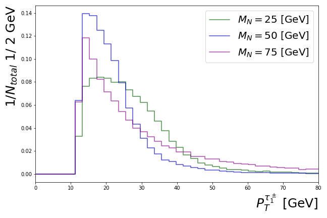
(a) The $p_{T}$ distribution for leading $\tau^{\pm}$

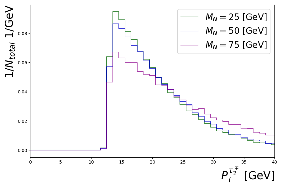
(b) The $p_{T}$ distribution for subleading $\tau^{\mp}$

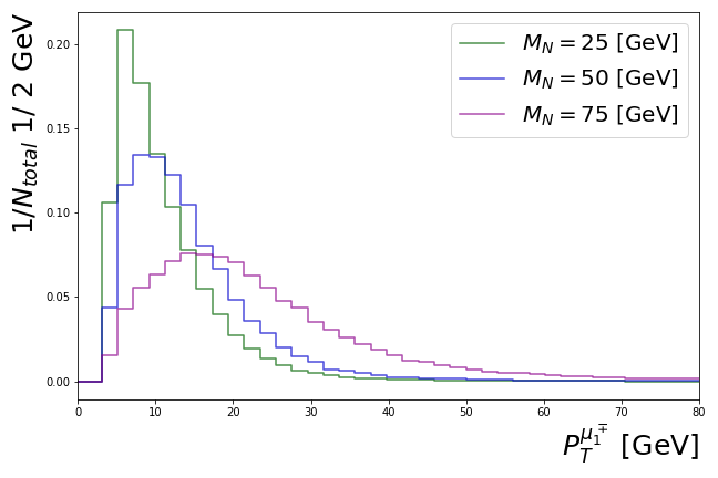
(c) The $p_{T}$ distribution for leading $\mu^{\mp}$

(d) The $p_{T}$ distribution for missing energy

(e) The distribution for $M_{\tau_{1}^{\mp}\tau_{2}^{\pm}\mu_{1}^{\mp}}$

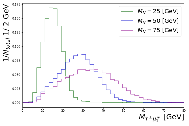
(f) The distribution for $M_{\tau^{\pm}\mu_{1}^{\mp}}$

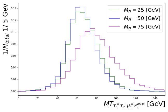
(g) The distribution for $MT_{\tau_{1}^{\mp}\tau_{2}^{\pm}\mu_{1}^{\mp}P_{T}^{miss}}$

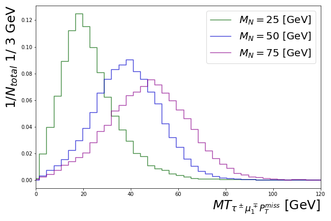
(h) The distribution for $MT_{\tau^{\pm}\mu_{1}^{\mp}P_{T}^{miss}}$

Figure 13: Two Opposite-Sign $\tau$s: various kinematical distributions for the signal with the benchmark points of $M_{N}=25$, $50$ and $75$ GeV. Notice the distributions in (e), (f), (g) and (h) passed the preselection criteria.

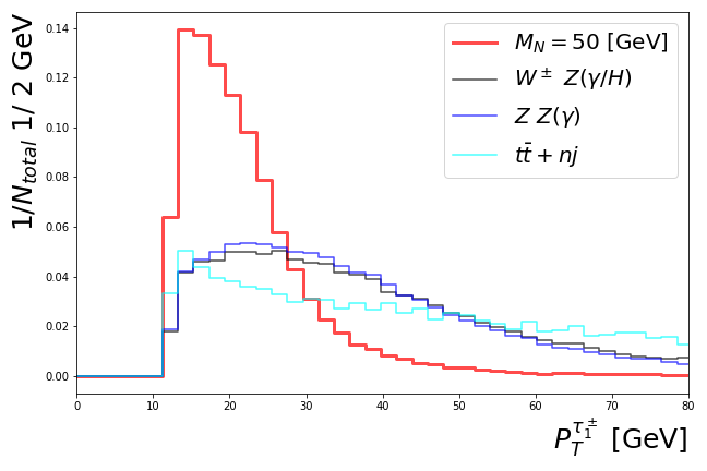
(a) The $p_{T}$ distribution for leading $\tau^{\pm}$

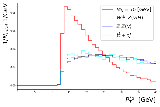
(b) The $p_{T}$ distribution for subleading $\tau^{\mp}$

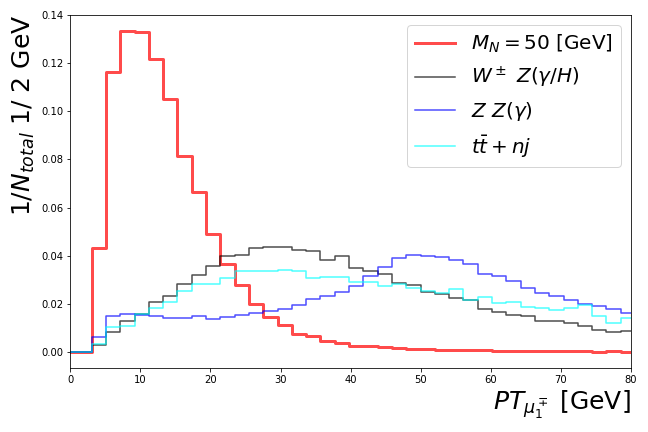
(c) The $p_{T}$ distribution for leading $\mu^{\mp}$

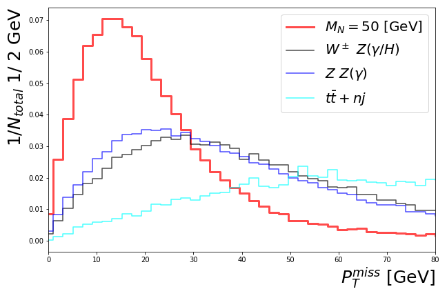
(d) The $p_{T}$ distribution for missing energy

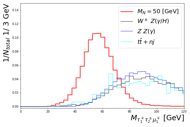
(e) The distribution for $M_{\tau_{1}^{\mp}\tau_{2}^{\pm}\mu_{1}^{\mp}}$

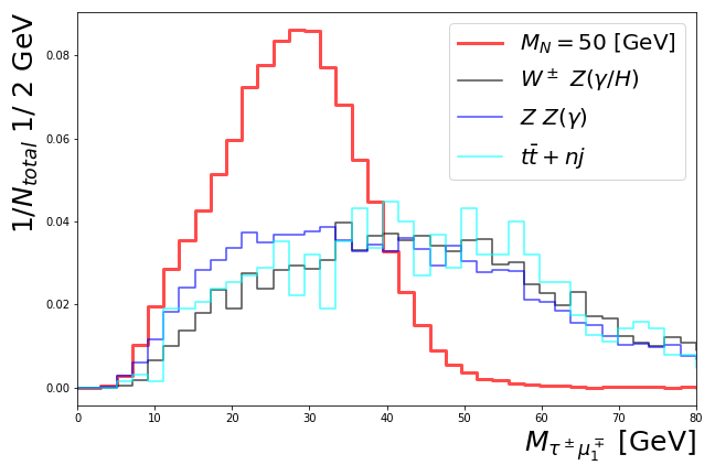
(f) The distribution for $M_{\tau^{\pm}\mu_{1}^{\mp}}$

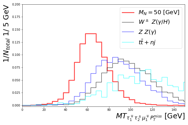
(g) The distribution for $MT_{\tau_{1}^{\mp}\tau_{2}^{\pm}\mu_{1}^{\mp}P_{T}^{miss}}$

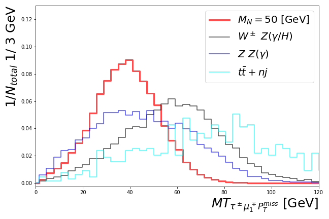
(h) The distribution for $MT_{\tau^{\pm}\mu_{1}^{\mp}P_{T}^{miss}}$

Figure 14: The same as Fig. 13, but for the signal with the benchmark point of $M_{N}=50$ GeV and major SM backgrounds.

For $M_{N}<m_{W}$, after passing all selection cuts, we can find the signal efficiencies around $0.16\mathchar 45\relax 0.61\%$, the efficiencies of $W^{\pm}Z/H/\gamma$ and $ZZ/\gamma$ are less than $5.9\times 10^{-2}\%$ and $9.7\times 10^{-2}\%$, and that of $\tau\tau+nj$ and $t\bar{t}+nj$ are even smaller, less than $8.2\times 10^{-5}\%$ and $5.1\times 10^{-5}\%$, respectively. Various kinematical distributions for the signal with $M_{N}=25$, $50$ and $75$ GeV are shown in Fig. 13. These distributions are similar to Fig. 9 except for panels (a), (b) and (c) in Fig. 13. This is due to the different helicity structures between $N\rightarrow\tau^{+}l^{-}_{\alpha}\overline{\nu_{\alpha}}$ and $N\rightarrow\tau^{-}l^{+}_{\alpha}\nu_{\alpha}$ that involve the $W$ propagator with only the left-handed interaction, and causing the variation of $P^{l}_{T}$ and $P^{\tau}_{T}$ distributions. In Fig 14, we also display these kinematical distributions for the signal $M_{N}=50$ GeV and three major SM backgrounds. We do not show kinematical distributions for $\tau\tau+nj$ process because only very few events can pass the preselection criteria. As we expected, these selection criteria can also successfully distinguish most parts of the signal from SM backgrounds.

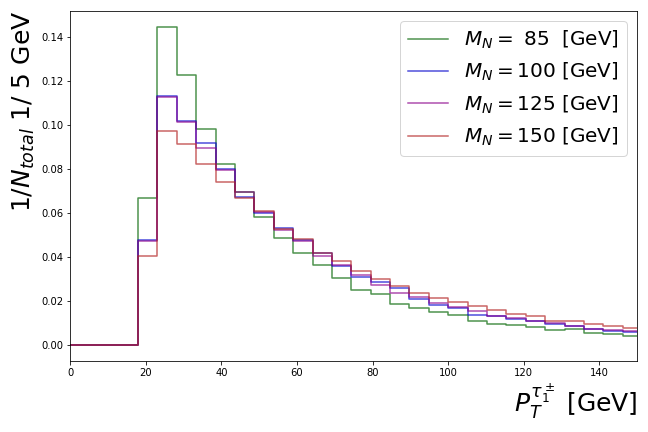
(a) The $p_{T}$ distribution for leading $\tau^{\pm}$

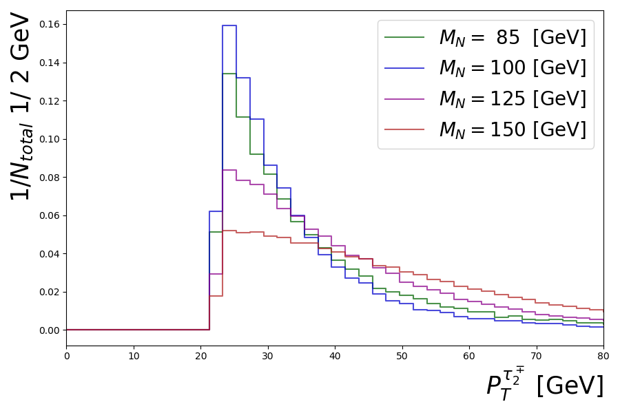
(b) The $p_{T}$ distribution for subleading $\tau^{\mp}$

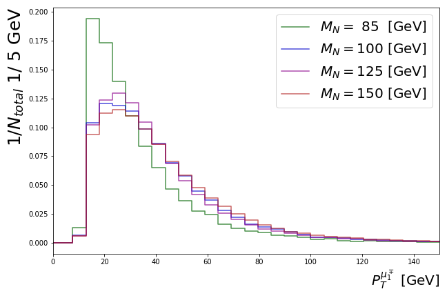
(c) The $p_{T}$ distribution for leading $\mu^{\mp}$

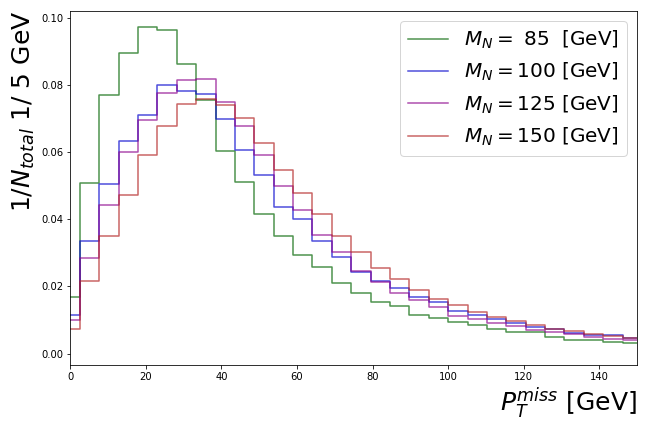
(d) The $p_{T}$ distribution for missing energy

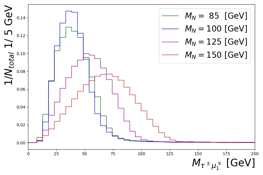
(e) The distribution for $M_{\tau^{\pm}\mu_{1}^{\mp}}$

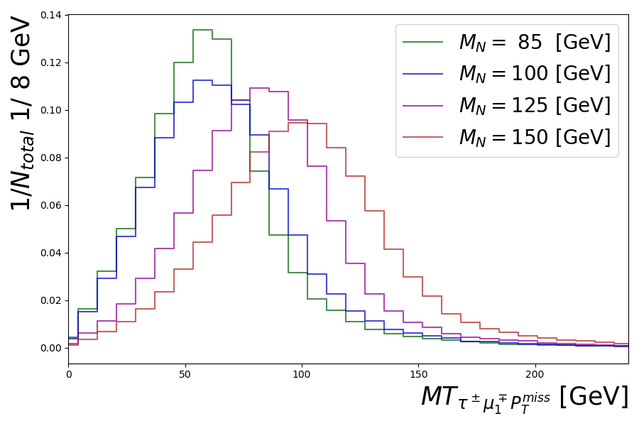
(f) The distribution for $MT_{\tau^{\pm}\mu_{1}^{\mp}P_{T}^{miss}}$

Figure 15: Two Opposite-Sign $\tau$s: various kinematical distributions for the signal with the benchmark points of $M_{N}=85$, $100$, $125$ and $150$ GeV. Notice the distributions in (e) and (f) passed the preselection criteria.

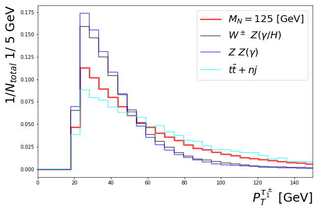
(a) The $p_{T}$ distribution for leading $\tau^{\pm}$

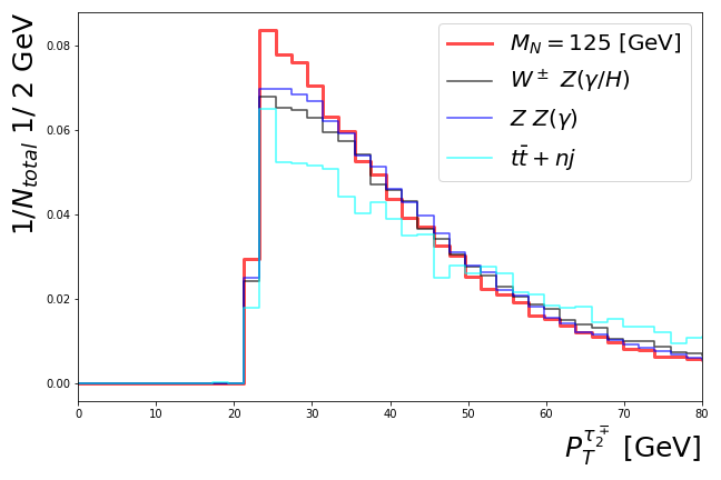
(b) The $p_{T}$ distribution for subleading $\tau^{\mp}$

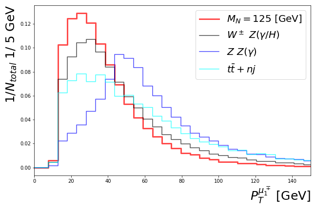
(c) The $p_{T}$ distribution for leading $\mu^{\mp}$

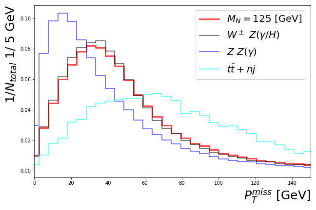
(d) The $p_{T}$ distribution for missing energy

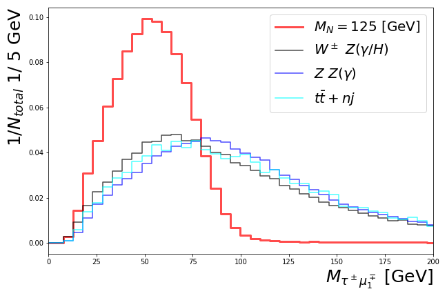
(e) The distribution for $M_{\tau^{\pm}\mu_{1}^{\mp}}$

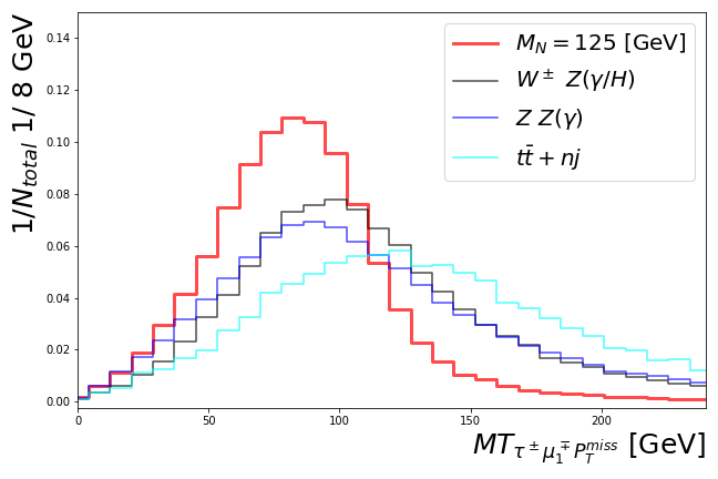
(f) The distribution for $MT_{\tau^{\pm}\mu_{1}^{\mp}P_{T}^{miss}}$

Figure 16: The same as Fig. 15 but for the signal with the benchmark point of $M_{N}=125$ GeV and major SM backgrounds.

For $M_{N}>m_{W}$, after imposing all selection cuts, we can find the signal efficiencies around $0.65\mathchar 45\relax 3.63\%$, the efficiencies of $W^{\pm}Z/H/\gamma$ and $ZZ/\gamma$ are less than $2.63\%$ and $3.38\%$, and those of $\tau\tau+nj$ and $t\bar{t}+nj$ are even smaller, less than $1.52\times 10^{-4}\%$ and $4.64\times 10^{-3}\%$, respectively. Various kinematical distributions for the signal with $M_{N}=85$, $100$, $125$ and $150$ GeV are shown in Fig. 15. Again, these distributions are similar to Fig. 11. In Fig. 16, we also display these kinematical distributions for the signal $M_{N}=125$ GeV and three major SM backgrounds. Again, kinematical distributions for $\tau\tau+nj$ process are not shown in Fig. 16 for the same reason. It is clear that both $M_{\tau^{\pm}\mu_{1}^{\mp}}$ and $M_{T_{\tau^{\pm}\mu_{1}^{\mp}P_{T}^{miss}}}$ are useful variables to discriminate the HNL signal from the backgrounds.

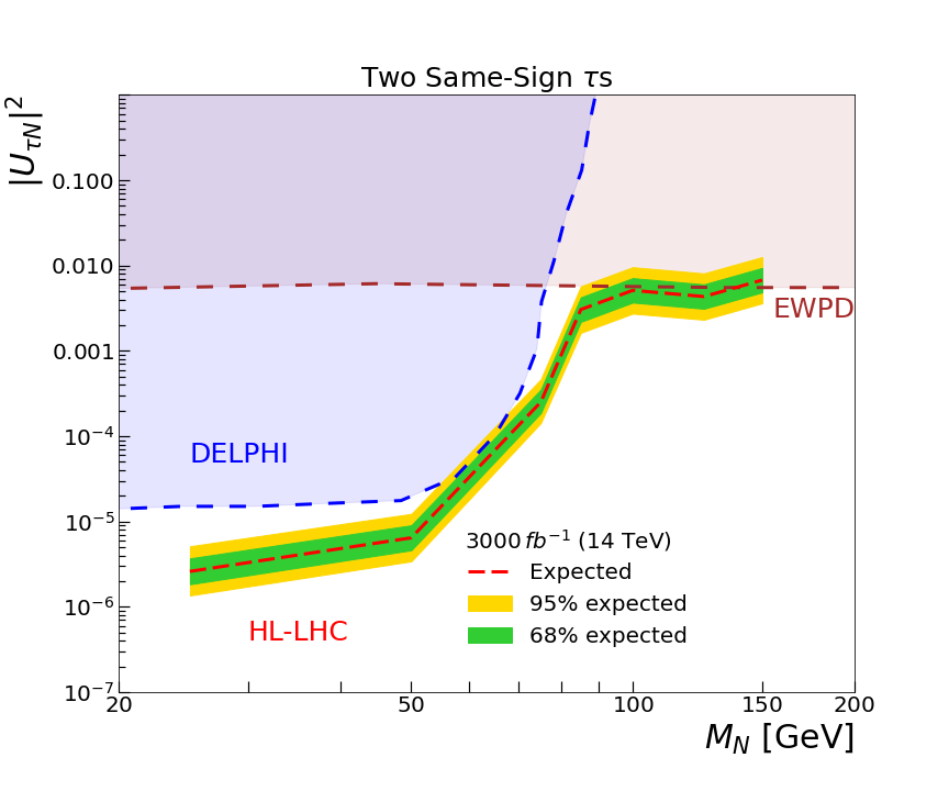
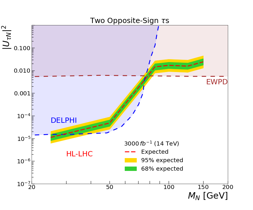
Figure 17: The expected sensitivity reach of $|U_{\tau N}|^{2}$ as a function of the mass $M_{N}$ of the HNL for the same-sign $\tau$ selection (left panel) and opposite-sign $\tau$ selection (right panel) at $\sqrt{s}=14$ TeV with an integrated luminosity $\mathcal{L}=3000fb^{-1}$. The exclusion region at $95\%\ (68\%)$ CL in the $M_{N}$ vs. $|U_{\tau N}|^{2}$ plane is shown in the yellow (green) band. The constraints from EWPD and DELPHI of Fig. 6 are added for comparison.

Finally, the interpretation of our signal-background analysis results at $\sqrt{s}=14$ TeV with an integrated luminosity $\mathcal{L}=3000fb^{-1}$ is presented in the left (right) panel of Fig. 17 for two-same-sign $\tau$ selection (two-opposite-sign $\tau$ selection). The exclusion region at $95\%\,(68\%)$ CL in the $M_{N}$ vs. $|U_{\tau N}|^{2}$ plane is shown in the yellow (green) band. Those SM backgrounds without MLM matching could have some level of theoretical uncertainties coming from higher order corrections as large as $+(50\mathchar 45\relax 100)\%$. Here we take into account these uncertainties by allowing a factor of 2 in the background calculation as a conservative estimation. The constraints from EWPD and DELPHI of Fig. 6 are added for comparison. We estimate the background uncertainties as $\sqrt{B}$ (we consider only the statistical one in this work) in the CLs method Read:2002hq where $B$ is the total background event numbers. Also, the background-only hypothesis is assumed and Gaussian distributions are used for nuisance parameters. The RooStats package Moneta:2010pm is applied to estimate the confident interval with Asymptotic calculator and one-sided Profile Likelihood. We observe that the sensitivity bounds from HL-LHC can be stronger than LEP and EWPD constraints in some parameter space, especially for two-same-sign $\tau$ selection which can reach down to $|U_{\tau N}|^{2}\approx 5\times 10^{-6}$ for $M_{N}\lesssim 50$ GeV. These regions are close to the boundaries between the prompt and long-lived decays of HNLs at the LHC scale. Hence, our study in this paper can serve as a complementary sensitivity reach of Ref. Cottin:2018nms to make HNL searches in the channel $pp\rightarrow W^{\pm(\ast)}+X\rightarrow\tau^{\pm}N+X$ more complete.

VI Conclusions

The puzzle of tiny neutrino masses and the origin of the matter-antimatter asymmetry of the Universe are two vital issues beyond the standard model. Electroweak scale Type-I seesaw mechanism is one of the highly-motivated proposals to explain them simultaneously while maintaining the detectability of the new particles. The model can be tested in present or near-future experiments including the LHC to tell if one or more heavy neutral leptons exist at the electroweak scale. The discovery of heavy neutral leptons will become a concrete evidence of new physics without any doubt.

Among numerous ways to search for heavy neutral leptons in various mass ranges, the LHC can still serve as the most powerful machine to probe $\mathcal{O}(10-100)$ GeV heavy neutral leptons in the present as shown in Figs. 4 and 5. Since there are fewer collider studies of the mixing between $\nu_{\tau}$ and HNL in literature compared with those of $\nu_{e}$ and $\nu_{\mu}$ for the HNL of mass in the electroweak scale as shown in Fig. 6, we focus on the channel $pp\rightarrow W^{\pm(\ast)}+X\rightarrow\tau^{\pm}N+X$ to search for heavy neutral leptons at the LHC 14 TeV in this work.

The targeted signature in this study consists of three prompt charged leptons which includes at least two tau leptons. We further classify our simulations and event selections according to two same-sign $\tau$s or two opposite-sign $\tau$s for revealing the Majorana nature of heavy neutral leptons. After the signal-background analysis, we can observe these event selections can pick out most parts of the signal against SM backgrounds, especially for the $M_{N}<m_{W}$ benchmark points as shown in Tables 1 and 3 and Figs. 10, 14. We summarize our predictions for the testable bounds from HL-LHC in Fig. 17 which is stronger than the previous LEP constraint and Electroweak Precision Data (EWPD). It is obvious that the selection of two same-sign $\tau$s is more powerful than two opposite-sign $\tau$s and it can reach down to $|U_{\tau N}|^{2}\approx 5\times 10^{-6}$ for $M_{N}\lesssim 50$ GeV. We should emphasize even this work is based in the context of $\nu$MSM with Majorana neutrinos, our analysis can also be applied to models with Dirac-like/pseudo-Dirac heavy neutrinos with and without charged lepton flavor violation.

Appendix A Formulas for Heavy Neutral Lepton partial decay widths

For the low mass region ($M_{N}\ll m_{W,Z}$), we follow the calculations in Ref. Atre:2009rg ; Helo:2010cw ; Helo:2013prd for the partial decay widths of $N$. Notice that we consider the inclusive approach, and take the parameter $\mu_{0}\sim m_{\eta^{\prime}}=957.78\pm 0.06$ MeV for the mass threshold from which we start taking into account hadronic contributions via $q\overline{q}$ production.

1. For $N\rightarrow l^{-}_{\alpha}l^{+}_{\beta}\nu_{\beta},N\rightarrow l^{+}_{\alpha}l^{-}_{\beta}\overline{\nu_{l_{\beta}}}$ and $\alpha\neq\beta$

   $$\Gamma(N\rightarrow l^{-}_{\alpha}l^{+}_{\beta}\nu_{\beta}) =\Gamma(N\rightarrow l^{+}_{\alpha}l^{-}_{\beta}\overline{\nu_{\beta}})$$ (14)

   $$=|U_{\alpha N}|^{2}\frac{G_{F}^{2}}{192\pi^{3}}M_{N}^{5}I_{1}(y_{l_{\alpha}},y_{\nu_{\beta}},y_{l_{\beta}})$$

   $$\equiv|U_{\alpha N}|^{2}\Gamma^{(l_{\alpha}l_{\beta}\nu_{\beta})}\,.$$

2. For $N\rightarrow\nu_{\alpha}l^{-}_{\beta}l^{+}_{\beta},N\rightarrow\overline{\nu_{\alpha}}l^{+}_{\beta}l^{-}_{\beta}$

   $$\Gamma(N\rightarrow\nu_{\alpha}l^{-}_{\beta}l^{+}_{\beta}) =\Gamma(N\rightarrow\overline{\nu_{\alpha}}l^{+}_{\beta}l^{-}_{\beta})$$ (15)

   $$=|U_{\alpha N}|^{2}\frac{G_{F}^{2}}{96\pi^{3}}M_{N}^{5}\Big{[}\left(g^{l}_{L}g^{l}_{R}+\delta_{l_{\alpha}l_{\beta}}g^{l}_{R}\right)I_{2}\left(y_{\nu_{\alpha}},y_{l_{\beta}},y_{l_{\beta}}\right)$$

   $$+\left(\left(g^{l}_{L}\right)^{2}+\left(g^{l}_{R}\right)^{2}+\delta_{l_{\alpha}l_{\beta}}(1+2g^{l}_{L})\right)I_{1}\left(y_{\nu_{l_{\alpha}}},y_{l_{\beta}},y_{l_{\beta}}\right)\Big{]}$$

   $$\equiv|U_{\alpha N}|^{2}\Gamma^{(\nu_{\alpha}l_{\beta}l_{\beta})}\,.$$

3. For $N\rightarrow\nu_{l_{\alpha}}\nu_{l_{\beta}}\overline{\nu_{l_{\beta}}},N\rightarrow\overline{\nu_{\alpha}}\overline{\nu_{\beta}}\nu_{\beta}$

   $$\sum_{\beta=e,\mu,\tau}\Gamma(N\rightarrow\nu_{\alpha}\nu_{\beta}\overline{\nu_{l_{\beta}}}) =\sum_{\beta=e,\mu,\tau}\Gamma(N\rightarrow\overline{\nu_{\alpha}}\overline{\nu_{\beta}}\nu_{\beta})$$ (16)

   $$=|U_{\alpha N}|^{2}\frac{G_{F}^{2}}{96\pi^{3}}M_{N}^{5}$$

   $$\equiv|U_{\alpha N}|^{2}\Gamma^{(3\nu)}\,.$$

4. For $N\rightarrow l^{-}_{\alpha}U\overline{D},N\rightarrow l^{+}_{\alpha}\overline{U}D$

   $$\Gamma(N\rightarrow l^{-}_{\alpha}U\overline{D}) =\Gamma(N\rightarrow l^{+}_{\alpha}\overline{U}D)$$ (17)

   $$=|U_{\alpha N}|^{2}|V_{UD}|^{2}\frac{G_{F}^{2}}{64\pi^{3}}M_{N}^{5}I_{1}\left(y_{l_{\alpha}},y_{U},y_{D}\right)$$

   $$\equiv|U_{l_{\alpha}N}|^{2}\Gamma^{(lUD)}\,.$$

5. For $N\rightarrow\nu_{\alpha}q\overline{q},N\rightarrow\overline{\nu_{\alpha}}\overline{q}q$

   $$\Gamma(N\rightarrow\nu_{\alpha}q\overline{q}) =\Gamma(N\rightarrow\overline{\nu_{\alpha}}\overline{q}q)$$ (18)

   $$=|U_{\alpha N}|^{2}\frac{G_{F}^{2}}{32\pi^{3}}M_{N}^{5}\Big{[}g^{q}_{L}g^{q}_{R}I_{2}\left(y_{\nu_{\alpha}},y_{q},y_{q}\right)+\left(\left(g^{q}_{L}\right)^{2}+\left(g^{q}_{R}\right)^{2}\right)I_{1}\left(y_{\nu_{\alpha}},y_{q},y_{q}\right)\big{]}$$

   $$\equiv|U_{\alpha N}|^{2}\Gamma^{(\nu qq)}\,.$$

Here we denoted $y_{i}=m_{i}/M_{N}$ with $m_{i}=m_{l,q}$ and $U=u,c$, $D=d,s,b$ and $q=u,d,c,s,b$. For lepton and quark masses, we apply the values from PDG 2018 Tanabashi:2018oca .

The SM neutral current couplings of leptons and quarks are

$$g^{l}_{L} =-\frac{1}{2}+\sin^{2}\theta_{W}\,,\quad q^{U}_{L}=\frac{1}{2}-\frac{2}{3}\sin^{2}\theta_{W}\,,\quad q^{D}_{L}=-\frac{1}{2}+\frac{1}{3}\sin^{2}\theta_{W}\,,$$ (19)

$$g^{l}_{R} =\sin^{2}\theta_{W}\,,\quad q^{U}_{R}=-\frac{2}{3}\sin^{2}\theta_{W}\,,\quad q^{D}_{R}=\frac{1}{3}\sin^{2}\theta_{W}\,.$$

The kinematical functions used above are

$$\lambda(x,y,z) =x^{2}+y^{2}+z^{2}-2xy-2yz-2xz\,,$$ (20)

$$I_{1}(x,y,z) =12\int^{(1-z)^{2}}_{(x+y)^{2}}\frac{ds}{s}(s-x^{2}-y^{2})(1+z^{2}-s)\lambda^{1/2}(s,x^{2},y^{2})\lambda^{1/2}(1,s,z^{2})\,,$$ (21)

$$I_{2}(x,y,z) =24yz\int^{(1-x)^{2}}_{(y+z)^{2}}\frac{ds}{s}(1+x^{2}-s)\lambda^{1/2}(s,y^{2},z^{2})\lambda^{1/2}(1,s,x^{2})\,.$$ (22)

For the medium mass region ($M_{N}\lesssim m_{t}$), we take into account the both effects of on-shell and off-shell $W$ and $Z$ bosons by including the width of these gauge bosons in the propagators. We follow the calculations in Ref. Atre:2009rg ; Liao:2017jiz for the the partial decay widths of $N$. Notice all the SM fermion masses of the final states have been neglected to simplify our calculations.

1. For $N\rightarrow l^{-}_{\alpha}l^{+}_{\beta}\nu_{\beta},N\rightarrow l^{+}_{\alpha}l^{-}_{\beta}\overline{\nu_{\beta}}$ and $\alpha\neq\beta$

   $$\Gamma(N\rightarrow l^{-}_{\alpha}l^{+}_{\beta}\nu_{\beta}) =\Gamma(N\rightarrow l^{+}_{\alpha}l^{-}_{\beta}\overline{\nu_{\beta}})$$ (23)

   $$=|U_{\alpha N}|^{2}F_{N}\left(M_{N},m_{W},\Gamma_{W}\right)$$

   $$\equiv|U_{l_{1}N}|^{2}\Gamma^{(l_{1}l_{2}\nu)}\,.$$

2. For $N\rightarrow\nu_{\alpha}l^{-}_{\beta}l^{+}_{\beta},N\rightarrow\overline{\nu_{\alpha}}l^{+}_{\beta}l^{-}_{\beta}$

   $$\Gamma(N\rightarrow\nu_{\alpha}l^{-}_{\beta}l^{+}_{\beta}) =\Gamma(N\rightarrow\overline{\nu_{\alpha}}l^{+}_{\beta}l^{-}_{\beta})$$ (24)

   $$=|U_{\alpha N}|^{2}\Big{[}F_{N}\left(M_{N},m_{W},\Gamma_{W}\right)+3\left(\left(g^{l}_{L}\right)^{2}+\left(g^{l}_{R}\right)^{2}\right)F_{N}\left(M_{N},m_{Z},\Gamma_{Z}\right)$$

   $$+2g^{l}_{L}F_{S}\left(M_{N},m_{W},\Gamma_{W},m_{Z},\Gamma_{Z}\right)\Big{]}$$

   $$\equiv|U_{\alpha N}|^{2}\Gamma^{(l_{2}l_{2}\nu)}\,.$$

3. For $N\rightarrow\nu_{\alpha}\nu_{\beta}\overline{\nu_{\beta}},N\rightarrow\overline{\nu_{\alpha}}\overline{\nu_{\beta}}\nu_{\beta}$

   $$\sum_{\beta=e,\mu,\tau}\Gamma(N\rightarrow\nu_{\alpha}\nu_{\beta}\overline{\nu_{\beta}}) =\sum_{\beta=e,\mu,\tau}\Gamma(N\rightarrow\overline{\nu_{\alpha}}\overline{\nu_{\beta}}\nu_{\beta})$$ (25)

   $$=|U_{\alpha N}|^{2}\frac{1}{4}(2+4)F_{N}\left(M_{N},m_{Z},\Gamma_{Z}\right)$$

   $$\equiv|U_{\alpha N}|^{2}\Gamma^{(3\nu)}\,.$$

4. For $N\rightarrow l^{-}_{\alpha}U\overline{D},N\rightarrow l^{+}_{\alpha}\overline{U}D$

   $$\Gamma(N\rightarrow l^{-}_{\alpha}U\overline{D}) =\Gamma(N\rightarrow l^{+}_{\alpha}\overline{U}D)$$ (26)

   $$=|U_{\alpha N}|^{2}|V_{UD}|^{2}N_{c}F_{N}\left(M_{N},m_{W},\Gamma_{W}\right)$$

   $$\equiv|U_{\alpha N}|^{2}\Gamma^{(lUD)}\,.$$

5. For $N\rightarrow\nu_{\alpha}q\overline{q},N\rightarrow\overline{\nu_{l_{\alpha}}}\overline{q}q$

   $$\Gamma(N\rightarrow\nu_{\alpha}q\overline{q}) =\Gamma(N\rightarrow\overline{\nu_{\alpha}}\overline{q}q)$$ (27)

   $$=|U_{\alpha N}|^{2}N_{c}\left(\left(g^{q}_{L}\right)^{2}+\left(g^{q}_{R}\right)^{2}\right)F_{N}\left(M_{N},m_{Z},\Gamma_{Z}\right)$$

   $$\equiv|U_{\alpha N}|^{2}\Gamma^{(\nu qq)}\,.$$

where $N_{c}=3$ is the number of color degrees of freedom for quarks.

The functions $F_{N}$ is

$$F_{N}\left(M_{N},m_{W},\Gamma_{W}\right)=\frac{G^{2}_{F}M_{N}}{\pi^{3}}\int^{\frac{M_{N}}{2}}_{0}dE_{1}\int^{\frac{M_{N}}{2}}_{\frac{M_{N}}{2}-E_{1}}\left(|P_{W}|^{2}\frac{1}{2}\left(M_{N}-2E_{2}\right)E_{2}\right)dE_{2}\,,$$ (28)

where $P_{W}$ comes from the propagator of the $W$ boson with the form,

$$P_{W}=\frac{m^{2}_{W}}{q^{2}-m^{2}_{W}+i\Gamma_{W}m_{W}}\,,$$ (29)

where $q^{2}=M^{2}_{N}-2M_{N}E_{1}$ and $\Gamma_{W}$ is the total decay width of $W$. We can simply obtain $F_{N}(M_{N},m_{Z},\Gamma_{Z})$ by taking $(m_{W},\Gamma_{W})\rightarrow(m_{Z},\Gamma_{Z})$.

On the other hand, the function $F_{S}$ is given by

$$F_{S}=\frac{G^{2}_{F}M_{N}}{\pi^{3}}\int^{\frac{M_{N}}{2}}_{0}dE_{1}\int^{\frac{M_{N}}{2}}_{\frac{M_{N}}{2}-E_{1}}\left(\left(P_{W}P^{\ast}_{Z}+P^{\ast}_{W}P_{Z}\right)\frac{1}{2}\left(M_{N}-2E_{2}\right)E_{2}\right)dE_{2}\,,$$ (30)

and $P_{Z}$ comes from the propagator of the $Z$ boson with the form,

$$P_{Z}=\frac{m^{2}_{Z}}{q^{2}_{3}-m^{2}_{Z}+i\Gamma_{Z}m_{Z}}\,,$$ (31)

where $q^{2}_{3}=M^{2}_{N}-2M_{N}E_{3}$ with $E_{3}=M_{N}-E_{1}-E_{2}$ considering the decay of $N$ at rest.

Besides, we also take into account the $N$ partial decay width to the Higgs boson and an active neutrino when $N$ is heavier than the Higgs boson,

$$\Gamma(N\rightarrow\nu_{\alpha}H) =\frac{g^{2}}{64\pi m^{2}_{W}}|U_{\alpha N}|^{2}M^{3}_{N}\left(1-\frac{m^{2}_{H}}{M^{2}_{N}}\right)^{2}$$ (32)

$$\equiv|U_{\alpha N}|^{2}\Gamma^{(\nu H)}\,.$$ (33)

Finally, we represent the total decay width of $N$ as

$$\Gamma_{N} =\sum_{\alpha,\beta,\mathcal{H}}\Big{[}2\times\Gamma(N\rightarrow l^{-}_{\alpha}\mathcal{H}^{+})+2\times\Gamma(N\rightarrow l^{-}_{\alpha}l^{+}_{\beta}\nu_{\beta})+\Gamma(N\rightarrow\nu_{\beta}\mathcal{H}^{0})$$ (34)

$$+\Gamma(N\rightarrow l^{-}_{\beta}l^{+}_{\beta}\nu_{\alpha})+\Gamma(N\rightarrow\nu_{\alpha}\nu_{\beta}\overline{\nu_{\beta}})\Big{]}+\Gamma(N\rightarrow\nu_{\alpha}H)\,,$$ (35)

where we denoted the hadronic states $\mathcal{H}^{+}=\overline{d}u,\overline{s}u,\overline{d}c,\overline{s}c,\overline{b}u,\overline{b}c$ and $\mathcal{H}^{0}=\overline{q}q$. Then we further simplify $\Gamma_{N}$ as

$$\Gamma_{N}=a_{e}(M_{N})\cdot|U_{eN}|^{2}+a_{\mu}(M_{N})\cdot|U_{\mu N}|^{2}+a_{\tau}(M_{N})\cdot|U_{\tau N}|^{2}\,,$$ (36)

where

$$a_{\alpha}(M_{N})=2\times\Gamma^{(l_{\alpha}\mathcal{H})}+\Gamma^{(\nu\mathcal{H})}+\Gamma^{(3\nu)}+\sum_{\beta}\left(\Gamma^{(l_{\beta}l_{\beta}\nu)}+2\times\Gamma^{(l_{\alpha}l_{\beta}\nu)}\right)+\Gamma^{(\nu H)}\,,$$ (37)

with $\alpha,\beta=e,\mu,\tau$.

Appendix B Extra cut flow tables and kinematical distributions

Two Same-Sign $\tau$s Selection Flow Table
Process	$\sigma$	Preselection	$P_{T}^{miss}<$ 40 GeV	b veto	Invariant Mass Selection
	(fb)	$A\epsilon$ (%)	$A\epsilon$ (%)	$A\epsilon$ (%)	$A\epsilon$ (%)
$M_{N}$ = 25 GeV	$2.851$	$2.535$	$2.348$	$2.289$	$1.640$
$W^{\pm}W^{\pm}W^{\mp}$	$1.828\times 10^{-1}$	$1.331$	$7.078\times 10^{-1}$	$6.935\times 10^{-1}$	$5.280\times 10^{-2}$
$W^{+}W^{-}Z/H/\gamma$	$1.065\times 10^{-1}$	$8.680\times 10^{-1}$	$4.174\times 10^{-1}$	$4.085\times 10^{-1}$	$3.785\times 10^{-2}$
$t\bar{t}+nj$	$2.357\times 10^{4}$	$6.471\times 10^{-2}$	$1.287\times 10^{-2}$	$1.759\times 10^{-3}$	$9.637\times 10^{-5}$
Process	$\sigma$	Preselection	$P_{T}^{miss}<$ 40 GeV	b veto	Invariant Mass Selection
	(fb)	$A\epsilon$ (%)	$A\epsilon$ (%)	$A\epsilon$ (%)	$A\epsilon$ (%)
$M_{N}$ = 50 GeV	$2.068$	$2.931$	$2.683$	$2.612$	$2.368$
$W^{\pm}W^{\pm}W^{\mp}$	$1.828\times 10^{-1}$	$1.331$	$7.078\times 10^{-1}$	$6.935\times 10^{-1}$	$1.628\times 10^{-1}$
$W^{+}W^{-}Z/H/\gamma$	$1.065\times 10^{-1}$	$8.680\times 10^{-1}$	$4.174\times 10^{-1}$	$4.085\times 10^{-1}$	$1.129\times 10^{-1}$
$t\bar{t}+nj$	$2.357\times 10^{4}$	$6.471\times 10^{-2}$	$1.287\times 10^{-2}$	$1.759\times 10^{-3}$	$3.373\times 10^{-4}$
Process	$\sigma$	Preselection	$P_{T}^{miss}<$ 40 GeV	b veto	Invariant Mass Selection
	(fb)	$A\epsilon$ (%)	$A\epsilon$ (%)	$A\epsilon$ (%)	$A\epsilon$ (%)
$M_{N}$ = 75 GeV	$8.935\times 10^{-2}$	$1.588$	$1.302$	$1.270$	$8.049\times 10^{-1}$
$W^{\pm}W^{\pm}W^{\mp}$	$1.828\times 10^{-1}$	$1.331$	$7.078\times 10^{-1}$	$6.935\times 10^{-1}$	$1.787\times 10^{-1}$
$W^{+}W^{-}Z/H/\gamma$	$1.065\times 10^{-1}$	$8.680\times 10^{-1}$	$4.174\times 10^{-1}$	$4.085\times 10^{-1}$	$1.231\times 10^{-1}$
$t\bar{t}+nj$	$2.357\times 10^{4}$	$6.471\times 10^{-2}$	$1.287\times 10^{-2}$	$1.759\times 10^{-3}$	$4.337\times 10^{-4}$

Table 5: The same as Table 1 except for the change of $15<P^{\tau_{1}(\tau_{2})}_{T}<50(30)\;{\rm GeV}$ in Preselection.

Two Opposite-Sign $\tau$s Selection Flow Table
Process	$\sigma$	Preselection	$P_{T}^{miss}<$ 40 GeV	b veto	Invariant Mass Selection
	(fb)	$A\epsilon$ (%)	$A\epsilon$ (%)	$A\epsilon$ (%)	$A\epsilon$ (%)
$M_{N}$ = 25 GeV	$2.291$	$1.808$	$1.627$	$1.591$	$1.432$
$W^{\pm}Z/H/\gamma$	$1.599\times 10^{2}$	$6.689\times 10^{-1}$	$5.146\times 10^{-1}$	$5.059\times 10^{-1}$	$3.080\times 10^{-2}$
$ZZ/\gamma$	$2.400\times 10^{1}$	$6.681\times 10^{-1}$	$5.859\times 10^{-1}$	$5.791\times 10^{-1}$	$6.070\times 10^{-2}$
$\tau\tau+nj$	$9.559\times 10^{5}$	$3.067\times 10^{-4}$	$3.067\times 10^{-4}$	$3.067\times 10^{-4}$	$2.045\times 10^{-5}$
$t\bar{t}+nj$	$2.987\times 10^{4}$	$2.560\times 10^{-2}$	$4.994\times 10^{-3}$	$5.660\times 10^{-4}$	$4.043\times 10^{-5}$
Process	$\sigma$	Preselection	$P_{T}^{miss}<$ 40 GeV	b veto	Invariant Mass Selection
	(fb)	$A\epsilon$ (%)	$A\epsilon$ (%)	$A\epsilon$ (%)	$A\epsilon$ (%)
$M_{N}$ = 50 GeV	$2.052$	$1.595$	$1.431$	$1.396$	$1.322$
$W^{\pm}Z/H/\gamma$	$1.599\times 10^{2}$	$6.689\times 10^{-1}$	$5.146\times 10^{-1}$	$5.059\times 10^{-1}$	$1.029\times 10^{-1}$
$ZZ/\gamma$	$2.400\times 10^{1}$	$6.681\times 10^{-1}$	$5.859\times 10^{-1}$	$5.791\times 10^{-1}$	$1.439\times 10^{-1}$
$\tau\tau+nj$	$9.559\times 10^{5}$	$3.067\times 10^{-4}$	$3.067\times 10^{-4}$	$3.067\times 10^{-4}$	$1.022\times 10^{-4}$
$t\bar{t}+nj$	$2.987\times 10^{4}$	$2.560\times 10^{-2}$	$4.994\times 10^{-3}$	$5.660\times 10^{-4}$	$2.022\times 10^{-4}$
Process	$\sigma$	Preselection	$P_{T}^{miss}<$ 40 GeV	b veto	Invariant Mass Selection
	(fb)	$A\epsilon$ (%)	$A\epsilon$ (%)	$A\epsilon$ (%)	$A\epsilon$ (%)
$M_{N}$ = 75 GeV	$9.104\times 10^{-2}$	$7.987\times 10^{-1}$	$6.439\times 10^{-1}$	$6.279\times 10^{-1}$	$4.506\times 10^{-1}$
$W^{\pm}Z/H/\gamma$	$1.599\times 10^{2}$	$6.689\times 10^{-1}$	$5.146\times 10^{-1}$	$5.059\times 10^{-1}$	$1.125\times 10^{-1}$
$ZZ/\gamma$	$2.400\times 10^{1}$	$6.681\times 10^{-1}$	$5.859\times 10^{-1}$	$5.791\times 10^{-1}$	$1.538\times 10^{-1}$
$\tau\tau+nj$	$9.559\times 10^{5}$	$3.067\times 10^{-4}$	$3.067\times 10^{-4}$	$3.067\times 10^{-4}$	$1.431\times 10^{-4}$
$t\bar{t}+nj$	$2.987\times 10^{4}$	$2.560\times 10^{-2}$	$4.994\times 10^{-3}$	$5.660\times 10^{-4}$	$2.426\times 10^{-4}$

Table 6: The same as Table 3 except for the change of $15<P^{\tau_{1}(\tau_{2})}_{T}<50(30)\;{\rm GeV}$ in Preselection.

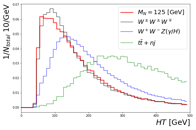
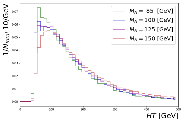
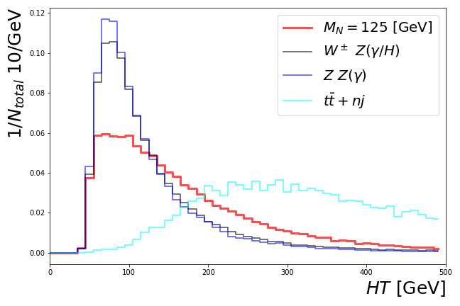
Figure 18: The inclusive $H_{T}$ distributons for the same-sign $\tau$ selection (upper panel) and opposite-sign $\tau$ selection (lower panel). Notice all distributions passed the preselection criteria.

In this appendix, we collect some extra cut flow tables and kinematical distributions which are not shown in the main text. First, inspired from the Ref. Florez:2016lwi ; Aboubrahim:2017aen , the situation with $15<P^{\tau_{1}(\tau_{2})}_{T}<50(30)\;{\rm GeV}$ may also be possible for $M_{N}<m_{W}$ and this selection can enhance the signal sensitivity reach. Therefore, we list this kind of event slection for the two same-sign $\tau$s selection flow table in Table 5 and two opposite-sign $\tau$s selection flow table in Table 6 for readers as a reference. Second, in order to remove the extra hadronic activity from SM backgrounds for $M_{N}>m_{W}$, the inclusive scalar sum of jet $E_{T}$, $H_{T}$, which is defined in Eq. (5.20) of Ref. Pascoli:2018heg is applied in our analysis. The inclusive $H_{T}$ distributons are shown in Fig. 18 for the same-sign $\tau$ selection (upper panel) and opposite-sign $\tau$ selection (lower panel). The selection $H_{T}<200\;{\rm GeV}$ can effectively reduce the hadronic activity from $t\overline{t}$ associated processes.

References

- (1) P. Minkowski, Phys. Lett. 67B, 421 (1977). doi:10.1016/0370-2693(77)90435-X
- (2) T. Yanagida, Conf. Proc. C 7902131, 95 (1979).
- (3) T. Yanagida, Prog. Theor. Phys. 64, 1103 (1980). doi:10.1143/PTP.64.1103
- (4) M. Gell-Mann, P. Ramond and R. Slansky, Conf. Proc. C 790927, 315 (1979) [arXiv:1306.4669 [hep-th]].
- (5) P. Ramond, in Talk given at the Sanibel Symposium, Palm Coast, Fla., Feb. 25-Mar. 2, 1979, preprint CALT-68-709 (retroprinted as hep-ph/9809459).
- (6) S. L. Glashow, in Proc. of the Cargése Summer Institute on Quarks and Leptons, Cargése, July 9-29, 1979, eds. M. Lévy et. al, , (Plenum, 1980, New York), p707.
- (7) R. N. Mohapatra and G. Senjanovic, Phys. Rev. Lett. 44, 912 (1980). doi:10.1103/PhysRevLett.44.912
- (8) M. Fukugita and T. Yanagida, Phys. Lett. B 174, 45 (1986). doi:10.1016/0370-2693(86)91126-3
- (9) S. Davidson and A. Ibarra, Phys. Lett. B 535, 25 (2002) doi:10.1016/S0370-2693(02)01735-5 [hep-ph/0202239].
- (10) O. Ruchayskiy and A. Ivashko, JCAP 1210, 014 (2012) doi:10.1088/1475-7516/2012/10/014 [arXiv:1202.2841 [hep-ph]].
- (11) T. Asaka, S. Blanchet and M. Shaposhnikov, Phys. Lett. B 631, 151 (2005) doi:10.1016/j.physletb.2005.09.070 [hep-ph/0503065].
- (12) T. Asaka and M. Shaposhnikov, Phys. Lett. B 620, 17 (2005) doi:10.1016/j.physletb.2005.06.020 [hep-ph/0505013].
- (13) E. K. Akhmedov, V. A. Rubakov and A. Y. Smirnov, Phys. Rev. Lett. 81, 1359 (1998) doi:10.1103/PhysRevLett.81.1359 [hep-ph/9803255].
- (14) R. E. Shrock, Phys. Lett. 96B, 159 (1980). doi:10.1016/0370-2693(80)90235-X
- (15) R. E. Shrock, Phys. Rev. D 24, 1232 (1981). doi:10.1103/PhysRevD.24.1232
- (16) R. E. Shrock, Phys. Rev. D 24, 1275 (1981). doi:10.1103/PhysRevD.24.1275
- (17) A. Atre, T. Han, S. Pascoli and B. Zhang, JHEP 0905, 030 (2009) doi:10.1088/1126-6708/2009/05/030 [arXiv:0901.3589 [hep-ph]].
- (18) T. Asaka, S. Eijima and H. Ishida, JHEP 1104, 011 (2011) doi:10.1007/JHEP04(2011)011 [arXiv:1101.1382 [hep-ph]].
- (19) T. Asaka and H. Ishida, Phys. Lett. B 763, 393 (2016) doi:10.1016/j.physletb.2016.10.070 [arXiv:1609.06113 [hep-ph]].
- (20) A. Abada, C. Hati, X. Marcano and A. M. Teixeira, JHEP 1909, 017 (2019) doi:10.1007/JHEP09(2019)017 [arXiv:1904.05367 [hep-ph]].
- (21) E. J. Chun, A. Das, S. Mandal, M. Mitra and N. Sinha, Phys. Rev. D 100, no. 9, 095022 (2019) doi:10.1103/PhysRevD.100.095022 [arXiv:1908.09562 [hep-ph]].
- (22) D. A. Bryman and R. Shrock, Phys. Rev. D 100, 073011 (2019) doi:10.1103/PhysRevD.100.073011 [arXiv:1909.11198 [hep-ph]].
- (23) J. Kersten and A. Y. Smirnov, Phys. Rev. D 76, 073005 (2007) doi:10.1103/PhysRevD.76.073005 [arXiv:0705.3221 [hep-ph]].
- (24) A. Blondel et al. [FCC-ee study Team], Nucl. Part. Phys. Proc. 273-275, 1883 (2016) doi:10.1016/j.nuclphysbps.2015.09.304 [arXiv:1411.5230 [hep-ex]].
- (25) F. F. Deppisch, P. S. Bhupal Dev and A. Pilaftsis, New J. Phys. 17, no. 7, 075019 (2015) doi:10.1088/1367-2630/17/7/075019 [arXiv:1502.06541 [hep-ph]].
- (26) M. Drewes, B. Garbrecht, D. Gueter and J. Klaric, JHEP 1708, 018 (2017) doi:10.1007/JHEP08(2017)018 [arXiv:1609.09069 [hep-ph]].
- (27) Y. Cai, T. Han, T. Li and R. Ruiz, Front. in Phys. 6, 40 (2018) doi:10.3389/fphy.2018.00040 [arXiv:1711.02180 [hep-ph]].
- (28) J. C. Helo, M. Hirsch and Z. S. Wang, JHEP 1807, 056 (2018) doi:10.1007/JHEP07(2018)056 [arXiv:1803.02212 [hep-ph]].
- (29) N. Liu, Z. G. Si, L. Wu, H. Zhou and B. Zhu, Phys. Rev. D 101, no. 7, 071701 (2020) doi:10.1103/PhysRevD.101.071701 [arXiv:1910.00749 [hep-ph]].
- (30) K. Bondarenko, A. Boyarsky, D. Gorbunov and O. Ruchayskiy, JHEP 11 (2018), 032 doi:10.1007/JHEP11(2018)032 [arXiv:1805.08567 [hep-ph]].
- (31) G. Cvetič and C. S. Kim, Phys. Rev. D 100, no. 1, 015014 (2019) doi:10.1103/PhysRevD.100.015014 [arXiv:1904.12858 [hep-ph]].
- (32) A. Abada, N. Bernal, M. Losada and X. Marcano, JHEP 1901, 093 (2019) doi:10.1007/JHEP01(2019)093 [arXiv:1807.10024 [hep-ph]].
- (33) G. Cottin, J. C. Helo and M. Hirsch, Phys. Rev. D 98, no. 3, 035012 (2018) doi:10.1103/PhysRevD.98.035012 [arXiv:1806.05191 [hep-ph]].
- (34) P. Hernández, J. Jones-Pérez and O. Suarez-Navarro, Eur. Phys. J. C 79 (2019) no.3, 220 doi:10.1140/epjc/s10052-019-6728-1 [arXiv:1810.07210 [hep-ph]].
- (35) M. Drewes, A. Giammanco, J. Hajer and M. Lucente, Phys. Rev. D 101 (2020) no.5, 055002 doi:10.1103/PhysRevD.101.055002 [arXiv:1905.09828 [hep-ph]].
- (36) A. Flórez, K. Gui, A. Gurrola, C. Patiño and D. Restrepo, Phys. Lett. B 778, 94 (2018) doi:10.1016/j.physletb.2018.01.009 [arXiv:1708.03007 [hep-ph]].
- (37) S. Pascoli, R. Ruiz and C. Weiland, Phys. Lett. B 786, 106 (2018) doi:10.1016/j.physletb.2018.08.060 [arXiv:1805.09335 [hep-ph]].
- (38) M. Gronau, C. N. Leung and J. L. Rosner, Phys. Rev. D 29 (1984), 2539 doi:10.1103/PhysRevD.29.2539
- (39) M. L. Perl, T. Barklow, A. Boyarski, M. Breidenbach, P. Burchat, D. L. Burke, J. Dorfan, G. J. Feldman, L. D. Gladney, G. Hanson, K. G. Hayes, R. J. Hollebeek, W. R. Innes, J. Jaros, D. Karlen, A. J. Lankford, R. R. Larsen, B. LeClaire, N. Lockyer, V. Luth, C. Matteuzzi, R. A. Ong, B. Richter, K. Riles, M. C. Ross, D. Schlatter, J. M. Yelton, C. Zaiser, G. S. Abrams, D. Amidei, A. R. Baden, J. Boyer, F. Butler, G. Gidal, M. S. Gold, G. Goldhaber, L. Golding, J. Haggerty, D. Herrup, I. Juricic, J. A. Kadyk, M. E. Nelson, P. C. Rowson, H. Schellman, W. B. Schmidke, P. D. Sheldon, C. de la Vaissiere, D. R. Wood, M. E. Levi and T. Schaad, Phys. Rev. D 32 (1985), 2859 doi:10.1103/PhysRevD.32.2859
- (40) F. J. Gilman and S. H. Rhie, Phys. Rev. D 32 (1985), 324-326 doi:10.1103/PhysRevD.32.324
- (41) F. J. Gilman, Comments Nucl. Part. Phys. 16 (1986) no.5, 231-247 SLAC-PUB-3898.
- (42) K. Hagiwara and S. Komamiya, Adv. Ser. Direct. High Energy Phys. 1 (1988), 785-859 doi:10.1142/9789814415613_0013
- (43) M. Dittmar, A. Santamaria, M. C. Gonzalez-Garcia and J. W. F. Valle, Nucl. Phys. B 332, 1 (1990). doi:10.1016/0550-3213(90)90028-C
- (44) E. Ma and J. T. Pantaleone, Phys. Rev. D 40, 2172 (1989). doi:10.1103/PhysRevD.40.2172
- (45) D. A. Dicus and P. Roy, Phys. Rev. D 44, 1593 (1991). doi:10.1103/PhysRevD.44.1593
- (46) E. J. Chun et al., Int. J. Mod. Phys. A 33, no. 05n06, 1842005 (2018) doi:10.1142/S0217751X18420058 [arXiv:1711.02865 [hep-ph]].
- (47) D. Alva, T. Han and R. Ruiz, JHEP 1502, 072 (2015) doi:10.1007/JHEP02(2015)072 [arXiv:1411.7305 [hep-ph]].
- (48) S. Pascoli, R. Ruiz and C. Weiland, JHEP 1906, 049 (2019) doi:10.1007/JHEP06(2019)049 [arXiv:1812.08750 [hep-ph]].
- (49) S. Alekhin et al., Rept. Prog. Phys. 79, no. 12, 124201 (2016) doi:10.1088/0034-4885/79/12/124201 [arXiv:1504.04855 [hep-ph]].
- (50) F. Kling and S. Trojanowski, Phys. Rev. D 97, no. 9, 095016 (2018) doi:10.1103/PhysRevD.97.095016 [arXiv:1801.08947 [hep-ph]].
- (51) D. Curtin et al., Rept. Prog. Phys. 82, no. 11, 116201 (2019) doi:10.1088/1361-6633/ab28d6 [arXiv:1806.07396 [hep-ph]].
- (52) L. Lee, C. Ohm, A. Soffer and T. T. Yu, Prog. Part. Nucl. Phys. 106, 210 (2019) doi:10.1016/j.ppnp.2019.02.006 [arXiv:1810.12602 [hep-ph]].
- (53) D. Dercks, H. K. Dreiner, M. Hirsch and Z. S. Wang, Phys. Rev. D 99, no. 5, 055020 (2019) doi:10.1103/PhysRevD.99.055020 [arXiv:1811.01995 [hep-ph]].
- (54) J. Alimena et al., arXiv:1903.04497 [hep-ex].
- (55) G. Aielli et al., arXiv:1911.00481 [hep-ex].
- (56) M. Hirsch and Z. S. Wang, Phys. Rev. D 101, no. 5, 055034 (2020) doi:10.1103/PhysRevD.101.055034 [arXiv:2001.04750 [hep-ph]].
- (57) F. del Aguila, J. de Blas and M. Perez-Victoria, Phys. Rev. D 78, 013010 (2008) doi:10.1103/PhysRevD.78.013010 [arXiv:0803.4008 [hep-ph]].
- (58) E. Akhmedov, A. Kartavtsev, M. Lindner, L. Michaels and J. Smirnov, JHEP 1305, 081 (2013) doi:10.1007/JHEP05(2013)081 [arXiv:1302.1872 [hep-ph]].
- (59) L. Basso, O. Fischer and J. J. van der Bij, EPL 105, no. 1, 11001 (2014) doi:10.1209/0295-5075/105/11001 [arXiv:1310.2057 [hep-ph]].
- (60) J. de Blas, EPJ Web Conf. 60, 19008 (2013) doi:10.1051/epjconf/20136019008 [arXiv:1307.6173 [hep-ph]].
- (61) S. Antusch and O. Fischer, JHEP 1505, 053 (2015) doi:10.1007/JHEP05(2015)053 [arXiv:1502.05915 [hep-ph]].
- (62) O. Adriani et al. [L3 Collaboration], Phys. Lett. B 295, 371 (1992). doi:10.1016/0370-2693(92)91579-X
- (63) M. Acciarri et al. [L3 Collaboration], Phys. Lett. B 461, 397 (1999) doi:10.1016/S0370-2693(99)00852-7 [hep-ex/9909006].
- (64) P. Achard et al. [L3 Collaboration], Phys. Lett. B 517, 67 (2001) doi:10.1016/S0370-2693(01)00993-5 [hep-ex/0107014].
- (65) P. Abreu et al. [DELPHI Collaboration], Z. Phys. C 74, 57 (1997) Erratum: [Z. Phys. C 75, 580 (1997)]. doi:10.1007/s002880050370
- (66) A. M. Sirunyan et al. [CMS Collaboration], Phys. Rev. Lett. 120, no. 22, 221801 (2018) doi:10.1103/PhysRevLett.120.221801 [arXiv:1802.02965 [hep-ex]].
- (67) A. M. Sirunyan et al. [CMS Collaboration], JHEP 1901, 122 (2019) doi:10.1007/JHEP01(2019)122 [arXiv:1806.10905 [hep-ex]].
- (68) G. Aad et al. [ATLAS Collaboration], JHEP 1910, 265 (2019) doi:10.1007/JHEP10(2019)265 [arXiv:1905.09787 [hep-ex]].
- (69) M. Tanabashi et al. [Particle Data Group], Phys. Rev. D 98, no. 3, 030001 (2018). doi:10.1103/PhysRevD.98.030001
- (70) C. Degrande, O. Mattelaer, R. Ruiz and J. Turner, Phys. Rev. D 94, no. 5, 053002 (2016) doi:10.1103/PhysRevD.94.053002 [arXiv:1602.06957 [hep-ph]].
- (71) A. Alloul, N. D. Christensen, C. Degrande, C. Duhr and B. Fuks, Comput. Phys. Commun. 185, 2250 (2014) doi:10.1016/j.cpc.2014.04.012 [arXiv:1310.1921 [hep-ph]].
- (72) J. Alwall et al., JHEP 1407, 079 (2014) doi:10.1007/JHEP07(2014)079 [arXiv:1405.0301 [hep-ph]].
- (73) R. Frederix, S. Frixione, V. Hirschi, D. Pagani, H.-S. Shao and M. Zaro, JHEP 1807, 185 (2018) doi:10.1007/JHEP07(2018)185 [arXiv:1804.10017 [hep-ph]].
- (74) W. Y. Keung and G. Senjanovic, Phys. Rev. Lett. 50, 1427 (1983). doi:10.1103/PhysRevLett.50.1427
- (75) A. Das, P. Konar and A. Thalapillil, JHEP 1802, 083 (2018) doi:10.1007/JHEP02(2018)083 [arXiv:1709.09712 [hep-ph]].
- (76) A. Das, S. Jana, S. Mandal and S. Nandi, Phys. Rev. D 99, no. 5, 055030 (2019) doi:10.1103/PhysRevD.99.055030 [arXiv:1811.04291 [hep-ph]].
- (77) T. Sjostrand, S. Mrenna and P. Z. Skands, Comput. Phys. Commun. 178, 852 (2008) doi:10.1016/j.cpc.2008.01.036 [arXiv:0710.3820 [hep-ph]].
- (78) J. de Favereau et al. [DELPHES 3 Collaboration], JHEP 1402, 057 (2014) doi:10.1007/JHEP02(2014)057 [arXiv:1307.6346 [hep-ex]].
- (79) M. L. Mangano, M. Moretti, F. Piccinini and M. Treccani, JHEP 0701, 013 (2007) doi:10.1088/1126-6708/2007/01/013 [hep-ph/0611129].
- (80) J. Alwall et al., Eur. Phys. J. C 53, 473 (2008) doi:10.1140/epjc/s10052-007-0490-5 [arXiv:0706.2569 [hep-ph]].
- (81) M. Cacciari, G. P. Salam and G. Soyez, JHEP 0804, 063 (2008) doi:10.1088/1126-6708/2008/04/063 [arXiv:0802.1189 [hep-ph]].
- (82) M. Cacciari, G. P. Salam and G. Soyez, Eur. Phys. J. C 72, 1896 (2012) doi:10.1140/epjc/s10052-012-1896-2 [arXiv:1111.6097 [hep-ph]].
- (83) The ATLAS collaboration [ATLAS Collaboration], ATL-PHYS-PUB-2019-033.
- (84) G. Aad et al. [ATLAS Collaboration], Phys. Rev. D 101, no. 5, 052005 (2020) doi:10.1103/PhysRevD.101.052005 [arXiv:1911.12606 [hep-ex]].
- (85) A. Flórez, L. Bravo, A. Gurrola, C. Ávila, M. Segura, P. Sheldon and W. Johns, Phys. Rev. D 94, no. 7, 073007 (2016) doi:10.1103/PhysRevD.94.073007 [arXiv:1606.08878 [hep-ph]].
- (86) A. Aboubrahim, P. Nath and A. B. Spisak, Phys. Rev. D 95, no. 11, 115030 (2017) doi:10.1103/PhysRevD.95.115030 [arXiv:1704.04669 [hep-ph]].
- (87) A. M. Sirunyan et al. [CMS Collaboration], Phys. Lett. B 782, 440 (2018) doi:10.1016/j.physletb.2018.05.062 [arXiv:1801.01846 [hep-ex]].
- (88) A. M. Sirunyan et al. [CMS Collaboration], Phys. Rev. Lett. 124, no. 4, 041803 (2020) doi:10.1103/PhysRevLett.124.041803 [arXiv:1910.01185 [hep-ex]].
- (89) J. Liu, Z. Liu, L. T. Wang and X. P. Wang, JHEP 1907, 159 (2019) doi:10.1007/JHEP07(2019)159 [arXiv:1904.01020 [hep-ph]].
- (90) https://twiki.cern.ch/twiki/pub/AtlasPublic/TriggerOperationPublicResults/menuTable.png
- (91) A. L. Read, J. Phys. G 28, 2693 (2002). doi:10.1088/0954-3899/28/10/313
- (92) L. Moneta et al., PoS ACAT 2010, 057 (2010) doi:10.22323/1.093.0057 [arXiv:1009.1003 [physics.data-an]].
- (93) J. C. Helo, S. Kovalenko and I. Schmidt, Nucl. Phys. B 853, 80 (2011) doi:10.1016/j.nuclphysb.2011.07.020 [arXiv:1005.1607 [hep-ph]].
- (94) J. C. Helo and S. Kovalenko, Phys. Rev. D 89, 073005 (2014) doi:10.1103/PhysRevD.89.073005 [arXiv:1312.2900v1 [hep-ph]].
- (95) W. Liao and X. H. Wu, Phys. Rev. D 97, no. 5, 055005 (2018) doi:10.1103/PhysRevD.97.055005 [arXiv:1710.09266 [hep-ph]].