Sum rules in multiphoton coincidence rates

Abstract

We show that sums of carefully chosen coincidence rates in a multiphoton interferometry experiment can be simplified by replacing the original unitary scattering matrix with a coset matrix containing $0$s. The number and placement of these $0$s reduces the complexity of each term in the sum without affecting the original sum of rates. In particular, the evaluation of sums of modulus squared of permanents is shown to turn in some cases into a sum of modulus squared of determinants. The sums of rates are shown to be equivalent to the removal of some optical elements in the interferometer.

1 Introduction

The objective of this Letter is to highlight reductions in the computational complexity of certain sums of coincidence rates for photons scattered in a passive optical network. The mathematics behind the result depends on orthogonality of subgroup functions as will be shown in Sec. 4, but we also present our results in the context of interferometry, and discuss in particular how the summation of specific rates could be obtained using a simpler interferometer where some optical elements are removed.

Although the results depend critically on eliminating a unitary submatrix of the scattering matrix $U$, the unitarity of $U$ itself does not enter in our arguments. Thus we envisage to use sums of rates and the ensuing simplifications to place constraints on the reconstruction of matrices describing passive optical networks or the proper functioning of such devices. Another possible application is to use this technique in the context of certification, that is, testing the correctness of the output of an optical network using a classical computer with reasonable resources. These applications will be developed in future work.

Our results are motivated in part by, but not restricted to the BosonSampling [1] problem, where permanents of submatrices of a unitary matrix are connected with coincidence rates of fully indistinguishable photons.

Indeed we need not here assume exactly indistinguishability: partial distinguishability between photons $i$ and $j$, is modelled by the partial overlap of Gaussian wave packets describing these photons; as illustrated in Fig. (1), this overlap results from a time-delay $\tau_{i}-\tau_{j}$ between these wave packets and is an adjustable parameter [2, 3]. Other parametrizations for partial distinguishability for photons [4, 5] are possible.

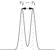
Figure 1: Two partially overlapping Gaussian pulses, separated by a time delay $\tau_{2}-\tau_{1}$.

When two photons enter a 2-channel interferometer and exactly overlap, the probability of detecting the two photons in different detectors is given the modulus squared of the permanent of the matrix $U$ describing the linear interferometer. The specific choice of a 50/50 beam splitter leads to no probability of getting one photon in each detector, as demonstrated in spectacular fashion by Hong, Ou, and Mandel [6].

The appearance of the modulus squared of a permanent is a generic feature of coincidence rates for fully indistinguishable bosons (for fermions, a determinant would replace the permanent) [7, 8, 9], and the computational complexity of this permanent is at the core of the BosonSampling paradigm, where a dilute collection of $n$ non-interacting bosons scatter inside an $m$-channel optical network with $m\gg n$.

Our results show that certain sums of rates - i.e. sums of moduli squared of immanants - computed with the original scattering matrix $U$ are equal to the same sums if $U$ is replaced by a simpler coset matrix $\bar{U}$ containing strategically placed zeroes. The number of zeroes and their placement depends in general on type of sums.

We show explicitly for $n=3$ and $n=4$ there exists a sum that has the same value if $U$ is replaced by a coset matrix $\bar{U}$ of the Hessenberg type, a special kind of “almost upper (or lower) triangular” matrix where $\bar{U}_{k,k+m}=0$ for $m=2,\ldots n-k$. The permanent of a Hessenberg matrix is actually the determinant of $T(\bar{U})$, where $T(\bar{U})$ is obtained from $\bar{U}$ by replacing $U_{k,k+1}$ by $-U_{k,k+1}$ [10]. As a result, the complexity of certain sums of rates is considerably simplified: general permanents evaluate by Ryser’s algorithm in $\mathcal{O}(2^{n-1}n^{2})$ operations whereas determinants efficiently evaluate in $\mathcal{O}(n^{3})$ operations; this is exemplified in Eq. (94), where we give the sum of rates for three indistinguishable photons. Moreover, some of the rates needed in the sums may contains multiple photon counts per channel. Thus, the submatrix required to compute the rate have rank less than $n$. In some cases, one can revert to algorithms that allow for faster permanent computation [11] of low rank matrices. We also discuss how this is generalizable to any $n$.

When particles are partially distinguishable, the rates are expressed as a sum of moduli squared of immanants [12, 2, 3, 13, 14]. In the simple case of two partially distinguishable photons, the sum contains terms proportional to (modulus squared of the) permanent and the determinant of the scattering matrix, these being special types of immanants. For the more interesting case of three input photons, one requires immanants of $3\times 3$ matrices: they are discussed in A.

Immanants of Hessenberg matrices can also be simplified as an easy corollary of results given by [10]: the computational complexity of some immanants are also in the complexity class #$\mathbb{P}$ [15, 16, 17, 18], but the immanant of a Hessenberg matrix $\bar{U}$, associated with partition of shape $\{\lambda\}$, can be computed instead using the immanant associated with the conjugate shape $\{\lambda^{*}\}$ of a transformed Hessenberg matrix $T(\bar{U})$. Thus certain sums of rates for three or more partially distinguishable photons are also simplified since we can choose to compute the simpler of the $\{\lambda\}$ or $\{\lambda^{*}\}$ immanants, although of course the savings are limited when $n$ is small. Ref. [16] provides an algorithm to evaluate the $\{\lambda\}$-immanant of an $n\times n$ matrix that has non-scalar complexity $\mathcal{O}(n^{2}s_{\lambda}d_{\lambda})$, where $s_{\lambda}$ is the number standard tableaux of shape $\lambda$ and $d_{\lambda}$ is the number of semi-standard tableaux. An immanant and its conjugate will have $s_{\lambda}=s_{\lambda^{*}}$, so to determine which of the two immanants is harder to compute, we need to look at $d_{\lambda}$ and $d_{\lambda^{*}}$. In general, the partition with the fewer number of parts will have the greater number of semi-standard tableaux, and will thus be harder to compute. For example, the immanant corresponding to $\Yboxdim{5pt}\yng(4,1)$ is more computationally expensive than its conjugate $\Yboxdim{5pt}\yng(2,1,1,1)$.

We provide here these simplifications for setups where $2$ photons interfere inside a 3-channel device, and where $3$ photons interfere inside a $4$-channel device. We explain how the simplified matrix $\bar{U}$ can be realized by removing elements in a unitary optical network. We also outline for the case of $n-1$ indistinguishable photons entering a $n\times n$ network and the corresponding savings.

2 $2$ photons in a $3$-channel interferometer

In this section we introduce the simplest case where savings by sum rules can be achieved: $2$ photons in a $3$-channel interferometer.

2.1 Connection with permanents and determinants

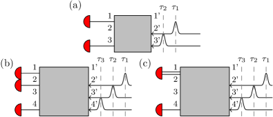
Figure 3: a) Example of a process involved in the detection of two photons entering in ports $2$ and $3$. Input photons in modes $2$ and $3$ are counted in detectors $1$, and $3$. Bottom. Examples of processes entering in the detection of three photons entering in ports $2,3$ and $4$. b) input photons in modes $2,3,4$ are counted in detectors $1$, $2$ and $4$. c) input photons in modes $2,3,4$ are counted in detectors $1$ (2 counts) and in detector 4.

The coincidence rate for two partially distinguishable photons entering in ports $2^{\prime}$ and $3^{\prime}$ of a $3$-port interferometer, see Fig. (3a), and detected in ports $1$ and $3$, is given by

$$R(23\to 13;\tau_{12}) =e^{-\tau_{12}^{2}}\left(U_{12}^{\dagger}U_{33}^{\dagger}U_{32}U_{13}+U_{12}U_{33}U_{32}^{\dagger}U_{13}^{\dagger}\right)$$

$$\quad+|U_{12}U_{33}|^{2}+|U_{13}U_{32}|^{2}\,,$$ (1)

$$=\textstyle{\frac{1}{2}}(1+e^{-\tau_{12}^{2}})|\hbox{Per}(U_{23\to 13})|^{2}$$

$$\quad+\textstyle{\frac{1}{2}}(1-e^{-\tau_{12}^{2}})|\hbox{Det}(U_{23\to 13})|^{2}\,.$$ (2)

with $\tau_{12}=\tau_{1}-\tau_{2}$. An example of this type of calculation, including the modelling of the detectors, is given in B.

When the pulses exactly overlap, i.e. when $\tau_{2}=\tau_{1}$, the rate collapses to the modulus squared of the permanent of the submatrix $U_{23\to 13}$, obtained from the original $3\times 3$ unitary matrix $U$ by keeping rows $1,3$ and columns $2,3$:

$$U=\left(\begin{array}[]{ccc}U_{11}&U_{12}&U_{13}\\ U_{21}&U_{22}&U_{23}\\ U_{31}&U_{32}&U_{33}\end{array}\right)\,,\quad U_{23\to 13}=\left(\begin{array}[]{cc}U_{12}&U_{13}\\ U_{32}&U_{33}\end{array}\right)\,.$$ (8)

If the group elements $P_{\sigma}$ of $S_{2}$ are $\{\mathds{1},P_{13}\}$, and the action of $P_{\sigma}$ is defined by the permutation of columns in the polynomial $U_{i2}U_{j3}$ so that $P_{\sigma}U_{i2}U_{j3}=U_{\sigma(i)2}U_{\sigma(j)3}$ then

$$\hbox{Per}(U_{23\to 13}) =\left(\mathds{1}+P_{13}\right)U_{12}U_{33}=U_{12}U_{33}+U_{32}U_{13}\,,$$ (9)

$$\hbox{Det}(U_{23\to 13}) =\left(\mathds{1}-P_{13}\right)U_{12}U_{33}=U_{12}U_{33}-U_{32}U_{13}\,.$$ (10)

Note that, by construction,

$$P_{13}\hbox{Per}(U_{23\to 13}) =+\hbox{Per}(U_{23\to 13})\,,$$ (11)

$$P_{13}\hbox{Det}(U_{23\to 13}) =-\hbox{Det}(U_{23\to 13})\,.$$ (12)

The permanent and the determinant examples of immanants, which are polynomial functions in the entries of a matrix, constructed here using the representations of the permutation group $S_{2}$ for two photons. These two immanants come back to multiple of themselves under any permutation or rows or columns ($+1$ for permanents, $-1$ for determinants).

2.2 Summing over the outputs

Suppose that, in addition to detecting photons in output ports $1$ and $3$ as previously described, we also count output photons at ports $2$ and $3$. We obtain the rates for this process by copying Eq. (2) with simple adjustment of the appropriate indices:

$$R(23\to 23;\tau_{12}) ={\textstyle\frac{1}{2}}(1+e^{-\tau_{12}^{2}})|\hbox{Per}(U_{23\to 23})|^{2}$$

$$\quad+{\textstyle\frac{1}{2}}(1-e^{-\tau_{12}^{2}})|\hbox{Det}(U_{23\to 23})|^{2}\,.$$ (13)

We now sum $R(23\to 23;\tau_{12})+R(23\to 13;\tau_{12})$:

$$\sum_{p=1,2}R(23\to p3;\tau_{12})={\textstyle\frac{1}{2}}(1+e^{-\frac{1}{2}\tau_{12}^{2}})\sum_{p=1,2}|\hbox{Per}(U_{23\to p3})|^{2}$$

$$\qquad\qquad+{\textstyle\frac{1}{2}}(1-e^{-\frac{1}{2}\tau_{12}^{2}})\sum_{p=1,2}|\hbox{Det}(U_{23\to p3})|^{2}$$ (14)

.

To highlight the (here elementary) simplification that occurs for this sum, we write the $3\times 3$ scattering matrix $U$ in the form of a product [19, 20], see Fig. (2b)

$$U ={\cal R}_{12}(\alpha_{1},\beta_{1},\gamma_{1})\cdot\bar{U}\,,$$ (15)

$$=\left(\begin{array}[]{ccc}e^{-i\frac{1}{2}(\alpha_{1}+\gamma_{1})}\cos\left(\frac{\beta_{1}}{2}\right)&-e^{-i\frac{1}{2}(\alpha_{1}-\gamma_{1})}\sin\left(\frac{\beta_{1}}{2}\right)&0\\ e^{-i\frac{1}{2}(\gamma_{1}-\alpha_{1})}\sin\left(\frac{\beta_{1}}{2}\right)&e^{i\frac{1}{2}(\alpha_{1}+\gamma_{1})}\cos\left(\frac{\beta_{1}}{2}\right)&0\\ 0&0&1\\ \end{array}\right)$$ (19)

$$\qquad\cdot\left(\begin{array}[]{ccc}\bar{U}_{11}&\bar{U}_{12}&0\\ \bar{U}_{21}&\bar{U}_{22}&\bar{U}_{23}\\ \bar{U}_{31}&\bar{U}_{32}&\bar{U}_{33}\end{array}\right)\,,$$ (23)

where the unitary transformation ${\cal R}_{12}(\alpha_{1},\beta_{1},\gamma_{1})$ is an $\mathrm{SU}(2)$ transformation mixing the first and second channels. Other factorizations into $\mathrm{SU}(2)$ or $\mathrm{U}(2)$ blocks are possible [21, 22, 23, 24] , but do not produce the easily identifiable coset structure required for the general $n\times n$ submatrix. The algorithms of [25] or [26] can also be used to efficiently obtain a suitable coset factorization.

One can then easily verify, using the factorized form of $U$, that the first two rows of $U$ are made to depend explicitly on the parameters $\alpha_{1},\beta_{1},\gamma_{1}$ so that each of $|\hbox{Per}(U_{23\to 23})|^{2}$, $|\hbox{Det}(U_{23\to 23})|^{2}$, $|\hbox{Per}(U_{23\to 13})|^{2}$ and $|\hbox{Det}(U_{23\to 13})|^{2}$ individually depends on these parameters. However, the sums

$$|\hbox{Per}(U_{23\to 23})|^{2}+|\hbox{Per}(U_{23\to 13})|^{2}\,,$$ (24)

and $$|\hbox{Det}(U_{23\to 23})|^{2}+|\hbox{Det}(U_{23\to 13})|^{2}$$ (25)

are actually independent of $\alpha_{1},\beta_{1},\gamma_{1}$. We denote this independence using the coset notation $\mathrm{SU}(2)\backslash U$, and refer to $\bar{U}$ as a coset matrix. We will show in detail the origin of this independence in Sec. 4.

We are therefore free to choose $\alpha_{1},\beta_{1},\gamma_{1}$ as we please: the simplest choice is to make ${\cal R}_{12}$ the unit matrix with $\alpha_{1}=\beta_{1}=\gamma_{1}=0$, so that we have an example of the core result of this Letter:

$$\sum_{p=1,2}|\hbox{Per}(U_{23\to p3})|^{2} =\sum_{p=1,2}|\hbox{Per}(\bar{U}_{23\to p3})|^{2}\,,$$ (26)

$$\sum_{p=1,2}|\hbox{Det}(U_{23\to p3})|^{2} =\sum_{p=1,2}|\hbox{Det}(\bar{U}_{23\to p3})|^{2}\,.$$ (27)

In particular we note that both

$$\hbox{Per}(U_{23\to 13}) =\hbox{Per}\left(\begin{array}[]{cc}\bar{U}_{12}&0\\ \bar{U}_{32}&\bar{U}_{33}\end{array}\right)$$ (30)

$$\hbox{Det}(U_{23\to 13}) =\hbox{Det}\left(\begin{array}[]{cc}\bar{U}_{12}&0\\ \bar{U}_{32}&\bar{U}_{33}\end{array}\right)$$ (33)

trivially evaluate to $\bar{U}_{12}\bar{U}_{33}$.

Another choice is $\alpha_{1}=\gamma_{1}=0$ but $\beta_{1}=\pi$ so the $\mathcal{R}_{12}$ matrix takes the form

$${\cal R}_{12}(0,\pi,0)=\left(\begin{array}[]{ccc}0&1&0\\ -1&0&0\\ 0&0&1\end{array}\right)$$ (37)

which yields

$${\cal R}_{12}(0,\pi,0)\bar{U}=\left(\begin{array}[]{ccc}-\bar{U}_{21}&-\bar{U}_{22}&-\bar{U}_{23}\\ \bar{U}_{12}&\bar{U}_{22}&0\\ \bar{U}_{13}&\bar{U}_{23}&\bar{U}_{33}\end{array}\right)\,,$$ (41)

showing that the results are essentially unchanged if the $0$ appears in on the second row of the last column.

If we now assume $U$ is unitary and, without loss of generality, with determinant $+1$, the resulting $U$ is an $\hbox{SU}(3)$ transformation. We can then realize the $\hbox{SU}(3)$ transformation describing the inteferometer as a sequence of $\hbox{SU}(2)$ inteferometers mixing modes $(12)$, $(23)$ and then $(12)$ again [20]:

$$U={\cal R}_{12}(\alpha_{1},\beta_{1},\gamma_{1}){\cal R}_{23}(\alpha_{2},\beta_{2},\alpha_{2}){\cal R}_{12}(\alpha_{3},\beta_{3},\gamma_{3})\,.$$ (42)

Summing the rates for $U$ then yields the same result as summing the rates over a scattering matrix $\bar{U}$ describing an inteferometer with the rightmost element removed, as illustrated in Fig. (2b).

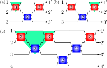
Figure 2: The numbers in each box represents the number of parameters in the corresponding $\hbox{SU}(2)$ transformation. Numbers at the sides label port number. Input ports are on the right. a) Diagrammatic form of the decomposition of an $\hbox{SU}(3)$ matrix as a sequence of $\hbox{SU}(2)$ matrices. The numbers in the boxes are the numbers of independent angles in each $\hbox{SU}(2)$ transformation. When the rates at output channels $(p3)$ are summed over $p=1,2$, the $\hbox{SU}(2)$ transformation highlighted in green, ${\cal R}_{12}(\alpha_{3},\beta_{3},\gamma_{3})$, can be replaced by the unit matrix, or the equivalent optical element can be removed, yielding a coset transformation $\hbox{SU}(2)\backslash\hbox{SU}(3)$. See Eq. (42). b) When rates at input channels $(p3)$ are summed over $p=1,2$, the $\hbox{SU}(2)$ transformation highlighted in green, ${\cal R}_{12}(\alpha_{1},\beta_{1},\gamma_{1})$, can be replaced by the unit matrix, or the equivalent optical element can be removed, yielding a coset transformation $\hbox{SU}(3)/\hbox{SU}(2)$. See Eq. (42). c) Diagrammatic representation of a $\hbox{SU}(4)$ matrix decomposed in $\hbox{SU}(2)$ transformations. Green triangle highlights the $\hbox{SU}(3)$ submatrix, ${\cal R}_{123}$, see Eq. (75).

2.3 Symmetry analysis

One can understand the origin of the independence on the $\hbox{SU}(2)$ parameters $\alpha_{1},\beta_{1},\gamma_{1}$ as follows. Define

$$\hat{A}^{\dagger}_{k}(\tau_{m}) \equiv\int d\mu\,e^{i\mu\tau_{m}}\phi(\mu)\hat{a}_{k}^{\dagger}(\mu)\,,$$ (43)

$$\hat{C}_{ij} =A_{i}^{\dagger}(\tau_{1})\hat{A}_{j}(\tau_{1})+\hat{A}_{i}^{\dagger}(\tau_{3})\hat{A}_{j}(\tau_{3})\,,$$ (44)

where $\phi(\mu)$ is the spectral profile of a pulse in channel $k$, and construct the $\mathfrak{su}(2)$ subalgebra

$$\hat{C}_{12} \mapsto\hat{L}_{+}\,,\qquad\hat{C}_{21}\mapsto\hat{L}_{-}\,,\quad\hat{C}_{11}-\hat{C}_{22}\mapsto 2\hat{L}_{z}\,.$$ (45)

One can easily verify that 2-photon output states of the type

$$|\psi_{13}\rangle_{+} =\left(\hat{A}^{\dagger}_{1}(\tau_{1})\hat{A}_{3}^{\dagger}(\tau_{3})+\hat{A}^{\dagger}_{1}(\tau_{3})\hat{A}_{3}^{\dagger}(\tau_{1})\right)|0\rangle\,,$$ (46)

$$|\psi_{13}\rangle_{-} =\left(\hat{A}^{\dagger}_{1}(\tau_{1})\hat{A}_{3}^{\dagger}(\tau_{3})-\hat{A}^{\dagger}_{1}(\tau_{3})\hat{A}_{3}^{\dagger}(\tau_{1})\right)|0\rangle$$ (47)

are killed by $\hat{C}_{12}$ so the sets $\{|\psi_{13}\rangle_{\pm},\hat{C}_{21}|\psi_{13}\rangle_{\pm}\}_{\pm}$ each span a 2-dimensional representation of this $\mathfrak{su}(2)$. (Note that, when $\tau_{3}=\tau_{1}$, only the states $|\psi_{13}\rangle_{+}$ and $\hat{C}_{21}|\psi_{13}\rangle_{+}$ survive.)

Therefore, by summing over detected states of the type $\hat{A}^{\dagger}_{1}(\tau_{i})\hat{A}_{3}^{\dagger}(\tau_{j})|0\rangle$ and $\hat{A}^{\dagger}_{2}(\tau_{i})\hat{A}_{3}^{\dagger}(\tau_{j})|0\rangle$, we are summing over complete sets of $\mathfrak{su}(2)$ states, eliminating the dependence on the matrix ${\cal R}_{12}(\alpha_{1},\beta_{1},\gamma_{1})$.

2.4 Summing over the inputs

A similar conclusion is reached —assuming both input configurations with equal time delays, v.g., $\tau_{2}-\tau_{3}=\tau_{1}-\tau_{3}$ if we fix the output to ports $2,3$ but now sum over the input channels $1,3$ and $2,3$. In this case, the rates are computed using submatrices of the type

$${U}_{p3\to 23}=\begin{pmatrix}{U}_{2p}&{U}_{23}\\ {U}_{3p}&{U}_{33}\end{pmatrix}\,,\qquad p=1,2\,.$$ (48)

We now factorize the scattering matrix $U$ as the product

$$U =\tilde{U}\cdot{\cal R}_{12}(\alpha_{3},\beta_{3},\gamma_{3})\,,$$ (49)

$$=\left(\begin{array}[]{ccc}\tilde{U}_{11}&\tilde{U}_{12}&\tilde{U}_{13}\\ \tilde{U}_{21}&\tilde{U}_{22}&\tilde{U}_{23}\\ 0&\tilde{U}_{32}&\tilde{U}_{33}\end{array}\right)$$ (53)

$$\quad\cdot\left(\begin{array}[]{ccc}e^{-\frac{i}{2}(\alpha_{3}+\gamma_{3})}\cos\left(\frac{\beta_{3}}{2}\right)&-e^{-\frac{i}{2}(\alpha_{3}-\gamma_{3})}\sin\left(\frac{\beta_{3}}{2}\right)&0\\ e^{-\frac{i}{2}(\gamma_{3}-\alpha_{3})}\sin\left(\frac{\beta_{3}}{2}\right)&e^{\frac{i}{2}(\alpha_{3}+\gamma_{3})}\cos\left(\frac{q_{3}}{2}\right)&0\\ 0&0&1\\ \end{array}\right)\,,$$ (57)

as illustrated in Fig. (2a). Summing the rates over inputs $1,3$ and $2,3$, we find the sum does not depend on $\alpha_{3},\beta_{3},\gamma_{3}$, so we can choose ${\cal R}_{12}$ to be the unit matrix and use $\tilde{U}$, with the leftmost element removed, as illustrated in Fig. (2a).

3 $3$ photons in a $4$-channel interferometer: $\hbox{SU}(3)\backslash U$

In this section we discuss the savings resulting from sum rules corresponding to the extension of the previous case: $3$ photons in a $4$-channel interferometer. We present this case because it illustrates all the features present in configurations with more than $2$ photons.

3.1 Summing over outputs

We consider without loss of generality the situation when $3$ photons access to the interferometer by channels $1^{\prime}$, $2^{\prime}$, and $4^{\prime}$, while detectors are put at output channels $2$, $3$ and $4$. We will sum over processes where one of the three photons is always counted in channel $4$.

First, suppose photons are counted one each in detectors $1,2$ and $4$, as in Fig. (3b). Computation of the rates now involves immanants of the $3\times 3$ submatrix

$$U_{234\to 124}=\left(\begin{array}[]{ccc}U_{12}&U_{13}&U_{14}\\ U_{22}&U_{23}&U_{24}\\ U_{42}&U_{43}&U_{44}\end{array}\right)\,$$ (61)

obtained by keeping columns $2,3,4$ and rows $1,2,4$. Similarly if photons are counted in detectors $1,3,4$ we keep now rows $1,3,4$, and if they are counted one each in detectors $2,3,4$ we keep rows $2,3,4$ of the submatrix.

If one photon is counted in detector $4$ but two are counted in detector $2$, we need to duplicate row $2$ in the submatrix:

$$U_{234\to 224}=\left(\begin{array}[]{ccc}U_{22}&U_{23}&U_{24}\\ U_{22}&U_{23}&U_{24}\\ U_{42}&U_{43}&U_{44}\end{array}\right)\,,$$ (65)

and similarly appropriately duplicate rows when two photons are counted in detector $3$ and one in detector $4$, and two are counted in detector $2$ and one in detector $4$. This feature of summing rates with multiple photons in one port is not present in the first case Sec. 2, and also not present in BosonSampling, where the probability of having multiple photons in a single output detector is kept low by diluting $n\ll m$.

If we now sum the rates associated with this input setup we find, irrespective of the relative input delays , that the sums are all identical to those obtained by using the appropriate submatrices of the simpler matrix

$$\bar{U}=\left(\begin{array}[]{cccc}\bar{U}_{11}&\bar{U}_{12}&0&0\\ \bar{U}_{21}&\bar{U}_{22}&\bar{U}_{23}&0\\ \bar{U}_{31}&\bar{U}_{32}&\bar{U}_{33}&\bar{U}_{34}\\ \bar{U}_{41}&\bar{U}_{42}&\bar{U}_{43}&\bar{U}_{44}\end{array}\right)\,.$$ (70)

In other words, we write the full scattering matrix

$$U={\cal R}_{123}\cdot\bar{U}\,,\quad{\cal R}_{123}=\left(\begin{array}[]{cccc}*&*&*&0\\ &*&*&0\\ &*&*&0\\ 0&0&0&1\end{array}\right)$$ (75)

with ${\cal R}_{123}$ an SU$(3)$ matrix, depending on $8$ parameters, mixing only modes $1$, $2$ and $3$. With this factorization one shows that the sum of rates is independent of the $8$ parameters of ${\cal R}_{123}$.

Assuming the transformation $U$ is unitary with determinant $+1$, we can realize this transformation as an SU$(4)$ interferometer decomposed in a sequence of $\hbox{SU}(2)$ transformations as in [20]. The independence of the sum on the $8$ parameters of ${\cal R}_{123}$ is equivalent to removing three optical elements in the system, as illustrated in Fig. (2c).

From Eq. (70) it follows that the submatrices of $\bar{U}$ are of the form

$$\bar{U}_{234\to 124}=\left(\begin{array}[]{ccc}\bar{U}_{12}&0&0\\ \bar{U}_{22}&\bar{U}_{23}&0\\ \bar{U}_{42}&\bar{U}_{43}&\bar{U}_{44}\end{array}\right)\,.$$ (79)

Two other examples of submatrices needed are

$$\bar{U}_{234\to 134} =\left(\begin{array}[]{ccc}\bar{U}_{12}&\bar{U}_{13}&0\\ \bar{U}_{32}&\bar{U}_{33}&\bar{U}_{34}\\ \bar{U}_{42}&\bar{U}_{43}&\bar{U}_{44}\end{array}\right)\,,$$ (83)

$$\bar{U}_{234\to 224} =\left(\begin{array}[]{ccc}\bar{U}_{22}&\bar{U}_{23}&0\\ \bar{U}_{22}&\bar{U}_{23}&0\\ \bar{U}_{42}&\bar{U}_{43}&\bar{U}_{44}\end{array}\right)\,.$$ (87)

The matrix $\bar{U}$ and the submatrices of (79), (83) and (87) are of the Hessenberg type, i.e. matrices where $\bar{U}_{i,i+k}=0$ for $k\geq 2$. These have the following important property: the computation of the permanent of such matrices can be mapped to the computation of the determinant of a matrix $T(U)$, obtained from $U$ by changing the entries $U_{i,i+1}$ to their negatives [10]. In other words, we have for instance

$$\hbox{Per}(\bar{U}_{234\to 134}) =\hbox{Det}(T(\bar{U})_{234\to 134})\,,$$ (88)

$$T(\bar{U})_{234\to 134} =\left(\begin{array}[]{ccc}\bar{U}_{12}&-\bar{U}_{13}&0\\ \bar{U}_{32}&\bar{U}_{33}&-\bar{U}_{34}\\ \bar{U}_{42}&\bar{U}_{43}&\bar{U}_{44}\end{array}\right)\,,$$ (92)

and similarly for the other matrices of the Hessenberg type. In particular, the matrix $\bar{U}_{234\to 124}$ is triangular so we have $\hbox{Per}(\bar{U}_{234\to 123})=\hbox{Det}(\bar{U}_{234\to 123})=\bar{U}_{12}\bar{U}_{23}\bar{U}_{44}$.

Thus, for instance, if all three photons are coincident at input, the sum of output rates is a sum of permanents of submatrices:

$$\sum_{p=1}^{2}\sum_{q=p+1}^{3}|\hbox{Per}(U_{234\to pq4})|^{2}+{\textstyle\frac{1}{2}}\sum_{p=1}^{3}|\hbox{Per}(U_{234\to pp4})|^{2}$$

$$=\sum_{p=1}^{2}\sum_{q=p+1}^{3}|\hbox{Per}(\bar{U}_{234\to pq4})|^{2}+{\textstyle\frac{1}{2}}\sum_{p=1}^{3}|\hbox{Per}(\bar{U}_{234\to pp4})|^{2}\,,$$ (93)

$$=\sum_{p=1}^{2}\sum_{q=p+1}^{3}|\hbox{Det}(T(\bar{U})_{234\to pq4})|^{2}+{\textstyle\frac{1}{2}}\sum_{p=1}^{3}|\hbox{Per}(\bar{U}_{234\to pp4})|^{2}\,,$$ (94)

Note that an extra factor $\frac{1}{2}$ multiplies those terms describing the detection of two identical photons in the same detector since a state containing two identical particles has an extra $\sqrt{2!}$ denominator factor for proper normalization. The origin of this extra factor is discussed at some greater length in Sec. 4.

3.2 Partially indistinguishable wave packets and Immanants

Although more complicated to generalize, the situation is more interesting when not all three photons exactly overlap. There are now three possible types of rates, associated with the three possible Young diagrams labelling the irreps of $S_{3}$. They are $\Yboxdim{5pt}\yng(3)$, $\Yboxdim{5pt}\yng(1,1,1)$ and $\Yboxdim{5pt}\yng(2,1)$. The first type corresponds to the fully symmetric representation: if the three input photons are fully indistinguishable, the coincidence rates are only a function of permanents of a $3\times 3$ submatrix. If two of the photons are indistinguishable, the rates now depend not only on the permanent of a submatrix but also on some immanants of the type $\Yboxdim{5pt}\yng(2,1)$ of this submatrix. If all three photons are partially indistinguishable, the rates also include contributions from the determinant of a $3\times 3$ matrix in addition to the previous immanants.

Immanants generalize permanents and determinants, and additional details on immanants of a $3\times 3$ matrix can be found in A.

Our formalism also requires the counting two photons in any one of the detectors. We can accommodate this by using a $3\times 3$ submatrix constructed from the full scattering matrix by duplicating the appropriate column or row of $U$. The immanants of this submatrix are then computed in the usual way (of course in this case any determinant is automatically $0$).

We discuss here the case where $\tau_{1}=\tau_{2}\neq\tau_{3}$, and we assume for simplicity that $U$ is unitary with determinant $+1$. In this case the 3-photon input states belong to the irreps $(3,0,0)$ (or $\Yboxdim{5pt}\yng(3)$) of $\hbox{SU}(4)$, or to the irrep $(1,1,0)$ (or $\Yboxdim{5pt}\yng(2,1)$) of $\hbox{SU}(4)$. Rates are no longer given by the permanent of a submatrix, but must also include immanants associated with $\Yboxdim{5pt}\yng(2,1)$ partition of the permutation group $S_{3}$ of the three photons, see Eq. (131).

For instance:

$$R(234\to pp4;\tau_{13})={\textstyle\frac{1}{3}}(1+2e^{-\tau_{13}^{2}})|\operatorname{\mathrm{Per}}(U_{234\to pp4})|^{2}$$

$$+{\textstyle\frac{2}{3}}(1-e^{-\tau_{13}^{2}})|\mathrm{Imm}^{\Yboxdim{5pt}\yng(2,1)}(U_{234\to pp4})|^{2}\,,$$ (95)

$$R(234\to pq4;\tau_{13})=|\mathcal{A}|^{2}+|\mathcal{B}|^{2}+|\mathcal{C}|^{2}$$

$$+e^{-\tau_{13}^{2}}\left[(\mathcal{A}+\mathcal{B})^{*}\mathcal{C}+(\mathcal{B}+\mathcal{C})^{*}+(\mathcal{C}+\mathcal{A})^{*}\mathcal{B}\right],$$ (96)

where the functions $\mathcal{A}$, $\mathcal{B}$, and $\mathcal{C}$ are related to immanants by

$$\mathcal{A} ={\textstyle\frac{1}{3}}(\operatorname{\mathrm{Per}}(U_{234\to pq4})-\mathrm{Imm}^{\Yboxdim{5pt}\yng(2,1)}(U_{243\to pq4})$$

$$\qquad-\mathrm{Imm}^{\Yboxdim{5pt}\yng(2,1)}(U_{324\to pq4})+\mathrm{Imm}^{\Yboxdim{5pt}\yng(2,1)}(U_{342\to pq4})),$$ (97)

$$\mathcal{B} ={\textstyle\frac{1}{3}}(\operatorname{\mathrm{Per}}(U_{234\to pq4})-\mathrm{Imm}^{\Yboxdim{5pt}\yng(2,1)}(U_{234\to pq4})$$

$$\quad+\mathrm{Imm}^{\Yboxdim{5pt}\yng(2,1)}(U_{243\to pq4})-\mathrm{Imm}^{\Yboxdim{5pt}\yng(2,1)}(U_{324\to pq4})$$

$$\quad-\mathrm{Imm}^{\Yboxdim{5pt}\yng(2,1)}(U_{342\to pq4})),$$ (98)

$$\mathcal{C} ={\textstyle\frac{1}{3}}(\operatorname{\mathrm{Per}}(U_{234\to pq4})+\mathrm{Imm}^{\Yboxdim{5pt}\yng(2,1)}(U_{234\to pq4}))$$

$$\quad+\mathrm{Imm}^{\Yboxdim{5pt}\yng(2,1)}(U_{324\to pq4})),$$ (99)

with $\tau_{13}=\tau_{1}-\tau_{3}$. The notation $\mathrm{Imm}^{\Yboxdim{5pt}\yng(2,1)}(U_{ijk\to pq4})$ indicates that the immanant is calculated using the matrix $U_{ijk\to pq4}$ where the columns of $U_{234\to pq4}$ are permuted to the order $ijk$. Both Eqs.(95) and (96) correctly collapse to a single permanent when $\tau_{13}=0$.

With the appearances of immanants, one can ask if simplifications similar to those of Eq. (94) occur. Indeed one can show that the immanant $\hbox{Imm}^{\{\lambda\}}(\bar{U})$ of a Hessenberg matrix $\bar{U}$ maps to the calculation of the immanant $\hbox{Imm}^{\{\lambda\}^{*}}(T(\bar{U}))$ where $\{\lambda\}^{*}$ is the partition conjugate to $\{\lambda\}$. In the specific case of immanants of the type $\Yboxdim{7pt}\yng(2,1)$ needed for our $3$-photon problem, there is no associated savings as the partition $\Yboxdim{7pt}\yng(2,1)$ is self-conjugate.

4 $n-1$ photons in a $n$-channel interferometer

In this section we discuss the mathematical origin of the simplifications in sums presented in previous sections, Eqs. (26), (27), and (94). First, we reconsider the case in Sec. 2 in terms of group functions  [9, 27]. We then proceed to extend the result for $n$ indistinguishable photons. In this section we assume that the transformation $U$ is unitary.

4.1 $2$ photons in a $3$-channel interferometer in terms of group functions

Irreducible representations of the unitary groups, like irreducible representations of the permutation group, are also labelled by Young diagrams [28]. In this notation, a single photon state in a $3$-channel interferometer will transform by representation $(1,0)$ of $\mathrm{SU}(3)$, whereas two-photon states will transform by the representation $(1,0)\otimes(1,0)$. This representation is reducible, and the reduction [29, 30] indeed often uses Young diagrams as a convenient calculational device [28, 31] :

$$\begin{array}[]{ccccccc}(1,0)&\otimes&(1,0)&=&(2,0)&\oplus&(0,1)\\ \Yboxdim{7pt}\yng(1)&\otimes&\Yboxdim{7pt}\yng(1)&=&\Yboxdim{7pt}\yng(2)&\oplus&\Yboxdim{7pt}\yng(1,1)\end{array}\,.$$ (102)

The $\hbox{SU}(3)$ irrep $(a,b)$ has dimension $\frac{1}{2}(a+1)(b+1)(a+b+2)$. The representation $(2,0)$ or $\Yboxdim{7pt}\yng(2)$ is therefore $6$-dimensional; it contains the symmetric states $\{|100\rangle|100\rangle$,$\frac{1}{\sqrt{2}}\bigl{(}|100\rangle|010\rangle$+ $|010\rangle|100\rangle\bigr{)}\ldots\}$, immediately generalizing to $\hbox{SU}(3)$ the well known spin-triplet states. The $3$-dimensional representation $(0,1)$ or $\Yboxdim{7pt}\yng(1,1)$ contains the antisymmetric states $\{\frac{1}{\sqrt{2}}\left(|100\rangle|010\rangle-|010\rangle|100\rangle\right)\ldots\}$, again generalizing to $\hbox{SU}(3)$ the well-known antisymmetric $\hbox{SU}(2)$ singlet.

Immanants are quite generally related to group functions [32]:

$$\hbox{Per}\left(\begin{array}[]{cc}U_{2p}&U_{23}\\ U_{3p}&U_{33}\end{array}\right)=D^{\Yboxdim{5pt}\yng(2)}_{(23);(p3)}(U)\,,$$ (105)

$$\hbox{Det}\left(\begin{array}[]{cc}U_{2p}&U_{23}\\ U_{3p}&U_{33}\end{array}\right)=D^{\Yboxdim{5pt}\yng(1,1)}_{(23);(p3)}(U)\,,$$ (108)

where $(p3)$ denotes a state where photons enter in input channel $p=1,2$ and in channel $3$, so that for instance $(13)$ for photons entering in input channels $1$ and $3$.

In this notation, we therefore have, for the summation over the inputs with fixed output channels,

$$\sum_{p=1,2}|D^{\Yboxdim{5pt}\yng(2)}_{(23);(p3)}(U)|^{2}=\sum_{p=1,2}|D^{\Yboxdim{5pt}\yng(2)}_{(23);(p3)}(\bar{U})|^{2}\,,$$ (109)

$$\sum_{p=1,2}|D^{\Yboxdim{5pt}\yng(1,1)}_{(23);(p3)}(U)|^{2}=\sum_{p=1,2}|D^{\Yboxdim{5pt}\yng(1,1)}_{(23);(p3)}(\bar{U})|^{2}$$ (110)

where the $(13)$ and $(23)$ states span an $\hbox{SU}(2)$ subrepresentation of $\hbox{SU}(3)$ inside the $\Yboxdim{7pt}\yng(2)$ representation, and a subrepresentation of $\hbox{SU}(3)$ in the $\Yboxdim{7pt}\yng(1,1)$ representation.

The corresponding sums over outputs with fixed inputs are simply

$$\sum_{p=1,2}|D^{\Yboxdim{5pt}\yng(2)}_{(p3);(23)}(U)|^{2}=\sum_{p=1,2}|D^{\Yboxdim{5pt}\yng(2)}_{(p3);(23)}(\bar{U})|^{2}\,,$$ (111)

$$\sum_{p=1,2}|D^{\Yboxdim{5pt}\yng(1,1)}_{(p3);(23)}(U)|^{2}=\sum_{p=1,2}|D^{\Yboxdim{5pt}\yng(1,1)}_{(p3);(23)}(\bar{U})|^{2}\,.$$ (112)

We can show this explicitly for the permanent as follows. Let us denote by $|(2,0)p_{1}p_{2};I\rangle$ a basis states for the $(2,0)$ (or $\Yboxdim{5pt}\yng(2)$) irrep of $\mathfrak{su}(3)$, with $I$ the $\mathfrak{su}(2)$ label form states transforming by the irrep $I$ of the ${\cal R}_{12}$ subgroup. Here $(p_{1},p_{2})=(1,1)$ denotes two photons in mode $1$, while $(p_{1},p_{2})=(1,3)$ denote one photon in mode $1$ and one in mode $3$.

Then [32]:

$$\hbox{Per}(U_{23\to q3})=\langle(2,0)q3|U|(2,0)23\rangle$$ (113)

With this notation

$$\sum_{q=1,2}|\hbox{Per}(U_{23\to q3})|^{2}$$

$$=\sum_{q=1,2}\langle(2,0)q3|U|(2,0)23\rangle\langle(2,0)q3|U|(2,0)23\rangle^{*}\,.$$ (114)

At this point, we split the transformation $U={\cal R}_{12}(\omega_{1})\bar{U}$, with $\omega_{1}=(\alpha_{1},\beta_{1},\gamma_{1})$ parametrizing an $\mathrm{SU}(2)$ transformation:

$$\sum_{q=1,2}|\hbox{Per}(U_{23\to q3})|^{2}$$

$$=\sum_{q,\gamma,\gamma^{\prime}=1,2}\langle(2,0)q3|{\cal R}_{12}(\omega_{1})|(2,0)\gamma 3\rangle\langle(2,0)\gamma 3|\bar{U}|(2,0)23\rangle$$

$$\times\langle(2,0)q3|{\cal R}_{12}(\omega_{1})|(2,0)\gamma^{\prime}3\rangle^{*}\langle(2,0)\gamma^{\prime}3|\bar{U}|(2,0)23\rangle^{*}\,,$$ (115)

and explicitly use the $\mathrm{SU}(2)$ $D$-function for the ${\cal R}_{12}(\omega_{1})$ transformation

$$\sum_{q=1,2}|\hbox{Per}(U_{23\to q3})|^{2}=\sum_{\gamma\gamma^{\prime}}\left(\sum_{q}D^{1/2}_{\mathcal{W}(q)w(\gamma)}(\omega_{1})\left(D^{1/2}_{\mathcal{W}(q)w(\gamma^{\prime})}(\omega_{1})\right)^{*}\right)$$

$$\qquad\times\langle(2,0)\gamma 3|\bar{U}|(2,0)23\rangle^{*}\langle(2,0)\gamma^{\prime}3|\bar{U}|(2,0)23\rangle^{*}\,,$$ (116)

where

$$\mathcal{W}(q)=\left\{\begin{array}[]{cc}+\frac{1}{2}&\hbox{if }q=1;\\ -\frac{1}{2}&\hbox{if }q=2,\end{array}\right.$$ (119)

and $w(\gamma)$ likewise defined so it takes the values $\pm\frac{1}{2}$. The sums of $D$-functions with the same angle satisfy:

$$\sum_{\mathcal{W}(q)}D^{1/2}_{\mathcal{W}(q)w(\gamma)}(\omega_{1})\left(D^{1/2}_{\mathcal{W}(q)w(\gamma^{\prime})}(\omega_{1})\right)^{*}=\delta_{\gamma\gamma^{\prime}}$$ (120)

so that the sum collapses to

$$\sum_{q=1,2}|\hbox{Per}(U_{23\to q3})|^{2}$$

$$=\sum_{\gamma}\langle(2,0)\gamma 3|\bar{U}|(2,0)23\rangle\langle(2,0)\gamma 31|\bar{U}|(2,0)23\rangle^{*}\,,$$ (121)

$$=\sum_{\gamma=1,2}|\hbox{Per}(\bar{U}_{23\to\gamma 3})|^{2}\,,$$ (122)

which shows the first part of the result.

The results for the determinant follows the same steps, but with the replacement of the irrep $(2,0)$ (or $\Yboxdim{5pt}\yng(2)$) by $(0,1)$ or $(2,0)$ (or $\Yboxdim{5pt}\yng(1,1)$), and the identification

$$\hbox{Det}(U_{23\to q3})=\langle(0,1)q3|U|(0,1)23\rangle\,.$$ (123)

4.2 Generalization for $n-1$ photons in a $n$-channel interferometer

We extend the ideas presented in Sec. 4.1 to the general case of $n-1$ indistinguishable photons. We consider the following sum of rates

$$\sum_{\vec{}\eta}c_{\vec{}\eta}R(\vec{\xi}\to\vec{}\eta n),$$ (124)

where $\vec{}\eta=(\eta_{1},\eta_{2},\cdots,\eta_{n-2})$ is a vector of length $n-2$, with $\eta_{i}$ indicating a photon in mode $i$. Thus, for two photon in the first three modes of an interferometer we can have $\vec{}\eta=(1,1)$, $(1,2)$, $(1,3)$, $(2,2)$, $(2,3)$ and $(3,3)$, with $(2,2)$ indicating two photons in mode $2$. The factor $c_{\vec{}\eta}$ is the inverse of the product of factorials corresponding to the repetitions in $\vec{}\eta$. For instance, for $\vec{}\eta=(1,2,1,1,2)$, $c_{\vec{}\eta}=1/(2!3!)$. This factor arises because, if a mode contains $k$ photons, it must be normalized by dividing the state by $1/\sqrt{k!}$, and the rate by $1/k!$ since the rate is proportional to modulus square of the matrix element involving the state.

Likewise, $\vec{\xi}$ is a vector of length $(n-1)$ where $\xi_{i}$ has the same interpretation as $\eta_{i}$. To keep the discussion simple we assume that all $\xi_{i}$ are distinct $(c_{\vec{\xi}}=1)$, although this is not essential.

For $(n-1)$ indistinguishable photons, each rate $R(\vec{\xi}\to\vec{}\eta n)$ is proportional to the modulus squared for the permanent of the submatrix $U_{\vec{\xi}\to\vec{}\eta n}$, and this permanent is related to the function [9]

$$\sqrt{c_{\vec{}\eta}}\operatorname{\mathrm{Per}}(U_{\vec{\xi}\to\vec{}\eta n})=$$

$$\langle(n-1,0,\ldots,0)\vec{}\eta n|{\cal R}_{1\cdots n-1}(\omega_{1\cdots n-1})\bar{U}|(n-1,0,\ldots,0)\vec{\xi}\rangle$$ (125)

where we have again split $U$ into an $\mathrm{SU}(n-1)$ transformation and a coset transformation: $U={\cal R}_{1\cdots n-1}(\omega_{1\cdots n-1})\bar{U}$. The strategy is again to insert a complete set of $\mathrm{SU}(n-1)$ states between the subgroup and the coset transformations:

$$\langle(n-1,0,\cdots,0)\vec{}\eta n|{\cal R}_{1\cdots n-1}(\omega_{1\cdots n-1})\bar{U}|(n-1,0,\cdots,0)\vec{\xi}\rangle$$

$$=\sum_{\vec{}\rho}\langle(n-1,0,\cdots,0)\vec{}\eta n|{\cal R}_{1\cdots n-1}(\omega_{1\cdots n-1})|(n-1,0,\cdots,0)\vec{}\rho n\rangle$$

$$\quad\times\langle(n-1,0,\cdots,0)\vec{}\rho n|\bar{U}|(n-1,0,\ldots,0)\vec{\xi}\rangle\,,$$ (126)

$$=\sum_{\vec{}\rho}D^{(n-1,0,\cdots,0)}_{\vec{}\eta n;\vec{}\rho n}(\omega_{1\cdots n-1})$$

$$\quad\times\langle(n-1,0,\cdots,0)\vec{}\rho n|\bar{U}|(n-1,0,\ldots,0)\,.$$ (127)

Multiplying by the complex conjugate, summing as per Eq. (124), and using the orthogonality of the $D^{(n-1,0,\cdots,0)}_{\vec{}\eta n;\vec{}\rho n}(\omega_{123\cdots n-1})$ functions yields the result.

A similar proof can be developed for the case of partially distinguishable photons, using the connection between immanants of a submatrix of a unitary matrix and group functions.

5 Concluding remarks

In this Letter we presented a method of computing sums of coincidence rates using a coset matrix describing a simplified scattering process, resulting in reduced computational complexity compared to the original problem. The result depends on factoring the original $n\times n$ scattering matrix into an $\hbox{SU}(n-1)$ matrix and a coset matrix, and summing over states which span subrepresentations of $\hbox{SU}(n-1)$ inside our many-photon Hilbert space.

The coset matrices $\bar{U}$ discussed in this Letter are of the Hessenberg type (though not all Hessenberg matrices are coset matrices and not every submatrix of a Hessenberg matrix is Hessenberg), and additional simplifications in evaluating permanents of such matrices are possible: we show explicitly that certain sums of modulus squared of permanents of $3\times 3$ submatrices of $\hbox{SU}(4)$, can be evaluated using sums of modulus squared of determinants.

Additional simplifications in the evaluations of immanants which arise when photons are not all coincident, are also known to occur Hessenberg matrices [10], but for the specific case of $3\times 3$ submatrices of $\hbox{SU}(4)$ there is no savings since the $\Yboxdim{5pt}\yng(2,1)$ is self-conjugate.

We note that good algorithms to evaluate immanants of unitary matrices are difficult to find. Following Kostant [27] (see also [32]) Bürgisser [16] proposed to evaluate immanants using sums of group functions, a strategy that displaces the problem of constructing of such functions. In addition, the map $T$ that transforms the evaluation of the immanant of a Hessenberg matrix $\bar{U}$ to its simplified form $T(\bar{U})$ as per Eq. (92), is such that $T(\bar{U})$ is not unitary. As a result the challenge of implementing this transformation and neatly evaluating the simplified immanants by anything other than a brute force method remains an open problem at this time.

We did not discuss the case where the coset is of the type ${\cal R}\bar{U}$ with ${\cal R}\in\hbox{SU}(k)$ and $k<n-1$: the detailed analysis of the possible simplifications arising from the factorization of $\hbox{SU}(k)$ submatrices of the original $n\times n$ matrix $U$ remains at this time an open question.

When $k$ is small, the savings that result from the summations are small since few $0$s will appear in the coset matrices. When $k$ is large, the savings are more substantial, although the summations must include rates for processes where more than one photon is counted in some detectors. This suggests that one can devise a series of increasingly sophisticated tests based on sums to verify the proper functioning of the optical network. The extent to which one can construct an efficient witness based on sums of rates remains to be explored, although constructing coset matrices $\bar{U}$ from the original $U$ can be done efficiently using Householder transformations [25, 26].

6 Acknowledgements

DAA acknowledges support from projects CONACyT 285754, UNAM-PAPIIT IG100518, and from the Mitacs-CALAREO Globalink Research Award Program. Dylan Spivak acknowledges support from the Ontario Graduate Scholarship program. The work of HdG is supported by NSERC of Canada. We thank Olivia DiMatteo and Barry Sanders for comments and useful discussions.

Appendix A Immanants of $3\times 3$ matrix

Immanants are weighted sums of products of matrix entries:

$$\hbox{Imm}^{\{\lambda\}}(U)=\sum_{\sigma\in S_{n}}\chi^{\{\lambda\}}(\sigma)U_{\sigma(1)1}U_{\sigma(2)2}\ldots U_{\sigma(n)n}$$ (128)

where $\{\lambda\}$ is a partition of $n$ labelling an irreducible representation of $S_{n}$ and $\chi^{\{\lambda\}}(\sigma)$ is the character of $\sigma\in S_{n}$ for the irrep $\lambda$.

A convenient mnemonic device to label partitions and therefore irreducible representations of $S_{n}$ is to use Young diagrams, [33, 28, 34],[28]. A convenient mnemonic device to label partitions and therefore irreducible representations of $S_{n}$ is to use Young diagrams The partition $\{\lambda\}=(\lambda_{1},\lambda_{2},\ldots,\lambda_{k})$ with $\lambda_{k}\geq\lambda_{k+1}$ is pictorially represented by a left-justified diagram containing $\lambda_{k}$ boxes on row $k$. The partition $\{n\}$ of $n$, used for the permanent, corresponds to the one-rowed Young diagram $\Yboxdim{7pt}\yng(3)\cdots\yng(1)$ containing $n$ boxes on the row, while the partition $\{1^{n}\}$ used for determinants corresponds to a Young diagram with a single column of $n$ boxes.

To complete the calculation of an immanant, we need the characters of the appropriate representation. These can be computed from scratch or found elsewhere[12]. The characters of the three irreducible representations of $S_{3}$ are given in Tab. (1).

Elements	$\mathds{1}$	$\{P_{12},P_{13},P_{23}\}$	$\{P_{123},P_{132}\}$
irrep $\lambda$	$\chi^{\lambda}(\mathds{1})$	$\chi^{\lambda}(P_{ab})$18pt$\yng(1,1)$	$\chi^{\lambda}(P_{abc})$	dim.
$\Yvcentermath 1\Yboxdim{6pt}\yng(3)$	1	1	1	1
$\Yvcentermath 1\Yboxdim{6pt}\yng(2,1)$	2	0	-1	2
$\Yvcentermath 1\Yboxdim{6pt}\yng(1,1,1)$	1	-1	1	1

Table 1: The character table for $S_{3}$.

Using Tab. (1), the immanants for $3\times 3$ matrices are

$$\hbox{Imm}^{\Yboxdim{5pt}\yng(3)}(U) =\sum_{\sigma}P_{\sigma}U_{11}U_{22}U_{33}=\hbox{Per}(U)\,,$$ (129)

$$\hbox{Imm}^{\Yboxdim{5pt}\yng(1,1,1)}(U) =U_{11}U_{22}U_{33}-(P_{12}+P_{13}+P_{23})U_{11}U_{22}U_{33}$$

$$\quad+(P_{123}+P_{132})U_{11}U_{22}U_{33}=\hbox{Det}(U)\,,$$ (130)

$$\hbox{Imm}^{\Yboxdim{5pt}\yng(2,1)}(U) =2U_{11}U_{22}U_{33}-(P_{123}+P_{132})U_{11}U_{22}U_{33}\,,$$

$$=2U_{11}U_{22}U_{33}-U_{12}U_{23}U_{31}-U_{13}U_{21}U_{32}$$ (131)

Here, $P_{ijk}$ denotes the cycle $i\to j\to k\to i$, etc. Whereas the permanent and the determinant return to themselves to within a sign under permutation of rows or columns, there is no such simple symmetry for the general immanants or for the $\Yboxdim{7pt}\yng(2,1)$ immanants in particular. One must construct linear combinations of these immanants which transform amongst themselves under permutation.

Appendix B An example of rate calculation

Start with $\hat{A}^{\dagger}_{k}(\tau_{m})$ as defined in Eq.(43). We suppose we have a process with two photons entering ports $1$ and $3$, so the input state is given by

$$|\hbox{in}\rangle=\hat{A}_{3}^{\dagger}(\tau_{2})\hat{A}_{1}^{\dagger}(\tau_{1})|0\rangle\,.$$ (132)

This input state scatters to the output given by

$$|\hbox{out}\rangle =\int d\mu_{1}\int d\mu_{3}\phi(\mu_{1})\phi(\mu_{3})e^{-i\tau_{1}\mu_{1}}e^{-i\tau_{2}\mu_{3}}$$

$$\times\sum_{p=1}^{3}a^{\dagger}_{p}(\mu_{3})U_{p3}\sum_{q=1}^{3}a^{\dagger}_{q}(\mu_{1})U_{q1}|0\rangle\,,$$ (133)

to be counted in detectors $1$ and $3$ modelled by the product

$$\hat{\Pi}_{1,3} =\hat{\Pi}_{1}\hat{\Pi}_{3}\,,$$ (134)

$$\hat{\Pi}_{k} =\int d\varepsilon_{k}a_{k}^{\dagger}(\varepsilon_{k})|0\rangle\langle 0|a_{k}(\varepsilon_{k})$$ (135)

where $\hat{\Pi}_{k}$ models a flat-spectrum incoherent Fock-number state measurement operator. The final coincidence rate given by

$$R(13\to 13;\tau_{12})=\langle\hbox{out}|\,\hat{\Pi}_{1,3}|\hbox{out}\rangle$$

$$\quad=\int d\varepsilon_{1}d\varepsilon_{3}\,d\tilde{}\mu_{1}d\tilde{}\mu_{3}\,d\mu_{1}d\mu_{3}$$

$$\qquad\times\phi^{*}(\tilde{}\mu_{3})\phi^{*}(\tilde{}\mu_{1})\phi(\mu_{3})\phi(\mu_{1})e^{-i\tau_{1}(\mu_{1}-\tilde{}\mu_{1})}e^{-i\tau_{2}(\mu_{3}-\tilde{}\mu_{3})}$$

$$\qquad\times\sum_{p^{\prime}q^{\prime}}U_{p^{\prime}3}^{\dagger}U_{q^{\prime}1}^{\dagger}\langle 0|a_{q^{\prime}}(\tilde{}\mu_{1})a_{p^{\prime}}(\tilde{}\mu_{3})a^{\dagger}_{3}(\varepsilon_{3})a^{\dagger}_{1}(\varepsilon_{1})|0\rangle\,$$

$$\qquad\times\sum_{pq}U_{p3}U_{q1}\langle 0|a_{1}(\varepsilon_{1})a_{3}(\varepsilon_{3})a^{\dagger}_{p}(\mu_{3})a^{\dagger}_{1}(\mu_{1})|0\rangle\,.$$ (136)

Using now the boson commutation relations

$$[a_{k}^{\dagger}(\mu_{p}),a_{m}(\mu_{q})]=-\delta_{km}\delta(\mu_{p}-\mu_{q})$$ (137)

we have

$$a_{1}(\varepsilon_{1})a_{3}(\varepsilon_{3})a^{\dagger}_{p}(\mu_{3})a^{\dagger}_{1}(\mu_{1})|0\rangle$$

$$=\delta_{p3}\delta(\varepsilon_{3}-\mu_{3})\delta_{q1}\delta(\varepsilon_{1}-\mu_{1})+\delta_{p1}\delta(\varepsilon_{1}-\mu_{3})\delta_{q3}\delta(\varepsilon_{3}-\mu_{1})\,.$$ (138)

The rate then becomes

$$R(13\to 13;\tau_{12})=\int d\varepsilon_{1}d\varepsilon_{3}\,d\tilde{}\mu_{1}d\tilde{}\mu_{3}\,d\mu_{1}d\mu_{3}$$

$$\qquad\times\phi^{*}(\tilde{}\mu_{3})\phi^{*}(\tilde{}\mu_{1})\phi(\mu_{3})\phi(\mu_{1})e^{-i\tau_{1}(\mu_{1}-\tilde{}\mu_{1})}e^{-i\tau_{2}(\mu_{3}-\tilde{}\mu_{3})}$$

$$\qquad\times\sum_{p^{\prime}q^{\prime}}U^{\dagger}_{p^{\prime}3}U^{\dagger}_{q^{\prime}1}\langle 0|a_{q^{\prime}}(\tilde{}\mu_{1})a_{p^{\prime}}(\tilde{}\mu_{3})a^{\dagger}_{3}(\varepsilon_{3})a^{\dagger}_{1}(\varepsilon_{1})|0\rangle$$

$$\qquad\times\left[U_{11}U_{33}\delta(\varepsilon_{1}-\mu_{1})\delta(\varepsilon_{3}-\mu_{3})\right.$$

$$\qquad\qquad\left.+U_{13}U_{31}\delta(\varepsilon_{1}-\mu_{3})\delta(\varepsilon_{3}-\mu_{1})\right]\,.$$ (139)

For economy it is convenient to write

$$U_{11}U_{33}\delta(\varepsilon_{1}-\mu_{1})\delta(\varepsilon_{3}-\mu_{3})$$

$$\qquad\qquad+U_{13}U_{31}\delta(\varepsilon_{1}-\mu_{3})\delta(\varepsilon_{3}-\mu_{1})$$

$$=\sum_{\sigma=\mathbbm{1},P_{13}}U_{1\sigma(1)}U_{3\sigma(3)}\delta(\varepsilon_{1}-\mu_{\sigma(1)})\delta(\varepsilon_{3}-\mu_{\sigma(3)})\,.$$ (140)

Using again the commutation relations to evaluate the expectation value $\langle 0|a_{q^{\prime}}(\tilde{}\mu_{1})a_{p^{\prime}}(\tilde{}\mu_{3})a^{\dagger}_{3}(\varepsilon_{3})a^{\dagger}_{1}(\varepsilon_{1})|0\rangle$ we obtain this time

$$R(13\to 13;\tau_{12})=\int d\varepsilon_{1}d\varepsilon_{3}\,d\tilde{}\mu_{1}d\tilde{}\mu_{3}\,d\mu_{1}d\mu_{3}$$

$$\qquad\times\phi^{*}(\tilde{}\mu_{3})\phi^{*}(\tilde{}\mu_{1})\phi(\mu_{3})\phi(\mu_{1})e^{-i\tau_{1}(\mu_{1}-\tilde{}\mu_{1})}e^{-i\tau_{2}(\mu_{3}-\tilde{}\mu_{3})}$$

$$\times\left(\sum_{\sigma=\mathbbm{1},P_{13}}U^{\dagger}_{1\sigma(1)}U^{\dagger}_{3\sigma(3)}\delta(\tilde{}\mu_{1}-\varepsilon_{\sigma(1)})\delta(\tilde{}\mu_{3}-\varepsilon_{\sigma(3)})\right)$$

$$\times\left(\sum_{\sigma=\mathbbm{1},P_{13}}U_{1\sigma(1)}U_{3\sigma(3)}\delta(\varepsilon_{1}-\mu_{\sigma(1)})\delta(\varepsilon_{3}-\mu_{\sigma(3)})\right)\,.$$ (141)

Assuming now for simplicity

$$|\phi(\mu_{k})|^{2}=\frac{e^{-(\mu_{k}-\mu_{0})^{2}/2\mathrm{s}^{2}}}{\sqrt{2\pi}\mathrm{s}}$$ (142)

we obtain the final result

$$R(13\to 13;\tau_{12})=|U_{11}U_{33}|^{2}+|U_{13}U_{31}|^{2}$$

$$\qquad+e^{-\mathrm{s}^{2}\tau_{12}^{2}}\left(U^{\dagger}_{11}U^{\dagger}_{33}U_{31}U_{13}+U_{11}U_{33}U^{\dagger}_{31}U^{\dagger}_{13}\right)\,,$$ (143)

$$=\textstyle\frac{1}{2}\left(1+e^{-\mathrm{s}^{2}\tau_{12}^{2}}\right)|\hbox{Per}(U)|^{2}+\textstyle\frac{1}{2}\left(1-e^{-\mathrm{s}^{2}\tau_{12}^{2}}\right)|\hbox{Det}(U)|^{2}\,.$$ (144)

References

- [1] S. Aaronson, A. Arkhipov, The computational complexity of linear optics, in: Proceedings of the forty-third annual ACM symposium on Theory of computing, ACM, 2011, pp. 333–342.
- [2] S.-H. Tan, Y. Y. Gao, H. de Guise, B. C. Sanders, Su (3) quantum interferometry with single-photon input pulses, Physical review letters 110 (11) (2013) 113603.
- [3] M. Tillmann, S.-H. Tan, S. E. Stoeckl, B. C. Sanders, H. De Guise, R. Heilmann, S. Nolte, A. Szameit, P. Walther, Generalized multiphoton quantum interference, Physical Review X 5 (4) (2015) 041015.
- [4] V. Shchesnovich, Partial indistinguishability theory for multiphoton experiments in multiport devices, Physical Review A 91 (1) (2015) 013844.
- [5] M. C. Tichy, Sampling of partially distinguishable bosons and the relation to the multidimensional permanent, Physical Review A 91 (2) (2015) 022316.
- [6] C.-K. Hong, Z.-Y. Ou, L. Mandel, Measurement of subpicosecond time intervals between two photons by interference, Physical review letters 59 (18) (1987) 2044.
- [7] S. Scheel, Permanents in linear optical networks, arXiv preprint quant-ph/0406127.
- [8] Y. L. Lim, A. Beige, Generalized Hong–Ou–Mandel experiments with bosons and fermions, New Journal of Physics 7 (1) (2005) 155.
- [9] D. Spivak, H. de Guise, Immanants of unitary matrices and their submatrices, in: Physical and Mathematical Aspects of Symmetries, Springer, 2017, pp. 127–132.
- [10] K. Kaygisiz, A. Sahin, Determinant and Permanent of Hessenberg Matrix and Generalized Lucas Polynomials, Bulletin of the Iranian Mathematical Society 39 (6) (2013) 1065–1078.
-
[11]
A. I. Barvinok, Two algorithmic
results for the traveling salesman problem, Mathematics of Operations
Research 21 (1) (1996) 65–84.
URL http://www.jstor.org/stable/3690206 - [12] D. E. Littlewood, The theory of group characters and matrix representations of groups, Vol. 357, American Mathematical Soc., 1977.
- [13] J. Wu, H. de Guise, B. C. Sanders, Coincidence landscapes for polarized bosons, Physical Review A 98 (1) (2018) 013817.
- [14] A. Khalid, D. Spivak, B. C. Sanders, H. de Guise, Permutational symmetries for coincidence rates in multimode multiphotonic interferometry, Physical Review A 97 (6) (2018) 063802.
- [15] P. Bürgisser, The computational complexity of immanants, SIAM Journal on Computing 30 (3) (2000) 1023–1040.
- [16] P. Bürgisser, The computational complexity to evaluate representations of general linear groups, SIAM Journal on Computing 30 (3) (2000) 1010–1022.
- [17] W. Hartmann, On the complexity of immanants, Linear and Multilinear Algebra 18 (2) (1985) 127–140.
- [18] J.-L. Brylinski, R. Brylinski, Complexity and completeness of immanants, arXiv preprint cs/0301024.
- [19] D. Rowe, B. Sanders, H. de Guise, Representations of the Weyl group and Wigner functions for SU (3), Journal of Mathematical Physics 40 (7) (1999) 3604–3615.
-
[20]
H. de Guise, O. Di Matteo, L. L. Sánchez-Soto,
Simple
factorization of unitary transformations, Phys. Rev. A 97 (2018) 022328.
doi:10.1103/PhysRevA.97.022328.
URL https://link.aps.org/doi/10.1103/PhysRevA.97.022328 - [21] M. Reck, A. Zeilinger, H. J. Bernstein, P. Bertani, Experimental realization of any discrete unitary operator, Physical review letters 73 (1) (1994) 58.
- [22] F. D. Murnaghan, The unitary and rotation groups, Vol. 3, Spartan books, 1962.
- [23] W. R. Clements, P. C. Humphreys, B. J. Metcalf, W. S. Kolthammer, I. A. Walmsley, Optimal design for universal multiport interferometers, Optica 3 (12) (2016) 1460–1465.
- [24] N. J. Russell, L. Chakhmakhchyan, J. L. O’Brien, A. Laing, Direct dialling of Haar random unitary matrices, New journal of physics 19 (3) (2017) 033007.
- [25] J. Urías, Householder factorizations of unitary matrices, Journal of mathematical physics 51 (7) (2010) 072204.
- [26] R. Cabrera, T. Strohecker, H. Rabitz, The canonical coset decomposition of unitary matrices through Householder transformations, Journal of Mathematical Physics 51 (8) (2010) 082101.
- [27] B. Kostant, Immanant inequalities and 0-weight spaces, Journal of the American Mathematical Society 8 (1) (1995) 181–186.
- [28] D. Lichtenberg, Unitary symmetry and elementary particles, Elsevier, 2012.
- [29] M. F. O’Reilly, A closed formula for the product of irreducible representations of SU (3), Journal of Mathematical Physics 23 (11) (1982) 2022–2028.
- [30] M. S. Wesslén, A geometric description of tensor product decompositions in su (3), Journal of Mathematical Physics 49 (7) (2008) 073506.
- [31] R. López, P. Hess, P. Rochford, J. Draayer, Young diagrams as Kronecker products of symmetric or antisymmetric components, Journal of Physics A: Mathematical and General 23 (5) (1990) L229.
- [32] H. de Guise, D. Spivak, J. Kulp, I. Dhand, D-functions and immanants of unitary matrices and submatrices, Journal of Physics A: Mathematical and Theoretical 49 (9) (2016) 09LT01.
- [33] Y. B. Band, Y. Avishai, Quantum Mechanics with applications to nanotechnology and information science, Academic Press, 2013.
- [34] D. J. Rowe, J. L. Wood, Fundamentals of nuclear models: Foundational models, World Scientific Publishing Company, 2010.