Abstract

Learning the differential statistical dependency network between two contexts is essential for many real-life applications, mostly in the high dimensional low sample regime. In this paper, we propose a novel differential network estimator that allows integrating various sources of knowledge beyond data samples. The proposed estimator is scalable to a large number of variables and achieves a sharp asymptotic convergence rate. Empirical experiments on extensive simulated data and four real-world applications (one on neuroimaging and three from functional genomics) show that our approach achieves improved differential network estimation and provides better supports to downstream tasks like classification. Our results highlight significant benefits of integrating group, spatial and anatomic knowledge during differential genetic network identification and brain connectome change discovery.

1 INTRODUCTION

New technologies have enabled many scientific fields to measure variables at an unprecedented scale. Learning the change of variable dependencies (differential dependencies) between two contexts is an essential task in many scientific applications. For example, when analyzing genomics signals, interests often are on how human genes interact differently when with and without an external stimulus such as SARS-CoV-2 virus (Ideker and Krogan, 2012). Such real world scientific needs present unique challenges and opportunities for structure discovery.

This paper focuses on estimating structure changes of two Gaussian Graphical Models (GGMs) using samples from two different conditions. We name this family of methods: differential GGMs, and more general as differential network estimation. Literature includes multiple differential GGM estimators (details in Appendix Section A) and these estimators are mostly designed for the high dimensional data regime, with the fast-growing variable size $p$. All previous estimators made the sparsity assumption and used $\ell_{1}$ norm to enforce the learned differential graph as sparse.

However, this assumption mostly does not apply in the real world because there are many other beliefs real applications prefer. Previous differential network estimators can not integrate the rich set of scientific knowledge real-world tasks naturally can provide. For instance, many real-world networks include hub nodes that are densely-connected to many other nodes. Hub nodes are more prone to perturbations across two conditions (e.g., mutated p53 genes are hub nodes in the differential human gene regulatory network (gene interaction changes between cancer case and control case) (Mohan et al., 2014)). Therefore, allowing perturbed hubs in differential net estimation is one desired assumption; however, $\ell_{1}$ based regularization can’t enforce such a prior. In another example, genes belonging to the same biological pathway tend to either interact with all others of the pathway (“co-activated” as a group; differential group-sparse) or not at all (“co-deactivated,” as a group; differential group-dense) (Da Wei Huang and Lempicki, 2008). Again, the $\ell_{1}$ norm could not model this type of group-sparsity pattern. Besides, there are many sources of knowledge in real-world scientific domains, like neuroimaging experts know that spatially closed anatomical groups are more likely to connect functionally. Differential network estimators should include this complementary knowledge to help the learned models better reflect domain experts’ beliefs (Watts and Strogatz, 1998)).

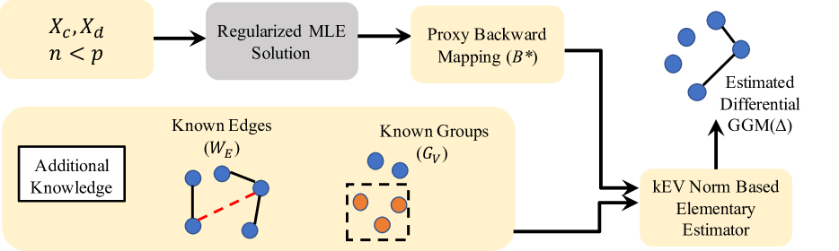
Figure 1: An overview of KDiffNet . KDiffNet integrates different types of extra knowledge for estimating differential GGMs using Elementary Estimators. As an example, the edge level knowledge can represent known edges (or non-edges) and group level knowledge represents information about multiple variables that function as groups.

Unfortunately, all previous differential network estimators rely on observed samples alone. Recent advances in data generation by genomics and neuroscience call for developing new dependency identification methods tailored to the integration of multiple sources of information and provide robust results in the high dimensional low sample regime. This paper fills the gap by proposing a novel method, namely KDiffNet , to add additional Knowledge in identifying DIFFerential Networks. By harnessing heterogeneous data across complementary sources, KDiffNet makes an essential step in enabling knowledge integration for differential dependency estimation beyond data samples. Figure 1 shows an overview of our method. This paper proposes KDiffNet plus multiple variations. We summarize our contributions as follows.

• Beyond data samples: KDiffNet is the first differential network estimator that can integrate multiple sources of evidence. We evaluate KDiffNet on more than 100 synthetic and multiple real-world datasets. KDiffNet consistently outperforms the state-of-the-art baselines and provides better down-stream prediction accuracy while achieving less or same time cost. Our experiments showcase how KDiffNet can integrate knowledge like known edges, anatomical grouping, and spatial evidence when estimating differential graph from heterogeneous multivariate samples (Section 3). We also design a meta-analysis strategy to avoid cases of mis-specified knowledge.

• Theoretically Sound: We theoretically prove the convergence error bounds of KDiffNet as $O(\sqrt{\frac{\log p}{\min(n_{c},n_{d})}})$ , achieving the same error bound as the state-of-the-art, improving under some conditions(Section 2.7). To the best of the authors’ knowledge, no known lower bounds about the convergence rate specifically under the additional knowledge setting were provided by the previous studies.

• Scalable: We design KDiffNet via an elementary estimator based framework and solve it using parallel proximal based optimization. KDiffNet scales to large $p$ and doesn’t need to design knowledge-specific optimization ( Section 2.5).

2 METHOD: KDiffNet

2.1 Basics and $\Delta$ As Canonical Parameter of Exponential Family

Estimating differential GGMs includes two sets of observed samples, denoted as two matrices $\mathbf{X}_{c}\in\mathbb{R}^{n_{c}\times p}$ and $\mathbf{X}_{d}\in\mathbb{R}^{n_{d}\times p}$. $\mathbf{X}_{c}$ and $\mathbf{X}_{d}$ assume i.i.d drawn from two normal distributions $N_{p}(\mu_{c},\Sigma_{c})$ and $N_{p}(\mu_{d},\Sigma_{d})$ respectively. Here $\mu_{c},\mu_{d}\in\mathbb{R}^{p}$ describe the mean vectors and $\Sigma_{c},\Sigma_{d}\in\mathbb{R}^{p\times p}$ represent covariance matrices. The goal of differential GGMs is to estimate the structural change $\Delta$ defined by Zhao et al. (2014) .

$$\vspace{-2.8mm}\Delta=\Omega_{d}-\Omega_{c}$$ (2.1)

Here $\Omega_{c}:=(\Sigma_{c})^{-1}$ and $\Omega_{d}:=(\Sigma_{d})^{-1}$ are two precision matrices. The sparsity pattern of the precision matrix of a GGM encodes the conditional dependency structure of the GGM. This means, $\Delta$ describes how the magnitude of conditional dependency differs between two conditions. A sparse $\Delta$ means few of its entries are non-zero, indicating a differential network with few edges.

A naive approach to estimate $\Delta$ will learn $\widehat{\Omega}_{d}$ and $\widehat{\Omega}_{c}$ from $\mathbf{X}_{d}$ and $\mathbf{X}_{c}$ independently and calculate $\widehat{\Delta}$ using Eq. (2.1). However, in a high-dimensional setting, the strategy needs to assume both $\Omega_{d}$ and $\Omega_{c}$ are sparse (to achieve consistent estimation of each) and has been found to produce many spurious differences de la Fuente (2010). The assumption of this two-step procedure is often not true. For instance, genetic networks contain hub nodes, therefore not entirely sparse Ideker and Krogan (2012). Recent literature in neuroscience has suggested that each subject’s functional brain connection network may not be sparse, though differences across subjects may be sparse Belilovsky et al. (2016).

Interestingly, the density ratio between two Gaussian distributions falls naturally in the exponential family (see detail proofs in  Section F.1). $\Delta$ is one entry of the canonical parameter of this exponential family distribution. According to Wainwright and Jordan (2008), learning an exponential family distribution from data means to estimate its canonical parameter. Computing the canonical parameter of an exponential family through vanilla MLE can be expressed as a backward mapping from given moments of the distribution Wainwright and Jordan (2008). In the case of differential GGM, the backward mapping (i.e., the vanilla MLE solution for $\Delta$) is a simple closed form: $\mathcal{B}(\widehat{\phi})=\mathcal{B}(\widehat{\Sigma}_{d},\widehat{\Sigma}_{c})=\big{(}\widehat{\Sigma}_{d}^{-1}-\widehat{\Sigma}_{c}^{-1})$, easily inferred from the two sample covariance matrices. $\widehat{\Sigma}$ denotes to the sample covariance matrix. However, when in high-dimensional regimes, $\mathcal{B}(\widehat{\Sigma}_{d},\widehat{\Sigma}_{c})$ is not well-defined because $\widehat{\Sigma}_{c}$ and $\widehat{\Sigma}_{d}$ are rank-deficient (thus not invertible). Here $\mathcal{B}$ refers to Backward Mapping. In next section, we design and use $\mathcal{B}^{*}$ that denotes proxy backward mapping (details later).

2.2 $\mathcal{R}(\cdot)$ Norm based Elementary Estimators (EE)

Multiple recent studies  Yang et al. (2014c, a, b); Wang et al. (2018b) followed a framework “Elementary estimators”:

$$\begin{split}&\mathop{\mathrm{argmin}}\limits_{\theta}\mathcal{R}(\theta),\\ &\text{Subject to: }\mathcal{R}^{*}(\theta-\widehat{\theta}_{n})\leq\lambda_{n}\end{split}$$ (2.2)

Where $\mathcal{R}(\cdot)$ represents a decomposable regularization function. $\mathcal{R}^{*}(\cdot)$ is the dual norm of $\mathcal{R}(\cdot)$,

$$\mathcal{R}^{*}(v):=\sup\limits_{u\neq 0}\frac{<u,v>}{\mathcal{R}(u)}=\sup\limits_{\mathcal{R}(u)\leq 1}<u,v>.$$ (2.3)

The design philosophy shared among elementary estimators is to construct $\widehat{\theta}_{n}$ carefully from well-defined estimators that are easy to compute and come with strong statistical convergence guarantees. For example, Yang et al. (2014a) conduct the high-dimensional estimation of $\ell_{1}$-regularized linear regression by using the classical ridge estimator as $\widehat{\theta}_{n}$ in Eq. (2.2). When $\widehat{\theta}_{n}$ itself is closed-form and $\mathcal{R}(\cdot)$ is the $\ell_{1}$-norm, the solution of Eq. (2.2) is naturally closed-form (as the dual norm of $\ell_{1}$ is $\ell_{\infty}$), therefore, easy and fast to compute, and scales to large $p$.

Following the above design philosophy, for our differential estimation task, $\Delta$ is the target canonical parameter $\theta$. We use a closed and well-defined form of $\widehat{\theta}_{n}$ (suggested by Wang et al. (2018b)):

$$\vspace{-4mm}\widehat{\theta}_{n}=\mathcal{B}^{*}(\widehat{\Sigma}_{d},\widehat{\Sigma}_{c})=\left([T_{v}(\widehat{\Sigma}_{d})]^{-1}-[T_{v}(\widehat{\Sigma}_{c})]^{-1}\right)$$ (2.4)

$\mathcal{B}^{*}(\widehat{\phi})$ denotes a so-called proxy of backward mapping for the target exponential family. Here $[T_{v}(A)]_{ij}:=\rho_{v}(A_{ij})$ where $\rho_{v}(\cdot)$ was chosen as a soft-thresholding function. Importantly, the formulation in Eq. (2.2) guarantees its solution to achieve a sharp convergence rate as long as $\widehat{\theta}_{n}$ is carefully chosen, well-defined, easy to compute and comes with a strong statistical convergence guarantee  Negahban et al. (2009). In summary, Eq. (2.2) provides an intriguing formulation to build simpler and possibly fast estimators accompanied by statistical guarantees. We, therefore, use it to design our method. To use Eq. (2.2) for estimating our target parameter $\Delta$, we need to design $\mathcal{R}(\Delta)$.

2.3 Integrating Complementary Sources of Knowledge via a new kEV Norm: $\mathcal{R}(\Delta)$

All previous estimators made the sparsity assumption and used $\ell_{1}$ norm to enforce the learned differential graph as sparse. However, there exist many other assumptions real-life tasks may prefer. Our main goal is to enable differential network estimators to integrate extra evidence beyond data samples. We group extra knowledge sources into two kinds: (1) edge-based, and (2) node-based.

(1) Knowledge as Weight Matrix: We propose to describe edge-level knowledge sources via positive weight matrices $W_{E}\in{\mathbb{R}}^{p\times p}$. We use $W_{E}$ via a weighted $\ell_{1}$ formulation $||W_{E}\circ\Delta||_{1}$. This enforces the prior that the larger a weight entry in $W_{E}$ is, the less likely the corresponding edge belongs to the true differential graph. None of the previous differential GGMs have explored this strategy.

The matrix $W_{E}$ can represent a good variety of prior knowledge. (1) For available hub nodes, we can design $W_{E}$ to assign all entries connecting to hubs with a smaller weight because genes tend to interact with hubs more, and hubs tend to get perturbed across conditions. (2) As another example, $W_{E}$ can describe spatial distance among brain regions (publicly available in sites like openfMRI (Poldrack et al., 2013)). This can nicely encode the domain prior that neighboring brain regions may be more likely to connect functionally. When considering two conditions like case vs. control, these spatially close nodes tend to be the vital differential edges. (3) Another important example is when identifying gene-gene interactions from expression profiles. Many state-of-the-art bio-databases like HPRD (Prasad et al., 2009) have collected information about direct “house-keeping” physical interactions between proteins. This type of interaction tends to happen across many conditions. So we can use $W_{E}$ to describe that known information, proposing corresponding sparse entries in the differential net.

In summary, the $W_{E}$ matrix-based representation provides a powerful and flexible strategy that allows integration of many possible forms of knowledge to improve differential network estimation, as long as they can be formulated via edge-level weights.

(2) Knowledge as Node Groups: Many real-world applications include knowledge about how variables group into sets. For example, biologists have collected a rich set of group evidence about how genes belong to various biological pathways or exist in the same or different cellular locations (Da Wei Huang and Lempicki, 2008). Gene grouping information provides solid biological bias that genes belonging to the same pathway tend to be co-activated or co-deactivated.

However, this type of group evidence cannot be described via the aforementioned $W_{E}$-based formulation. This is because it is safe to assume nodes in the same group share similar interaction patterns. However, we do not know beforehand if a specific group functions the same across two conditions (”group sparsity” – a block of sparse entries in the differential net) or differently between conditions (”dense sub-network” in the differential net).

To mitigate the issue, we propose to represent the group knowledge as a set of groups on feature variables (vertices) $\mathcal{G}_{p}$. Mathematically, $\forall g_{k}\in\mathcal{G}_{p}$, $g_{k}=\{i\}$ where $i$ indicates that the $i$-th node belongs to the group $k$. We propose integrating $\mathcal{G}_{p}$ knowledge into $\Delta$ by enforcing a group sparsity regularization on $\Delta$.

More specifically, we generate an “edge-group” index $\mathcal{G}_{V}$ from the node group index $\mathcal{G}_{p}$. This is done via defining $\mathcal{G}_{V}:=\{g^{\prime}_{k}|(i,j)\in g^{\prime}_{k},\forall i,\forall j\in g_{k}\}$. For vertex nodes in each node group $g_{k}$, all possible pairs between these nodes belong to an edge-group $g^{\prime}_{k}$. We propose to use the group,2 norm $||\Delta||_{\mathcal{G}_{V},2}$ to enforce group-wise sparse structure on $\Delta$. None of the previous differential GGM estimators have explored this knowledge-integration strategy.

kEV norm: Now we design $\mathcal{R}(\Delta)$ as a hybrid norm that combines the two strategies above. First, we assume that the true parameter $\Delta^{*}=\Delta^{*}_{e}+\Delta^{*}_{g}$: a superposition of two “clean” structures, $\Delta^{*}_{e}$ and $\Delta^{*}_{g}$. Then we define $\mathcal{R}(\Delta)$ as the “knowledge for Edges and Vertex norm (kEV-norm)”:

$$\mathcal{R}(\Delta)=||W_{E}\circ\Delta_{e}||_{1}+\epsilon||\Delta_{g}||_{\mathcal{G}_{V},2}$$ (2.5)

Here the Hadamard product $\circ$ denotes element-wise product between two matrices (i.e. $[A\circ B]_{ij}=A_{ij}B_{ij}$). $||\cdot||_{\mathcal{G}_{V},2}=\sum\limits_{k}||\Delta_{g^{\prime}_{k}}||_{2}$ and $k$ denotes the $k$-th group. The positive matrix $W_{E}\in R^{p\times p}$ describes one aforementioned edge-level additional knowledge. $\epsilon\geqslant 0$ is a hyperparameter. $\mathcal{R}(\Delta)$ is the superposition of edge-weighted $\ell_{1}$ norm and the group structured norm. Our target parameter $\Delta=\Delta_{e}+\Delta_{g}$.

2.4 kEV Norm based Elementary Estimator for identifying Differential Net:KDiffNet

kEV-norm has three desired properties (see proofs in Section E): (i) kEV-norm is a norm function if $\epsilon$ and entries of $W_{E}$ are positive. (ii) If the condition in (i) holds, kEV-norm is a decomposable norm. (iii) The dual norm of kEV-norm is $\mathcal{R}^{*}(u)$.

$$\mathcal{R}^{*}(u)=\max(||(1\varoslash W_{E})\circ u||_{\infty},\dfrac{1}{\epsilon}||u||^{*}_{\mathcal{G}_{V},2})$$ (2.6)

Here, $(1\varoslash W_{E})$ indicates the element wise division.

Now we define the proxy backward mapping using a closed-form formulation proposed by DIFFEE: $\widehat{\theta}_{n}=[T_{v}(\widehat{\Sigma}_{d})]^{-1}-[T_{v}(\widehat{\Sigma}_{c})]^{-1}$. Section F.4 proves that the chosen $\widehat{\theta}_{n}$ is theoretically well-behaved in high-dimensional settings.

Now by plugging $\mathcal{R}(\Delta)$, its dual $\mathcal{R}^{*}(\cdot)$ and $\widehat{\theta}_{n}$ into Eq. (2.2), we get the formulation of KDiffNet :

$$\begin{split}&\hskip 22.76219pt\mathop{\mathrm{argmin}}\limits_{\Delta}||W_{E}\circ\Delta_{e}||_{1}+\epsilon||\Delta_{g}||_{\mathcal{G}_{V},2}\\ &\text{Subject to: }\\ &||(1\varoslash W_{E})\circ\left(\Delta-\left([T_{v}(\widehat{\Sigma}_{d})]^{-1}-[T_{v}(\widehat{\Sigma}_{c})]^{-1}\right)\right)||_{\infty}\leq\lambda_{n}\\ &||\Delta-\left([T_{v}(\widehat{\Sigma}_{d})]^{-1}-[T_{v}(\widehat{\Sigma}_{c})]^{-1}\right)||^{*}_{\mathcal{G}_{V},2}\leq\epsilon\lambda_{n}\\ &\Delta=\Delta_{e}+\Delta_{g}\end{split}$$ (2.7)

2.5 Solving KDiffNet

We then design a proximal based optimization to solve Eq. (LABEL:eq:methodName_main), inspired by its distributed and parallel nature (Combettes and Pesquet, 2011). To simplify notations, we use $\Delta_{tot}:=[\Delta_{e};\Delta_{g}]$, where ; denotes the row wise concatenation. We also add three operator notations including $L_{e}(\Delta_{tot})=\Delta_{e}$, $L_{g}(\Delta_{tot})=\Delta_{g}$ and $L_{tot}(\Delta_{tot})=\Delta_{e}+\Delta_{g}$. Now we re-formulate KDiffNet as:

$$\begin{split}&\mathop{\mathrm{argmin}}\limits_{\Delta_{tot}}||W_{E}\circ(L_{e}(\Delta_{tot}))||_{1}+\epsilon||L_{g}(\Delta_{tot})||_{\mathcal{G}_{V},2}\\ &\text{subject to: }\\ &||(1\varoslash W_{E})\circ(L_{tot}(\Delta_{tot})-([T_{v}(\widehat{\Sigma}_{d})]^{-1}-[T_{v}(\widehat{\Sigma}_{c})]^{-1}))||_{\infty}\leq\lambda_{n}\\ &||L_{tot}(\Delta_{tot})-([T_{v}(\widehat{\Sigma}_{d})]^{-1}-[T_{v}(\widehat{\Sigma}_{c})]^{-1})||^{*}_{\mathcal{G}_{V},2}\leq\epsilon\lambda_{n}\\ \end{split}$$ (2.8)

Eq. (LABEL:eq:KDiffNet) used proxy backward mapping $\mathcal{B}^{*}(\widehat{\Sigma}_{d},\widehat{\Sigma}_{c}):=[T_{v}(\widehat{\Sigma}_{d})]^{-1}-[T_{v}(\widehat{\Sigma}_{c})]^{-1}$.

Algorithm 1 in Section C summarizes the Parallel Proximal algorithm (Combettes and Pesquet, 2011; Yang et al., 2014b) we propose for optimizing Eq. (LABEL:eq:distributed_main). Section C.2 further proves its computational cost as $O(p^{3})$. Detailed solutions for each proximal operator we proposed are summarized in Section C.

2.6 Variations and Meta Formulation

There exist many variations of KDiffNet .Closed-form Variations: (1) Edge Only or Group Only: For instance, we can estimate the target $\Delta$ through a closed form solution if we have only one kind of additional knowledge. Section C.3 provides the formulation and closed form solutions for edge-only or node-group-only cases. (2) DIFFEE as our special case: For the edge-only case, if we set $W_{E}$ as a matrix with all 1, Eq. (LABEL:eq:methodName_main) becomes the DIFFEE formulation. More Sets of Knowledge: (3) We also generalize KDiffNet to multiple kinds of group knowledge plus multiple sources of weight knowledge in Section D. Mis-specification: (4) When facing multiple types of evidence, misspecified evidence may exist for target goals. Section D.2 proposes strategies to use prediction performance to guide the selective use of extra evidence sources. Robust Covariance Estimation: (5) We also extend Eq. (LABEL:eq:methodName_main) with POET(Fan et al., 2013) based robust covariance estimations when the sample size is extremely small in real-world datasets like in our two virus related gene expression experiments.

2.7 Analysis of Error Bounds

In this section, Theorem $2.1$ provides a statistical analysis under the ‘KEV Norm’ structural constraints, leading to a non-probabilistic result that holds deterministically for all $\lambda_{n}$. Corollary $2.2$ provides the $asymptotic$ convergence rate in terms of how the error converges with number of dimensions $p$ and number of samples $n$, under KDiffNet’s distributional assumptions. KDiffNet achieves a sharp convergence rate, the same convergence rate $O(\sqrt{{(\log{p})}/{n}}))$ as DIFFEE. We borrow the following conditions defined in Yang et al. (2014c), regarding the decomposability of regularization function $\mathcal{R}$ with respect to the subspace pair $(\mathcal{M},\bar{\mathcal{M}}^{\perp})$:

(C1) $\mathcal{R}(u+v)=\mathcal{R}(u)+\mathcal{R}(v)$, $\forall u\in\mathcal{M},\forall v\in\bar{\mathcal{M}}^{\perp}$.

(C2) $\exists$ a subspace pair $(\mathcal{M},\bar{\mathcal{M}}^{\perp})$ such that the true parameter satisfies $\text{proj}_{\mathcal{M}^{\perp}}(\theta^{*})=0$

Now we introduce the following condition on ‘true’ ${\Delta}^{*}$: (EV-Sparsity): The ‘true’ ${\Delta}^{*}$ can be decomposed into two clear structures–$\{{\Delta_{e}}^{*}$ and ${\Delta_{g}}^{*}\}$. ${\Delta_{e}}^{*}$ is exactly sparse with $s_{E}$ non-zero entries indexed by a support set $S_{E}$ . ${\Delta_{g}}^{*}$ is exactly sparse with $\sqrt{s_{G}}$ non-zero groups (with at least one non-zero entry) indexed by a support set $S_{V}$. $S_{E}\bigcap S_{V}=\emptyset$. All other elements equal to $0$ (in $(S_{E}\bigcup S_{V})^{c}$).

Section I proves that kEV Norm satisfies conditions (C1) and (C2). This leads us to the following theorem (see proof  Section I):

Theorem 2.1.

Assuming $\Delta^{*}$ satisfies the condition (EV-Sparsity) and $\lambda_{n}\geq\mathcal{R}^{*}(\widehat{\Delta}-\Delta^{*})$, then the optimal point $\widehat{\Delta}$ has the following error bounds:

$$||\widehat{\Delta}-\Delta^{*}||_{F}\leq 4\max(\sqrt{s_{E}},\epsilon\sqrt{s_{G}})\lambda_{n}$$ (2.9)

We state the following conditions on the true canonical parameter under additional knowledge defining the class of differential GGMs: $\Delta^{*}=\Omega_{d}^{*}-\Omega_{c}^{*}$:

(C-MinInf$-\Sigma$): The true $\Omega_{c}^{*}$ and $\Omega_{d}^{*}$ of Eq. (2.1) have bounded induced operator norm i.e., $|||{\Omega_{c}}^{*}|||_{\infty}:=\sup\limits_{w\neq 0\in{\mathbb{R}}^{p}}\frac{||{\Omega_{c}}^{*}w||_{\infty}}{||w||_{\infty}}\leq W_{E_{min}}^{c*}\kappa_{1}$ and $|||{\Omega_{d}}^{*}|||_{\infty}:=\sup\limits_{w\neq 0\in{\mathbb{R}}^{p}}\frac{||{\Omega_{d}}^{*}w||_{\infty}}{||w||_{\infty}}\leq W_{E_{min}}^{d*}\kappa_{1}$. Here, intuitively, $W_{E_{min}}^{c*}$ corresponds to the largest ground truth weight index associated with non zero entries in $\Omega_{c}^{*}$. For set $S_{nz}=\{(i,j)|\Omega_{c_{ij}}^{*}=0\}$, $W_{E_{S_{nz}}}>W_{E_{min}}^{c*}$.

(C-Sparse-$\Sigma$): The two true covariance matrices $\Sigma_{c}^{*}$ and $\Sigma_{d}^{*}$ are “approximately sparse” (following Bickel and Levina (2008)). For some constant $0\leq q<1$ and $c_{0}(p)$, $\max\limits_{i}\sum\limits_{j=1}^{p}|[\Sigma_{c}^{*}]_{ij}|^{q}\leq c_{0}(p)$ and $\max\limits_{i}\sum\limits_{j=1}^{p}|[\Sigma_{d}^{*}]_{ij}|^{q}\leq c_{0}(p)$. We additionally require $\inf\limits_{w\neq 0\in{\mathbb{R}}^{p}}\frac{||\Sigma_{c}^{*}w||_{\infty}}{||w||_{\infty}}\geq\kappa_{2}$ and $\inf\limits_{w\neq 0\in{\mathbb{R}}^{p}}\frac{||\Sigma_{d}^{*}w||_{\infty}}{||w||_{\infty}}\geq\kappa_{2}$.

Using the above Theorem 2.1 and conditions, we have the following corollary about the convergence rate of KDiffNet (see its proof in Section G.2.2).

Corollary 2.2.

In the high-dimensional setting, i.e., $p>\max(n_{c},n_{d})$, let $v:=a\sqrt{\frac{\log p}{\min(n_{c},n_{d})}}$. Then for $\lambda_{n}:=\frac{\Gamma\kappa_{1}a}{4\kappa_{2}}\sqrt{\frac{\log p}{\min(n_{c},n_{d})}}$ and $\min(n_{c},n_{d})>c\log p$, with a probability of at least $1-2C_{1}\exp(-C_{2}p\log(p))$, the estimated optimal solution $\widehat{\Delta}$ has the following error bound:

$$\vspace{-4mm}||\widehat{\Delta}-\Delta^{*}||_{F}\leq\frac{\Gamma a\max((\sqrt{s}_{E}),\epsilon\sqrt{s_{G}})}{\kappa_{2}}\sqrt{\frac{\log p}{\min(n_{c},n_{d})}}$$ (2.10)

Here $\Gamma=32\kappa_{1}\dfrac{\max(W_{E_{\min}}^{c*},W_{E_{\min}}^{d*})}{W_{E_{\min}}}$, where $a$, $c$,$C_{1}$, $C_{2}$, $\kappa_{1}$ and $\kappa_{2}$ are constants. $a$ depends on $\max_{i}\Sigma_{ii}^{*}$ and $c$ depends on $p,\tau,\max_{i}\Sigma_{ii}^{*}$. $\tau$ is a constant from Lemma 1 of Ravikumar et al. (2011).

We can prove that under the same conditions above, DIFFEE achieves the same asymptotic convergence rate as Eq. (2.10). However its rate includes a different constant $\Gamma=32\kappa_{1}{\max(W_{E_{\min}}^{c*},W_{E_{\min}}^{d*})}$. Notably, when $W_{E_{\min}}>1$, KDiffNet converging constant is better than DIFFEE. We have also included theoretical results when under misspecification assumptions and when using POET robust covariance estimation in Section I.

2.8 Connecting to Relevant GGM Studies beyond Data Samples

To the authors’ best knowledge, only two loosely-related studies exist in the literature to incorporate edge-level knowledge for other types of GGM estimation. (1) One study with the name NAK  (Bu and Lederer, 2017) (following ideas from Shimamura et al. (2007)) proposed to integrate Additional Knowledge into the estimation of single-task graphical model via a weighted Neighbourhood selection formulation. (2) Another study with the name JEEK (Wang et al., 2018a) (following Singh et al. (2017)) considered edge-level evidence via a weighted objective formulation to estimate multiple dependency graphs from heterogeneous samples. Both studies only added edge-level extra knowledge in structural learning and neither of the approaches was designed for direct differential structure estimation. Besides, JEEK uses a multi-task formulation.

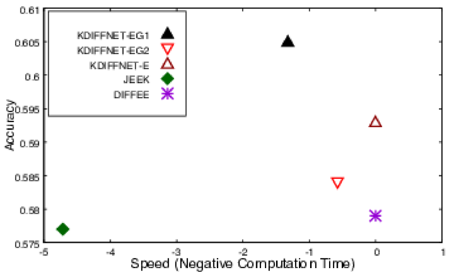
(a) Classification Performance comparison on ABIDE Dataset: KDiffNet-EG achieves highest Accuracy (averaged over $3$ random seeds) without sacrificing computation speed (points towards top right are better).

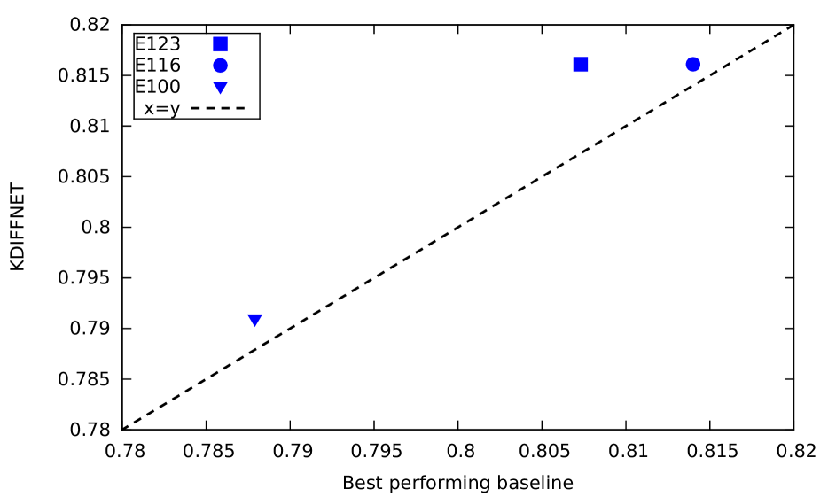
(b) Classification Performance on three Epigenomic Datasets: KDiffNet-E achieves highest Accuracy (averaged over $3$ splits) in comparison to the best performing baseline. (points above the diagonal dashed line indicate ours is better).

(c) Edge-recovery Performance: F1-Score vs number of perturbed hub nodes. Real-life genetic networks include hub nodes that are being targeted the most by external stimulus (i.e. perturbed hubs).

Figure 2: Classification Results for (a) Real-world Brain data (ABIDE) and (b) Real-world epigenetic datasets, (c) Edge Recovery Accuracy for Simulation Data for Perturbed Nodes.

3 EXPERIMENTS

Datasets: We compare KDiffNet , variations and baselines on multiple datasets: (1) A total of $126$ different synthetic datasets representing various combinations of additional knowledge and hyper-parameter sensitivity analysis; and, (2) One fMRI dataset (ABIDE) for functional brain connectivity estimation,(3) Three epigenomic datasets for differential epigenetic network estimation, (4) Two gene expression datasets on virus (including SARS-CoV-2) infected and mock control samples for differential genetic network estimation. Results on virus related gene network identification and validation are in Section L.2.

Baselines: We compare KDiffNet to estimators with additional knowledge: (1) JEEK(Wang et al., 2018a), (2) NAK(Bu and Lederer, 2017), and estimators without any external evidence: (3) SDRE (Liu et al., 2017), (4) DIFFEE (Wang et al., 2018b) and (5) JGLFUSED(Danaher et al., 2013). We also check two variations of KDiffNet : KDiffNet-E using only edge knowledge and KDiffNet-G using only group knowledge ( Section C.3).

Metrics: For simulation datasets, we evaluate the methods in terms of edge-level F1-Score. For the real-world datasets, due to lack of access to the ground truth $\Delta^{*}$, we use test accuracy obtained using pairwise quadratic features(obtained from the edges in the difference matrix) as linear predictors.

Hyperparameters: We tune the key hyper-parameters:

• $v$ : To compute the proxy backward mapping, we vary $v$ in $\{0.001i|i=1,2,\dots,1000\}$ (to make $T_{v}(\Sigma_{c})$ and $T_{v}(\Sigma_{d})$ invertible).

• $\lambda_{n}$ : According to our convergence rate analysis in Section 2.7, $\lambda_{n}\geq C\sqrt{\frac{\log p}{\min(n_{c},n_{d})}}$, we choose $\lambda_{n}$ from a range of $\{0.01\times\sqrt{\frac{\log p}{\min(n_{c},n_{d})}}\times i|i\in\{1,2,3,\dots,100\}\}$ using cross-validation. For KDiffNet-G , we tune over $\lambda_{n}$ from a range of $\{0.1\times\sqrt{\frac{\log p}{\min(n_{c},n_{d})}}\times i|i\in\{1,2,3,\dots,100\}\}$.

• $\epsilon$: For KDiffNet-EG , we tune $\epsilon\in\{0.0001,0.01,1,100\}$.

3.1 Experiment 1: Simulation Datasets

In the following subsections, we present details about the data generation, followed by results under multiple settings.

Data Generation

:For overlapping Edge and Vertex Knowledge (KEG), we generate simulated datasets (Data-EG) with a clear underlying differential structure between two conditions. We simulate the case of overlapping group and edge knowledge. We select the block diagonals of size $m$ as groups in $\Delta^{g}$. If two variables $i,j$ are in a group $g^{\prime}$, in $\Delta^{g}_{ij}=1/3$, else $\Delta^{g}_{ij}=0$, where $\Delta^{g}\in{\mathbb{R}}^{p\times p}$. For the edge-level knowledge component, given a known weight matrix $W_{E}$, we set $W^{d}=inv.logit(-W_{E})$. Higher the value of $W_{E_{ij}}$, lower the value of $W^{d}_{ij}$, hence lower the probability of that edge to occur in the true precision matrix. We select different levels in the matrix $W^{d}$, denoted by $s$, where if $W^{d}_{ij}>s_{l}$, we set $\Delta^{d}_{ij}=1/3$, else $\Delta^{d}_{ij}=0$. ${B}_{I}$ is a random graph with each edge ${B}_{{I}_{ij}}=1/3$ with probability $p$. ${\Omega}_{d}=\Delta^{d}+\Delta^{g}+{B}_{I}+\delta_{d}I$, ${\Omega}_{c}={B}_{I}+\delta_{c}I$, finally, ${\Delta}={\Omega}_{d}-{\Omega}_{c}$. $\delta_{c}$ and $\delta_{d}$ are selected large enough to guarantee positive definiteness. We generate two blocks of data samples following Gaussian distribution using $N(0,{\Omega}_{c}^{-1})$ and $N(0,{\Omega}_{d}^{-1})$. We use these data samples only to approximate the differential GGM to compare to the ground truth ${\Delta}$. For the other data settings(Data-G and Data-E), we have provided details in Section M.

3.1.1 Results on Simulation Experiments

Method	Data-EG(Time)	Data-EG(F1-Score)			Data-G(Time)	Data-G(F1-Score)
	W2($p=246$)	W1($p=116$)	W2($p=246$)	W3($p=160$)	W2($p=246$)	W2($p=246$)
KDiffNet-EG	3.270$\pm$0.182	0.704$\pm$0.022	0.926$\pm$0.001	0.934$\pm$0.002	*	*
KDiffNet-G	0.006$\pm$0.00	0.578$\pm$0.001	0.565$\pm$0.00	0.576$\pm$0.00	0.006$\pm$0.000	0.860$\pm$0.000
KDiffNet-E	0.005$\pm$0.001	0.686$\pm$0.024	0.918$\pm$0.001	0.916$\pm$0.002	*	*
JEEK (Wang et al., 2018a)	10.476$\pm$0.054	0.571$\pm$0.010	0.582$\pm$0.001	0.582$\pm$0.001	*	*
NAK(Bu and Lederer, 2017)	6.520$\pm$0.184	0.225$\pm$0.013	0.198$\pm$0.011	0.203$\pm$0.005	*	*
SDRE(Liu et al., 2014)	28.807$\pm$1.673	0.573$\pm$0.11	0.568$\pm$0.006	0.574$\pm$0.11	11.764$\pm$1.23	0.318$\pm$0.10
DIFFEE(Wang et al., 2018b)	0.005$\pm$0.00	0.570$\pm$0.001	0.562$\pm$0.00	0.570$\pm$0.00	0.004$\pm$0.000	0.131$\pm$0.131
JGLFUSED(Danaher et al., 2013)	109.15$\pm$13.659	0.512$\pm$0.001	0.489$\pm$0.001	0.504$\pm$0.001	112.441$\pm$6.362	0.060$\pm$0.00
Number of Datasets	14	14	14	14	14	14

Table 1: Mean Performance(F1-Score) and Computation Time(seconds) with standard deviation for $10$ random seeds given in parentheses of KDiffNet-EG , KDiffNet-E , KDiffNet-G and baselines for simulated data. We evaluate over $126$ datasets: $14$ variations in each of the three spatial matrices $W_{E}$: $p=116$(W1), $p=246$(W2), and $p=160$(W3) for the three data settings: Data-EG, Data-E and Data-G. $*$ indicates that the method is not applicable for a data setting.

We present a summary of our results (partial) in Table 1: the columns representing two cases of data generation settings (Data-EG and Data-G). Table 1 uses the $mean$ F1-score (across different settings of $p$, $n_{c}$, $n_{d}$, etc.) and the computational time cost to compare methods (rows). We repeat each experiment for $10$ random seeds. We can make several conclusions:

(1) KDiffNet outperforms baselines that do not consider knowledge. Clearly, KDiffNet and its variations achieve the highest F1-score across all the $126$ datasets. SDRE and DIFFEE are differential network estimators but perform poorly indicating that adding additional knowledge improves differential GGM estimation. MLE-based JGLFUSED performs the worst in all cases.

(2) KDiffNet outperforms the baselines that consider knowledge, especially when group knowledge exists. When under the Data-EG setting, while JEEK and NAK include the extra edge information, they cannot integrate group information and are not designed for differential estimation. This results in lower F1-Score (0.582 and 0.198 for W2) compared to KDiffNet-EG (0.926 for W2). The advantage of utilizing both edge and node groups evidence is also indicated by the higher F1-Score of KDiffNet-EG with respect to KDiffNet-E and KDiffNet-G on the Data-EG setting (Top 3 rows in Table 1). On Data-G cases, none of the baselines can model node group evidence. On average KDiffNet-G performs $6.4\times$ better than the baselines for $p=246$ with respect to F1.

(3) KDiffNet achieves reasonable time cost versus the baselines and is scalable to large $p$. Figure 11 shows each method’s time cost per $\lambda_{n}$ for large $p=2000$. KDiffNet-EG is faster than JEEK, JGLFUSED and SDRE (Column 1 in Table 1). KDiffNet-E and KDiffNet-G are faster than KDiffNet-EG owing to closed form solutions. On Data-G dataset and Data-E datasets, our faster closed form solutions are able to achieve more computational speedup. For example, on datasets using W2 $p=246$, KDiffNet-E and KDiffNet-G are on an average $21000\times$ and $7400\times$ faster (Column 5 in Table 1) than the baselines, respectively.

(4) KDiffNet-G outperforms baselines on Knowledge of the perturbed hub nodes In Figure 2(c), we consider the scenario when a group of nodes is perturbed in the case condition relative to the control condition. Details for the data generation are in  N.7. KDiffNet-G can directly take into account the group of perturbed nodes and hence shows the best performance when compared to the baselines.

(5) KDiffNet-EG outperforms the baselines irrespective of hyperparameter $\lambda_{n}$ choice: Besides F1-Score, we also analyze KDiffNet ’s performance when varying hyper-parameter $\lambda_{n}$ using ROC curves. KDiffNet achieves the highest Area under Curve (AUC) in comparison to all other baselines, indicating it is not sensitive to varying hyperparameters. In  Section M , we use three different subsections to present more analysis results for all the $126$ datasets under the three different data simulation settings.

(6) KDiffNet-EG outperforms deep learning based structure learning methods: In N.1, we compare edge recovery of KDiffNet against state-of-the-art deep learning models that can learn graph structure from data. Table 5 and Table 6 indicate that in such high dimensional cases, deep models are not able to learn the correct differential structures, as indicated by lower F1 score.

3.2 Experiment 2: Human Brain Connectivity from fMRI

Real world scientific datasets present unique challenges and opportunities for structure discovery. While their ground truth graphs are unknown, experimental studies have led to a plethora of disparate external sources of structure evidence. We evaluate KDiffNet in a real-world downstream classification task on a publicly available resting-state fMRI dataset: ABIDE(Di Martino et al., 2014). The ABIDE data aims to understand human brain connectivity and how it reflects neural disorders (Van Essen et al., 2013).

Data Processing: The data is retrieved from the Preprocessed Connectomes Project (Craddock, 2014). ABIDE includes two groups of human subjects: autism and control. After preprocessing with Configurable Pipeline for the Analysis of Connectomes (CPAC) (Craddock et al., 2013) pipeline, $871$ individuals remain ($468$ diagnosed with autism). Signals for the 160 (number of features $p=160$) regions of interest (ROIs) in the often-used Dosenbach Atlas (Dosenbach et al., 2010) are examined.

Sources of Additional Knowledge: We utilize three types of collated evidence in neuroscience: first, as spatially distant regions are less likely to be connected in the brain(Watts and Strogatz, 1998; Vértes et al., 2012), we employ $W_{E}$ derived from the spatial distance between $160$ brain regions of interest(ROI) (Dosenbach et al., 2010). Further, scientists have classified two types of groups of brain regions that behave similarly(functionally or connective) from Dosenbach Atlas(Dosenbach et al., 2010): (1) macroscopic brain structures with $40$ unique groups (G1) and (2) $6$ higher level node groups having the same functional connectivity(G2).

Results: To evaluate the learnt differential structure in the absence of a ground truth graph, we utilize the non-zero edges from the estimated graph in downstream classification. The subjects are randomly partitioned into three equal sets: a training set, a validation set, and a test set. Each estimator produces $\widehat{\Omega}_{c}-\widehat{\Omega}_{d}$ using the training set. Then, the nonzero edges in the difference graph are used for feature selection. Namely, for every edge between ROI x and ROI y, the mean value of $x\times y$ over time was selected as a feature. These features are fed to a logistic regressor with ridge penalty, which is tuned via cross-validation. Accuracy is reported on the test set. For all methods, we tune $\lambda_{n}$ to vary the fraction of zero edges(non-edges) of the inferred graphs from $0.01\times i|i\in\{50,51,52,\dots,70\}$. We repeat the experiment for $3$ random seeds and report the average test accuracy. Figure 2(a) compares KDiffNet-EG and baselines on ABIDE, using the $y$ axis for classification test accuracy (the higher the better) and the $x$ axis for the computation speed per $\lambda_{n}$ (negative seconds, the more right the better). KDiffNet -EG1, incorporating both edge($W_{E}$) and (G1) group knowledge, achieves the highest accuracy of $60.5\%$ for distinguishing the autism vs the control subjects without sacrificing computation speed. We show the learnt differential network in Figure 3.

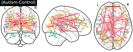
Figure 3: Differential Graph (of three views) between Autism and Control visualized using nilearn package.

3.3 Experiment 3: Epigenetic Network from Histone Modifications

In this experiment, we evaluate KDiffNet and baselines for estimating the differential epigenetic network between low and high gene expression. Cellular diversity is attributed to cell type-specific patterns of gene expression, in turn associated with a complex regulation mechanism. Studies have shown that epigenetic factors(like histone modifications(HMs)), act combinatorially to regulate gene expression (Suganuma and Workman, 2008; Berger, 2007).

Data Processing: We consider five core HM marks (H3K4me3, H3K4me1, H3K36me3, H3K9me3, H3K27me3) and three major cell types(K562 Leukemia Cells(E123), GM12878 Lymphoblastoid Cells(E116) and Psoas Muscle(E100)) with genome-level gene expression profiled in the REMC database (Kundaje et al., 2015).

Sources of Additional Knowledge: Signals closer to each other relative to the transcription start site for each gene are more likely to interact in the gene regulation process. We design a $W_{E}$ matrix based on this genomic distance.

Results: Figure 2(b) reports the average test set performance(average across $3$ data splits) for the three cell types. We plot the test accuracy achieved by KDiffNet on the $y-$axis, with the best performing baseline on the $x-$axis. KDiffNet outperforms DIFFEE that does not use $W_{E}$ as well as JEEK, that can incorporate this information but estimates the two networks separately. Figure 5 shows a qualitative comparison of the epigenetic networks learnt by KDiffNet and DIFFEE.

4 CONCLUSIONS

In this paper, we show that KDiffNet is flexible in incorporating different kinds of available evidence, leading to improved differential network estimation, without additional computational cost and can improve downstream tasks like classification. We believe the flexibility and scalability provided by KDiffNet can be beneficial in many real-world tasks. We plan to generalize from Gaussian to semi-parametric distributions or to Ising models next.

 

Supplementary Material:
Beyond Data Samples: Aligning Differential Networks Estimation with Scientific Knowledge

 

Part A: Supplementary Materials for Optimization, Error Bounds, Proofs and Theoretical Backgrounds

Appendix A CONNECTING TO DIFFERENTIAL GGM FORMULATIONS

Recent literature includes multiple differential network estimators to go beyond the naive strategy. They roughly fall into four categories (Section 1). We present one estimator from each group here.

Multitask MLE based: JGLFused: One study ”Joint Graphical Lasso” (JGL) (Danaher et al., 2013) used multi-task MLE formulation for joint learning of multiple sparse GGMs. JGL can estimate a differential network when using an additional sparsity penalty called the fused norm:

$$\begin{split}\mathop{\mathrm{argmin}}\limits_{\Omega_{c},\Omega_{d}\succ 0,\Delta}&n_{c}(-\log\text{det}(\Omega_{c})+<\Omega_{c},\widehat{\Sigma}_{c}>)\\ +&n_{d}(-\log\text{det}(\Omega_{d})+<\Omega_{d},\widehat{\Sigma}_{d}>)\\ +&\lambda_{2}(||\Omega_{c}||_{1}+||\Omega_{d}||_{1})+\lambda_{n}||\Delta||_{1}\end{split}$$ (A.1)

Another study (Honorio and Samaras, 2010) used $\ell_{1}$/$\ell_{\infty}$ regularization via a similar multi-task MLE formulation. Studies in this group jointly learn two GGMs and the difference. However, these multi-task methods do not work if each graph is dense but the change is sparse.

Density ratio based: SDRE: Liu et al. (2014) proposed to directly estimate Sparse differential networks for exponential family by Density Ratio Estimation:

$$\mathop{\mathrm{argmax}}\limits_{\Delta}\mathcal{L}_{\text{KLIEP}}(\Delta)-\lambda_{n}\parallel\Delta\parallel_{1}-\lambda_{2}\parallel\Delta\parallel_{2}$$ (A.2)

$\mathcal{L}_{\text{KLIEP}}$ minimizes the KL divergence between the true probability density $p_{d}(x)$ and the estimated without explicitly modeling the true $p_{c}(x)$ and $p_{d}(x)$. This estimator uses the elastic-net penalty for enforcing sparsity.

Constrained $\ell_{1}$ minimization based: Diff-CLIME: The study by Zhao et al. (2014) directly learns $\Delta$ through a constrained optimization formulation.

$$\begin{split}&\mathop{\mathrm{argmin}}\limits_{\Delta}||\Delta||_{1}\\ \text{Subject to: }&||\widehat{\Sigma}_{c}\Delta\widehat{\Sigma}_{d}-(\widehat{\Sigma}_{c}-\widehat{\Sigma}_{d})||_{\infty}\leq\lambda_{n}\end{split}$$ (A.3)

The optimization reduces to multiple linear programming problems with a computational complexity of $O(p^{8})$. This method doesn’t scale to large $p$.

Elementary estimator based: DIFFEE: EE based UGM estimator from Yang et al. (2014c) proposed the following generic formulation to estimate canonical parameter for an exponential family distribution via EE framework:

$$\begin{split}\mathop{\mathrm{argmin}}\limits_{\theta}||\theta||_{1},\hskip 8.53581pt\text{Subject to: }||\theta-\mathcal{B}^{*}(\widehat{\phi})||_{\infty}\leq\lambda_{n}\end{split}$$ (A.4)

For an exponential family distribution, $\theta$ is its canonical parameter to learn. Wang et al. (2018b) proposed a so-called DIFFEE for estimating sparse structure changes in high-dimensional GGMs directly:

$$\begin{split}&\mathop{\mathrm{argmin}}\limits_{\Delta}||\Delta||_{1,,\text{off}}\\ \text{Subject to: }&||\Delta-\mathcal{B}^{*}(\widehat{\Sigma}_{d},\widehat{\Sigma}_{c})||_{\infty,\text{off}}\leq\lambda_{n}\end{split}$$ (A.5)

The design of Wang et al. (2018b) follows a so-called family of elementary estimators. We explain details of $\mathcal{B}^{*}(\widehat{\Sigma}_{d},\widehat{\Sigma}_{c})$ in Section 2.2. DIFFEE’s solution is a closed-form entry-wise thresholding operation on $\mathcal{B}^{*}(\widehat{\Sigma}_{d},\widehat{\Sigma}_{c})$ to ensure the desired sparsity structure of its final estimate. Here $\lambda_{n}>0$ is the tuning parameter. Empirically, DIFFEE scales to large $p$ and is faster than SDRE and Diff-CLIME.

Eq. (A.5) is a special case of Eq. (2.2), in which $\mathcal{R}(\cdot)$ is the $\ell_{1}$-norm for enforcing sparsity. The differential network $\Delta$ is the $\theta$ in Eq. (2.2) that we aim to estimate. $\mathcal{R}^{*}(\cdot)$ in Eq. (A.5) is the dual norm of $\ell_{1}$, therefore Eq. (A.5) used $\ell_{\infty}$.

DIFFEE: Eq. (A.5) is a special case of Eq. (A.4). Eq. (A.4) is a special case of Eq. (2.2).

Appendix B MORE DETAILS OF RELEVANT STUDIES BEYOND DATA SAMPLES

NAK (Bu and Lederer, 2017): For the single task sGGM, one recent study (Bu and Lederer, 2017) (following ideas from Shimamura et al. (2007)) proposed to use a weighted Neighborhood selection formulation to integrate edge-level Additional Knowledge (NAK) as: $\widehat{\beta}^{j}=\mathop{\mathrm{argmin}}\limits_{\beta,\beta_{j}=0}\frac{1}{2}||\bm{X}^{j}-\bm{X}\beta||_{2}^{2}+||\mathbf{r}_{j}\circ\beta||_{1}$. Here $\widehat{\beta}^{j}$ is the $j$-th column of a single sGGM $\widehat{\Omega}$. Specifically, $\widehat{\beta}^{j}_{k}=0$ if and only if $\widehat{\Omega}_{k,j}=0$. $\mathbf{r}_{j}$ represents a weight vector designed using available extra knowledge for estimating a brain connectivity network from samples $\bm{X}$ drawn from a single condition. The NAK formulation can be solved by a classic Lasso solver like glmnet.

JEEK(Wang et al., 2018a): Two related studies, JEEK(Wang et al., 2018a) and W-SIMULE(Singh et al., 2017) incorporate edge-level extra knowledge in the joint discovery of $K$ heterogeneous graphs. In both these studies, each sGGM corresponding to a condition $i$ is assumed to be composed of a task specific sGGM component $\Omega^{(i)}_{I}$ and a shared component $\Omega_{S}$ across all conditions, i.e., $\Omega^{(i)}=\Omega^{(i)}_{I}+\Omega_{S}$. The minimization objective of W-SIMULE is as follows: objective:

$$\mathop{\mathrm{argmin}}\limits_{\Omega^{(i)}_{I},\Omega_{S}} \sum\limits_{i}||W\circ\Omega^{(i)}_{I}||_{1}+\epsilon K||W\circ\Omega_{S}||_{1}$$ (B.1)

subject to: $$||\Sigma^{(i)}(\Omega^{(i)}_{I}+\Omega_{S})-I||_{\infty}\leq\lambda_{n},\;i=1,\dots,K$$

W-SIMULE is very slow when $p>200$ due to the expensive computation cost $O(K^{4}p^{5})$. In comparison, JEEK is an EE-based optimization formulation:

$$\begin{split}\mathop{\mathrm{argmin}}\limits_{\Omega^{tot}_{I},\Omega^{tot}_{S}}&||W^{tot}_{I}\circ\Omega^{tot}_{I}||_{1}+||W^{tot}_{S}\circ\Omega^{tot}_{S}||\\ \text{ subject to: }&||\dfrac{1}{W^{tot}_{I}}\circ(\Omega^{tot}-B^{*}(\widehat{\phi})))||_{\infty}\leq\lambda_{n}\\ &||\dfrac{1}{W^{tot}_{S}}\circ(\Omega^{tot}-B^{*}(\widehat{\phi}))||_{\infty}\leq\lambda_{n}\\ &\Omega^{tot}=\Omega^{tot}_{S}+\Omega^{tot}_{I}\end{split}$$ (B.2)

Here, $\Omega_{I}^{tot}=(\Omega_{I}^{(1)},\Omega_{I}^{(2)},\dots,\Omega_{I}^{(K)})$ and $\Omega_{S}^{tot}=(\Omega_{S},\Omega_{S},\dots,\Omega_{S})$. The edge knowledge of the task-specific graph is represented as weight matrix $\{W^{(i)}\}$ and $W_{S}$ for the shared network. JEEK differs from W-SIMULE in its constraint formulation, that in turn makes its optimization much faster and scalable than WSIMULE. In our experiments, we use JEEK as our baseline.

Drawbacks: However, none of these studies are flexible to incorporate other types of additional knowledge like node groups or cases where overlapping group and edge knowledge are available for the same target parameter. Further, these studies are limited by the assumption of sparse single condition graphs. Estimating a sparse difference graph directly is more flexible as it does not rely on this assumption.

B.1 Related Work on Genetic Network Identification

A genetic interaction network describes biological interactions among genes and provides a systematic understanding of how components communicate and influence each other during cellular signaling and regulatory processes. To reverse engineer genetic networks from observed gene expression profiles (like from multiple tissue samples), the bioinformatics literature includes methods from four categories:

• (a) Correlation and partial correlation based methods(Schäfer and Strimmer, ; Meinshausen and Bühlmann, 2006). Correlation networks are vulnerable to false positives. Partial correlation based probabilistic GGMs (Dobra et al., 2004; Allen and Liu, 2013) successfully avoid this problem with some additional assumptions like Gaussianity. This has been shown to be a reasonable assumption in case of inferring genetic networks from gene expression data.

• (b) Regression based approaches (Vân Anh Huynh-Thu et al., 2010; Haury et al., 2012). These suffer from poor performance in the cases of limited data.

• (c) Bayesian Networks(Mukherjee and Speed, 2008; Werhli and Husmeier, ): These are probabilistic graphical models representing conditional dependencies in the form of Directed Acyclic Graphs. Bayesian network based methods are limited in how scalable they are, especially when facing high-dimensional genome-wide data sets;

• (d) Information theory based or non-parametric based models. They measure non linear associations(Zhang et al., 2012, 2015; Margolin et al., 2006; Meyer et al., 2007).

• Some recent methods also focus on Differential Genetic Network Analysis. (Yu et al., 2011) proposed to identify differential gene pairs of co-expression networks. (Zhang et al., 2016) inferred differential correlation-based networks by decomposing them to global and group-specific components.

Appendix C OPTIMIZATION OF KDiffNet AND ITS VARIANTS

In summary, the three added operators are affine mappings and can write as: $L_{e}=A_{e}\Delta_{tot}$, $L_{g}=A_{g}\Delta_{tot}$, and $L_{tot}=A_{tot}\Delta_{tot}$, where $A_{e}=[\bm{I}_{p\times p}\quad\bm{0}_{p\times p}]$, $A_{g}=[\bm{0}_{p\times p}\quad\bm{I}_{p\times p}]$ and $A_{tot}=[\bm{I}_{p\times p}\quad\bm{I}_{p\times p}]$.

Now we reformulate Eq. (LABEL:eq:KDiffNet) to the following equivalent and distributed formulation:

$$\begin{split}&\mathop{\mathrm{argmin}}\limits_{\Delta_{tot}}F_{1}(\Delta_{{tot}_{1}})+F_{2}(\Delta_{{tot}_{2}})+G_{1}(\Delta_{{tot}_{3}})+G_{2}(\Delta_{{tot}_{4}})\\ &\text{subject to: }\Delta_{{tot}_{1}}=\Delta_{{tot}_{2}}=\Delta_{{tot}_{3}}=\Delta_{{tot}_{4}}=\Delta_{tot}\end{split}$$ (C.1)

Where $F_{1}(\cdot)=||W_{E}\circ(L_{e}(\cdot))||_{1}$, $G_{1}(\cdot)=\mathcal{I}_{||(1\varoslash W_{E})\circ\left(L_{tot}(\cdot)-\mathcal{B}^{*}(\widehat{\Sigma}_{d},\widehat{\Sigma}_{c})\right)||_{\infty}\leq\lambda_{n}}$, $F_{2}(\cdot)=\epsilon||L_{g}(\cdot)||_{\mathcal{G}_{V},2}$ and $G_{2}(\cdot)=\mathcal{I}_{||L_{tot}(\cdot)-\mathcal{B}^{*}(\widehat{\Sigma}_{d},\widehat{\Sigma}_{c})||^{*}_{\mathcal{G}_{V},2}\leq\epsilon\lambda_{n}}$. Here $\mathcal{I}_{C}(\cdot)$ represents the indicator function of a convex set $C$ denoting that $\mathcal{I}_{C}(x)=0$ when $x\in C$ and otherwise $\mathcal{I}_{C}(x)=\infty$.

Algorithm 1 Parallel Proximal Algorithm for KDiffNet

0:  Two data matrices $\mathbf{X}_{c}$ and $\mathbf{X}_{d}$, The weight matrix $W_{E}$ and $\mathcal{G_{V}}$. Hyperparameters: $\alpha$, $\epsilon$, $v$, $\lambda_{n}$ and $\gamma$. Learning rate: $0<\rho<2$. Max iteration number $iter$.

0:  $\Delta$

1:  Compute $\mathcal{B}^{*}(\widehat{\Sigma}_{d},\widehat{\Sigma}_{c})$ from $\mathbf{X}_{d}$ and $\mathbf{X}_{c}$

2:  Initialize $A_{e}=[\bm{I}_{p\times p}\quad\bm{0}_{p\times p}]$, $A_{g}=[\bm{0}_{p\times p}\quad\bm{I}_{p\times p}]$, $A_{tot}=[\bm{I}_{p\times p}\quad\bm{I}_{p\times p}]$,

3:  Initialize $\Delta_{{tot}_{1}}$, $\Delta_{{tot}_{2}}$, $\Delta_{{tot}_{3}}$, $\Delta_{{tot}_{4}}$ and $\Delta_{{tot}}=\dfrac{\Delta_{{tot}_{1}}+\Delta_{{tot}_{2}}+\Delta_{{tot}_{3}}+\Delta_{{tot}_{4}}}{4}$

4:  for $i=0$ to $iter$ do

5:     $p^{i}_{1}=\text{prox}_{4\gamma F_{1}}\Delta_{{tot}_{1}}^{i}$; $p^{i}_{2}=\text{prox}_{4\gamma F_{2}}\Delta_{{tot}_{2}}^{i}$; $p^{i}_{3}=\text{prox}_{4\gamma G_{1}}\Delta_{{tot}_{3}}^{i}$; $p^{i}_{4}=\text{prox}_{4\gamma G_{2}}\Delta_{{tot}_{4}}^{i}$

6:     $p^{i}=\frac{1}{4}(\sum\limits_{j=1}^{4}p_{j}^{i})$

7:     for $j=1,2,3,4$ do

8:        $\Delta_{{tot}_{j}}^{i+1}=\Delta_{{tot}}^{i}+\rho(2p^{i}-\Delta^{i}_{{tot}}-p_{j}^{i})$

9:     end for

10:     $\Delta_{tot}^{i+1}=\Delta^{i}_{tot}+\rho(p^{i}-\Delta_{tot}^{i})$

11:  end for

12:  $\widehat{\Delta}=A_{tot}\Delta_{tot}^{iter}$

12:  $\widehat{\Delta}$

C.1 Optimization via Proximal Solution

In this section, we present the detailed optimization procedure for KDiffNet . We assume $\Delta_{tot}=[\Delta_{e};\Delta_{g}]$, where ; denotes row wise concatenation. Consider operator $L_{d}(\Delta_{tot})=\Delta_{e}$ and $L_{g}(\Delta_{tot})=\Delta_{g}$, $L_{tot}(\Delta_{tot})=\Delta_{e}+\Delta_{g}$.

$$\begin{split}&\mathop{\mathrm{argmin}}\limits_{\Delta}||W_{E}\circ(L_{e}(\Delta_{tot}))||_{1}+\epsilon||L_{g}(\Delta_{tot})||_{\mathcal{G}_{V},2}\\ &\text{s.t.: }\\ &||(1\varoslash W_{E})\\ &\circ\left(L_{tot}(\Delta_{tot})-\left([T_{v}(\widehat{\Sigma}_{d})]^{-1}-[T_{v}(\widehat{\Sigma}_{c})]^{-1}\right)\right)||_{\infty}\\ &\leq\lambda_{n}\\ &||L_{tot}(\Delta_{tot})-\left([T_{v}(\widehat{\Sigma}_{d})]^{-1}-[T_{v}(\widehat{\Sigma}_{c})]^{-1}\right)||^{*}_{\mathcal{G}_{V},2}\leq\epsilon\lambda_{n}\\ \end{split}$$ (C.2)

This can be rewritten as:

$$\begin{split}&\mathop{\mathrm{argmin}}\limits_{\Delta}F_{1}(\Delta_{tot_{1}})+F_{2}(\Delta_{tot_{2}})+G_{1}(\Delta_{tot_{3}})+G_{2}(\Delta_{tot_{4}})\\ &\Delta_{tot}=\Delta_{tot_{1}}=\Delta_{tot_{2}}=\Delta_{tot_{3}}=\Delta_{tot_{4}}\end{split}$$ (C.3)

Where:

$$\begin{split}&F_{1}(\cdot)=||W_{E}\circ(L_{e}(\cdot))||_{1}\\ &G_{1}(\cdot)=\mathcal{I}_{||(1\varoslash W_{E})\circ\left(L_{tot}(\cdot)-\left([T_{v}(\widehat{\Sigma}_{d})]^{-1}-[T_{v}(\widehat{\Sigma}_{c})]^{-1}\right)\right)||_{\infty}\leq\lambda_{n}}\\ &F_{2}(\cdot)=\epsilon||L_{g}(\cdot)||_{\mathcal{G}_{V},2}\\ &G_{2}(\cdot)=i_{||L_{tot}(\cdot)-\left([T_{v}(\widehat{\Sigma}_{d})]^{-1}-[T_{v}(\widehat{\Sigma}_{c})]^{-1}\right)||^{*}_{\mathcal{G}_{V},2}\leq\epsilon\lambda_{n}}\end{split}$$ (C.4)

Here, $L_{e}$,$L_{g}$ and $L_{tot}$ can be written as Affine Mappings. By Lemma in ,

$$\begin{split}&L_{e}=A_{e}\Delta_{tot}\\ &A_{e}=[\bm{I}_{p\times p}\quad\bm{0}_{p\times p}]\\ &L_{g}=A_{g}\Delta_{tot}\\ &A_{g}=[\bm{0}_{p\times p}\quad\bm{I}_{p\times p}]\\ &L_{tot}=A_{tot}\Delta_{tot}\\ &A_{tot}=[\bm{I}_{p\times p}\quad\bm{I}_{p\times p}]\end{split}$$ (C.5)

if $AA^{T}=\beta I$, and $h(x)=g(Ax)$,

$$prox_{h}(x)=x-\beta A^{T}(Ax-prox_{\beta^{-1}g}(Ax))$$ (C.6)

$\beta_{g}=1$, $\beta_{e}=1$ and $\beta_{tot}=2$.

Solving for each proximal operator:

A. $F_{1}(\Delta_{tot})=||W_{E}\circ(L_{e}(\Delta_{tot}))||_{1}\\$

$L_{e}(\Delta_{tot})=A_{e}\Delta_{tot}=\Delta_{e}$.

$$\begin{split}&prox_{\gamma F1}(y)=y-A_{e}^{T}(x-prox_{\gamma f}(x))\\ &x=A_{e}y\\ \end{split}$$ (C.7)

Here, $x_{j,k}=\Delta_{e_{j,k}}$.

$$\begin{split}\text{prox}_{\gamma f_{1}}(x)&=\text{prox}_{\gamma||W\cdot||_{1}}(x)\\ &=\left\{\begin{array}[]{rcl}x_{j,k}-\gamma w_{j,k}\text{, }x_{j,k}^{(i)}>\gamma w_{j,k}\\ 0\text{, }|x_{j,k}^{(i)}|\leq\gamma w_{j,k}\\ x_{j,k}^{(i)}+\gamma w_{j,k}\text{, }x_{j,k}^{(i)}<-\gamma w_{j,k}\end{array}\right.\end{split}$$ (C.8)

Here $j,k=1,\dots,p$. This is an entry-wise operator (i.e., the calculation of each entry is only related to itself). This can be written in closed form:

$$\begin{split}\text{prox}_{\gamma f_{1}}(x)&=\max((x_{j,k}-\gamma w_{j,k}),0)\\ &+\min(0,(x_{j,k}+\gamma w_{j,k}))\end{split}$$ (C.9)

We replace this in Eq. (C.7).

B. $F_{2}(\Delta_{tot})=\epsilon||L_{g}(\Delta_{tot})||_{\mathcal{G}_{V},2}$

Here, $L_{g}(\Delta_{tot})=A_{g}\Delta_{tot}=\Delta_{g}$.

$$\begin{split}&x=A_{g}y\\ &prox_{\gamma F2}(y)=y-A_{g}^{T}(x-prox_{\gamma f_{2}}(x))\\ \end{split}$$ (C.10)

Here, $x_{j,k}=\Delta_{g_{j,k}}$.

$$\begin{split}\text{prox}_{\gamma f_{2}}(x_{g})&=\text{prox}_{\gamma||\cdot||_{\mathcal{G},2}}(x_{g})\\ &=\left\{\begin{array}[]{rcl}x_{g}-\epsilon\gamma\frac{x_{g}}{||x_{g}||_{2}}\text{, }||x_{g}||_{2}>\epsilon\gamma\\ 0\text{, }||x_{g}||_{2}\leq\epsilon\gamma\end{array}\right.\end{split}$$ (C.11)

Here $g\in\mathcal{G_{\mathcal{V}}}$. This is a group entry-wise operator (computing a group of entries is not related to other groups). In closed form:

$$\begin{split}\text{prox}_{\gamma f_{2}}(x_{g})&=\text{prox}_{\epsilon\gamma||\cdot||_{\mathcal{G},2}}(x_{g})\\ &=x_{g}\max((1-\frac{\epsilon\gamma}{||x_{g}||_{2}}),0)\end{split}$$ (C.12)

We replace this is Eq. (C.10).

C. $G_{1}$:

$G_{1}(\Delta_{tot})=\mathcal{I}_{||(1\varoslash W_{E})\circ\left(L_{tot}(\Delta_{tot})-\left([T_{v}(\widehat{\Sigma}_{d})]^{-1}-[T_{v}(\widehat{\Sigma}_{c})]^{-1}\right)\right)||_{\infty}\leq\lambda_{n}}$

Here, $L_{tot}=A_{tot}\Delta_{tot}$ and $A_{tot}=[\bm{I}_{p\times p}\quad\bm{I}_{p\times p}]$.

$$\begin{split}&x=A_{tot}y\\ &prox_{\gamma G1}(y)=y-2A_{tot}^{T}(x-prox_{2^{-1}\gamma g_{1}}(x))\\ \end{split}$$ (C.13)

$$\begin{split}\text{prox}_{\gamma g_{1}}(x)&=\text{proj}_{||1\varobslash(W_{E})\circ(x-a)||_{\infty}\leq\lambda_{n}}\\ &=\left\{\begin{array}[]{rcl}x_{j,k}\text{, }|x_{j,k}-a_{j,k}|\leq w_{j,k}\lambda_{n}\\ a_{j,k}+w_{j,k}\lambda_{n}\text{, }x_{j,k}>a_{j,k}+w_{j,k}\lambda_{n}\\ a_{j,k}-w_{j,k}\lambda_{n}\text{, }x_{j,k}<a_{j,k}-w_{j,k}\lambda_{n}\end{array}\right.\end{split}$$ (C.14)

In closed form:

$$\begin{split}\text{prox}_{\gamma g_{1}}(x)&=\text{proj}_{||x-a||_{\infty}\leq\lambda_{n}}\\ &=\min(\max(x_{j,k}-a_{j,k},-w_{j,k}\lambda_{n}),w_{j,k}\lambda_{n})+a_{j,k}\end{split}$$ (C.15)

We replace this in Eq. (C.13).

D. $G_{2}(\Delta_{tot})=\mathcal{I}_{\{||L_{tot}(\Delta_{tot})-B^{*}||_{\mathcal{G},2}^{*}\leq{\epsilon\lambda_{n}}\}}$

Here, $L_{tot}=A_{tot}\Delta_{tot}$ and $A_{tot}=[\bm{I}_{p\times p}\quad\bm{I}_{p\times p}]$.

$$\begin{split}&x=A_{tot}y\\ &prox_{\gamma G2}(y)=y-2A_{tot}^{T}(x-prox_{2^{-1}\gamma g_{2}}(x))\\ \end{split}$$ (C.16)

$$\begin{split}\text{prox}_{\gamma g_{2}}(x_{g})&=\text{proj}_{||x-a||_{\mathcal{G},2}^{*}\leq\epsilon\lambda_{n}}\\ &=\left\{\begin{array}[]{rcl}x_{g}\text{, }||x_{g}-a_{g}||_{2}\leq\epsilon\lambda_{n}\\ \epsilon\lambda_{n}\frac{x_{g}-a_{g}}{||x_{g}-a_{g}||_{2}}+a_{g}\text{, }||x_{g}-a_{g}||_{2}>\epsilon\lambda_{n}\end{array}\right.\end{split}$$ (C.17)

This operator is group entry-wise. In closed form:

$$\begin{split}\text{prox}_{\gamma g_{2}}(x)&=\text{proj}_{||x-a||_{\mathcal{G},2}^{*}\leq\lambda_{n}}\\ &=\min(\frac{\epsilon\lambda_{n}}{||x_{g}-a_{g}||_{2}},1)(x_{g}-a_{g})+a_{g}\end{split}$$ (C.18)

We replace this in Eq. (C.16).

Table 2: The four proximal operators

$[\text{prox}_{\gamma f_{1}}(x)]^{(i)}_{j,k}$	$\max((x_{j,k}-\gamma w_{j,k}),0)+\min(0,(x_{j,k}+\gamma w_{j,k}))$
$\text{prox}_{\gamma}(x_{g})$	$x_{g}\max((1-\frac{\epsilon\gamma}{||x_{g}||_{2}}),0)$
$[\text{prox}_{\gamma f_{3}}(x)]^{(i)}_{j,k}$	$\min(\max(x_{j,k}-a_{j,k},-w_{j,k}\lambda_{n}),w_{j,k}\lambda_{n})+a_{j,k}$
$\text{prox}_{\gamma f_{4}}(x_{g})$	$\min(\frac{\epsilon\lambda_{n}}{||x_{g}-a_{g}||_{2}},1)(x_{g}-a_{g})+a_{g}$

C.2 Computational Complexity

Another critical property of recent data generations is how the measured variables grow at an unprecedented scale. On $p$ variables, there are $O(p^{2})$ possible pairwise interactions we aim to learn from samples. For even a moderate $p$, searching for pairwise relationships is computationally expensive. $p$ in popular applications ranges from hundreds (e.g., #brain regions) to tens of thousands (e.g., #human genes). This challenge motivates us to make the design of KDiffNet build upon the more scalable class of elementary estimators.

We optimize KDiffNet through a proximal algorithm, while KDiffNet-E and KDiffNet-G through closed-form solutions. The resulting computational cost for KDiffNet is $O(p^{3})$, broken down into the following steps:

• Estimating two covariance matrices: The computational complexity is $O(max(n_{c},n_{d})p^{2})$.

• Backward Mapping: The element-wise soft-thresholding operation $[T_{v}(\cdot)]$ on the estimated covariance matrices, that costs $O(p^{2})$. This is followed by matrix inversions $[T_{v}(\cdot)]^{-1}$ to get the proxy backward mapping, that cost $O(p^{3})$.

• Optimization: For KDiffNet , each operation in the proximal algorithm is group entry wise or entry wise, the resulting computational cost is $O(p^{2})$. In addition, the matrix multiplications cost $O(p^{3})$. For KDiffNet-E and KDiffNet-G versions, the solution is the element-wise soft-thresholding operation $S_{\lambda_{n}}$, that costs $O(p^{2})$.

C.3 Closed-form solutions for Only Edge(KDiffNet-E ) Or Only Node Group Knowledge (KDiffNet-G )

In cases, where we do not have superposition structures in the differential graph estimation, we can estimate the target $\Delta$ through a closed form solution, making the method scalable to larger $p$. In detail:

KDiffNet-E Only Edge-level Knowledge $W_{E}$:  If additional knowledge is only available in the form of edge weights, the Eq. (LABEL:eq:KDiffNet) reduces to :

$$\begin{split}&\mathop{\mathrm{argmin}}\limits_{\Delta}||W_{E}\circ\Delta||_{1}\\ &\text{subject to: }\\ &||(1\varoslash W_{E})\circ\left(\Delta-\left([T_{v}(\widehat{\Sigma}_{d})]^{-1}-[T_{v}(\widehat{\Sigma}_{c})]^{-1}\right)\right)||_{\infty}\leq\lambda_{n}\end{split}$$ (C.19)

This has a closed form solution:

$$\begin{split}&\widehat{\Delta}=S_{\lambda_{n}*W_{E}}\left(\mathcal{B}^{*}(\widehat{\Sigma}_{d},\widehat{\Sigma}_{c})\right)\\ &[S_{\lambda_{ij}W_{E_{ij}}}(A)]_{ij}=\text{sign}(A_{ij})\max(|A_{ij}|-\lambda_{n}{W}_{E_{i,j}},0)\end{split}$$ (C.20)

KDiffNet-G Only Node Groups Knowledge $G_{V}$: If additional knowledge is only available in the form of groups of vertices $\mathcal{G}_{V}$, the Eq. (LABEL:eq:KDiffNet) reduces to :

$$\begin{split}&\mathop{\mathrm{argmin}}\limits_{\Delta}||\Delta||_{\mathcal{G}_{V},2}\\ \text{Subject to: }&||\Delta-\mathcal{B}^{*}(\widehat{\Sigma}_{d},\widehat{\Sigma}_{c})||^{*}_{\mathcal{G}_{V},2}\leq\lambda_{n}\end{split}$$ (C.21)

Here, we assume nodes not in any group as individual groups with cardinality$=1$. The closed form solution is given by:

$$\widehat{\Delta}=(S_{\mathcal{G}_{V},\lambda_{n}}(\mathcal{B}^{*}(\widehat{\Sigma}_{d},\widehat{\Sigma}_{c})))$$ (C.22)

Where $[S_{\mathcal{G},\lambda_{n}}(u)]_{g}=\max(||u_{g}||_{2}-\lambda_{n},0)\frac{u_{g}}{||u_{g}||_{2}}$ and $\max$ is the element-wise max function.

Algorithm 2 shows the detailed steps of the KDiffNet estimator. Being non-iterative, the closed form solution helps KDiffNet achieve significant computational advantages.

Algorithm 2 KDiffNet-E and KDiffNet-G

0:  Two data matrices $\mathbf{X}_{c}$ and $\mathbf{X}_{d}$. The weight matrix $W_{E}$ OR $\mathcal{G_{V}}$.

0:  Hyper-parameter: $\lambda_{n}$ and $v$

0:  $\Delta$

1:  Compute $[T_{v}(\widehat{\Sigma}_{c})]^{-1}$ and $[T_{v}(\widehat{\Sigma}_{d})]^{-1}$ from $\widehat{\Sigma}_{c}$ and $\widehat{\Sigma}_{d}$.

2:  Compute $\mathcal{B}^{*}(\widehat{\Sigma}_{d},\widehat{\Sigma}_{c})$.

3:  Compute $\widehat{\Delta}$ Eq. (LABEL:eq:solutionOnlyW)($W_{E}$ only)/ Eq. (C.22)($\mathcal{G_{V}}$ only)

3:  $\widehat{\Delta}$

Appendix D GENERALIZING KDiffNet

D.1 Generalizing KDiffNet to multiple $W_{E}$ and multiple groups $G_{V}$

We generalize KDiffNet to multiple groups and multiple weights. We consider the case of two weight matrices $W_{E1}$ and $W_{E2}$, as well as two groups $\mathcal{G}_{V1}$ and $\mathcal{G}_{V2}$. In detail, we optimize the following objective:

$$\begin{split}&\mathop{\mathrm{argmin}}\limits_{\Delta}||W_{E1}\circ\Delta_{e1}||_{1}+\epsilon_{e}||W_{E2}\circ\Delta_{e2}||_{1}+\\ &\epsilon_{g1}||\Delta_{g1}||_{\mathcal{G}_{V1},2}+\epsilon_{g2}||\Delta_{g2}||_{\mathcal{G}_{V2},2}\\ &\text{subject to: }\\ &||(1\varoslash W_{e1})\circ\left(\Delta-\left([T_{v}(\widehat{\Sigma}_{d})]^{-1}-[T_{v}(\widehat{\Sigma}_{c})]^{-1}\right)\right)||_{\infty}\\ &\leq\lambda_{n}\\ &||(1\varoslash W_{e2})\circ\left(\Delta-\left([T_{v}(\widehat{\Sigma}_{d})]^{-1}-[T_{v}(\widehat{\Sigma}_{c})]^{-1}\right)\right)||_{\infty}\\ &\leq\lambda_{n}\\ &||\Delta-\left([T_{v}(\widehat{\Sigma}_{d})]^{-1}-[T_{v}(\widehat{\Sigma}_{c})]^{-1}\right)||^{*}_{\mathcal{G}_{V1},2}\leq\epsilon_{1}\lambda_{n}\\ &||\Delta-\left([T_{v}(\widehat{\Sigma}_{d})]^{-1}-[T_{v}(\widehat{\Sigma}_{c})]^{-1}\right)||^{*}_{\mathcal{G}_{V2},2}\leq\epsilon_{2}\lambda_{n}\\ &\Delta=\Delta_{e1}+\Delta_{e2}+\Delta_{g1}+\Delta_{g2}\end{split}$$ (D.1)

To simplify notations, we add a new notation $\Delta_{tot}:=[\Delta_{e1};\Delta_{e2};\Delta_{g1};\Delta_{g2}]$, where ; denotes the row wise concatenation. We also add three operator notations including $L_{e1}(\Delta_{tot})=\Delta_{e}$,$L_{e2}(\Delta_{tot})=\Delta_{e2}$, $L_{g}(\Delta_{tot})=\Delta_{g}$, $L_{g2}(\Delta_{tot})=\Delta_{g2}$ and $L_{tot}(\Delta_{tot})=\Delta_{e1}+\Delta_{e2}+\Delta_{g1}+\Delta_{g2}$. The added operators are affine mappings: $L_{e1}=A_{e1}\Delta_{tot}$, $L_{g1}=A_{g1}\Delta_{tot}$, $L_{e2}=A_{e2}\Delta_{tot}$, $L_{g2}=A_{g2}\Delta_{tot}$ and $L_{tot}=A_{tot}\Delta_{tot}$, where $A_{e1}=[\bm{I}_{p\times p}\quad\bm{0}_{p\times p}\quad\bm{0}_{p\times p}\quad\bm{0}_{p\times p}]$, $A_{e2}=[\bm{0}_{p\times p}\quad\bm{I}_{p\times p}\quad\bm{0}_{p\times p}\quad\bm{0}_{p\times p}]$, $A_{g1}=[\bm{0}_{p\times p}\quad\bm{0}_{p\times p}\quad\bm{I}_{p\times p}\quad\bm{0}_{p\times p}]$, $A_{g2}=[\bm{0}_{p\times p}\quad\bm{0}_{p\times p}\quad\bm{0}_{p\times p}\quad\bm{I}_{p\times p}]$ and $A_{tot}=[\bm{I}_{p\times p}\quad\bm{I}_{p\times p}\quad\bm{I}_{p\times p}\quad\bm{I}_{p\times p}]$.

Algorithm 3 summarizes the Parallel Proximal algorithm Combettes and Pesquet (2011); Yang et al. (2014b) we propose for optimizing Eq. (LABEL:eq:KDiffNet). More concretely in Algorithm 3, we simplify the notations by denoting $\mathcal{B}^{*}(\widehat{\Sigma}_{d},\widehat{\Sigma}_{c}):=[T_{v}(\widehat{\Sigma}_{d})]^{-1}-[T_{v}(\widehat{\Sigma}_{c})]^{-1}$, and reformulate Eq. (LABEL:eq:KDiffNet) to the following equivalent and distributed formulation:

$$\begin{split}&\mathop{\mathrm{argmin}}\limits_{\Delta_{tot}}F_{1}(\Delta_{{tot}_{1}})+F_{2}(\Delta_{{tot}_{2}})+G_{1}(\Delta_{{tot}_{3}})+G_{2}(\Delta_{{tot}_{4}})\\ &+F_{3}(\Delta_{{tot}_{5}})+F_{4}(\Delta_{{tot}_{6}})+G_{3}(\Delta_{{tot}_{7}})+G_{4}(\Delta_{{tot}_{8}})\\ &\text{subject to: }\\ &\Delta_{{tot}_{1}}=\Delta_{{tot}_{2}}=\Delta_{{tot}_{3}}=\Delta_{{tot}_{4}}\\ &=\Delta_{{tot}_{5}}=\Delta_{{tot}_{6}}=\Delta_{{tot}_{7}}=\Delta_{{tot}_{8}}=\Delta_{tot}\end{split}$$ (D.2)

Where $F_{1}(\cdot)=||W_{E1}\circ(L_{e1}(\cdot))||_{1}$, $G_{1}(\cdot)=\mathcal{I}_{||(1\varoslash W_{E1})\circ\left(L_{tot}(\cdot)-\mathcal{B}^{*}(\widehat{\Sigma}_{d},\widehat{\Sigma}_{c})\right)||_{\infty}\leq\lambda_{n}}$, $F_{2}(\cdot)=\epsilon_{1}||L_{g1}(\cdot)||_{\mathcal{G}_{V1},2}$, $G_{2}(\cdot)=\mathcal{I}_{||L_{tot}(\cdot)-\mathcal{B}^{*}(\widehat{\Sigma}_{d},\widehat{\Sigma}_{c})||^{*}_{\mathcal{G}_{V1},2}\leq\epsilon_{1}\lambda_{n}}$,

$F_{3}(\cdot)=\epsilon_{e}||W_{E2}\circ(L_{e2}(\cdot))||_{1}$, $G_{3}(\cdot)=\mathcal{I}_{||(1\varoslash W_{E2})\circ\left(L_{tot}(\cdot)-\mathcal{B}^{*}(\widehat{\Sigma}_{d},\widehat{\Sigma}_{c})\right)||_{\infty}\leq\epsilon_{e}\lambda_{n}}$, $F_{4}(\cdot)=\epsilon_{2}||L_{g2}(\cdot)||_{\mathcal{G}_{V2},2}$, $G_{4}(\cdot)=\mathcal{I}_{||L_{tot}(\cdot)-\mathcal{B}^{*}(\widehat{\Sigma}_{d},\widehat{\Sigma}_{c})||^{*}_{\mathcal{G}_{V2},2}\leq\epsilon_{2}\lambda_{n}}$. Here $\mathcal{I}_{C}(\cdot)$ represents the indicator function of a convex set $C$ denoting that $\mathcal{I}_{C}(x)=0$ when $x\in C$ and otherwise $\mathcal{I}_{C}(x)=\infty$. The detailed solution of each proximal operator is summarized in Table 2 and Section C.

Algorithm 3 A Parallel Proximal Algorithm to optimize KDiffNet

0:  Two data matrices $\mathbf{X}_{c}$ and $\mathbf{X}_{d}$, The weight matrix $W_{E1},W_{E2}$ and $\mathcal{G}_{V1},\mathcal{G}_{V2}$. Hyperparameters: $\alpha$, $\epsilon_{e}$,$\epsilon_{1}$,$\epsilon_{2}$, $v$, $\lambda_{n}$ and $\gamma$. Learning rate: $0<\rho<2$. Max iteration number $iter$.

0:  $\Delta$

1:  Compute $\mathcal{B}^{*}(\widehat{\Sigma}_{d},\widehat{\Sigma}_{c})$ from $\mathbf{X}_{d}$ and $\mathbf{X}_{c}$

2:  Initialize $A_{e1}=[\bm{I}_{p\times p}\quad\bm{0}_{p\times p}\quad\bm{0}_{p\times p}\quad\bm{0}_{p\times p}]$, $A_{e2}=[\bm{0}_{p\times p}\quad\bm{I}_{p\times p}\quad\bm{0}_{p\times p}\quad\bm{0}_{p\times p}]$ $A_{g1}=[\bm{0}_{p\times p}\quad\bm{0}_{p\times p}\quad\bm{I}_{p\times p}\quad\bm{0}_{p\times p}]$, $A_{g2}=[\bm{0}_{p\times p}\quad\bm{0}_{p\times p}\quad\bm{0}_{p\times p}\quad\bm{I}_{p\times p}]$, $A_{tot}=[\bm{I}_{p\times p}\quad\bm{I}_{p\times p}\quad\bm{I}_{p\times p}\quad\bm{I}_{p\times p}]$,

3:  Initialize $\Delta_{{tot}_{k}}$ $\forall k\in\{1,\dots,8\}$

4:  Initialize $\Delta_{{tot}}=\dfrac{\sum_{k=1}^{8}\Delta_{{tot}_{k}}}{8}$

5:  for $i=0$ to $iter$ do

6:     $p^{i}_{1}=\text{prox}_{8\gamma F_{1}}\Delta_{{tot}_{1}}^{i}$; $p^{i}_{2}=\text{prox}_{8\gamma F_{2}}\Delta_{{tot}_{2}}^{i}$; $p^{i}_{3}=\text{prox}_{8\gamma G_{1}}\Delta_{{tot}_{3}}^{i}$; $p^{i}_{4}=\text{prox}_{8\gamma G_{2}}\Delta_{{tot}_{4}}^{i}$, $p^{i}_{5}=\text{prox}_{8\gamma F_{3}}\Delta_{{tot}_{5}}^{i}$; $p^{i}_{6}=\text{prox}_{8\gamma F_{4}}\Delta_{{tot}_{6}}^{i}$; $p^{i}_{7}=\text{prox}_{8\gamma G_{3}}\Delta_{{tot}_{7}}^{i}$; $p^{i}_{8}=\text{prox}_{8\gamma G_{4}}\Delta_{{tot}_{8}}^{i}$

7:     $p^{i}=\frac{1}{8}(\sum\limits_{j=1}^{8}p_{j}^{i})$

8:     for $j=1,\dots,8$ do

9:        $\Delta_{{tot}_{j}}^{i+1}=\Delta_{{tot}}^{i}+\rho(2p^{i}-\Delta^{i}_{{tot}}-p_{j}^{i})$

10:     end for

11:     $\Delta_{tot}^{i+1}=\Delta^{i}_{tot}+\rho(p^{i}-\Delta_{tot}^{i})$

12:  end for

13:  $\widehat{\Delta}=A_{tot}\Delta_{tot}^{iter}$

13:  $\widehat{\Delta}$

D.2 Strategy to Handle Mis-specifications

While our method can incorporate multiple sources of knowledge, we also address the case where we may have different $W_{E}$, with possible mis-specification. This refers to the situation when our prior knowledge is not correct for the task. Our downstream pairwise classification evaluation strategy provides a way to deal with possible mis-specified or noisy additional knowledge. When faced with this choice of multiple, potentially mis-specified, additional knowledge, we use a validation strategy. Here, we treat the average accuracy across validation sets as a way to select a good $W_{E}$. To evaluate the learnt differential structure in the absence of a ground truth graph, we utilize the non-zero edges from the estimated graph in downstream classification. We tune over $\lambda_{n}$ and pick the best $\lambda_{n}$ with highest validation accuracy. Further, we use the validation accuracy obtained across the different available $W_{E}$ or group knowledge $\mathcal{G}_{V}$ to direct us towards the source of additional knowledge one that best fits the data.

In Section G.3, we show KDiffNet ’s convergence rate under misspecification setting, i.e. when the prior knowledge is misspecified. Further, we empirically analyze model misspecification under the setting when we have prior knowledge only about some edges. Figure 9 compares the performance of KDiffNet when the complete $W_{E}$ is not known. We compare KDiffNet to baselines when varying the proportion of known entries in the W matrix. Here W is partly ‘mis-specified’ because only some of the W entries are available to KDiffNet . This shows our method achieves a consistent better estimation than the baseline DIFFEE. The more entries of W we know, the better is the improvement.

Appendix E PROOFS ABOUT KEV NORM AND ITS DUAL NORM

E.1 Proof for kEV Norm is a norm

We reformulate kEV norm as

$$\mathcal{R}(\Delta)=||W_{E}\circ\Delta_{e}||_{1}+\epsilon||\Delta_{g}||_{\mathcal{G}_{V},2}$$ (E.1)

to

$$\mathcal{R}(\Delta)=\mathcal{R}_{1}(\Delta)+\mathcal{R}_{2}(\Delta);\mathcal{R}_{1}(\cdot)=||W_{E}\circ\cdot||_{1};\mathcal{R}_{2}(\cdot)=\epsilon||\cdot||_{\mathcal{G}_{V,2}}$$ (E.2)

Theorem E.1.

kEV Norm is a norm if and only if $\mathcal{R}_{1}(\cdot)$ and $\mathcal{R}_{2}(\cdot)$ are norms.

Proof.

By the following Theorem E.3, $R_{1}(\cdot)$ is a norm. If $\epsilon>0$, $R_{2}(\cdot)$ is a norm. Sum of two norms is a norm, hence kEV Norm is a norm. ∎

Lemma E.2.

For kEV-norm, ${W_{E}}_{j,k}\neq 0$ equals to ${W_{E}}_{j,k}>0$.

Proof.

If ${W_{E}}_{j,k}<0$, then $|{W_{E}}_{j,k}\Delta_{j,k}|=|-{W_{E}}_{j,k}\Delta_{j,k}|$. Notice that $-{W_{E}}_{j,k}>0$. ∎

Theorem E.3.

$\mathcal{R}_{1}(\cdot)=||W_{E}\circ\cdot||_{1}$ is a norm if and only if $\forall 1\geq j,k\leq p,{W_{E}}_{jk}\neq 0$.

Proof.

To prove the $\mathcal{R}_{1}(\cdot)=||W_{E}\circ\cdot||_{1}$ is a norm, we need to prove that $f(x)=||W\circ x||_{1}$ is a norm function if $W_{i,j}>0$. 1. $f(ax)=||aW\circ x||_{1}=|a|||W\circ x||_{1}=|a|f(x)$. 2. $f(x+y)=||W\circ(x+y)||_{1}=||W\circ x+W\circ y||_{1}\leq||W\circ x||_{1}+||W\circ y||_{1}=f(x)+f(y)$. 3. $f(x)\geq 0$. 4. If $f(x)=0$, then $\sum|W_{i,j}x_{i,j}|=0$. Since $W_{i,j}\neq 0$, $x_{i,j}=0$. Therefore, $x=0$. Based on the above, $f(x)$ is a norm function. Since summation of norm is still a norm function, $\mathcal{R}_{1}(\cdot)$ is a norm function. ∎

E.2 kEV Norm is a decomposable norm

We show that kEV Norm is a decomposable norm within a certain subspace, with the following structural assumptions of the true parameter $\Delta^{*}$:

(EV-Sparsity): The ’true’ parameter of ${\Delta}^{*}$ can be decomposed into two clear structures–$\{{\Delta_{e}}^{*}$ and ${\Delta_{g}}^{*}\}$. ${\Delta_{e}}^{*}$ is exactly sparse with $s_{E}$ non-zero entries indexed by a support set $S_{E}$ and ${\Delta_{g}}^{*}$ is exactly sparse with $\sqrt{s_{G}}$ non-zero groups with atleast one entry non-zero indexed by a support set $S_{V}$. $S_{E}\bigcap S_{V}=\emptyset$. All other elements equal to $0$ (in $(S_{E}\bigcup S_{V})^{c}$).

Definition E.4.

(EV-subspace)

$$\mathcal{M}(S_{E}\bigcup S_{V})=\{\theta_{j}=0|\forall j\notin S_{E}\bigcup S_{V}\}$$ (E.3)

Theorem E.5.

kEV Norm is a decomposable norm with respect to $\mathcal{M}$ and $\bar{\mathcal{M}}^{\perp}$

Proof.

Assume $u\in\mathcal{M}$ and $v\in\bar{\mathcal{M}}^{\perp}$, $\mathcal{R}(u+v)=||W_{E}\circ(u_{e}+v_{e})||_{1}+\epsilon||(u_{g}+v_{g})||_{G_{V},2}=||W_{E}\circ u_{e}||_{1}+||W_{E}\circ v_{e}||_{1}+\epsilon||u_{g}||_{G_{V},2}+\epsilon||v_{g}||_{G_{V},2}=\mathcal{R}(u)+\mathcal{R}(v)$. Therefore, kEV-norm is a decomposable norm with respect to the subspace pair $(\mathcal{M},\bar{\mathcal{M}}^{\perp})$. ∎

E.3 Proofs of Dual Norms for kEV Norm

Theorem E.6.

Dual Norm of kEV Norm is $\mathcal{R}^{*}(u)=\max(||(1\varoslash W_{E})\circ u||_{\infty},\dfrac{1}{\epsilon}||u||^{*}_{\mathcal{G}_{V},2})$.

Proof.

Suppose $\mathcal{R}(\theta)=\sum\limits_{\alpha\in I}c_{\alpha}\mathcal{R}_{\alpha}(\theta_{\alpha})$, where $\sum\limits_{\alpha\in I}\theta_{\alpha}=\theta$. Then the dual norm $\mathcal{R}^{*}(\cdot)$ can be derived by the following equation.

$$\begin{split}\mathcal{R}^{*}(u)&=\sup\limits_{\theta}\frac{<\theta,u>}{\mathcal{R(\theta)}}\\ &=\sup\limits_{\theta_{\alpha}}\frac{\sum\limits_{\alpha}<u,\theta_{\alpha}>}{\sum\limits_{\alpha}c_{\alpha}\mathcal{R}_{\alpha}(\theta_{\alpha})}\\ &=\sup\limits_{\theta_{\alpha}}\frac{\sum\limits_{\alpha}<u/c_{\alpha},\theta_{\alpha}>}{\sum\limits_{\alpha}\mathcal{R}_{\alpha}(\theta_{\alpha})}\\ &\leq\sup\limits_{\theta_{\alpha}}\frac{\sum\limits_{\alpha}\mathcal{R}_{\alpha}^{*}(u/c_{\alpha})\mathcal{R}(\theta_{\alpha})}{\sum\limits_{\alpha}\mathcal{R}_{\alpha}(\theta_{\alpha})}\\ &\leq\max\limits_{\alpha\in I}\mathcal{R}_{\alpha}^{*}(u)/c_{\alpha}.\end{split}$$ (E.4)

Connecting $\mathcal{R}_{1}(\cdot)=||W_{E}\cdot||_{1}$ and $\mathcal{R}_{2}(\cdot)=\epsilon||\cdot||_{\mathcal{G}_{V}}$. By the following Theorem E.7, $\mathcal{R}_{1}^{*}(u)=||(1\varoslash W_{E})\circ u||_{\infty}$. From Negahban et al. (2009), for $\mathcal{R}_{2}(\theta_{2})=||\Delta||_{\mathcal{G}_{V},2}$, the dual norm is given by

$${\|v\|_{{\mathcal{G}},{\vec{{\alpha}}}^{*}}} = \max_{t=1,\ldots,{{s_{{\mathcal{G}}}}}}\|v\|_{{\alpha}^{*}_{t}}$$ (E.5)

where $\displaystyle\frac{1}{{\alpha}_{t}}+\frac{1}{{\alpha}^{*}_{t}}=1$ are dual exponents. where ${{s_{{\mathcal{G}}}}}$ denotes the number of groups. As special cases of this general duality relation, this leads to a block $(\infty,2)$ norm as the dual.

Hence, $\mathcal{R}_{2}^{*}(u)=||u||^{*}_{\mathcal{G}_{V},2}$. Hence, the dual norm of kEV norm is $\mathcal{R}^{*}(u)=\max(||(1\varoslash W_{E})\circ u||_{\infty},\dfrac{||u||^{*}_{\mathcal{G_{V}},2}}{\epsilon})$. ∎

Theorem E.7.

The dual norm of $||W_{E}\circ\cdot||_{1}$ is:

$$\mathcal{R}_{1}^{*}(\cdot)=||(1\varoslash W_{E})\circ u||_{\infty}$$ (E.6)

For $\mathcal{R}_{1}(\cdot)=||W_{E}\circ||_{1}$, the dual norm is given by:

$$\begin{split}&\sup_{||W\circ u||_{1}\leq 1}u^{T}x\\ &\leq\sup_{||W\circ u||_{1}\leq 1}\sum_{k=1}^{p}|u_{k}||x_{k}|\\ &=\sup_{||W\circ u||_{1}\leq 1}\sum_{k=1}^{p}\dfrac{|u_{k}||x_{k}||w_{k}|}{|w_{k}|}\\ &=\sup_{||W\circ u||_{1}\leq 1}\sum_{k=1}^{p}|w_{k}u_{k}|\Big{|}\dfrac{x_{k}}{w_{k}}\Big{|}\\ &\leq\sup_{||W\circ u||_{1}\leq 1}\left(\sum_{k=1}^{p}|w_{k}u_{k}|\right)\max_{k=1,\dots,p}\Big{|}\dfrac{x_{k}}{w_{k}}\Big{|}\\ &=\Big{|}\Big{|}\dfrac{x}{w}\Big{|}\Big{|}_{\infty}\end{split}$$ (E.7)

Appendix F BACKGROUND OF PROXY BACKWARD MAPPING AND THEOREMS OF $T_{v}$ BEING INVERTIBLE

One key insight of differential GGM is that the density ratio of two Gaussian distributions is naturally an exponential-family distribution (see proofs in Section F.2). The differential network $\Delta$ is one entry of the canonical parameter for this distribution. The MLE solution of estimating vanilla (i.e. no sparsity and not high-dimensional) graphical model in an exponential family distribution can be expressed as a backward mapping that computes the target model parameters from certain given moments. When using vanilla MLE to learn the exponential distribution about differential GGM (i.e., estimating canonical parameter), the backward mapping of $\Delta$ can be easily inferred from the two sample covariance matrices using $(\widehat{\Sigma}_{d}^{-1}-\widehat{\Sigma}_{c}^{-1})$ (Section F.2). Even though this backward mapping has a simple closed form, it is not well-defined when high-dimensional because $\widehat{\Sigma}_{c}$ and $\widehat{\Sigma}_{d}$ are rank-deficient (thus not invertible) when $p>n$. Using Eq. (A.4) to estimate $\Delta$, Wang et. al. Wang et al. (2018b) proposed the DIFFEE estimator for EE-based differential GGM estimation and used only the sparsity assumption on $\Delta$. This study proposed a proxy backward mapping as $\widehat{\theta}_{n}=[T_{v}(\widehat{\Sigma}_{d})]^{-1}-[T_{v}(\widehat{\Sigma}_{c})]^{-1}$. Here $[T_{v}(A)]_{ij}:=\rho_{v}(A_{ij})$ and $\rho_{v}(\cdot)$ is chosen as a soft-threshold function.

Essentially the MLE solution of estimating vanilla graphical model in an exponential family distribution can be expressed as a backward mapping that computes the target model parameters from certain given moments. For instance, when learning Gaussian GM with vanilla MLE, the backward mapping is $\widehat{\Sigma}^{-1}$ that estimates $\Omega$ from the sample covariance matrix (moment) $\widehat{\Sigma}$. However, this backward mapping is normally not well-defined in high-dimensional settings. In the case of GGM, when given the sample covariance $\widehat{\Sigma}$, we cannot just compute the vanilla MLE solution as $[\widehat{\Sigma}]^{-1}$ when high-dimensional since $\widehat{\Sigma}$ is rank-deficient when $p>n$. Therefore Yang et al. Yang et al. (2014c) proposed to use carefully constructed proxy backward maps for Eq. (A.4) that are both available in closed-form, and well-defined in high-dimensional settings for exponential GM models. For instance, $[T_{v}(\widehat{\Sigma})]^{-1}$ is the proxy backward mapping Yang et al. (2014c) used for GGM.

F.1 Backward mapping for an exponential-family distribution:

The solution of vanilla graphical model MLE can be expressed as a backward mapping(Wainwright and Jordan, 2008) for an exponential family distribution. It estimates the model parameters (canonical parameter $\theta$) from certain (sample) moments. We provide detailed explanations about backward mapping of exponential families, backward mapping for Gaussian special case and backward mapping for differential network of GGM in this section.

Backward mapping: Essentially the vanilla graphical model MLE can be expressed as a backward mapping that computes the model parameters corresponding to some given moments in an exponential family distribution. For instance, in the case of learning GGM with vanilla MLE, the backward mapping is $\widehat{\Sigma}^{-1}$ that estimates $\Omega$ from the sample covariance (moment) $\widehat{\Sigma}$.

Suppose a random variable $X\in\mathbb{R}^{p}$ follows the exponential family distribution:

$${\mathbb{P}}(X;\theta)=h(X)\text{exp}\{<\theta,\phi(\theta)>-A(\theta)\}$$ (F.1)

Where $\theta\in\Theta\subset\mathbb{R}^{d}$ is the canonical parameter to be estimated and $\Theta$ denotes the parameter space. $\phi(X)$ denotes the sufficient statistics as a feature mapping function $\phi:\mathbb{R}^{p}\to\mathbb{R}^{d}$, and $A(\theta)$ is the log-partition function. We then define mean parameters $v$ as the expectation of $\phi(X)$: $v(\theta):={\mathbb{E}}[\phi(X)]$, which can be the first and second moments of the sufficient statistics $\phi(X)$ under the exponential family distribution. The set of all possible moments by the moment polytope:

$$\mathcal{M}=\{v|\exists p\text{ is a distribution s.t. }{\mathbb{E}}_{p}[\phi(X)]=v\}$$ (F.2)

Mostly, the graphical model inference involves the task of computing moments $v(\theta)\in\mathcal{M}$ given the canonical parameters $\theta\in\leavevmode\hbox to10.56pt{\vbox to10.56pt{\text{[drawing]}}}$. We denote this computing as forward mapping :

$$\mathcal{A}:\leavevmode\hbox to10.56pt{\vbox to10.56pt{\text{[drawing]}}}\to\mathcal{M}$$ (F.3)

The learning/estimation of graphical models involves the task of the reverse computing of the forward mapping, the so-called backward mapping Wainwright and Jordan (2008). We denote the interior of $\mathcal{M}$ as $\mathcal{M}^{0}$. backward mapping is defined as:

$$\mathcal{A}^{*}:\mathcal{M}^{0}\to\leavevmode\hbox to10.56pt{\vbox to10.56pt{\text{[drawing]}}}$$ (F.4)

which does not need to be unique. For the exponential family distribution,

$$\mathcal{A}^{*}:v(\theta)\to\theta=\nabla A^{*}(v(\theta)).$$ (F.5)

Where $A^{*}(v(\theta))=\sup\limits_{\theta\in\leavevmode\hbox to7.51pt{\vbox to7.51pt{\text{[drawing]}}}}<\theta,v(\theta)>-A(\theta)$.

F.2 Backward Mapping for Differential GGM

When the random variables $X_{c},X_{d}\in\mathbb{R}^{p}$ follows the Gaussian Distribution $N(\mu_{c},\Sigma_{c})$ and $N(\mu_{d},\Sigma_{d})$, their density ratio (defined by  Liu et al. (2014)) essentially is a distribution in exponential families:

$$\begin{split}r(x,\Delta)&=\frac{p_{d}(x)}{p_{c}(x)}\\ &=\frac{\sqrt{\text{det}(\Sigma_{c})}\exp\left(-\frac{1}{2}(x-\mu_{d})^{T}\Sigma_{d}^{-1}(x-\mu_{d})\right)}{\sqrt{\text{det}(\Sigma_{d})}\exp\left(-\frac{1}{2}(x-\mu_{c})^{T}\Sigma_{c}^{-1}(x-\mu_{c})\right)}\\ &=\exp(-\frac{1}{2}(x-\mu_{d})^{T}\Sigma_{d}^{-1}(x-\mu_{d})\\ &+\frac{1}{2}(x-\mu_{c})^{T}\Sigma_{c}^{-1}(x-\mu_{c})\\ &-\frac{1}{2}(\log(\text{det}(\Sigma_{d}))-\log(\text{det}(\Sigma_{c}))))\\ &=\exp\left(-\frac{1}{2}\Delta x^{2}+\mu_{\Delta}x-A(\mu_{\Delta},\Delta)\right)\end{split}$$ (F.6)

Here $\Delta=\Sigma_{d}^{-1}-\Sigma_{c}^{-1}$ and $\mu_{\Delta}=\Sigma_{d}^{-1}\mu_{d}-\Sigma_{c}^{-1}\mu_{c}$.

The log-partition function

$$\begin{split}A(\mu_{\Delta},\Delta)&=\frac{1}{2}\mu_{d}^{T}\Sigma_{d}^{-1}\mu_{d}-\frac{1}{2}\mu_{c}^{T}\Sigma_{c}^{-1}\mu_{c}+\\ &\frac{1}{2}\log(\text{det}(\Sigma_{d}))-\frac{1}{2}\log(\text{det}(\Sigma_{c}))\\ \end{split}$$ (F.7)

The canonical parameter

$$\begin{split}\theta&=\left(\Sigma_{d}^{-1}\mu_{d}-\Sigma_{c}^{-1}\mu_{c},-\frac{1}{2}(\Sigma_{d}^{-1}-\Sigma_{c}^{-1})\right)\\ &=\left(\Sigma_{d}^{-1}\mu_{d}-\Sigma_{c}^{-1}\mu_{c},-\frac{1}{2}(\Delta)\right)\end{split}$$ (F.8)

The sufficient statistics $\phi([X_{c},X_{d}])$ and the log-partition function $A(\theta)$:

$$\begin{split}&\phi([X_{c},X_{d}])=([X_{c},X_{d}],[X_{c}X_{c}^{T},X_{d}X_{d}^{T}])\\ &A(\theta)=\frac{1}{2}\mu_{d}^{T}\Sigma_{d}^{-1}\mu_{d}-\frac{1}{2}\mu_{c}^{T}\Sigma_{c}^{-1}\mu_{c}+\\ &\frac{1}{2}\log(\text{det}(\Sigma_{d}))-\frac{1}{2}\log(\text{det}(\Sigma_{c}))\end{split}$$ (F.9)

And $h(x)=1$.

Now we can estimate this exponential distribution ($\theta$) through vanilla MLE. By plugging Eq. (F.9) into  Eq. (F.5), we get the following backward mapping via the conjugate of the log-partition function:

$$\begin{split}\theta=&\left(\Sigma_{d}^{-1}\mu_{d}-\Sigma_{c}^{-1}\mu_{c},-\frac{1}{2}(\Sigma_{d}^{-1}-\Sigma_{c}^{-1})\right)\\ =&\mathcal{A}^{*}(v)=\nabla A^{*}(v)\end{split}$$ (F.10)

The mean parameter vector $v(\theta)$ includes the moments of the sufficient statistics $\phi()$ under the exponential distribution. It can be easily estimated through ${\mathbb{E}}[([X_{c},X_{d}],[X_{c}X_{c}^{T},X_{d}X_{d}^{T}])]$.

Therefore the backward mapping of $\theta$ becomes,

$$\begin{split}\widehat{\theta}=&((({\mathbb{E}}_{\theta}[X_{d}X_{d}^{T}]-{\mathbb{E}}_{\theta}[X_{d}]{\mathbb{E}}_{\theta}[X_{d}]^{T})^{-1}{\mathbb{E}}_{\theta}[X_{d}]\\ &-({\mathbb{E}}_{\theta}[X_{c}X_{c}^{T}]-{\mathbb{E}}_{\theta}[X_{c}]{\mathbb{E}}_{\theta}[X_{c}]^{T})^{-1}{\mathbb{E}}_{\theta}[X_{c}]),\\ &-\frac{1}{2}(({\mathbb{E}}_{\theta}[X_{d}X_{d}^{T}]-{\mathbb{E}}_{\theta}[X_{d}]{\mathbb{E}}_{\theta}[X_{d}]^{T})^{-1}-\\ &({\mathbb{E}}_{\theta}[X_{c}X_{c}^{T}]-{\mathbb{E}}_{\theta}[X_{c}]{\mathbb{E}}_{\theta}[X_{c}]^{T})^{-1})).\end{split}$$ (F.11)

Because the second entry of the canonical parameter $\theta$ is $(\Sigma_{d}^{-1}-\Sigma_{c}^{-1})$, we get the backward mapping of $\Delta$ as

$$\begin{split}&(({\mathbb{E}}_{\theta}[X_{d}X_{d}^{T}]-{\mathbb{E}}_{\theta}[X_{d}]{\mathbb{E}}_{\theta}[X_{d}]^{T})^{-1}\\ -&({\mathbb{E}}_{\theta}[X_{c}X_{c}^{T}]-{\mathbb{E}}_{\theta}[X_{c}]{\mathbb{E}}_{\theta}[X_{c}]^{T})^{-1})\\ =&\widehat{\Sigma}_{d}^{-1}-\widehat{\Sigma}_{c}^{-1}\end{split}$$ (F.12)

This can be easily inferred from two sample covariance matrices $\widehat{\Sigma}_{d}$ and $\widehat{\Sigma}_{c}$ (Att: when under low-dimensional settings).

F.3 Theorems of Proxy Backward Mapping $T_{v}$ Being Invertible

Based on Yang et al. (2014c) for any matrix A, the element wise operator $T_{v}$ is defined as:

$$[T_{v}(A)]_{ij}=\begin{cases}A_{ii}+v&if\ i=j\\ sign(A_{ij})(|A_{ij}|-v)&otherwise,i\neq j\end{cases}$$

Suppose we apply this operator $T_{v}$ to the sample covariance matrix $\dfrac{X^{T}X}{n}$ to obtain $T_{v}(\dfrac{X^{T}X}{n})$. Then, $T_{v}(\dfrac{X^{T}X}{n})$ under high dimensional settings will be invertible with high probability, under the following conditions:
Condition-1 ($\Sigma$-Gaussian ensemble) Each row of the design matrix $X\in\mathbb{R}^{n\times p}$ is i.i.id sampled from $N(0,\Sigma)$.
Condition-2 The covariance $\Sigma$ of the $\Sigma$-Gaussian ensemble is strictly diagonally dominant: for all row i, $\delta_{i}:=\Sigma_{ii}-\Sigma_{j\neq i}\geq\delta_{min}>0$ where $\delta_{min}$ is a large enough constant so that $||\Sigma||\infty\leq\dfrac{1}{\delta_{min}}$.

This assumption guarantees that the matrix $T_{v}(\dfrac{X^{T}X}{n})$ is invertible, and its induced $\ell_{\infty}$ norm is well bounded. Then the following theorem holds:

Theorem F.1.

Suppose Condition-1 and Condition-2 hold. Then for any $v\geq 8(max_{i}\Sigma_{ii})\sqrt{(}\dfrac{10\tau\log p^{\prime}}{n})$, the matrix $T_{v}(\dfrac{X^{T}X}{n})$ is invertible with probability at least $1-4/{p^{\prime}}^{\tau-2}$ for $p^{\prime}:=max\{n,p\}$ and any constant $\tau>2$.

F.4 Useful lemma(s) of Error Bounds on Proxy Backward Mapping $T_{v}$

Lemma F.2.

(Theorem 1 of Rothman et al. (2009)). Let $\delta$ be $\max_{ij}|[\frac{X^{T}X}{n}]_{ij}-\Sigma_{ij}|$. Suppose that $\nu>2\delta$. Then, under the conditions (C-Sparse$\Sigma$), and as $\rho_{v}(\cdot)$ is a soft-threshold function, we can deterministically guarantee that the spectral norm of error is bounded as follows:

$$|||T_{v}(\widehat{\Sigma})-\Sigma|||_{\infty}\leq 5\nu^{1-q}c_{0}(p)+3\nu^{-q}c_{0}(p)\delta$$ (F.13)

Lemma F.3.

(Lemma 1 of Ravikumar et al. (2011)). Let $\mathcal{A}$ be the event that

$$||\frac{X^{T}X}{n}-\Sigma||_{\infty}\leq 8(\max_{i}\Sigma_{ii})\sqrt{\frac{10\tau\log p^{\prime}}{n}}$$ (F.14)

where $p^{\prime}:=\max(n,p)$ and $\tau$ is any constant greater than 2. Suppose that the design matrix X is i.i.d. sampled from $\Sigma$-Gaussian ensemble with $n\geq 40\max_{i}\Sigma_{ii}$. Then, the probability of event $\mathcal{A}$ occurring is at least $1-4/p^{\prime\tau-2}$.

Appendix G THEORETICAL ANALYSIS OF ERROR BOUNDS

G.1 Background: Error bounds of Elementary Estimators

KDiffNet formulations are special cases of the following generic formulation for the elementary estimator.

$$\begin{split}&\mathop{\mathrm{argmin}}\limits_{\theta}\mathcal{R}(\theta)\\ &\text{subject to:}\mathcal{R}^{*}(\theta-\widehat{\theta}_{n})\leq\lambda_{n}\end{split}$$ (G.1)

Where $\mathcal{R}^{*}(\cdot)$ is the dual norm of $\mathcal{R}(\cdot)$,

$$\mathcal{R}^{*}(v):=\sup\limits_{u\neq 0}\frac{<u,v>}{\mathcal{R}(u)}=\sup\limits_{\mathcal{R}(u)\leq 1}<u,v>.$$ (G.2)

Following the unified framework Negahban et al. (2009), we first decompose the parameter space into a subspace pair$(\mathcal{M},\bar{\mathcal{M}}^{\perp})$, where $\bar{\mathcal{M}}$ is the closure of $\mathcal{M}$. Here $\bar{\mathcal{M}}^{\perp}:=\{v\in\mathbb{R}^{p}|<u,v>=0,\forall u\in\bar{\mathcal{M}}\}$. $\mathcal{M}$ is the model subspace that typically has a much lower dimension than the original high-dimensional space. $\bar{\mathcal{M}}^{\perp}$ is the perturbation subspace of parameters. For further proofs, we assume the regularization function in  Eq. (G.1) is decomposable w.r.t the subspace pair $(\mathcal{M},\bar{\mathcal{M}}^{\perp})$.

(C1) $\mathcal{R}(u+v)=\mathcal{R}(u)+\mathcal{R}(v)$, $\forall u\in\mathcal{M},\forall v\in\bar{\mathcal{M}}^{\perp}$.

Negahban et al. (2009) showed that most regularization norms are decomposable corresponding to a certain subspace pair.

Definition G.1.

Subspace Compatibility Constant
Subspace compatibility constant is defined as $\Psi(\mathcal{M},|\cdot|):=\sup\limits_{u\in\mathcal{M}\backslash\{0\}}\frac{\mathcal{R}(u)}{|u|}$ which captures the relative value between the error norm $|\cdot|$ and the regularization function $\mathcal{R}(\cdot)$.

For simplicity, we assume there exists a true parameter $\theta^{*}$ which has the exact structure w.r.t a certain subspace pair. Concretely:

(C2) $\exists$ a subspace pair $(\mathcal{M},\bar{\mathcal{M}}^{\perp})$ such that the true parameter satisfies $\text{proj}_{\mathcal{M}^{\perp}}(\theta^{*})=0$

Then we have the following theorem.

Theorem G.2.

Suppose the regularization function in  Eq. (G.1) satisfies condition (C1), the true parameter of  Eq. (G.1) satisfies condition (C2), and $\lambda_{n}$ satisfies that $\lambda_{n}\geq\mathcal{R}^{*}(\widehat{\theta}_{n}-\theta^{*})$. Then, the optimal solution $\widehat{\theta}$ of  Eq. (G.1) satisfies:

$$\mathcal{R^{*}}(\widehat{\theta}-\theta^{*})\leq 2\lambda_{n}$$ (G.3)

$$||\widehat{\theta}-\theta^{*}||_{2}\leq 4\lambda_{n}\Psi(\bar{\mathcal{M}})$$ (G.4)

$$\mathcal{R}(\widehat{\theta}-\theta^{*})\leq 8\lambda_{n}\Psi(\bar{\mathcal{M}})^{2}$$ (G.5)

Proof.

Let $\delta:=\widehat{\theta}-\theta^{*}$ be the error vector that we are interested in.

$$\begin{split}\mathcal{R}^{*}(\widehat{\theta}-\theta^{*})=\mathcal{R}^{*}(\widehat{\theta}-\widehat{\theta}_{n}+\widehat{\theta}_{n}-\theta^{*})\\ \leq\mathcal{R}^{*}(\widehat{\theta}_{n}-\widehat{\theta})+\mathcal{R}^{*}(\widehat{\theta}_{n}-\theta^{*})\leq 2\lambda_{n}\end{split}$$ (G.6)

By the fact that $\theta^{*}_{\mathcal{M}^{\perp}}=0$, and the decomposability of $\mathcal{R}$ with respect to $(\mathcal{M},\mathcal{\bar{M}}^{\perp})$

$$\begin{split}&\mathcal{R}(\theta^{*})\\ &=\mathcal{R}(\theta^{*})+\mathcal{R}[\Pi_{\bar{\mathcal{M}}^{\perp}}(\delta)]-\mathcal{R}[\Pi_{\bar{\mathcal{M}}^{\perp}}(\delta)]\\ &=\mathcal{R}[\theta^{*}+\Pi_{\bar{\mathcal{M}}^{\perp}}(\delta)]-\mathcal{R}[\Pi_{\bar{\mathcal{M}}^{\perp}}(\delta)]\\ &\leq\mathcal{R}[\theta^{*}+\Pi_{\bar{\mathcal{M}}^{\perp}}(\delta)+\Pi_{\bar{\mathcal{M}}}(\delta)]+\mathcal{R}[\Pi_{\bar{\mathcal{M}}}(\delta)]\\ &-\mathcal{R}[\Pi_{\bar{\mathcal{M}}^{\perp}}(\delta)]\\ &=\mathcal{R}[\theta^{*}+\delta]+\mathcal{R}[\Pi_{\bar{\mathcal{M}}}(\delta)]-\mathcal{R}[\Pi_{\bar{\mathcal{M}}^{\perp}}(\delta)]\end{split}$$ (G.7)

Here, the inequality holds by the triangle inequality of norm. Since Eq. (G.1) minimizes $\mathcal{R}(\widehat{\theta})$, we have $\mathcal{R}(\theta^{*}+\Delta)=\mathcal{R}(\widehat{\theta})\leq\mathcal{R}(\theta^{*})$. Combining this inequality with Eq. (G.7), we have:

$$\mathcal{R}[\Pi_{\bar{\mathcal{M}}^{\perp}}(\delta)]\leq\mathcal{R}[\Pi_{\bar{\mathcal{M}}}(\delta)]$$ (G.8)

Moreover, by Hölder’s inequality and the decomposability of $\mathcal{R}(\cdot)$, we have:

$$\begin{split}&||\Delta||^{2}_{2}=\langle\delta,\delta\rangle\leq\mathcal{R}^{*}(\delta)\mathcal{R}(\delta)\leq 2\lambda_{n}\mathcal{R}(\delta)\\ &=2\lambda_{n}[\mathcal{R}(\Pi_{\bar{\mathcal{M}}}(\delta))+\mathcal{R}(\Pi_{\bar{\mathcal{M}}^{\perp}}(\delta))]\leq 4\lambda_{n}\mathcal{R}(\Pi_{\bar{\mathcal{M}}}(\delta))\\ &\leq 4\lambda_{n}\Psi(\bar{\mathcal{M}})||\Pi_{\bar{\mathcal{M}}}(\delta)||_{2}\end{split}$$ (G.9)

where $\Psi(\bar{\mathcal{M}})$ is a simple notation for $\Psi(\bar{\mathcal{M}},||\cdot||_{2})$.

Since the projection operator is defined in terms of $||\cdot||_{2}$ norm, it is non-expansive: $||\Pi_{\bar{\mathcal{M}}}(\Delta)||_{2}\leq||\Delta||_{2}$. Therefore, by Eq. (G.9), we have:

$$||\Pi_{\bar{\mathcal{M}}}(\delta)||_{2}\leq 4\lambda_{n}\Psi(\bar{\mathcal{M}}),$$ (G.10)

and plugging it back to Eq. (G.9) yields the error bound Eq. (G.4).

Finally, Eq. (G.5) is straightforward from Eq. (G.8) and Eq. (G.10).

$$\begin{split}&\mathcal{R}(\delta)\leq 2\mathcal{R}(\Pi_{\bar{\mathcal{M}}}(\delta))\\ &\leq 2\Psi(\bar{\mathcal{M}})||\Pi_{\bar{\mathcal{M}}}(\delta)||_{2}\leq 8\lambda_{n}\Psi(\bar{\mathcal{M}})^{2}.\end{split}$$ (G.11)

∎

G.2 Error Bounds of KDiffNet

Theorem G.2, provides the error bounds via $\lambda_{n}$ with respect to three different metrics. In the following, we focus on one of the metrics, Frobenius Norm to evaluate the convergence rate of our KDiffNet estimator.

G.2.1 Error Bounds of KDiffNet through $\lambda_{n}$ and $\epsilon$

Theorem G.3.

Assuming the true parameter $\Delta^{*}$ satisfies the conditions (C1)(C2) and $\lambda_{n}\geq\mathcal{R}^{*}(\widehat{\Delta}-\Delta^{*})$, then the optimal point $\widehat{\Delta}$ has the following error bounds:

$$||\widehat{\Delta}-\Delta^{*}||_{F}\leq(4\max(\sqrt{s_{E}},\epsilon\sqrt{s_{G}})\lambda_{n}$$ (G.12)

Proof:

KDiffNet uses $\mathcal{R}(\cdot)=||W_{E}\circ\cdot||_{1}+\epsilon||\cdot||_{\mathcal{G},2}$ because it is a superposition of two norms: $\mathcal{R}_{1}=||W_{E}\circ||_{1}$ and $\mathcal{R}_{2}=\epsilon||\cdot||_{\mathcal{G},2}$. Based on the results inNegahban et al. (2009), $\Psi(\bar{\mathcal{M}}_{1})=\sqrt{s_{E}}$.

Assuming ground truth $W_{E}^{*}$, we assume the model space $\mathcal{M}(S)$, where for set of edges $S=\{i,j|\Delta_{(i,j)}=0\}$, and $n(S)=s_{E}$,($s$ non zero entries),then without loss of generality, setting $W_{S}>1$, indicating $\psi(M)=\sqrt{s_{E}}$. Similarly, from Negahban et al. (2009), $\Psi(\bar{\mathcal{M}}_{2})=\sqrt{s_{\mathcal{G}}}$, where $s$ is the number of nonzero entries in $\Delta$ and $s_{\mathcal{G}}$ is the number of groups in which there exists at least one nonzero entry. Therefore, $\Psi(\bar{\mathcal{M}})=\max(\sqrt{s_{E}}),\epsilon\sqrt{s_{G}})$. Hence,Using this in Equation Eq. (G.4), $||\widehat{\Delta}-\Delta^{*}||_{F}\leq 4(\max(\sqrt{s_{E}}),\epsilon\sqrt{s_{G}})\lambda_{n}$.

G.2.2 Proof of Corollary (2.2)-Derivation of the KDiffNet error bounds

To derive the convergence rate for KDiffNet , we introduce the following two sufficient conditions on the $\Sigma_{c}$ and $\Sigma_{d}$, to show that the proxy backward mapping $\widehat{\theta}_{n}=B^{*}(\widehat{\phi})=[T_{v}(\widehat{\Sigma}_{d})]^{-1}-[T_{v}(\widehat{\Sigma}_{d})]^{-1}$ is well-definedWang et al. (2018b):
(C-MinInf$-\Sigma$): The true $\Omega_{c}^{*}$ and $\Omega_{d}^{*}$ of Eq. (2.1) have bounded induced operator norm i.e., $|||{\Omega_{c}}^{*}|||_{\infty}:=\sup\limits_{w\neq 0\in{\mathbb{R}}^{p}}\frac{||{\Omega_{c}}^{*}w||_{\infty}}{||w||_{\infty}}\leq W_{E_{min}}^{c*}\kappa_{1}$ and $|||{\Omega_{d}}^{*}|||_{\infty}:=\sup\limits_{w\neq 0\in{\mathbb{R}}^{p}}\frac{||{\Omega_{d}}^{*}w||_{\infty}}{||w||_{\infty}}\leq W_{E_{min}}^{d*}\kappa_{1}$. Here, intuitively, $W_{E_{min}}^{c*}$ corresponds to the largest ground truth weight index associated with non zero entries in $\Omega_{c}^{*}$. For set $S_{nz}=\{(i,j)|\Omega_{c_{ij}}^{*}=0\}$, $W_{E_{S_{nz}}}>W_{E_{min}}^{c*}$.

(C-Sparse-$\Sigma$): The two true covariance matrices $\Sigma_{c}^{*}$ and $\Sigma_{d}^{*}$ are “approximately sparse” (following Bickel and Levina (2008)). For some constant $0\leq q<1$ and $c_{0}(p)$, $\max\limits_{i}\sum\limits_{j=1}^{p}|[\Sigma_{c}^{*}]_{ij}|^{q}\leq c_{0}(p)$ and $\max\limits_{i}\sum\limits_{j=1}^{p}|[\Sigma_{d}^{*}]_{ij}|^{q}\leq c_{0}(p)$. We additionally require $\inf\limits_{w\neq 0\in{\mathbb{R}}^{p}}\frac{||\Sigma_{c}^{*}w||_{\infty}}{||w||_{\infty}}\geq\kappa_{2}$ and $\inf\limits_{w\neq 0\in{\mathbb{R}}^{p}}\frac{||\Sigma_{d}^{*}w||_{\infty}}{||w||_{\infty}}\geq\kappa_{2}$.

We assume the true parameters $\Omega_{c}^{*}$ and $\Omega_{d}^{*}$ satisfies C-MinInf$\Sigma$ and C-Sparse$\Sigma$ conditions.

Using the above theorem and conditions, we have the following corollary for convergence rate of KDiffNet (Att: the following corollary is the same as the Corollary  2.2 in the main draft. We repeat it here to help readers read the manuscript more easily):

Corollary G.4.

In the high-dimensional setting, i.e., $p>\max(n_{c},n_{d})$, let $v:=a\sqrt{\frac{\log p}{\min(n_{c},n_{d})}}$. Then for $\lambda_{n}:=\frac{\Gamma\kappa_{1}a}{4\kappa_{2}}\sqrt{\frac{\log p}{\min(n_{c},n_{d})}}$, Let $\min(n_{c},n_{d})>c\log p$, with a probability of at least $1-2C_{1}\exp(-C_{2}p\log(p))$, the estimated optimal solution $\widehat{\Delta}$ has the following error bound:

$$\begin{split}&||\widehat{\Delta}-\Delta^{*}||_{F}\\ &\leq\frac{\Gamma a\max((\sqrt{s_{E}}),\epsilon\sqrt{s_{G}})}{\kappa_{2}}\sqrt{\frac{\log p}{\min(n_{c},n_{d})}}\end{split}$$ (G.13)

where $a$, $c$, $\kappa_{1}$ and $\kappa_{2}$ are constants. Here $\Gamma=32\kappa_{1}\dfrac{\max(W_{E_{\min}}^{c*},W_{E_{\min}}^{d*})}{W_{E_{\min}}}$

Proof.

In the following proof, we first prove $||\Omega_{c}^{*}-[T_{v}(\widehat{\Sigma}_{c})]^{-1}||_{\infty}\leq\lambda_{n_{c}}$. Here $\lambda_{n_{c}}=\frac{\Gamma\kappa_{1}a}{\kappa_{2}}\sqrt{\frac{\log p^{\prime}}{n_{c}}}$ and $p^{\prime}=\max(p,n_{c})$

The condition (C-Sparse$\Sigma$) and condition (C-MinInf$\Sigma$) also hold for $\Omega_{d}^{*}$ and $\Sigma_{d}^{*}$. We first start with $||\Omega_{c}^{*}-[T_{v}(\widehat{\Sigma}_{c})]^{-1}||_{\infty}$:

$$\begin{split}&||\Omega_{c}^{*}-[T_{v}(\widehat{\Sigma}_{c})]^{-1}||_{\infty}=||[T_{v}(\widehat{\Sigma}_{c})]^{-1}(T_{v}(\widehat{\Sigma}_{c})\Omega_{c}^{*}-I)||_{\infty}\\ &\leq|||[T_{v}(\widehat{\Sigma}_{c})w]|||_{\infty}||T_{v}(\widehat{\Sigma}_{c})\Omega_{c}^{*}-I||_{\infty}\\ &=|||[T_{v}(\widehat{\Sigma}_{c})]^{-1}|||_{\infty}||\Omega_{c}^{*}(T_{v}(\widehat{\Sigma}_{c})-\Sigma_{c}^{*})||_{\infty}\\ &\leq|||[T_{v}(\widehat{\Sigma}_{c})]^{-1}|||_{\infty}|||\Omega_{c}^{*}|||_{\infty}||T_{v}(\widehat{\Sigma}_{c})-\Sigma_{c}^{*}||_{\infty}.\end{split}$$ (G.14)

We first compute the upper bound of $|||[T_{v}(\widehat{\Sigma}_{c})]^{-1}|||_{\infty}$. By the selection $v$ in the statement,  Lemma (F.2) and Lemma (F.3) hold with probability at least $1-4/p^{\prime\tau-2}$. Armed with Eq. (F.13), we use the triangle inequality of norm and the condition (C-Sparse$\Sigma$): for any $w$,

$$\begin{split}&||T_{v}(\widehat{\Sigma}_{c})w||_{\infty}=||T_{v}(\widehat{\Sigma}_{c})w-\Sigma w+\Sigma w||_{\infty}\\ &\geq||\Sigma w||_{\infty}-||(T_{v}(\widehat{\Sigma}_{c})-\Sigma)w||_{\infty}\\ &\geq\kappa_{2}||w||_{\infty}-||(T_{v}(\widehat{\Sigma}_{c})-\Sigma)w||_{\infty}\\ &\geq(\kappa_{2}-||(T_{v}(\widehat{\Sigma}_{c})-\Sigma)w||_{\infty})||w||_{\infty}\end{split}$$ (G.15)

Where the second inequality uses the condition (C-Sparse$\Sigma$). Now, by Lemma (F.2) with the selection of $v$, we have

$$|||T_{v}(\widehat{\Sigma}_{c})-\Sigma|||_{\infty}\leq c_{1}(\frac{\log p^{\prime}}{n_{c}})^{(1-q)/2}c_{0}(p)$$ (G.16)

where $c_{1}$ is a constant related only on $\tau$ and $\max_{i}\Sigma_{ii}$. Specifically, it is defined as $6.5\times(16(\max_{i}\Sigma_{ii})\sqrt{10\tau})^{1-q}$. Hence, as long as $n_{c}>(\frac{2c_{1}c_{0}(p)}{\kappa_{2}})^{\frac{2}{1-q}}\log p^{\prime}$ as stated, so that $|||T_{v}(\widehat{\Sigma}_{c})-\Sigma|||_{\infty}\leq\frac{\kappa_{2}}{2}$, we can conclude that $||T_{v}(\widehat{\Sigma}_{c})w||_{\infty}\geq\frac{\kappa_{2}}{2}||w||_{\infty}$, which implies $|||[T_{v}(\widehat{\Sigma}_{c})]^{-1}|||_{\infty}\leq\frac{2}{\kappa_{2}}$.

The remaining term in Eq. (G.14) is $||T_{v}(\widehat{\Sigma}_{c})-\Sigma_{c}^{*}||_{\infty}$; $||T_{v}(\widehat{\Sigma}_{c})-\Sigma_{c}^{*}||_{\infty}\leq||T_{v}(\widehat{\Sigma}_{c})-\widehat{\Sigma}_{c}||_{\infty}+||\widehat{\Sigma}_{c}-\Sigma_{c}^{*}||_{\infty}$. By construction of $T_{v}(\cdot)$ in (C-Thresh) and by Lemma (F.3), we can confirm that $||T_{v}(\widehat{\Sigma}_{c})-\widehat{\Sigma}_{c}||_{\infty}$ as well as $||\widehat{\Sigma}_{c}-\Sigma_{c}^{*}||_{\infty}$ can be upper-bounded by $v$.

Similarly, the $[T_{v}(\widehat{\Sigma}_{d})]^{-1}$ has the same result.

Finally,

$$||(1\varoslash W_{E})\circ\left(\Delta^{*}-\left([T_{v}(\widehat{\Sigma}_{d})]^{-1}-[T_{v}(\widehat{\Sigma}_{c})]^{-1}\right)\right)||_{\infty}$$ (G.17)

$$\leq||(1\varoslash W_{E})\circ\left(\Omega_{d}-[T_{v}(\widehat{\Sigma}_{d})]^{-1}\right)||_{\infty}$$ (G.18)

$$+||(1\varoslash W_{E})\circ\left(\Omega_{c}-[T_{v}(\widehat{\Sigma}_{c})]^{-1}\right)||_{\infty}$$ (G.19)

$$\leq\dfrac{1}{W_{E_{\min}}}\left(\frac{4W_{E_{\min}}^{c*}\kappa_{1}a}{\kappa_{2}}\sqrt{\frac{\log p^{\prime}}{n_{c}}}+\frac{4W_{E_{\min}}^{d*}\kappa_{1}a}{\kappa_{2}}\sqrt{\frac{\log p^{\prime}}{n_{d}}}\right)$$ (G.20)

$$\leq\dfrac{1}{W_{E_{\min}}}\left(\frac{8\max(W_{E_{\min}}^{c*},W_{E_{\min}}^{d*})\kappa_{1}a}{\kappa_{2}}\sqrt{\frac{\log p^{\prime}}{\min(n_{c},n_{d})}}\right)$$ (G.21)

We assume $W_{E_{\min}}>1$. By Theorem G.3, we know if $\lambda_{n}\geq\mathcal{R}^{*}(\widehat{\Delta}-\Delta^{*})$,

$$||\widehat{\Delta}-\Delta^{*}||_{F}\leq(4\max(\sqrt{s_{E}},\epsilon\sqrt{s_{G}})\lambda_{n})$$

Suppose $p>\max(n_{c},n_{d})$ we have that

$$\begin{split}&||\widehat{\Delta}-\Delta^{*}||_{F}\\ &\leq\frac{\Gamma a\max((\sqrt{s_{E}}),\epsilon\sqrt{s_{G}})}{\kappa_{2}}\sqrt{\frac{\log p}{\min(n_{c},n_{d})}}\end{split}$$ (G.22)

Here, $\Gamma=32\kappa_{1}\dfrac{\max(W_{E_{\min}}^{c*},W_{E_{\min}}^{d*})}{W_{E_{\min}}}$. Note that in the case of DIFFEE, $\Gamma=32\kappa_{1}{\max(W_{E_{\min}}^{c*},W_{E_{\min}}^{d*})}$.

By combining all together, we can confirm that the selection of $\lambda_{n}$ satisfies the requirement of Theorem (G.3), which completes the proof.

∎

G.3 Error bound under misspecified $W$

In preceding subsections, we show the error bound if the weight matrix $W_{E}$ comply with the true parameters. Here in this subsection, we prove the error bound if weight matrix $W$ is misspecified.

In KDiffNet , $\mathcal{R}(\cdot)=||W_{E}\circ\cdot||_{1}+\epsilon||\cdot||_{\mathcal{G},2}$. Since the true parameters satisfies condition (C2), there exists a pair of subspace $(\mathcal{M},\bar{\mathcal{M}}^{\perp})$, such that the true parameter satisfies $\text{proj}_{\mathcal{M}^{\perp}}(\theta^{*})=0$, also $dim(\mathcal{M})=s_{E}$. For simplicity, we assume $\mathcal{M}=\bar{\mathcal{M}}$.

Theorem G.5.

For a general weight $W_{E}$ whose non-zero entries do not comply with the subspace $M$, the subspace compatibility constant $\Psi(\mathcal{M})$ satisfies:

$$\Psi(\mathcal{M},\mathcal{R})\leq\Psi(\mathcal{M},||W_{E}\circ\cdot||_{1})+\epsilon\Psi(\mathcal{M},||\cdot||_{\mathcal{G},2})\leq\sqrt{||W_{E_{sub}}||_{2}}+\epsilon\sqrt{s_{G}},$$ (G.23)

where $W_{E_{sub}}$ represents a subset of $W_{E}$ containing its $s_{E}$ largest values, and $s_{G}$ is the number of groups.

Proof.

Based on the definition of subspace compatible constant,

$$\begin{split}\Psi(\mathcal{M},\mathcal{R})&=\sup\limits_{u\in\mathcal{M}\backslash\{0\}}\frac{\mathcal{R}(u)}{||u||_{2}}=\sup\limits_{u\in\mathcal{M}\backslash\{0\}}\frac{||W_{E}\circ u||_{1}+\epsilon||u||_{\mathcal{G},2}}{||u||_{2}},\\ &\leq\sup\limits_{u\in\mathcal{M}\backslash\{0\}}\frac{||W_{E}\circ u||_{1}}{||u||_{2}}+\sup\limits_{u\in\mathcal{M}\backslash\{0\}}\epsilon\frac{||u||_{\mathcal{G},2}}{||u||_{2}}.\end{split}$$ (G.24)

Considering the first term $\sup\limits_{u\in\mathcal{M}\backslash\{0\}}\frac{||W_{E}\circ u||_{1}}{||u||_{2}}$, only $s_{E}$ entries of $u$ are non-zero, also with Holder inequality,

$$||W_{E}\circ u||_{1} =||W_{E_{\neq 0}}\circ u_{\neq 0}||_{1}$$ (G.25)

$$\leq||W_{E_{\neq 0}}||_{2}^{1/2}||u_{\neq 0}||_{2}^{1/2}$$ (G.26)

$$\leq||W_{E_{sub}}||_{2}^{1/2}||u||_{2}^{1/2},$$ (G.27)

because $u$ lies on the unit sphere, we have $\sup\limits_{u\in\mathcal{M}\backslash\{0\}}\frac{||W_{E}\circ u||_{1}}{||u||_{2}}=\sqrt{||W_{E_{sub}}||_{2}}$. From the equation, the first term degenerates to the $\sqrt{s_{E}}$, if $W_{E}$ is true. For the second term, based on the results in Negahban et al. (2009), $\sup\limits_{u\in\mathcal{M}\backslash\{0\}}\frac{||u||_{\mathcal{G},2}}{||u||_{2}}=\sqrt{s_{G}}$.

Combining two upper bounds, we finish the proof. ∎

We next can prove the general error bound through $\lambda_{n},W_{E}$ and $\epsilon$.

Theorem G.6.

Given a random weight matrix $W_{E}$, assuming the true parameter $\Delta^{*}$ satisfies the conditions (C1)(C2) and $\lambda_{n}\geq\mathcal{R}^{*}(\widehat{\Delta}-\Delta^{*})$, then the optimal point $\widehat{\Delta}$ has the following error bounds:

$$||\widehat{\Delta}-\Delta^{*}||_{F}\leq 4(\sqrt{||W_{E_{sub}}||_{2}}+\epsilon\sqrt{s_{G}})\lambda_{n}$$ (G.28)

Proof.

The conclusion is obvious from Theorem (G.2) and Theorem (G.5). ∎

With Theorem (G.5) and Theorem (G.6) at hand, we are able to prove the error bound given a misspecified weight matrix $W_{E}$. Before doing so, following Wang et al. (2018b), we define a variant of C-MinInf$-\Sigma$ condition C-MinInf$-\Sigma$-V2, which is not relying on the weight matrix $W_{E}$.

(C-MinInf$-\Sigma$-V2): The true $\Omega_{c}^{*}$ and $\Omega_{d}^{*}$ of Eq. (2.1) have bounded induced operator norm i.e., $\exists\kappa_{1}$ , such that $|||{\Omega_{c}}^{*}|||_{\infty}:=\sup\limits_{w\neq 0\in{\mathbb{R}}^{p}}\frac{||{\Omega_{c}}^{*}w||_{\infty}}{||w||_{\infty}}\leq\kappa_{1}$ and $|||{\Omega_{d}}^{*}|||_{\infty}:=\sup\limits_{w\neq 0\in{\mathbb{R}}^{p}}\frac{||{\Omega_{d}}^{*}w||_{\infty}}{||w||_{\infty}}\leq\kappa_{1}$.

Using the above theorem and conditions, we have the following corollary for convergence rate of KDiffNet given a misspecified weight matrix $W_{E}$.

Corollary G.7.

In the high-dimensional setting, i.e., $p>\max(n_{c},n_{d})$, let $v:=a\sqrt{\frac{\log p}{\min(n_{c},n_{d})}}$. Then for $\lambda_{n}:=\frac{\Gamma a}{4\kappa_{2}}\sqrt{\frac{\log p}{\min(n_{c},n_{d})}}$, Let $\min(n_{c},n_{d})>c\log p$, with a probability of at least $1-2C_{1}\exp(-C_{2}p\log(p))$, the estimated optimal solution $\widehat{\Delta}$ has the following error bound:

$$\begin{split}&||\widehat{\Delta}-\Delta^{*}||_{F}\\ &\leq\frac{\Gamma a(\sqrt{||W_{E_{sub}}||_{2}}+\epsilon\sqrt{s_{G}})}{\kappa_{2}}\sqrt{\frac{\log p}{\min(n_{c},n_{d})}}\end{split}$$ (G.29)

where $a$, $c$, $\kappa_{1}$ and $\kappa_{2}$ are constants. Here $\Gamma=\dfrac{32\kappa_{1}}{W_{E_{\min}}}$.

Proof.

The proof is similar to that of Theorem (G.4). Notice:

$$||(1\varoslash W_{E})\circ\left(\Delta^{*}-\left([T_{v}(\widehat{\Sigma}_{d})]^{-1}-[T_{v}(\widehat{\Sigma}_{c})]^{-1}\right)\right)||_{\infty}$$ (G.30)

$$\leq||(1\varoslash W_{E})\circ\left(\Omega_{d}-[T_{v}(\widehat{\Sigma}_{d})]^{-1}\right)||_{\infty}$$ (G.31)

$$+||(1\varoslash W_{E})\circ\left(\Omega_{c}-[T_{v}(\widehat{\Sigma}_{c})]^{-1}\right)||_{\infty}$$ (G.32)

$$\leq\dfrac{1}{W_{E_{\min}}}\left(\frac{4\kappa_{1}a}{\kappa_{2}}\sqrt{\frac{\log p^{\prime}}{n_{c}}}+\frac{4\kappa_{1}a}{\kappa_{2}}\sqrt{\frac{\log p^{\prime}}{n_{d}}}\right)$$ (G.33)

$$\leq\dfrac{1}{W_{E_{\min}}}\left(\frac{8\kappa_{1}a}{\kappa_{2}}\sqrt{\frac{\log p^{\prime}}{\min(n_{c},n_{d})}}\right)$$ (G.34)

Thus, if $\lambda$ is set as in the statement, by Theorem G.3, we have the following error bound:

$$\begin{split}&||\widehat{\Delta}-\Delta^{*}||_{F}\\ &\leq\frac{\Gamma a(\sqrt{||W_{E_{sub}}||_{2}}+\epsilon\sqrt{s_{G}})}{\kappa_{2}}\sqrt{\frac{\log p}{\min(n_{c},n_{d})}}\end{split}$$ (G.35)

∎

Appendix H KDIFFNET-POET: ALTERNATIVE BACKWARD MAPPING VIA POET

POET based covariance estimationFan and Liu assume each observation $X_{i}$ follows the following factor model:

$$X_{i,t}=b_{i}^{T}f_{t}+u_{i,t},\quad i=1,\dots,n,t=1,\cdots,p.$$ (H.1)

where $B=(b_{1},b_{2},\cdots,b_{n})\in\mathbb{R}^{n\times p}$ is the loading matrix, $f_{t}$ are the common factors and $u_{t}$ is the error term. Then we have:

$${\Sigma}_{p}=Bcov(f)B^{\prime}+\Sigma_{U}$$ (H.2)

POET estimates large covariance matrices in approximate factor models by thresholding principal orthogonal complements.

We use the estimated $\widehat{\Sigma}_{p}$ as the $\widehat{\Sigma}$ in Equation 2.4.

H.1 Useful lemma(s) of POET

We introduce three assumptions:

Condition-1 (Bounded assumption) Eigenvalues of the $p\times p$ matrix $n^{-1}B^{\prime}B$ are bounded away from both zero and infinity as $n\to\infty$.

Condition-2 (Strict stationary) (i) $\{u_{t},f_{t}\}_{t\geq 1}$ is strictly stationary. In addition, $\mathbf{E}u_{it}=\mathbf{E}(u_{it}f_{jt})=0$ for all $i\leq n,j\leq p$ and $t\leq p$. (ii) There exist constants $c_{1},c_{2}\geq 0$ such that $\lambda_{min}(\Sigma_{u})>c_{1},||\Sigma_{u}||<c_{2}$, and $\min_{i,j}var(u_{it}u_{jt})>c_{1}$. (iii) There exist $r_{1},r_{2}>0$ and $b_{1},b_{2}>0$, such that for any $s>0,i<n$ and $j<n,P(|u_{it}|>s)<\exp(-(s/b_{1})r_{1}),P(|f_{jt}|>s)<\exp(-(s/b_{2})r_{2})$.

Condition-2 (Bounded expectation) There exists $M>0$ such that for all$i\leq n,t\leq p$ and $s\leq p$, we have (i) $||b||_{max}<M$, (ii) $\mathbf{E}[n^{-1/2}(u_{s}^{\prime}u_{t})-\mathbf{E}u_{s}^{\prime}u_{t})]^{4}<M$, (iii) $\mathbf{E}||n^{-1/2}\sum_{i=1}^{n}b_{i}u_{it}||^{4}<M$.

Note the POET operator as $P(\widehat{\Sigma})$, we can derive the error bound for POET operator.

Lemma H.1.

when $\{f_{t}\}$ are all unobservable and the three conditions hold, we have:

$$||P(\widehat{\Sigma})-\Sigma||_{\infty}=O_{p}((\dfrac{K^{3}\sqrt{\log K}+K\sqrt{\log n}}{\sqrt{p}}+\dfrac{K^{3}}{\sqrt{n}})^{1/2})$$ (H.3)

where $K$ is the selected number of the spectrums in POET operator.

Proof.

Alternatively, if we apply POET operator, the conclusion remains the same. The skeleton of the proof will follow the exactly the same idea except for one place. In order to satisfy the following inequality:

$$|||T_{v}(\widehat{\Sigma}_{c})-\Sigma|||_{\infty}\leq\dfrac{\kappa_{2}}{2}$$ (H.4)

We choose $n_{c}\geq(\dfrac{k^{3}\log k+k^{3}}{(\kappa_{2}/2)^{2}-k})^{2}$, since:

$$\begin{split}|||T_{v}(\widehat{\Sigma}_{c})-\Sigma|||_{\infty}&\leq(\dfrac{K^{3}\sqrt{\log K}+K\sqrt{\log n}}{\sqrt{p}}+\dfrac{K^{3}}{\sqrt{n}})^{1/2}\\ &\leq(\dfrac{K^{3}\sqrt{\log K}+K\sqrt{\log n}+K^{3}}{\sqrt{n}})^{1/2}\\ &\leq(\dfrac{K^{3}\sqrt{\log K}+K\sqrt{n}+K^{3}}{\sqrt{n}})^{1/2}\end{split}$$ (H.5)

Plug $n_{c}\geq(\dfrac{k^{3}\log k+k^{3}}{(\kappa_{2}/2)^{2}-k})^{2}$ into the inequality, we will get $|||T_{v}(\widehat{\Sigma}_{c})-\Sigma|||_{\infty}\leq\dfrac{\kappa_{2}}{2}$.

∎

Appendix I BAYESIAN INTERPRETATION

We can interpret the additional edge-level knowledge via a Bayesian interpretation. Essentially we assume the $\{i,j\}$-th entry of $\Delta$ follows a Laplace distribution:

$$P(\Delta_{i,j}|W_{i,j},\sigma)\sim\dfrac{W_{i,j}}{\sigma}exp(-\dfrac{W_{i,j}\times|\Delta_{i,j}|}{\sigma})$$ (I.1)

When $W_{i,j}$ is larger, $P(\Delta_{i,j}|W_{i,j},\sigma)$ tends to concentrate on 0. Similarly, the group evidence corresponds to a scale mixture of normals (Kyung et al., 2010).

Part B: Supplementary Materials for Experimental Setup, Real Data, Simulated Data and More Results

Appendix J MORE DETAILS ON EXPERIMENTAL SETUP:

J.1 Experimental Setup

The hyper-parameters in our experiments are $v$, $\lambda_{n}$, $\epsilon$ and $\lambda_{2}$. In detail:

• To compute the proxy backward mapping in (LABEL:eq:KDiffNet), DIFFEE, and JEEK we vary $v$ for soft-thresholding $v$ from the set $\{0.001i|i=1,2,\dots,1000\}$ (to make $T_{v}(\Sigma_{c})$ and $T_{v}(\Sigma_{d})$ invertible).

• $\lambda_{n}$ is the hyper-parameter in our KDiffNet formulation. According to our convergence rate analysis in Section 2.7, $\lambda_{n}\geq C\sqrt{\frac{\log p}{\min(n_{c},n_{d})}}$, we choose $\lambda_{n}$ from a range of $\{0.01\times\sqrt{\frac{\log p}{\min(n_{c},n_{d})}}\times i|i\in\{1,2,3,\dots,100\}\}$. For KDiffNet-G case, we tune over $\lambda_{n}$ from a range of $\{0.1\times\sqrt{\frac{\log p}{\min(n_{c},n_{d})}}\times i|i\in\{1,2,3,\dots,100\}\}$. We use the same range to tune $\lambda_{1}$ for SDRE. Tuning for NAK is done by the package itself.

• $\epsilon$: For KDiffNet-EG experiments, we tune $\epsilon\in\{0.0001,0.01,1,100\}\}$.

• $\lambda_{2}$ controls individual graph’s sparsity in JGLFUSED. We choose $\lambda_{1}=0.0001$ (a very small value) for all experiments to ensure only the differential network is sparse.

Evaluation Metrics:

• F1-score:  We use the edge-level F1-score as a measure of the performance of each method. $\text{F1}=\frac{2\cdot\text{Precision}\cdot\text{Recall}}{\text{Precision}+\text{Recall}}$, where $\text{Precision}=\frac{\text{TP}}{\text{TP}+\text{FP}}$ and $\text{Recall}=\frac{\text{TP}}{\text{TP}+\text{FN}}$. The better method achieves a higher F1-score. We choose the best performing $\lambda_{n}$ using validation and report the performance on a test dataset.

• Time Cost: We use the execution time (measured in seconds or log(seconds)) for a method as a measure of its scalability. The better method uses less time

Appendix K EXPERIMENTAL DETAILS ON REAL DATA FOR BRAIN CONNECTOME RESULTS

K.1 Additional Details: ABIDE

In this experiment, we evaluate KDiffNet in a real-world downstream classification task on a publicly available resting-state fMRI dataset: ABIDE(Di Martino et al., 2014). The ABIDE data aims to understand human brain connectivity and how it reflects neural disorders Van Essen et al. (2013). The data is retrieved from the Preprocessed Connectomes Project (Craddock, 2014), where preprocessing is performed using the Configurable Pipeline for the Analysis of Connectomes (CPAC) (Craddock et al., 2013) without global signal correction or band-pass filtering. ABIDE includes two groups of human subjects: autism and control. After preprocessing with this pipeline, $871$ individuals remain ($468$ diagnosed with autism). Signals for the 160 (number of features $p=160$) regions of interest (ROIs) in the often-used Dosenbach Atlas (Dosenbach et al., 2010) are examined. We utilize three types of additional knowledge: $W_{E}$ based on the spatial distance between $160$ brain regions of interest(ROI) (Dosenbach et al., 2010) and two types of available node groups from Dosenbach Atlas(Dosenbach et al., 2010): one with $40$ unique groups about macroscopic brain structures (G1) and the other with $6$ higher level node groups having the same functional connectivity(G2).

To evaluate the learnt differential structure in the absence of a ground truth graph, we utilize the non-zero edges from the estimated graph in downstream classification. We tune over $\lambda_{n}$ and pick the best $\lambda_{n}$ using validation. The subjects are randomly partitioned into three equal sets: a training set, a validation set, and a test set. Each estimator produces $\widehat{\Omega}_{c}-\widehat{\Omega}_{d}$ using the training set. Then, the nonzero edges in the difference graph are used for feature selection. Namely, for every edge between ROI x and ROI y, the mean value of x*y over time was selected as a feature. These features are fed to a logistic regressor with ridge penalty, which is tuned via cross-validation on the validation set. Finally, accuracy is calculated on the test set. We repeat this process for $3$ random seeds. For all methods, we choose $\lambda_{n}$ to vary the fraction of zero edges(non edges) of the inferred graphs from $0.01\times i|i\in\{50,51,52,\dots,70\}$. We repeat the experiment for $3$ random seeds and report the average test accuracy. Figure 2(a) compares KDiffNet-EG , KDiffNet-E , KDiffNet-G and baselines on ABIDE, using the $y$ axis for classification test accuracy (the higher the better) and the $x$ axis for the computation speed per $\lambda_{n}$ (negative seconds, the more right the better). KDiffNet -EG1, incorporating both edge($W_{E}$) and (G1) group knowledge, achieves the highest accuracy of $60.5\%$ for distinguishing the autism versus the control subjects without sacrificing computation speed.

Appendix L EXPERIMENT DETAILS ON REAL DATA FOR GENETIC NETWORKS RESULTS

L.1 Experiment 3: Epigenetic Network Estimation from Histone Modification Signals

Data Processing:

We use the cell type specific median expression to threshold the values into upregulated and downregulated genes. We partition the $19795$ genes equally into train, validation and test set genes. For each gene, we divide the $10,000$ basepair (bp) DNA region ($\pm 5000$ bp) around the transcription start site (TSS) into bins of length $100$ bp. Each bin includes $100$ bp long adjacent positions flanking the TSS of a gene. We further pool each of the HM signals into $25$ bins using the max value.Gene expression measurements(RPKM) are available through the REMC database(Kundaje et al., 2015).We use the cell type specific median expression to threshold the expression into low and high expression. We partition the $19795$ genes into 6599 train, 6599 validation and 6597 test set genes.

Prior Knowledge:

Further, to incorporate the prior knowledge that signals spatially closer to each other along the genome are more likely to interact in the gene regulation process, we use genomic distance (using relative difference of bin positions) as $W_{E}$. Similar to the previous case, we utilize the quadratic features from the estimated differential non-zero edges in downstream gene expression classification.

Qualitative Interpretation: KDiffNet can both make use of the spatial prior as well as estimate biologically consistent networks. As expected, we observe a relationship among promoter and structural histone modification marks (H3K4me3 and H3K36me3). Similarly, the estimated networks show interactions between promoter mark (H3K4me3) and distal promoter mark (H3K4me1) also reported by Dong et al. (2012).

Figure 4: Epigenomic Dataset: KDiffNet achieves highest Accuracy (averaged over $3$ splits) in comparison to the best performing baseline. (points above the diagonal $x=y$ line mean KDiffNet better). We provide detailed results in Table 3.

Figure 5 shows heatmaps representing epigenetic networks learnt by KDiffNet is comparison to DIFFEE. As expected, we observe a relationship among promoter and structural histone modification marks (H3K4me3 and H3K36me3) Similarly, Dong et al. (2012) also reported a combinatorial correlation between promoter mark (H3K4me3) and distal promoter mark (H3K4me1).

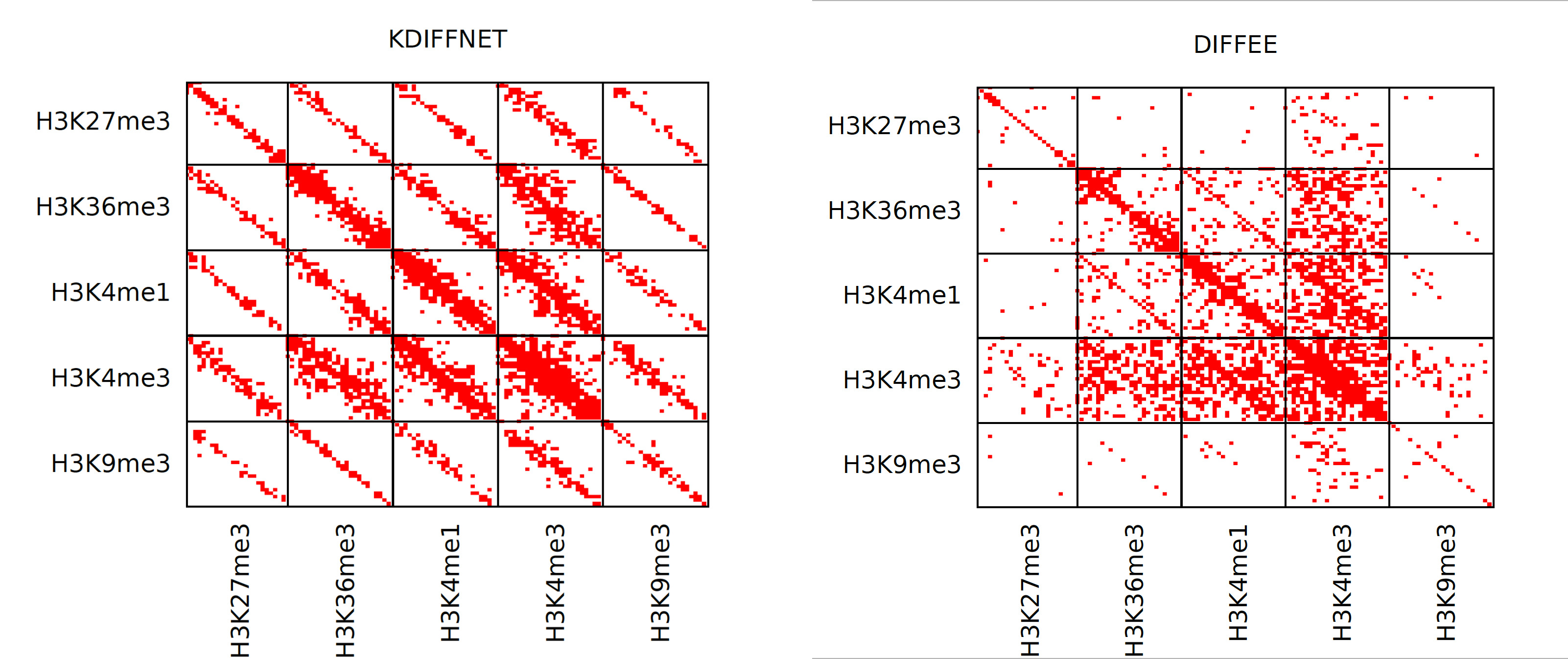
Figure 5: Epigenomic Dataset: Learnt Epigenetic Network represented as heatmaps: KDiffNet can discover biologically consistent interactions alongwith incorporating spatial information.

Table 4 shows the time cost of KDiffNet-E and baselines of estimating epigenetic network for cell type E123.

Method	E123	E116	E100
KDiffNet-E	0.8161$\pm$0.044	0.8161$\pm$0.032	0.7909$\pm$0.0299
DIFFEE	0.8073$\pm$0.050	0.8132$\pm$0.038	0.7879$\pm$0.036
JEEK	0.8113$\pm$0.042	0.8140$\pm$0.036	0.7880$\pm$0.034

Table 3: KDiffNet achieves highest Test Accuracy (averaged over $3$ splits) and standard deviation for three cell types E123, E116 and E003.

Method	E123	E116	E100
KDiffNet-E	0.002($\pm$ 0.000)	0.002($\pm$0.001)	0.001($\pm$ 0.000)
DIFFEE	0.001($\pm$ 0.000)	0.001($\pm$0.000)	0.001($\pm$ 0.000)
JEEK	3.004($\pm$0.092)	3.116($\pm$0.0646)	3.409 ($\pm$ 0.227)

Table 4: Average time cost(seconds) averaged over three data splits and standard deviation for three cell types E123, E116 and E003.

L.2 Experiment 4: Differential Genetic Network Identification from Gene Expression using SARS-CoV-2 and related datasets

Genes interact with each other for cellular signaling and regulatory processes. Discovering these interactions is important for identifying causal maps of molecular interactions as well as for using networks as bio markers. Section B.1 reviews data driven literature of extracting genetic networks and differential network identification from gene expression data. Complex diseases like the recent pandemic COVID-19 are the result of interactions between viruses and human (host) genes as well as interactions amongst human genes. The invading of the host by the virus perturbs the host’s gene expression and leads to rewiring mechanisms, consequentially gaining and losing interactions(Dimitrov, 2004). Understanding and identifying these changes following viral infection in the host genetic network is essential for the development of antiviral therapies.

Human Respiratory Viruses (including SARS-CoV-2) vs Control Dataset: In this experiment, we use the gene expression dataset measured across $\sim 20k$ from Blanco-Melo et al. (2020). This dataset measures the transcriptional response from the SARS-CoV-2 virus. Samples from primary human lung epithelium (NHBE) mock treated with SARS-CoV-2, IAV, a IAV that lacks the NS1 protein (IAVdNS1) and treated with human interferon-beta were collected. It also includes samples measured from lung alveolar (A549) cells and RSV or IAV transformed lung-derived Calu-3 cells infected with SARS-CoV-2. Additionally, uninfected human lung biopsies were also derived from two human subjects and a single male COVID-19 deceased patient.

Mouse Respiratory Virus vs Control Dataset: We use another similar dataset regarding viral respiratory infections from Xiong et al. (2014). This dataset includes gene expression measurements collected from mice with 2 or 4 days post viral infection whose lungs were used for total RNA-Seq. This dataset contains samples infected with multiple respiratory viruses and corresponding mock conditions. We aim to learn the differential graph between the virus infected samples($n_{d}=32$) and the control mock samples($n_{c}=88$). Similar to the previous case, we use the STRING database and DAVID databases for edge and group knowledge. We follow the same classification procedure as mentioned in the aforementioned case. Figure 6(b) shows the obtained classification performance.

Hyperparameters and evaluation pipeline

: To evaluate the different methods, we use a pairwise linear classification setting. In detail, we use the quadratic features from the estimated differential non-zero edges to classify a virus infected sample from a control sample. For every $(i,j)$ in the estimated graph, we use $x_{i}*x_{j}$ as a feature in a linear classification setting with elastic penalty. For all methods, we validate over $\lambda_{n}$ values that vary the fraction of zero edges(non-edges) of the inferred graphs from $0.01\times i|i\in\{50,51,52,\dots,98\}$. These features are fed to a logistic regressor with ridge penalty, which is trained via cross-validation on the train set. Finally, we report the accuracy on the test set. We use leave-three-out validation and hence, choose the best hyperparameters using the average validation set performance.

Our objective is to learn a differential graph between the virus infected condition and the control condition. For this purpose, we use the virus infected data samples as one class($n_{d}=38$) and the uninfected mock samples are used as the control samples($n_{c}=25$). Due to the lower number of samples in the dataset, we choose the top ranked $100$ genes with the highest variance in the log of rpkm gene expression counts. In Figure 7, we show the variance of the log of the gene expression in rpkm. Thus, our final number of features $p=100$.

For group level knowledge, we use group evidence from DAVID(Dennis et al., 2003) using their gene functional classification. To incorporate information regarding known interactions, we use the STRING(Szklarczyk et al., 2019) database. To account for the few number of samples, for our backward mapping, we use POET(Fan et al., 2013) as an estimation of an invertible covariance matrix.

Results:

Our classification results are shown in Figure 6(a). This pairwise classification strategy also helps to deal with model misspecification issues, as validation performance is an indicator of whether additional knowledge can be useful for estimation. This pairwise classification strategy also helps to deal with model misspecification issues, as validation performance is an indicator of whether additional knowledge can be useful for estimation.

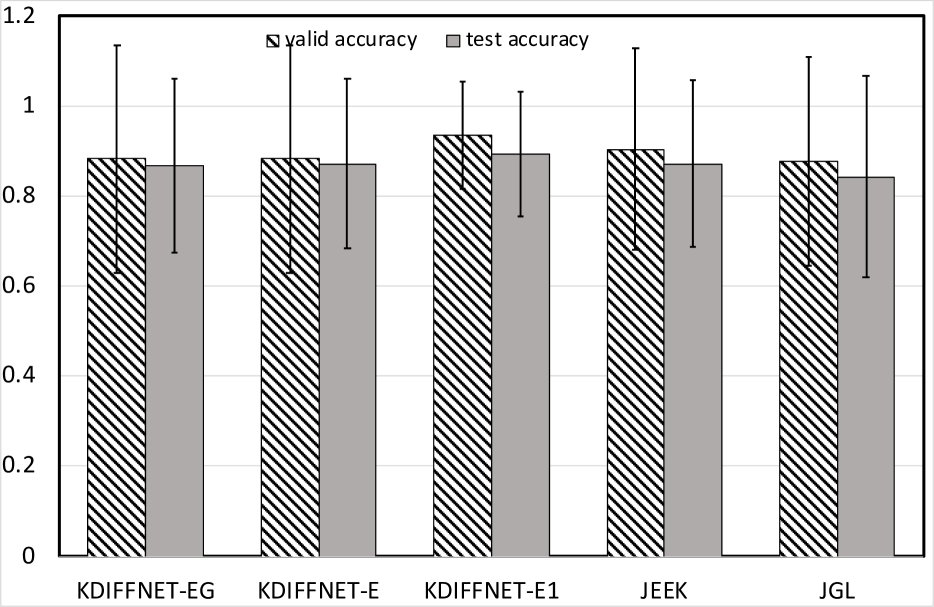
(a)

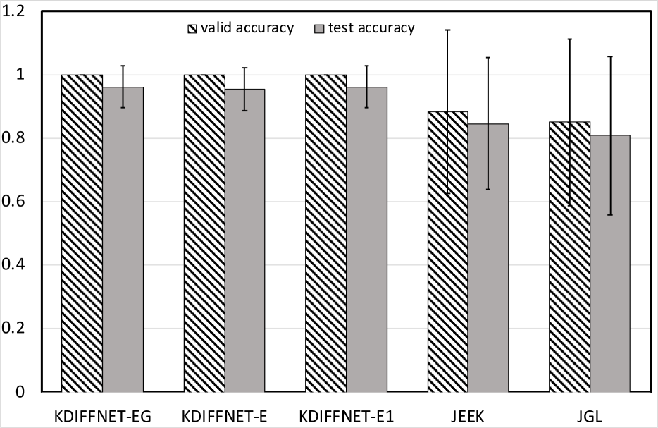
(b)

Figure 6: Validation and Test Accuracy on gene expression datasets : (a) Human Respiratory Viruses (including SARS-CoV-2) and (b) Mice Respiratory Viruses .

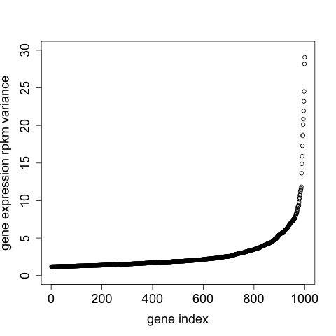
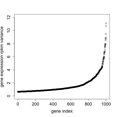
Figure 7: Variance of gene expression measurements(log of rpkm values). We show the top ranked $1000$ genes: (LEFT) For Human Respiratory Viruses and (RIGHT) For Mouse Respiratory Viruses Dataset.

Appendix M MORE DETAILS ON SIMULATED DATA

We use simulation to evaluate KDiffNet for improving differential structure estimation by making use of extra knowledge. In the following subsections, we present details about the data generation, followed by the results under multiple settings.

M.1 Simulation Dataset Generation

We generate simulated datasets with a clear underlying differential structure between two conditions, using the following method:

Data Generation for Edge Knowledge (KE):

Given a known weight matrix $W_{E}$ (e.g., spatial distance matrix between $p$ brain regions), we set $W^{d}=inv.logit(-W_{E})$. We use the assumption that higher the value of $W_{ij}$, lower the probability of that edge to occur in the true precision matrix. This is motivated by the role of spatial distance in brain connectivity networks: farther regions are less likely to be connected and vice-versa. We select different levels in the matrix $W^{d}$, denoted by $s$, where if $W^{d}_{ij}>s_{l}$, $\Delta^{d}_{ij}=0.5$, else $\Delta^{d}_{ij}=0$, where $\Delta^{d}\in{{\mathbb{R}}}^{p\times p}$. We denote by $s$ as the sparsity, i.e. the number of non-zero entries in $\Delta^{d}$. ${B}_{I}$ is a random graph with each edge ${B}_{{I}_{ij}}=0.5$ with probability $p$. $\delta_{c}$ and $\delta_{d}$ are selected large enough to guarantee positive definiteness.

$${\Omega}_{d}=\Delta^{d}+{B}_{I}+\delta_{d}I$$ (M.1)

$${\Omega}_{c}={B}_{I}+\delta_{c}I$$ (M.2)

$${\Delta}={\Omega}_{d}-{\Omega}_{c}$$ (M.3)

There is a clear differential structure in ${\Delta}={\Omega}_{d}-{\Omega}_{c}$, controlled by $\Delta^{d}$. To generate data from two conditions that follows the above differential structure, we generate two blocks of data samples following Gaussian distribution using $N(0,{\Omega}_{c}^{-1})$ and $N(0,{\Omega}_{d}^{-1})$. We only use these data samples to approximate the differential GGM to compare to the ground truth ${\Delta}$.

Data Generation for Vertex Knowledge (KG):

In this case, we simulate the case of extra knowledge of nodes in known groups. Let the node group size,i.e., the number of nodes with a similar interaction pattern in the differential graph be $m$. We select the block diagonals of size $m$ as groups in $\Delta^{g}$. If two variables $i,j$ are in a group $g^{\prime}$, in $\Delta^{g}_{ij}=0.5$, else $\Delta^{g}_{ij}=0$, where $\Delta^{g}\in{\mathbb{R}}^{p\times p}$. We denote by $s_{G}$ as the number of groups in $\Delta^{g}$. ${B}_{I}$ is a random graph with each edge ${B}_{{I}_{ij}}=0.5$ with probability $p$.

$${\Omega}_{d}=\Delta^{g}+{B}_{I}+\delta_{d}I$$ (M.4)

$${\Omega}_{c}={B}_{I}+\delta_{c}I$$ (M.5)

$${\Delta}={\Omega}_{d}-{\Omega}_{c}$$ (M.6)

$\delta_{c}$ and $\delta_{d}$ are selected large enough to guarantee positive definiteness. We generate two blocks of data samples following Gaussian distribution using $N(0,{\Omega}_{c}^{-1})$ and $N(0,{\Omega}_{d}^{-1})$.

Data Generation for both Edge and Vertex Knowledge (KEG):

In this case, we simulate the case of overlapping group and edge knowledge. Let the node group size,i.e., the number of nodes with a similar interaction pattern in the differential graph be $m$. We select the block diagonals of size $m$ as groups in $\Delta^{g}$. If two variables $i,j$ are in a group $g^{\prime}$, in $\Delta^{g}_{ij}=1/3$, else $\Delta^{g}_{ij}=0$, where $\Delta^{g}\in{\mathbb{R}}^{p\times p}$.

For the edge-level knowledge component, given a known weight matrix $W_{E}$, we set $W^{d}=inv.logit(-W_{E})$. Higher the value of $W_{E_{ij}}$, lower the value of $W^{d}_{ij}$, hence lower the probability of that edge to occur in the true precision matrix. We select different levels in the matrix $W^{d}$, denoted by $s$, where if $W^{d}_{ij}>s_{l}$, we set $\Delta^{d}_{ij}=1/3$, else $\Delta^{d}_{ij}=0$. We denote by $s$ as the number of non-zero entries in $\Delta^{d}$. ${B}_{I}$ is a random graph with each edge ${B}_{{I}_{ij}}=1/3$ with probability $p$.

$${\Omega}_{d}=\Delta^{d}+\Delta^{g}+{B}_{I}+\delta_{d}I$$ (M.7)

$${\Omega}_{c}={B}_{I}+\delta_{c}I$$ (M.8)

$${\Delta}={\Omega}_{d}-{\Omega}_{c}$$ (M.9)

$\delta_{c}$ and $\delta_{d}$ are selected large enough to guarantee positive definiteness. Similar to the previous case, we generate two blocks of data samples following Gaussian distribution using $N(0,{\Omega}_{c}^{-1})$ and $N(0,{\Omega}_{d}^{-1})$. We only use these data samples to approximate the differential GGM to compare to the ground truth ${\Delta}$.

We consider three different types of known edge knowledge $W_{E}$ generated from the spatial distance between different brain regions and simulate groups to represent related anatomical regions. These three are distinguished by different $p=\{116,160,246\}$ representing spatially related brain regions. We generate three types of datasets:Data-EG (having both edge and vertex knowledge), Data-G(with edge-level extra knowledge) and Data-V(with known node groups knowledge). We generate two blocks of data samples $\bm{X}_{c}$ and $\bm{X}_{d}$ following Gaussian distribution using $N(0,{\Omega}_{c}^{-1})$ and $N(0,{\Omega}_{d}^{-1})$. We use these data samples to estimate the differential GGM to compare to the ground truth ${\Delta}$. We vary the sparsity of the true differential graph ($s$) and the number of control and case samples ($n_{c}$ and $n_{d}$ respectively) used to estimate the differential graph. For each case of $p$, we vary $n_{c}$ and $n_{d}$ in $\{p/2,p/4,p,2p\}$ to account for both high dimensional and low dimensional cases. The sparsity of the underlying differential graph is controlled by $s=\{0.125,0.25,0.375,0.5\}$ and $s_{G}$ as explained above. This results in $126$ different datasets representing diverse settings: different number of dimensions $p$, number of samples $n_{c}$ and $n_{d}$, multiple levels of sparsity $s$ and number of groups $s_{G}$ of the differential graph for both KE and KEG data settings. Figure 8 summarizes the different settings for simulation datasets.

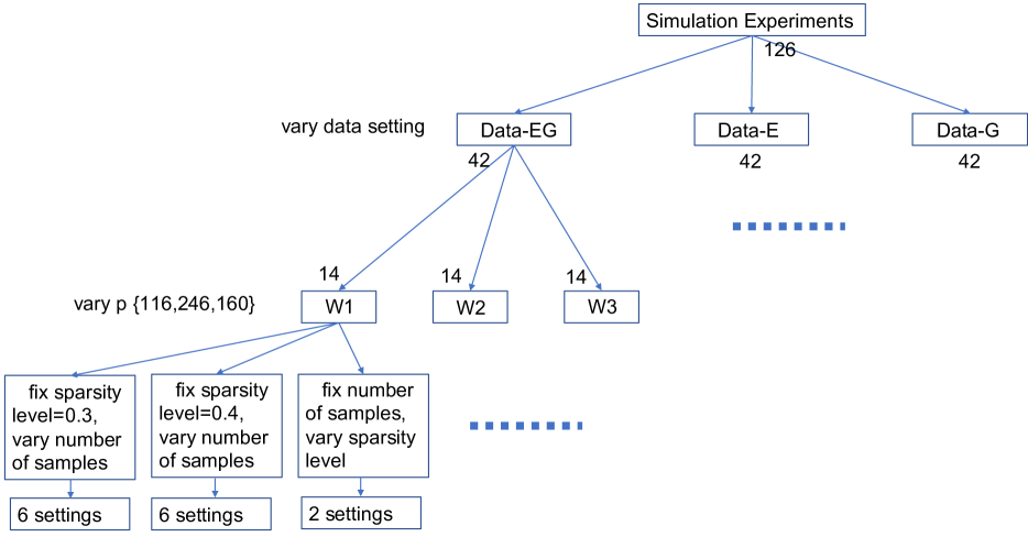
Figure 8: A schematic showing the different experimental settings for simulation experiments.

Experiment Design: We consider three different types of known edge knowledge $W_{E}$ generated from the spatial distance between different brain regions and simulate groups to represent related anatomical regions. These three are distinguished by different $p=\{116,160,246\}$ representing spatially related brain regions. We vary $n_{c}$ and $n_{d}$ in $\{p/2,p/4,p,2p\}$ to account for both high dimensional and low dimensional cases. The sparsity of the underlying differential graph is controlled by $s=\{0.125,0.25,0.375,0.5\}$ and $s_{G}$. This results in $126$ different datasets representing diverse settings: multiple $p$, number of samples $n_{c}$ and $n_{d}$, sparsity $s$ and number of groups $s_{G}$ of the differential graph for both KE and KEG data settings.

Appendix N MORE ANALYSIS AND DETAILS ON RESULTS ON SIMULATED DATASETS:

N.1 Simulated Results: When we compare with Deep Neural Network based models(GNN)

W2	level	samples	hidden	layers	GAT F1 Score	KDiffNet-EG F1 Score
246	4	61	64	1	0.0054	0.9384
246	4	123	64	3	0.0102	0.9397
246	4	246	32	2	0.0095	0.9365
246	4	492	64	1	0.0205	0.9430
246	5	61	5	3	0.0114	0.9225
246	5	123	64	1	0.0136	0.9219
246	5	246	32	3	0.0231	0.9248
246	5	492	16	2	0.0740	0.9302

Table 5: Comparison of KDiffNet-EG and GATVeličković et al. (2017) for differential graph recovery.

We compare with Graph Attention Networks(Veličković et al., 2017). Although not designed for differential parameter learning, we explore the graphs learnt by the attention weights in relation to the true differential graph. We formulate it as a classification task, that is each distribution represents a labeled class. In detail, for each sample, we predict the corresponding data block $\in\{c,d\}$. We validate over number of layers $\in\{1,2,3,4,5\}$ and hidden size $\{5,16,32,64\}$ for $W2$, $p=246$ and varying samples in $\{61,123,246,492\}$ for train,validation and test sets in each setting. We use one attention head in this setting. We train the models using ADAM optimizer with learning rate $0.0005$ and train each model for $300$ epochs. We pick the model based on the epoch with best validation set classification performance. We use the training set samples to select a threshold for binarizing the aggregated difference of attention weights across the samples from the two data blocks(classes). We report the F1-Score on the aggregated difference from the classes using attention weights from the test data samples. Table 5 shows the GAT performance and corresponding KDiffNet-EG performance for the different settings.

We adapt a recently proposed deep learning based neighborhood selection method to estimate network structure(Ke et al., 2019). We use the setting as proposed for a single task from Sekhon et al. (2020). We compare to the simulation case with samples $n_{c}=n_{d}\in\{p,2p\}$ and $p=\{116,246,160\}$ with sparsity level $5$. We use the same datasets as used in the simulation experiments. We use an MLP layer of size $4\times p$. We show the results in Table 6. We validate over sparsity regularization $\lambda_{n}\in\{1e-03,1e-04,1e-05\}$. In such high dimensional cases, MLP based deep models are not able to learn the correct differential structures, as indicated by lower edge level F1 score.

Method	W1	W2	W3
KDiffNet	0.74/0.74	0.92/0.93	0.94/0.94
DL	0.54/0.55	0.54/0.54	0.56/0.56

Table 6: Edge Recovery Accuracy of KDiffNet vs deep learning(DL) based neighborhood selection methods for $n_{c}=n_{d}\in\{p,2p\}$.

N.2 Simulated Results: when our knowledge is partial

Varying proportion of known edges:

We generate $W_{E}$ matrices with $p=150$ using Erdos Renyi Graph (ErdHos and Rényi, 1960). We use the generated graph as prior edge knowledge $W_{E}$. Additionally, we simulate $15$ groups of size $10$ as explained in  Section M.1. We simulate $\Omega_{c}$ and $\Omega_{d}$ as explained in  Section M.1. Figure 9 presents the performance of KDiffNet-EG , KDiffNet-E and DIFFEE with varying proportion of known edges.

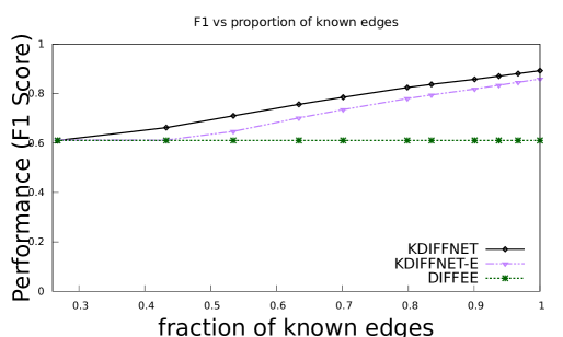
Figure 9: F1-Score of KDiffNet-EG ,KDiffNet-E and DIFFEE with varying proportion of known edges.

KDiffNet-EG has a higher F1-score than KDiffNet-E as it can additionally incorporate known group information. As expected, with increase in the proportion of known edges, F1-Score improves for both KDiffNet-EG and KDiffNet-E . In contrast DIFFEE cannot make use of additional information and the F1-Score remains the same.

N.3 Simulated Results: When Tuning hyperparameters and Varying $p$

Scalability in $p$:

To evaluate the scalability of KDiffNet and baselines to large $p$, we also generate larger $W_{E}$ matrices with $p=2000$ using Erdos Renyi Graph ErdHos and Rényi (1960), similar to the aforementioned design. Using the generated graph as prior edge knowledge $W_{E}$, we design $\Omega_{c}$ and $\Omega_{d}$ as explained in  Section M.1. For the case of both edge and vertex knowledge, we fix the number of groups to $100$ of size $10$. We evaluate the scalability of KDiffNet-EG and baselines measured in terms of computation cost per $\lambda_{n}$.

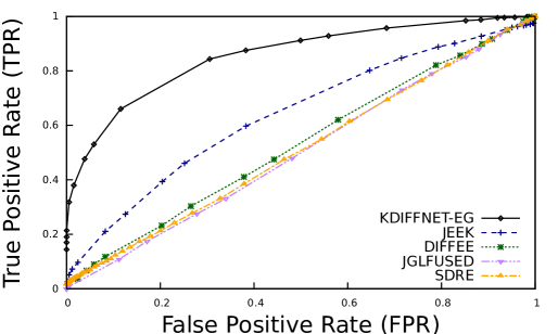
Figure 10: Area Under Curve (AUC) Curves for KDiffNet and baselines at different hyperparameter values $\lambda$.

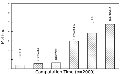
Figure 11: Scalability of KDiffNet : Computation Time (log milliseconds) per $\lambda_{n}$ for large $p=2000$: KDiffNet-EG has reasonable time cost with respect to baseline methods. KDiffNet-E and KDiffNet-G are fast due to closed form.

Figure 11 shows the computation time cost per $\lambda_{n}$ for all methods. Clearly, KDiffNet takes the least time, for very large $p$ as well.

Choice of $\lambda_{n}$:

For KDiffNet , we show the performance of all the methods as a function of choice of $\lambda_{n}$. Figure 10 shows the True Positive Rate(TPR) and False Positive Rate(FPR) measured by varying $\lambda_{n}$ for $p=116$, $s=0.5$ and $n_{c}=n_{d}=p/2$ under the Data-EG setting. Clearly, KDiffNet-EG achieves the highest Area under Curve (AUC) than all other baseline methods. KDiffNet-EG also outperforms JEEK and NAK that take into account edge knowledge but cannot model the known group knowledge.

N.4 Simulated Results: When we have both edge and group knowledge:

Edge and Vertex Knowledge (KEG):

We use KDiffNet (Algorithm 1) to infer the differential structure in this case.

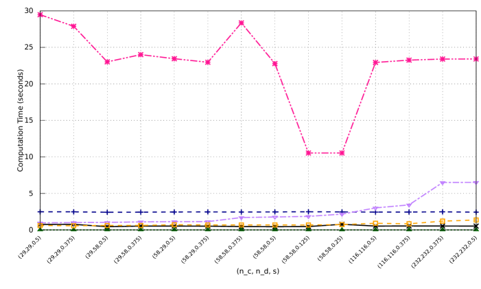
Figure 12: KDiffNet Edge and Vertex Knowledge Simulation Results for $p=116$ for different settings of $n_{c},n_{d}$ and $s$: (a) The test F1-score and (b) The average computation time (measured in seconds) per $\lambda_{n}$ for KDiffNet and baseline methods.

Figure 12(a) shows the performance in terms of F1 Score of KDiffNet in comparison to the baselines for $p=116$, corresponding to 116 regions of the brain. KDiffNet outperforms the best baseline in each case by an average improvement of $~{}414\%$. KDiffNet-EG does better than JEEK and NAK that can model the edge information but cannot include group information. SDRE and DIFFEE are direct estimators but perform poorly indicating that adding additional knowledge aids differential network estimation. JGLFUSED performs the worst on all cases.

Figure 12(b) shows the average computation cost per $\lambda_{n}$ of each method measured in seconds. In all settings, KDiffNet has lower computation cost than JEEK, SDRE and JGLFUSED in different cases of varying $n_{c}$ and $n_{d}$, as well as with different sparsity of the differential network. KDiffNet is on average $~{}24\times$ faster than the best performing baseline. It is slower than DIFFEE owing to DIFFEE’s non-iterative closed form solution, however, DIFFEE does not have good prediction performance. Note that $B^{*}()$ in KDiffNet , JEEK and DIFFEE and the kernel term in SDRE are precomputed only once prior to tuning across multiple $\lambda_{n}$.

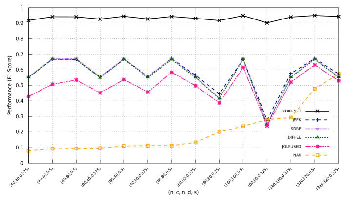
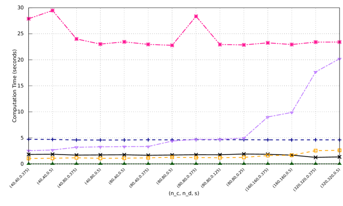
Figure 13: KDiffNet Edge and Vertex Knowledge Simulation Results for $p=160$ for different settings of $n_{c},n_{d}$ and $s$: (a) The test F1-score and (b) The average computation time (measured in seconds) per $\lambda_{n}$ for KDiffNet and baseline methods.

In Figure 13(a), we plot the test F1-score for simulated datasets generated using $W$ with $p=160$, representing spatial distances between different $160$ regions of the brain. This represents a larger and different set of spatial brain regions. In $p=160$ case, KDiffNet outperforms the best baseline in each case by an average improvement of $~{}928\%$. Including available additional knowledge is clearly useful as JEEK does relatively better than the other baselines. JGLFUSED performs the worst on all cases. Figure 13(b) shows the computation cost of each method measured in seconds for each case. KDiffNet is on average $~{}37\times$ faster than the best performing baseline.

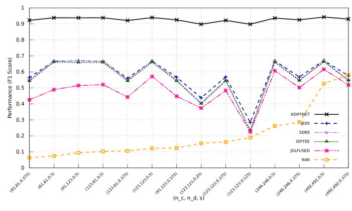
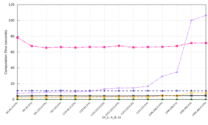
Figure 14: KDiffNet Edge and Vertex Knowledge Simulation Results for $p=246$ for different settings of $n_{c},n_{d}$ and $s$: (a) The test F1-score and (b) The average computation time (measured in seconds) per $\lambda_{n}$ for KDiffNet and baseline methods

In Figure 14(a), we plot the test F1-score for simulated datasets generated using a larger $W_{E}$ with $p=246$, representing spatial distances between different $246$ regions of the brain. This represents a larger and different set of spatial brain regions. In this case, KDiffNet outperforms the best baseline in each case by an average improvement of $1400\%$ relative to the best performing baseline. In this case as well, including available additional knowledge is clearly useful as JEEK does relatively better than the other baselines, which do not incorporate available additional knowledge. JGLFUSED again performs the worst on all cases. Figure 14(b) shows the computation cost of each method measured in seconds for each case. In all cases, KDiffNet has the least computation cost in different settings of the data generation. KDiffNet is on average $~{}20\times$ faster than the best performing baseline.

We cannot compare Diff-CLIME as it takes more than  2 days to finish $p=246$ case.

N.5 Simulated Results: When we have only edge knowledge:

Edge Knowledge (KE):

Given known $W_{E}$, we use KDiffNet-E to infer the differential structure in this case.

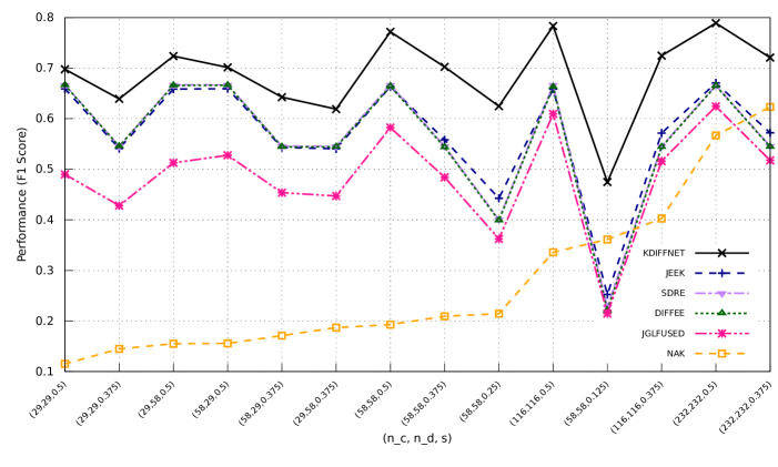
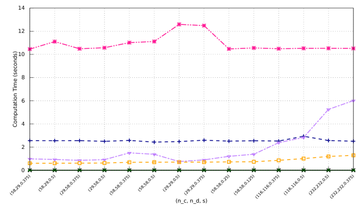
Figure 15: KDiffNet-E Simulation Results for $p=116$ for different settings of $n_{c},n_{d}$ and $s$: (a) The test F1-score and (b) The average computation time (measured in seconds) per $\lambda_{n}$ for KDiffNet-E and baseline methods.

Figure 15(a) shows the performance in terms of F1-Score of KDiffNet-E in comparison to the baselines for $p=116$, corresponding to 116 spatial regions of the brain. In $p=116$ case, KDiffNet-E outperforms the best baseline in each case by an average improvement of $23\%$. While JEEK, DIFFEE and SDRE perform similar to each other, JGLFUSED performs the worst on all cases.

Figure 15(b) shows the computation cost of each method measured in seconds for each case. In all cases, KDiffNet-E has the least computation cost in different cases of varying $n_{c}$ and $n_{d}$, as well as with different sparsity of the differential network. For $p=116$, KDiffNet-E , owing to an entry wise parallelizable closed form solution, is on average $~{}2356\times$ faster than the best performing baseline.

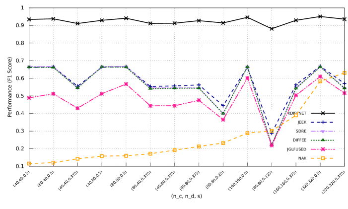
Figure 16: KDiffNet-E Simulation Results for $p=160$ for different settings of $n_{c},n_{d}$ and $s$: (a) The test F1-score and (b) The average computation time (measured in seconds) per $\lambda_{n}$ for KDiffNet-E and baseline methods.

In Figure 16(a), we plot the test F1-score for simulated datasets generated using $W$ with $p=160$, representing spatial distances between different $160$ regions of the brain. This represents a larger and different set of spatial brain regions. In $p=160$ case, KDiffNet-E outperforms the best baseline in each case by an average improvement of $67.5\%$. Including available additional knowledge is clearly useful as JEEK does relatively better than the other baselines, which do not incorporate available additional knowledge. JGLFUSED performs the worst on all cases. Figure 16(b) shows the computation cost of each method measured in seconds for each case. In all cases, KDiffNet-E has the least computation cost in different cases of varying $n_{c}$ and $n_{d}$, as well as with different sparsity of the differential network. KDiffNet-E is on average $~{}3300\times$ faster than the best performing baseline.

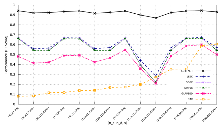
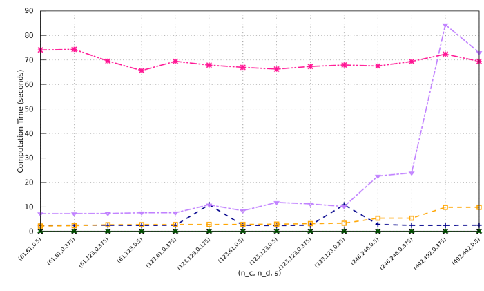
Figure 17: KDiffNet-E Simulation Results for $p=246$ for different settings of $n_{c},n_{d}$ and $s$: (a) The test F1-score and (b) The average computation time (measured in seconds) per $\lambda_{n}$ for KDiffNet-E and baseline methods.

In Figure 17(a), we plot the test F1-score for simulated datasets generated using a larger $W$ with $p=246$, representing spatial distances between different $246$ regions of the brain. This represents a larger and different set of spatial brain regions. In this case, KDiffNet-E outperforms the best baseline in each case by an average improvement of $66.4\%$ relative to the best performing baseline. Including available additional knowledge is clearly useful as JEEK does relatively better than the other baselines, which do not incorporate available additional knowledge. JGLFUSED performs the worst on all cases. Figure 17(b) shows the computation cost of each method measured in seconds for each case. In all cases, KDiffNet-E has the least computation cost in different cases of varying $n_{c}$ and $n_{d}$, as well as with different sparsity of the differential network. KDiffNet-E is on average $~{}3966\times$ faster than the best performing baseline.

N.6 Simulated Results: When we have only group knowledge:

Node Group Knowledge

: We use KDiffNet-G to estimate the differential network with the known groups as extra knowledge. We vary the number of groups $s_{G}$ and the number of samples $n_{c}$ and $n_{d}$ for each case of $p=\{116,160,246\}$. Figure 18 shows the F1-Score of KDiffNet-G and the baselines for $p=116$. KDiffNet-G clearly has a large advantage when extra node group knowledge is available. The baselines cannot model such available knowledge.

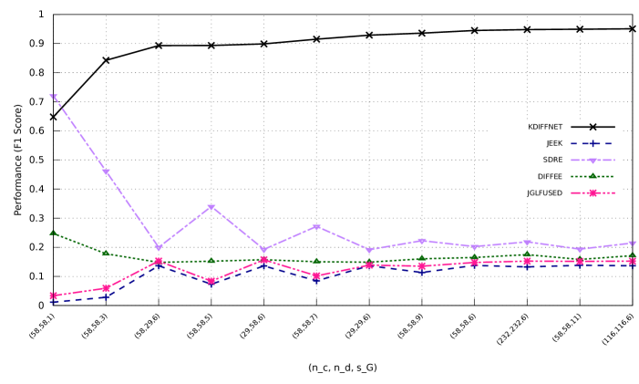
Figure 18: KDiffNet-G Simulation Results for $p=246$ for different settings of $n_{c},n_{d}$ and $s$: (a) The test F1-score and (b) The average computation time (measured in seconds) per $\lambda_{n}$ for KDiffNet-E and baseline methods.

N.7 Knowledge of Perturbed Hub nodes

We consider the case where there exists a set of nodes $k\in P$ such that the group of edges defined by $\Omega_{c_{k,j}}=0$ and $\Omega_{d_{k,j}}\neq 0$, where $\forall j\in\{1,\dots,p\},k\in P$. Here, P denotes the set of perturbed nodes.

To generate the simulation data, $\Delta{{k,j}}=1.0$ where $\forall j\in\{1,\dots,p\},k\in P$. ${\Omega}_{d}=\Delta+{B}_{I}+\delta_{d}I$, ${\Omega}_{c}={B}_{I}+\delta_{c}I$, finally, ${\Delta}={\Omega}_{d}-{\Omega}_{c}$. $\delta_{c}$ and $\delta_{d}$ are selected large enough to guarantee positive definiteness. We generate two blocks of data samples following Gaussian distribution using $N(0,{\Omega}_{c}^{-1})$ and $N(0,{\Omega}_{d}^{-1})$.

We report our results in Figure 2(c). We compare KDiffNet-G , KDiffNet-E , JEEK, DIFFEE, and JGL-perturb. KDiffNet-G directly takes into account the perturbed groups, by imposing a group penalty on the relevant edges. For KDiffNet-E and JEEK, we set $W_{k,j}=0.1$.

References

• Allen and Liu (2013) Genevera I Allen and Zhandong Liu. A local poisson graphical model for inferring networks from sequencing data. IEEE transactions on nanobioscience, 12(3):189–198, 2013.
• Belilovsky et al. (2016) Eugene Belilovsky, Gaël Varoquaux, and Matthew B Blaschko. Testing for differences in gaussian graphical models: applications to brain connectivity. In Advances in Neural Information Processing Systems, pages 595–603, 2016.
• Berger (2007) Shelley L Berger. The complex language of chromatin regulation during transcription. Nature, 447(7143):407–412, 2007.
• Bickel and Levina (2008) Peter J Bickel and Elizaveta Levina. Covariance regularization by thresholding. The Annals of Statistics, pages 2577–2604, 2008.
• Blanco-Melo et al. (2020) Daniel Blanco-Melo, Benjamin Nilsson-Payant, Wen-Chun Liu, Rasmus Møller, Maryline Panis, David Sachs, Randy Albrecht, et al. Sars-cov-2 launches a unique transcriptional signature from in vitro, ex vivo, and in vivo systems. BioRxiv, 2020.
• Bu and Lederer (2017) Yunqi Bu and Johannes Lederer. Integrating additional knowledge into estimation of graphical models. arXiv preprint arXiv:1704.02739, 2017.
• Combettes and Pesquet (2011) Patrick L Combettes and Jean-Christophe Pesquet. Proximal splitting methods in signal processing. In Fixed-point algorithms for inverse problems in science and engineering, pages 185–212. Springer, 2011.
• Craddock et al. (2013) C Craddock, S Sikka, B Cheung, R Khanuja, SS Ghosh, C Yan, Q Li, D Lurie, J Vogelstein, R Burns, et al. Towards automated analysis of connectomes: The configurable pipeline for the analysis of connectomes. Front Neuroinform, 42, 2013.
• Craddock (2014) Cameron Craddock. Preprocessed connectomes project: open sharing of preprocessed neuroimaging data and derivatives. In 61st Annual Meeting. AACAP, 2014.
• Da Wei Huang and Lempicki (2008) Brad T Sherman Da Wei Huang and Richard A Lempicki. Systematic and integrative analysis of large gene lists using DAVID bioinformatics resources. Nature protocols, 4(1):44–57, 2008.
• Danaher et al. (2013) Patrick Danaher, Pei Wang, and Daniela M Witten. The joint graphical lasso for inverse covariance estimation across multiple classes. Journal of the Royal Statistical Society: Series B (Statistical Methodology), 2013.
• de la Fuente (2010) Alberto de la Fuente. From ‘differential expression’to ‘differential networking’–identification of dysfunctional regulatory networks in diseases. Trends in genetics, 26(7):326–333, 2010.
• Dennis et al. (2003) Glynn Dennis, Brad T Sherman, Douglas A Hosack, Jun Yang, Wei Gao, H Clifford Lane, and Richard A Lempicki. David: database for annotation, visualization, and integrated discovery. Genome biology, 4(9):R60, 2003.
• Di Martino et al. (2014) Adriana Di Martino, Chao-Gan Yan, Qingyang Li, Erin Denio, Francisco X Castellanos, Kaat Alaerts, Jeffrey S Anderson, Michal Assaf, Susan Y Bookheimer, Mirella Dapretto, et al. The autism brain imaging data exchange: towards a large-scale evaluation of the intrinsic brain architecture in autism. Molecular psychiatry, 19(6):659–667, 2014.
• Dimitrov (2004) Dimiter S Dimitrov. Virus entry: molecular mechanisms and biomedical applications. Nature Reviews Microbiology, 2(2):109–122, 2004.
• Dobra et al. (2004) Adrian Dobra, Chris Hans, Beatrix Jones, Joseph R Nevins, Guang Yao, and Mike West. Sparse graphical models for exploring gene expression data. Journal of Multivariate Analysis, 90(1):196–212, 2004.
• Dong et al. (2012) Xianjun Dong, Melissa C Greven, Anshul Kundaje, Sarah Djebali, James B Brown, Chao Cheng, Thomas R Gingeras, Mark Gerstein, Roderic Guigó, Ewan Birney, et al. Modeling gene expression using chromatin features in various cellular contexts. Genome biology, 13(9):R53, 2012.
• Dosenbach et al. (2010) Nico UF Dosenbach, Binyam Nardos, Alexander L Cohen, Damien A Fair, Jonathan D Power, Jessica A Church, Steven M Nelson, Gagan S Wig, Alecia C Vogel, Christina N Lessov-Schlaggar, et al. Prediction of individual brain maturity using fmri. Science, 329(5997):1358–1361, 2010.
• ErdHos and Rényi (1960) Paul ErdHos and Alfréd Rényi. On the evolution of random graphs. Publ. Math. Inst. Hung. Acad. Sci, 5(1):17–60, 1960.
• (20) Jianqing Fan and Han Liu. Statistical analysis of big data on pharmacogenomics. 65(7):987–1000.
• Fan et al. (2013) Jianqing Fan, Yuan Liao, and Martina Mincheva. Large covariance estimation by thresholding principal orthogonal complements. Journal of the Royal Statistical Society: Series B (Statistical Methodology), 75(4):603–680, 2013.
• Fazayeli and Banerjee (2016) Farideh Fazayeli and Arindam Banerjee. Generalized direct change estimation in ising model structure. In International Conference on Machine Learning, pages 2281–2290, 2016.
• Haury et al. (2012) Anne-Claire Haury, Fantine Mordelet, Paola Vera-Licona, and Jean-Philippe Vert. Tigress: trustful inference of gene regulation using stability selection. BMC systems biology, 6(1):145, 2012.
• Honorio and Samaras (2010) Jean Honorio and Dimitris Samaras. Multi-task learning of gaussian graphical models. In Proceedings of the 27th International Conference on Machine Learning (ICML-10), page 447, 2010.
• Ideker and Krogan (2012) Trey Ideker and Nevan J Krogan. Differential network biology. Molecular systems biology, 8(1):565, 2012.
• Ke et al. (2019) Nan Rosemary Ke, Olexa Bilaniuk, Anirudh Goyal, Stefan Bauer, Hugo Larochelle, Bernhard Schölkopf, Michael C Mozer, Chris Pal, and Yoshua Bengio. Learning neural causal models from unknown interventions. arXiv preprint arXiv:1910.01075, 2019.
• Kundaje et al. (2015) Anshul Kundaje, Wouter Meuleman, Jason Ernst, Misha Bilenky, Angela Yen, Alireza Heravi-Moussavi, Pouya Kheradpour, Zhizhuo Zhang, Jianrong Wang, Michael J Ziller, et al. Integrative analysis of 111 reference human epigenomes. Nature, 518(7539):317–330, 2015.
• Kyung et al. (2010) Minjung Kyung, Jeff Gill, Malay Ghosh, George Casella, et al. Penalized regression, standard errors, and bayesian lassos. Bayesian Analysis, 5(2):369–411, 2010.
• Liu et al. (2014) Song Liu, John A Quinn, Michael U Gutmann, Taiji Suzuki, and Masashi Sugiyama. Direct learning of sparse changes in markov networks by density ratio estimation. Neural computation, 26(6):1169–1197, 2014.
• Liu et al. (2017) Song Liu, Kenji Fukumizu, and Taiji Suzuki. Learning sparse structural changes in high-dimensional markov networks. Behaviormetrika, 44(1):265–286, 2017.
• Margolin et al. (2006) Adam A Margolin, Ilya Nemenman, Katia Basso, Chris Wiggins, Gustavo Stolovitzky, Riccardo Dalla Favera, and Andrea Califano. Aracne: an algorithm for the reconstruction of gene regulatory networks in a mammalian cellular context. In BMC bioinformatics, volume 7, page S7. Springer, 2006.
• Meinshausen and Bühlmann (2006) Nicolai Meinshausen and Peter Bühlmann. High-dimensional graphs and variable selection with the lasso. The annals of statistics, pages 1436–1462, 2006.
• Meyer et al. (2007) Patrick E Meyer, Kevin Kontos, Frederic Lafitte, and Gianluca Bontempi. Information-theoretic inference of large transcriptional regulatory networks. EURASIP journal on bioinformatics and systems biology, 2007:1–9, 2007.
• Mohan et al. (2014) Karthik Mohan, Maryam Fazel Palma London, Daniela Witten, and Su-In Lee. Node-based learning of multiple gaussian graphical models. JMLR, 15(1):445, 2014.
• Mukherjee and Speed (2008) Sach Mukherjee and Terence P Speed. Network inference using informative priors. Proceedings of the National Academy of Sciences, 105(38):14313–14318, 2008.
• Negahban et al. (2009) Sahand Negahban, Bin Yu, Martin J Wainwright, and Pradeep K Ravikumar. A unified framework for high-dimensional analysis of $m$-estimators with decomposable regularizers. In Advances in Neural Information Processing Systems, pages 1348–1356, 2009.
• (37) Ke Niu, Jiayang Guo, Yijie Pan, Xin Gao, Xueping Peng, Ning Li, and Hailong Li. Multichannel deep attention neural networks for the classification of autism spectrum disorder using neuroimaging and personal characteristic data. Complexity, 2020.
• Poldrack et al. (2013) Russell A Poldrack, Deanna M Barch, Jason Mitchell, Tor Wager, Anthony D Wagner, Joseph T Devlin, Chad Cumba, Oluwasanmi Koyejo, and Michael Milham. Toward open sharing of task-based fmri data: the openfmri project. Frontiers in neuroinformatics, 7:12, 2013.
• Prasad et al. (2009) TS Keshava Prasad, Renu Goel, Kumaran Kandasamy, Shivakumar Keerthikumar, Sameer Kumar, Suresh Mathivanan, Deepthi Telikicherla, Rajesh Raju, Beema Shafreen, Abhilash Venugopal, et al. Human protein reference database 2009 update. Nucleic acids research, 37(suppl 1):D767–D772, 2009.
• Ravikumar et al. (2011) Pradeep Ravikumar, Martin J Wainwright, Garvesh Raskutti, Bin Yu, et al. High-dimensional covariance estimation by minimizing l1-penalized log-determinant divergence. Electronic Journal of Statistics, 5:935–980, 2011.
• Rothman et al. (2009) Adam J Rothman, Elizaveta Levina, and Ji Zhu. Generalized thresholding of large covariance matrices. Journal of the American Statistical Association, 104(485):177–186, 2009.
• (42) Juliane Schäfer and Korbinian Strimmer. A shrinkage approach to large-scale covariance matrix estimation and implications for functional genomics. Statistical applications in genetics and molecular biology, 4(1).
• Sekhon et al. (2020) Arshdeep Sekhon, Zhe Wang, and Yanjun Qi. Relate and predict: Structure-aware prediction with jointly optimized neural dependency graph. 2020.
• Shimamura et al. (2007) Teppei Shimamura, Seiya Imoto, Rui Yamaguchi, and Satoru Miyano. Weighted lasso in graphical gaussian modeling for large gene network estimation based on microarray data. In Genome Informatics 2007: Genome Informatics Series Vol. 19, pages 142–153. World Scientific, 2007.
• Singh et al. (2017) Chandan Singh, Beilun Wang, and Yanjun Qi. A constrained, weighted-l1 minimization approach for joint discovery of heterogeneous neural connectivity graphs. arXiv preprint arXiv:1709.04090, 2017.
• Suganuma and Workman (2008) Tamaki Suganuma and Jerry L Workman. Crosstalk among histone modifications. Cell, 135(4):604–607, 2008.
• Szklarczyk et al. (2019) Damian Szklarczyk, Annika L Gable, David Lyon, et al. String v11: protein–protein association networks with increased coverage, supporting functional discovery in genome-wide experimental datasets. Nucleic acids research, 47(D1):D607–D613, 2019.
• Vân Anh Huynh-Thu et al. (2010) Alexandre Irrthum Vân Anh Huynh-Thu, Louis Wehenkel, and Pierre Geurts. Inferring regulatory networks from expression data using tree-based methods. PloS one, 5(9), 2010.
• Van Essen et al. (2013) David C Van Essen, Stephen M Smith, Deanna M Barch, Timothy EJ Behrens, Essa Yacoub, Kamil Ugurbil, WU-Minn HCP Consortium, et al. The wu-minn human connectome project: an overview. Neuroimage, 80:62–79, 2013.
• Veličković et al. (2017) Petar Veličković, Guillem Cucurull, Arantxa Casanova, Adriana Romero, Pietro Lio, and Yoshua Bengio. Graph attention networks. arXiv preprint arXiv:1710.10903, 2017.
• Vértes et al. (2012) Petra E Vértes, Aaron F Alexander-Bloch, Nitin Gogtay, Jay N Giedd, Judith L Rapoport, and Edward T Bullmore. Simple models of human brain functional networks. Proceedings of the National Academy of Sciences, 109(15):5868–5873, 2012.
• Wainwright and Jordan (2008) Martin J Wainwright and Michael I Jordan. Graphical models, exponential families, and variational inference. Foundations and Trends® in Machine Learning, 1(1-2):1–305, 2008.
• Wang et al. (2018a) Beilun Wang, Arshdeep Sekhon, and Yanjun Qi. A fast and scalable joint estimator for integrating additional knowledge in learning multiple related sparse gaussian graphical models. In International Conference on Machine Learning, pages 5161–5170, 2018a.
• Wang et al. (2018b) Beilun Wang, Arshdeep Sekhon, and Yanjun Qi. Fast and scalable learning of sparse changes in high-dimensional gaussian graphical model structure. In Proceedings of AISTATS, 2018b.
• Watts and Strogatz (1998) Duncan J Watts and Steven H Strogatz. Collective dynamics of ‘small-world’networks. nature, 393(6684):440, 1998.
• (56) Adriano V Werhli and Dirk Husmeier. Reconstructing gene regulatory networks with bayesian networks by combining expression data with multiple sources of prior knowledge. Statistical applications in genetics and molecular biology, 6(1).
• Xiong et al. (2014) Hao Xiong, Juliet Morrison, et al. Genomic profiling of collaborative cross founder mice infected with respiratory viruses reveals novel transcripts and infection-related strain-specific gene and isoform expression. G3: Genes, Genomes, Genetics, 4(8):1429–1444, 2014.
• Yang et al. (2014a) Eunho Yang, Aurélie C Lozano, and Pradeep Ravikumar. Elementary estimators for high-dimensional linear regression. In Proceedings of the 31st International Conference on Machine Learning (ICML-14), pages 388–396, 2014a.
• Yang et al. (2014b) Eunho Yang, Aurélie C Lozano, and Pradeep D Ravikumar. Elementary estimators for sparse covariance matrices and other structured moments. In ICML, pages 397–405, 2014b.
• Yang et al. (2014c) Eunho Yang, Aurélie C Lozano, and Pradeep K Ravikumar. Elementary estimators for graphical models. In Advances in Neural Information Processing Systems, pages 2159–2167, 2014c.
• Yu et al. (2011) Hui Yu, Bao-Hong Liu, Zhi-Qiang Ye, Chun Li, Yi-Xue Li, and Yuan-Yuan Li. Link-based quantitative methods to identify differentially coexpressed genes and gene pairs. BMC bioinformatics, 12(1):315, 2011.
• Zhang et al. (2016) Xiao-Fei Zhang, Le Ou-Yang, Xing-Ming Zhao, and Hong Yan. Differential network analysis from cross-platform gene expression data. Scientific reports, 6(1):1–12, 2016.
• Zhang et al. (2012) Xiujun Zhang, Xing-Ming Zhao, Kun He, Le Lu, Yongwei Cao, Jingdong Liu, Jin-Kao Hao, Zhi-Ping Liu, and Luonan Chen. Inferring gene regulatory networks from gene expression data by path consistency algorithm based on conditional mutual information. Bioinformatics, 28(1):98–104, 2012.
• Zhang et al. (2015) Xiujun Zhang, Juan Zhao, Jin-Kao Hao, Xing-Ming Zhao, and Luonan Chen. Conditional mutual inclusive information enables accurate quantification of associations in gene regulatory networks. Nucleic acids research, 43(5):e31–e31, 2015.
• Zhao et al. (2014) Sihai Dave Zhao, T Tony Cai, and Hongzhe Li. Direct estimation of differential networks. Biometrika, 101(2):253–268, 2014.