Magnetospheric interaction in white dwarf binaries AR Sco and AE Aqr

Abstract

We develop a model of the white dwarf (WD) - red dwarf (RD) binaries AR Sco and AE Aqr as systems in a transient propeller stage of highly asynchronous intermediate polars. The WDs are relatively weakly magnetized with magnetic field of $\sim 10^{6}$ G. We explain the salient observed features of the systems due to the magnetospheric interaction of two stars. Currently, the WD’s spin-down is determined by the mass loading of the WD’s magnetosphere from the RD’s at a mild rate of $\dot{M}_{WD}\sim 10^{-11}M_{\odot}$/yr. Typical loading distance is determined by the ionization of the RD’s wind by the WD’s UV flux. The WD was previously spun up by a period of high accretion rate from the RD via Roche lobe overflow with $\dot{M}\sim 10^{-9}M_{\odot}$/yr, acting for as short a period as tens of thousands of years. The non-thermal X-ray and optical synchrotron emitting particles originate in reconnection events in the magnetosphere of the WD due to the interaction with the flow from the RD. In the case of AR Sco, the reconnection events produce signals at the WD’s rotation and beat periods - this modulation is due to the changing relative orientation of the companions’ magnetic moments and resulting variable reconnection conditions. Radio emission is produced in the magnetosphere of the RD, we hypothesize, in a way that it is physically similar to the Io-induced Jovian decametric radiation.

1 Introduction

Cataclysmic variable stars (CVs) are interacting binary systems where a low-mass donor star transfers mass to a white dwarf (WD) (Warner, 2003). CVs can lead to a variety of astrophysical phenomena that range from powerful thermonuclear explosions, to the generation of non-thermal radio and high energy emission, and emission of low frequency gravitational waves that may be detectable by the LISA mission (Toloza et al., 2019). Such systems are formed when the more massive component in a stellar binary expands towards the end of its stellar life and engulfs its companion; this brief and dynamically violent common envelope phase shrinks the orbital separation, and results in a radically different evolution compared to single star evolution. In the resulting compact binary, gas flows from the donor star to the WD. The accretion of this gas onto the WD results in variability over a range of timescales, from seconds to months.

A magnetized WD (mWD) adds another dimension to the mass exchange as the field can directly channel material to the vicinity of the mWD magnetic poles, speeding the release of gravitational energy and generating strong non-thermal emission. CVs can then be divided into magnetic and non-magnetic CVs, with the former further divided into polars and intermediate polars. These systems were identified by the linear or circular polarization of their optical light that varied with the binary orbital period, as found in the prototypical system, AM Her (Warner, 1995). Polars host strong $B\sim$7-230 MG magnetic fields and are readily detectable by their strong, soft X-ray emission (Beuermann, 1999; Ferrario et al., 2015). The prototype for intermediate polar (IP) systems was DQ Her, and later, AE Aqr, which exhibit multiple optical and perhaps X-ray periods, although these pulsations are unpolarized, or only weakly polarized. IPs are bright, hard X-ray sources (Barlow et al., 2006). The strong magnetic moments in polars cause synchronous rotation with the binary orbital period. IPs have weaker magnetic fields of $B\sim$1-10 MG, which do not lead to synchronous rotation, and as a result, the white dwarf primaries in these systems rotate more quickly than the system orbital periods. The non-thermal radio emission from magnetic CVs suggests that they may be divided into quiescent, weakly polarized, emitters of mildly relativistic synchrotron, or gyrosynchrotron, radiation and more powerful sources that exhibit highly circularly polarized radio emission driven by the electron cyclotron maser (ECM) (Barrett et al., 2017).

There are two exceptional IPs, AR Sco and AE Aqr, where the spin of the WD is extremely rapid compared with the system orbital period. These extreme asynchronous polars have exceptional observational properties that have not been well explained from the standard model of polars. Understanding the properties of these exceptional systems is the main goal of the present work.

Most importantly, both AR Sco and AE Aqr show high levels of non-thermal emission extending from radio to optical and X-rays. AR Sco, dubbed a “white dwarf pulsar”, shows modulations on the WD’s spin and spin-orbital beat frequencies (see Marsh et al., 2016; Buckley et al., 2017; Katz, 2017; Takata et al., 2018; Stanway et al., 2018; Garnavich et al., 2019). In contrast, no isolated white dwarf produces pulsed radio emission (Wickramasinghe & Ferrario, 2000; Barrett et al., 2017).

AR Sco is arguably the most peculiar CV. On the one hand, the system appears similar to a CV system in that it hosts an M4 dwarf secondary that orbits a WD primary. However, additional observed properties defy classification: (i) its spectral energy distribution (SED) is dominated by a modulated non-thermal component with power $L=0.6-3.6\times 10^{32}$ erg s^-1; (ii) The WD is spinning down at a rate $\dot{P}=4\times 10^{-13}$; for a typical moment of inertia of a WD the corresponding spindown luminosity $L_{sd}$ is few $\times 10^{33}$ erg s^-1. This exceeds the emitted power by a factor $\sim 10$; (iii) There is bright variable optical emission at the beat of the WD and orbital periods; (iv) Optical emission is highly linear polarized at 40%, modulated both on the harmonic of the spin and beat period; (v) X-ray luminosity is fairly low, consistent mostly with thermal bremsstrahlung. (Weak high energy emission excludes accretion as a driving mechanism.) (vi) WD mass is limited to $0.8M_{\odot}<M_{WD}<1.29M_{\odot}$; (vii) There is variable high frequency ($\nu\sim 10$ GHz) radio emission from the RD that exhibits strong orbital modulation while the low frequency ($\nu\sim 1.5$ GHz) emission is relatively steady (importantly, there is no modulation in radio at the WD’s spin period - this excludes the WD’s magnetosphere as the locus of radio emission).

The properties of the system imply that (i) the spin-down time $\tau_{sd}=\Omega/\dot{\Omega}\approx 10^{7}{\rm yr}$ is much smaller that the age of the WD inferred from it’s surface temperature $\sim 10^{9}$ yrs; (ii) the short spin period of the WD requires a previous accretion stage to be spun up; (iii) low X-ray luminosity excludes accretion as an energy source; (iv) the WD light cylinder, which has a radius of $6\times 10^{11}$ cm, is $\sim 10$ times the orbital separation of the two stars. (v) The RD is nearly Roche lobe-filling; it is also tidally locked.

In this paper we first concentrate on the AR Sco system, and later on, §5, apply the results to AE Aqr.

2 Models of the torque on the WD that do not work

Somewhat unconventionally, let us first provide a critique of the current models of AR Sco. First we will discuss what does not work, and later in §3 describe a model that is able to explain the salient features of the system.

2.1 Not a WD pulsar

It is clear that the system involves interaction of the stars’ magnetospheres (or wind-magnetosphere or wind-wind interaction). No isolated WDs come close to having the parameters of AR Sco (e.g.,  spin-down power). In this sense, it is different from radio pulsars, which produce coherent radio emission in isolation. No isolated WD produces radio emission, whether pulsed or steady (e.g.,  Wickramasinghe & Ferrario, 2000). In the case of AR Sco (and AE Aqr) it is clear that it is the interaction of the magnetosphere of the primary with that of the secondary that accelerates the emitting particles, even though ultimately it’s the rotational energy of the primary that gets converted into radiation. The fact that only binary WDs, such as AR Sco and AE Aqr, produce radio emission may be explained by the necessary evolutionary channel: WDs need to be spun up by accretion in order to produce sufficient electric potential. Also, radio emission from AR Sco need not be coherent.

The biggest challenge in understanding the system, in our view, is to reconcile large present spin-down rates and the requirement of previous spin-up of the WD. Qualitatively, the large current spin-down (seems) to imply large magnetic fields, while the need to previously spin-up the WD requires small magnetic fields. The magnetic field on the WD should be low, as we argue next.

First, the vacuum dipole formula for WD spin-down is inapplicable: astrophysical plasmas always have enough charges available to screen parallel electric field (only in rare localized circumstances like gaps in the magnetospheres of neutron star  do some mild $E_{\parallel}$ appears (Goldreich & Julian, 1969; Sturrock, 1971; Fawley et al., 1977)). This is especially true since the WD’s light cylinder radius is much larger than the separation of the stars - the RD produces a dense wind that would make the vacuum approach for WD spin-down invalid.

Second, the possibility of a pulsar-like spin-down also does not work for AR Sco. Pulsar spin-down (though qualitatively similar to the vacuum dipole case, but physically highly different) was also suggested (e.g.,  Ikhsanov, 1998; Ikhsanov & Biermann, 2006; Ikhsanov & Beskrovnaya, 2008, 2012). The idea is that the WD generates pair-dominated pulsar-like wind (hence the term “White Dwarf Pulsar”, Buckley et al., 2017). Pulsars generate large electric potential drops along magnetic field lines that lead to vacuum breakdown, pair creations (Rees & Gunn, 1974; Fawley et al., 1977). These processes are accompanied by abundant $\gamma$-ray production. Pulsars are bright $\gamma$-ray sources (Abdo et al., 2013). It is possible that WDs can also break vacuum (Usov, 1988). There is a clear prediction for this model: production of high energy emission that accompanies pair production. The available potential in AR Sco, $\Phi\sim\sqrt{L_{sd}/c}\sim 10^{14}$ eV matches the weakest $\gamma$-ray pulsars. For example, one of the brightest $\gamma$-ray pulsar, Geminga, is located at 250 pc (about 2.5 times further than AR Sco) and has spin-down power of $3.2\times 10^{34}$ erg s^-1 (about ten times higher). Although some $\gamma$-ray pulsars do have smaller spin-down powers than AR Sco (Abdo et al., 2013), we disfavor this possibility, as no $\gamma$-ray emission is seen (Kaplan et al., 2019), and the X-ray emission is very weak (Li et al., 2016).

In addition to the theoretical problems outlined above, both the vacuum dipole and pulsar spin-down formulae presented earlier yield extraordinary high magnetic field estimates for a WD (e.g.,  Katz, 2017):

$$B_{WD}\approx\frac{c^{3/2}\dot{\Omega}^{1/2}I_{WD}^{1/2}}{R_{WD}^{3}\Omega_{WD}^{3/2}}=4\times 10^{8}{\rm G}$$ (1)

This is an exceptionally high magnetic field  for a WD.

A high magnetic field on the WD is also inconsistent with the requirement that during the preceding accretion state, the WD was spun up. Assuming that during the high accretion rate stage all of the mass lost by the secondary accretes onto the WD, and using the corotation condition at the edge of the magnetosphere

$$r_{c}=\frac{(GM_{WD})^{1/3}}{\Omega_{WD}^{2/3}}=4\times 10^{9}{\rm cm}=0.05a\mbox{}$$

$$r_{A}^{(a)}=\frac{B_{WD}^{4/7}R_{WD}^{12/7}}{(2GM_{WD})^{1/7}\dot{M}_{RD}^{2/7}}$$ (2)

($r_{A}^{(a)}$ is the Alfvén radius during spin-up stage) the needed accretion rate during the spin-up stage is,

$$\dot{M}=4\pi\frac{B_{WD}^{2}R_{WD}^{6}\Omega_{WD}^{7/3}}{(GM_{WD})^{5/3}}$$ (3)

Using estimate (1) for the magnetic field evaluates to $1.6\times 10^{-2}M_{\odot}{\rm yr}^{-1}$ which is unrealistic by many orders of magnitude.

2.2 Not WD’s magnetosphere - RD star interaction

Stellar winds created by the outflow of plasma along the open magnetic field lines are ubiquitous among stars and stellar remnants such as WDs. In the particular case of a WD-RD binary the winds from both stars are magnetically driven. Depending on the location of the critical (Alfvén ) points in the winds, one can identify several cases: (i) wind-wind interaction (both Alfvén points inside the Roche lobes), (ii) magnetosphere-wind interaction (one Alfvén point is outside the Roche lobe); (iii) direct magnetospheric interactions (both Alfvén points beyond the Roche lobe); (iv) if one of the winds is very weak, one can also envision direct wind-star and magnetosphere interactions.

For a radius of $R_{RD}\sim 2.5\times 10^{10}cm$, the ratio of the RD’s radius to the separation is $R_{RD}/a=0.31$. For the mass ratio $q\approx 0.4$ (the emission measurements lead to the limit of $q>0.35$, Marsh) and using

$$\frac{R_{Roche}}{a}=\frac{0.49q^{2/3}}{0.6q^{2/3}+\log\left(\sqrt[3]{q}+1\right)}$$ (4)

for the size of the Roche lobe with $q=0.4$ (Eggleton, 1983), the size of the RD’s Roche lobe is similar to it’s radius - the RD is nearly Roche lobe-filling.

Katz (2017) suggest that the interaction between the corotating WD magnetosphere and the RD leads to higher spin-down rate of the WD. On basic grounds, if a star with surface magnetic field $B_{WD}$ and angular velocity $\Omega_{WD}$ interacts with a particularly resistive object of size $R_{int}$ located at distance $d_{int}$, the spin-down power can be estimated as

$$L_{sd}\approx\frac{B_{WD}^{2}}{4\pi}\left(\frac{R_{{WD}}}{d_{int}}\right)^{6}\pi R_{int}^{2}d_{int}\Omega_{WD}$$ (5)

(this is a magnetic stress, assuming that the tangential component of the magnetic field is of the order of the normal, times the interaction area, times the velocity of the field lines).

If interaction is with the RD, so that $d_{int}\approx a$, $R_{int}=R_{RD}$, then the required magnetic field is

$$B_{WD}\approx 2\frac{a^{5/2}\dot{\Omega}^{1/2}I_{WD}^{1/2}}{R_{RD}R_{WD}^{3}}=4.4\times 10^{7}{\rm G}$$ (6)

The corresponding required accretion rate during spin-up (3) is still unrealistically high, $\dot{M}\approx 10^{-4}M_{\odot}$ yr^-1.

2.3 Not WD’s magnetosphere - RD’s magnetosphere interaction

One possibility to increase the interaction size is through magnetic interaction of the two magnetospheres  or interaction of the WD’s magnetosphere with the extended wind of the RD. In order to affect the WD spin-down the balance between the interacting WD’s and RD’s flows should be inside the WD’s Alfven radius. The interaction is either between the solidly rotating WD’s magnetosphere and the RD’s wind, or directly between two magnetospheres. Here we discuss a case of direct magnetospheric interaction, Fig. 1. As we discuss below, the magnetically interacting magnetospheres cannot explain the WD’s spin-down. Yet, this process is important for the generation of emission, §4.

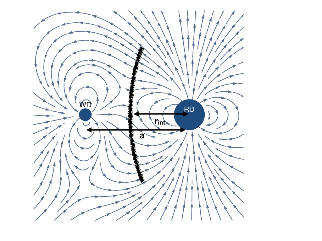
Figure 1: Cartoon of direct magnetospheric interaction. Pictured is a poloidal slice (in the plane containing the orbital momentum and the line connecting two stars) of the interacting magnetic field  of the WD and the RD. The hashed line indicates the location of the reconnection region, where field lines connect the surfaces of two stars. Orbital plane is horizontal, the magnetic moment of the WD is in the orbital plane, pointing at the moment towards the RD; the RD’s magnetic moment is along the orbits’ normal (pointing up); in the picture the magnetic moment of the RD is 5 times that of the WD. The structure of the magnetosphere is north-south asymmetric: in half a period of the WD’s rotation the asymmetry will reverse. Note: object sizes and distances are not to scale.

Assume that the stars have surface magnetic fields $B_{WD}$ and $B_{RD}$. For the given radii, $R_{WD}$ and $R_{RD}$ the force balance between two magnetospheres occurs at distance $r_{int}$ from the RD given by

$$\frac{r_{int}}{a}=\frac{1}{1+(R_{WD}/R_{RD})(B_{WD}/B_{RD})^{1/3}}=\frac{1}{1+\eta_{R}\eta_{B}^{1/3}}=\frac{1}{1+\eta_{\mu}}\mbox{}$$

$$\eta_{B}=B_{WD}/B_{RD}\gg 1\mbox{}$$

$$\eta_{R}=R_{WD}/R_{RD}=0.02\ll 1\mbox{}$$

$$\eta_{\mu}=\frac{\mu_{WD}}{\mu_{RD}}$$ (7)

M dwarfs can have surface magnetic fields $\sim 10^{3}$ G; as a result, the RD’s magnetosphere can extend beyond its Roche lobe. For a WD with surface magnetic field of $10^{6}$ G the balance between the magnetic fields will be at a distance $\sim 6.7\times 10^{10}$ cm - way inside the WD’s Roche lobe. Only for a very low magnetic field of the RD and extremely high magnetic field of the WD, so that $B_{WD}/B_{RD}\geq 10^{6}$, will the balance between magnetic pressures be inside the RD’s Roche lobe. Thus, the interaction between magnetospheres of the companions will generally be within the WD’s Roche lobe.

At the balance point, the local magnetic field is

$$\frac{B_{int}}{B_{WD}}=\frac{(1+\eta_{\mu}^{1/3})^{3}}{\eta_{B}}\left(\frac{R_{RD}}{a}\right)^{3}\approx\left(\frac{R_{RD}}{a}\right)^{3}\times\left\{\begin{array}[]{cc}\frac{1}{\eta_{B}},&\eta_{B}^{1/3}\eta_{R}\ll 1\\ \eta_{R}^{3}\left(\frac{R_{RD}}{a}\right)^{3},&\eta_{B}^{1/3}\eta_{R}\gg 1\end{array}\right.$$ (8)

In the particular case of AR Sco this requires $\eta_{B}\geq 10^{5}$; thus we expect $\eta_{B}^{1/3}\eta_{R}<1$. In this regime the magnetic field in the interaction region is independent of the magnetic field of the WD:

$$B_{int}\approx B_{RD}\left(\frac{R_{RD}}{a}\right)^{3}$$ (9)

Using (8) as an estimate of the magnetic field at the interaction region, $d_{int}\approx a-r_{int}$ (recall that $r_{int}$ is measured from the RD, and interaction size $R_{int}\approx a-r_{int}$, the spin-down power (5) becomes

$$L_{sd}=\frac{1}{4}\frac{(1+\eta_{\mu}^{1/3})^{3}}{\eta_{\mu}}\frac{B_{WD}^{2}R_{WD}^{6}\Omega_{WD}}{a^{3}}$$ (10)

where we expressed all the quantities in terms of WD’s parameters and the radial and magnetic ratios $\eta_{R}$ and $\eta_{B}$

In our case

$$\eta_{\mu}\equiv\left(\frac{R_{WD}}{R_{RD}}\right)^{3}\frac{B_{WD}}{B_{RD}}=8\times 10^{-6}\frac{B_{WD}}{B_{RD}}$$ (11)

For $B_{RD}\sim 10^{3}$ G it is likely to be much smaller than unity: $\eta_{\mu}\ll 1$. In this case (10) gives

$$L_{sd}=\frac{1}{4}\frac{B_{RD}B_{WD}R_{RD}^{3}R_{WD}^{3}\Omega_{WD}}{a^{3}}=\frac{1}{4}\frac{\mu_{WD}\mu_{RD}}{a^{3}}\Omega_{WD}$$ (12)

The required magnetic field is then

$$B_{WD}=4\frac{a^{3}\dot{\Omega}I_{WD}}{B_{RD}R_{RD}^{3}R_{WD}^{3}}=2\times 10^{7}{\rm G}$$ (13)

The necessary $\dot{M}$, Eq. (3), is still too high, $\dot{M}\sim 3\times 10^{-5}M_{\odot}$ yr^-1.

Thus we conclude that magnetospheric interaction, the most efficient of the scenarios considered, cannot accommodate the requirements of large current spin-down and efficient spin-up during the accretion stage. Importantly, the magnetically interacting magnetospheres cannot explain the WD’s spin-down, §2.3, yet this process is important for the generation of emission, as we will describe further in §4.

Below, in §3, we demonstrate that the WD’s spin-down can be easily explained due to mass loading of the RD’s wind onto the corotating WD’s magnetosphere.

3 The model of the WD’s torque: mass loading from the RD

In §2.1 we demonstrated that arguments in favor of high magnetic fields are untenable. We concluded then that the WD’s spin-down is due to the interaction with a companion. The key point then is to understand the WD-RD interaction and how it affects the WD spin-down and production of radiation. In this Section we discuss a model that can satisfy both the condition of large current spin-down, and the requirement of the low magnetic field from the spin-up conditions, as shown in Fig. 2.

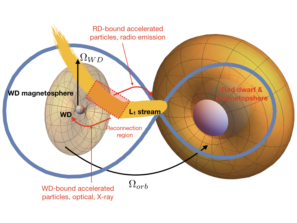
Figure 2: Cartoon of the model. The corotating magnetosphere of the WD extends beyond the WD’s Roche lobe and interacts with the wind/magnetosphere of the red dwarf. The red dwarf loses mass through the $L_{1}$ point. The partially ionized accretion stream loads the magnetosphere of the WD, providing large torque on the WD as it is ejected in the propeller regime. Previously, when the mass loss rate from the RD was high, the WD was spun-up in the accretor regime. Nonthermal particles are accelerated in the reconnection region between the RD’s accretion flow and the WD’s magnetosphere, producing optical and X-ray emission near the WD and radio emission near the RD.

3.1 Magnetic field of the WD must be low

We can estimate the WD’s magnetic field using the condition that for a given mass loss rate from the RD, $\dot{M}_{RD}$, accretion onto the WD spins up the latter. Using (3) with $r_{c}=r_{A}^{(a)}$ we find

$$B_{WD}=\frac{\sqrt{2}\dot{M}_{RD}^{1/2}(GM_{WD})^{5/6}}{R_{WD}^{3}\Omega_{WD}^{7/6}}=5\times 10^{5}{\rm G}$$ (14)

for the maximal accretion rate of $\dot{M}_{RD,max}\sim 10^{-9}M_{\odot}$ yr^-1 (Verbunt & Zwaan, 1981; Knigge et al., 2011). Thus, the WD’s magnetic field must be sufficiently low to allow spin-up.

3.2 Mass loading from spherical RD wind?

Let us first discuss a toy model with mass loading from a spherical RD wind. This simple approach will allow us to make estimates of the main parameters of the system. As we discuss below, §3.3.3, the actual mass loading occurs via Roche lobe overflow.

Assume that mass loading of the WD’s magnetosphere occurs at radius $r_{A}\approx v_{A}/\Omega$ with rate $\dot{M}_{WD}$. In the propeller regime (the current state) the loaded material is ejected with velocity $\sim r_{A}\Omega_{WD}$. The system is governed by the following set of conditions

$$L_{sd}=\dot{M}_{WD}(r_{A}\Omega_{WD})^{2}\mbox{}$$

$$v_{A}=\frac{B}{\sqrt{4\pi\rho}}\mbox{}$$

$$B=B_{WD}\left(\frac{r_{A}}{R_{WD}}\right)^{-3}$$ (15)

and

$$\dot{M}_{WD}=4\pi\rho v_{A}r_{A}^{2}\mbox{}$$

$$\dot{M}_{WD}=\frac{r_{A}^{2}}{4a^{2}}\dot{M}_{RD}$$ (16)

where we assumed that the relative fraction of the mass loaded onto WD’s magnetosphere is proportional to the mass loss rate of the RD $\dot{M}_{RD}$ and the relative fraction of the RD’s sky occupied by the interaction region, $\sim{r_{A}^{2}}/({4a^{2}})$.

Equation (16) gives

$$r_{A}=\frac{\sqrt{2a}L_{sd}^{1/4}}{\dot{M}_{RD}^{1/4}\Omega_{WD}^{1/2}}=2\times 10^{10}{\rm cm}\mbox{}$$

$$B_{WD}=\frac{(2a)^{3/4}L_{sd}^{7/4}}{\dot{M}_{RD}^{3/8}R_{WD}^{3}\Omega_{WD}^{5/4}}=3\times 10^{6}{\rm G}\mbox{}$$

$$\dot{M}_{WD}=\frac{\sqrt{\dot{M}_{RD}L_{sd}}}{2a\Omega_{WD}}=1.4\times 10^{-11}M_{\odot}{\rm yr}^{-1}$$ (17)

for $\dot{M}_{RD}=10^{-9}M_{\odot}{\rm yr}^{-1}$.

Thus, in order to account for the large spindown of the WD, the spherical accretion requires a very large mass loss rate from a RD. In the following, we develop model of WD’s mass loading through Roche lobe overflow and ensuing ionization.

3.3 Mass transfer via Roche lobe overflow

The atmospheres of RDs are relatively cold and dense; they are expected to be partially ionized. If the neutral-ion collision rate in the RD’s wind is not high (this is far from certain; see Garnavich et al., 2019), then the neutrals from the RD wind will stream freely onto the magnetic field lines of the WD. They will be exposed to the UV radiation from the surface of the WD that will lead to ionization. As the neutrals get ionized they will couple to the magnetic field of the WD, and will be centrifugally expelled from the system. Below we give order-of-magnitude estimates for the efficiency of ionization, leaving a more detailed analysis to a subsequent paper.

Next we discuss the RD-WD interaction that explains the key features of the WD’s spin-down due to loading of the WD’s magnetosphere by the partially ionized RD’ wind. We envision two possible scenarios: accretion onto the WD from a spherical wind from RD, §3.2, and accretion via a tightly confined matter stream caused by the Roche lobe overflow, §3.3.3.

3.3.1 The temperature of the WD

The ionization efficiency of the WD’s radiation depends sensitively on its surface temperature. Marsh et al. (2016) reported a surface temperature of $T_{WD}=9750$ K, although it may be as high as $T_{WD}\approx 12000$ K, as we describe below based on the analysis of Hubble Space Telescope (HST) data. This difference has important implications for the ionization processes in the wind, §3.3.2.

To constrain the WD’s effective temperature, we downloaded a grid of the Koester (2010) WD atmospheric models spanning a wide range of effective temperatures. We assumed a surface gravity of log(g) = 8.5. We then scaled the spectra to the Gaia distance of AR Sco (d=117 pc), assuming a WD radius of 7,000 km. Finally, we plotted the scaled spectra and compared them against the HST/Cosmic Origins Spectrograph(COS) spectrum (Marsh et al., 2016), Fig. 3.. We found that for $T_{WD}\gtrsim 13,000$ K, the WD’s photospheric contribution would be detectable in the HST spectrum, so we adopt this as a upper limit for the WD’s effective temperature.

A limitation of this approach is that the Koester (2010) models neglect magnetic effects. Given the unknown magnetic field strength of the WD, Zeeman splitting could have a significant impact on the WD’s photospheric lines. Higher signal-to-noise ratio UV spectra obtained around orbital phases when the system its faintest would provide more stringent limits on the WD properties.

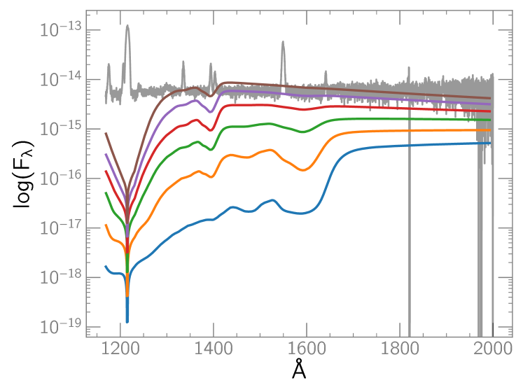
Figure 3: A comparison between the averaged HST/COS spectrum of AR Sco (grey line) and Koester (2010) WD models scaled to the Gaia distance. The observed spectrum is a sum of the WD contribution, the varying synchrotron radiation from the interaction, and line emission from the irradiated face of the secondary. The six colored lines represent WD models for log(g) = 8.5 and differ only in their effective temperatures. The temperatures range from 10,000 K (blue line) to 15,000 K (brown line) in increments of 1,000 K. Models with temperatures higher than 13,000 K predict that the photospheric contribution of the WD would be detectable, establishing an upper limit of $T_{WD}\leq 13000$ K for the WD temperature. As noted in the text, the Koester (2010) spectra neglect magnetic effects.

3.3.2 Ionization of the RD’s stream

For a WD surface temperature $T_{WD}\leq 12000$ K, §3.3.1, the number of photons emitted above the ionization threshold $\nu_{0}$ is

$$\dot{N}_{ph}=4\pi R_{WD}^{2}\int_{\nu_{0}}^{\infty}4\pi\frac{\nu^{2}}{c^{2}}\left(e^{h\nu/T}-1\right)^{-1}d\nu=5.5\times 10^{38}{\rm s}^{-1}$$ (18)

where $\nu_{0}=3.29\times 10^{15}$ Hz is the frequency corresponding to Hydrogen ionization. The corresponding mass loading rate for complete absorption would be $\dot{M}_{load}=m_{p}\dot{N}_{ph}=1.4\times 10^{-11}M_{\odot}{\rm yr}^{-1}$.

Also, the effective optical depth for ionization is of the order of unity

$$\sigma_{i}=\sigma_{0}(\nu/\nu_{0})^{-3}\mbox{}$$

$$n_{n}=\frac{\dot{M}_{RD}}{4\pi m_{p}a^{2}v_{w,RD}}$$ (19)

where $n_{n}$ is the density of neutrals, scaled to the RD mass loss rate of $10^{-9}M_{\odot}$ yr^-1, $\sigma_{i}$ is the ionization cross-section, in units of $\sigma_{0}=6.3\times 10^{-18}$ cm². Also, recombination time scales are mostly likely long enough. So the optical depth of the system for ionizing radiation is

$$\tau(\nu)\approx n_{n}\sigma_{i}a\approx 8000\frac{\dot{M}_{\rm RD,-9}}{a_{10.9}^{2}v_{w,7.5}}\left(\frac{\nu_{0}}{\nu}\right)^{3}.$$ (20)

The direct ionization radius can be estimated from equation

$$\frac{R_{\rm WD}^{2}}{r_{\rm io}^{2}}\int_{\nu_{0}}^{\infty}d\nu B_{\nu}\sigma_{i}=\frac{\max(v_{\rm w},v_{\rm ff})}{r_{\rm io}}$$ (21)

where $B_{\nu}$ is Planck’s spectrum

$$v_{\rm ff}=\sqrt{\frac{GM_{\rm WD}}{r_{\rm io}}}$$ (22)

even for $T_{\rm WD}=9750$ K and stellar wind with speed about 300 km/s the ionization radius evaluates to $r_{\rm io}\approx 5\times 10^{11}$ cm; this exceeds the orbital separation by more than 5 times.

In the previous estimation we neglect the absorption of ionizing photons by neutrals. Nevertheless, the secondary photons can ionize the matter in the stellar wind, the mass flux of neutrals can be balanced by ionizing photons flux or $\dot{N}_{ph}=\pi r_{io,max}^{2}v_{w}n_{n}$.

$$r_{\rm io,max}\approx\sqrt{\frac{\dot{N}_{ph}}{\pi n_{n}v_{\rm w,RD}}}\approx 1.9\times 10^{10}\dot{M}_{RD,-9}^{-1/2}a_{10.9}\mbox{ cm}$$ (23)

This corresponds to WD magnetosphere injection rate on the level

$$\dot{M}_{WD}\approx\frac{r_{\rm io,max}^{2}}{4a^{2}}\dot{M}_{\rm RD}\approx\dot{N}_{ph}m_{p}\approx 1.4\times 10^{-11}M_{\odot}/\mbox{yr}$$ (24)

So, if $r_{A}\geq r_{\rm io,max}$ in the spherically symmetric case the WD magnetosphere loading rate depends on ionizing photon production rate only.

Thus, we can estimate the mass loading rate using two different methods: Eq. (17) and Eq. (24). The required WD’s temperature is then $T_{WD}=12000$ K. In contrast, Marsh et al. (2016) estimated $T_{WD}\leq 9750$ K; this supplies $\sim 1/30$ of the required UV photon production rate. A new series of observations by HST at “off the peak” orbital phases could clarify this problem.

In conclusion, we expect that the WD’s radiation can ionize hydrogen in the outer parts of the RD’s corona, and in the surrounding area. On the other hand, if the mass flow from the RD is large, it can screen the ionizing radiation, so that the neutral component of the RD’s flow can penetrate the WD’s magnetosphere.

3.3.3 Mass transfer rates via Roche lobe overflow

Next we discuss a more realistic scenario based on mass transfer via Roche lobe overflow. In this case the main mass transfer process takes place through the first Lagrangian point $L_{1}$. As a result, the wind mass loss rate from the RD can be much smaller than for the spherical wind case discussed in the previous subsection §3.2. As a result, for smaller “effective” (isotropic-equivalent) mass loss rates, the radiation from the WD can ionize the photosphere of RD. Still the matter flowing through the $L_{1}$ point can contain neutral components.

In this case Eqns. (15) and (16) give

$$\dot{M}_{WD}\approx\eta_{s}\rho_{s}v_{A}r_{A}^{2}\mbox{}$$

$$\dot{M}_{WD}\approx\xi\dot{M}_{RD,stream}$$ (25)

here $\rho_{s}$ is density of the stream, $\eta_{s}$ is a constant order of 1 which take into account the geometry factor of the stream, $\xi$ is a fraction of the steam ionized and accelerated in WD magnetosphere.

$$r_{A}=\left(\frac{L_{sd}}{\xi\dot{M}_{RD,stream}\Omega_{WD}^{2}}\right)^{1/2}=2\times 10^{10}\,{\rm cm}\mbox{}$$

$$B_{WD}=\left(\frac{4\pi L_{sd}r_{A}^{3}}{\eta_{s}\Omega_{WD}R_{WD}^{6}}\right)^{1/2}=1.3\times 10^{7}\eta_{s}^{-1/2}{\rm G}$$ (26)

where $\xi\dot{M}_{RD,stream}\sim 10^{-11}M_{\odot}{\rm yr}^{-1}$ was assumed.

The $r_{A}$ and correspondingly $v_{A}$ are the same in Eq. (26) and Eq. (17), so the flow rate should be the same. Following the analysis in §3.2 we can estimate the magnetosphere mass loading rate due to ionization of neutrals flowing through the $L_{1}$ point and the ionizing photons number as

$$\dot{M}_{WD}\approx\frac{\dot{N}_{ph}m_{p}}{\eta_{s}}\approx 1.4\times 10^{-11}M_{\odot}/\mbox{yr}.$$ (27)

In the case of the flow from $L_{1}$ point, the ionization photons flux should be in $1/\eta_{s}$ if compared to the spherical wind case.

The source of the UV photons can be both the WD as well as the nonthermal synchrotron radiation from the interaction region. We hypothesize that in the latter case, a self-regulating quasi-periodic system evolves through the following ionization states: 1) “Plunging”: no nonthermal emission: the stream goes deeply into magnetosphere where it starts to be ionized; 2) “photoionization”: strong interactions between the ionized matter stream and magnetosphere produce nonthermal radiation which starts to ionize matter in the stream; and 3) ”quenching”: the strongly ionized stream stops penetrating and interacting with the WD magnetosphere, leading to suppression of nonthermal emission and returning the system to phase 1. So, the system will oscillate around the equilibrium state.

4 Emission model: acceleration at reconnection between interacting magnetospheres

4.1 Acceleration at reconnection

Interaction of the magnetic fields  between the WD’s and the RD’s magnetospheres will lead to reconnection. Particles will be heated and accelerated in the reconnection events. The reconnecting magnetic fields connect back to the WD and to the RD, where the accelerated particles will produce synchrotron/cyclotron emission within the corresponding magnetospheres. The synchrotron origin of optical emission at the WD is consistent with the highly linearly polarized optical signal, showing the polarization rotation (Buckley et al., 2017; du Plessis et al., 2019), similar to the rotating vector model in pulsars (Radhakrishnan & Cooke, 1969), see §4.2. The cyclotron origin of the radio emission in the RD is discussed in §4.3.

The reconnection events are expected to produce signal at the beat frequency between the WD’s spin and the orbital motion: as the field lines from different magnetic poles of the WD sweep by the MD, the polarity of the magnetic field in the wind changes every half a period. Depending on the orientation of the magnetic field of the MD, reconnection between the wind and MD’s magnetic field occurs every period.

The reconnection between the WD’s wind and MD’s magnetosphere should proceed in a somewhat typical fashion. The two plasma components have different plasma properties: very light WD’s magnetosphere and relatively heavy RD’s magnetosphere. Hence we expect different properties (density and temperature) on the two sides of any reconnection point.

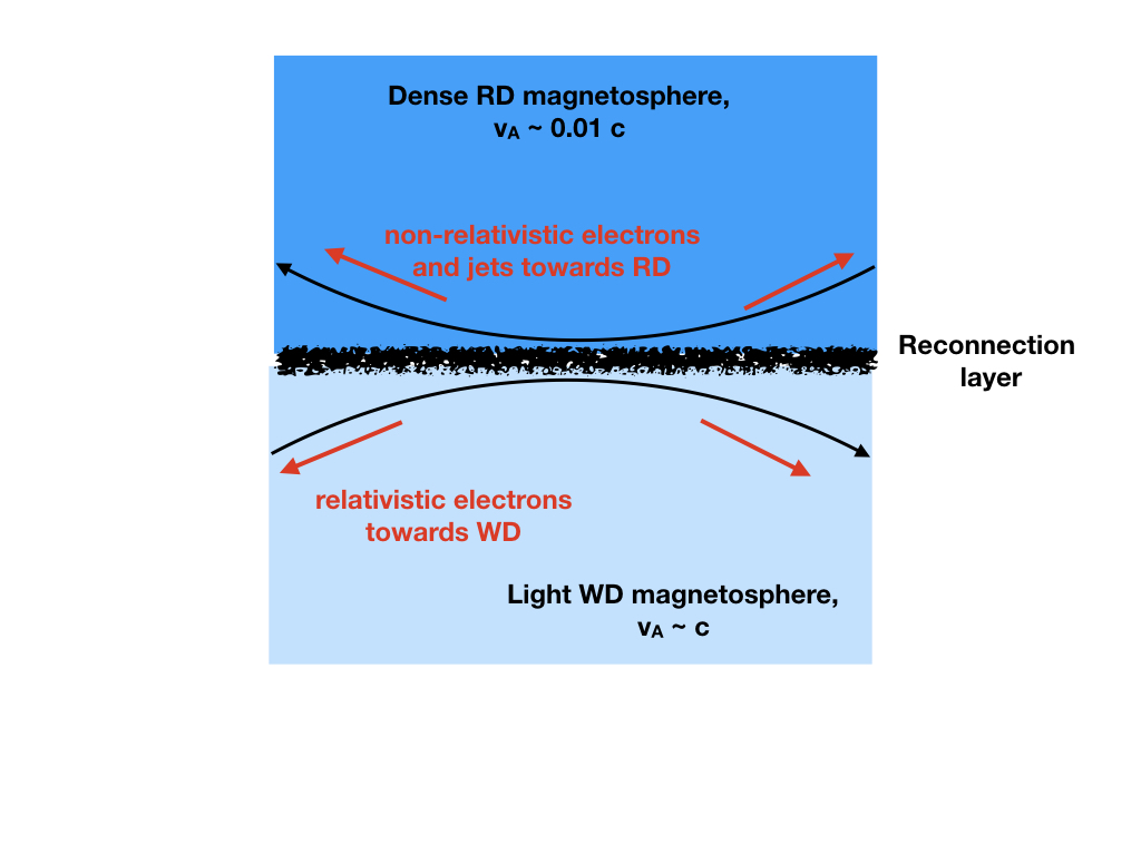
Figure 4: Asymmetric reconnection layer between the dense RD magnetosphere and the rarefied WD magnetosphere.

In the frame of our model we expect strong deformation of the WD’s magnetosphere due to interaction with stellar wind at the Alfvenic radius. Therefore, the plasma beta, $\beta=8\pi p/B_{int}^{2}\approx 1$. Reconnection in such plasmas proceeds in specific, unusual (from the classical point of view) regimes (e.g.,  Lyutikov et al., 2017a, b). Particles can be, under very extreme conditions, quickly accelerated up to the maximal available potential. The maximal Lorentz factor of particles can be then estimated as a potential across the reconnection region of size $\sim r_{A}$, magnetic field $B_{int}=B_{\rm WD}(r_{A}/R_{\rm WD})^{-3}\sim 200$ G and velocity of incoming magnetic field lines $\Omega r_{A}$ (so that electric field $E\sim({\Omega r_{A}}/{c})B_{int}$)

$$\gamma_{max}\approx\frac{e\Phi}{m_{e}c^{2}}\sim 10^{7}\mbox{}$$

$$\Phi\approx r_{A}\frac{\Omega r_{A}}{c}B_{int}$$ (28)

here we substitute values from Eq. 26. This is a very high Lorentz factor, but this is the upper estimate. As we demonstrate below, Eq. (32), the Lorentz factor  of the electrons accelerated towards the WD need to be $\sim 10^{-3}$ of the maximum possible value.

On the RD side the reconnection will be analogous to the solar magnetosphere, where particles are heated and produce UV and soft X-ray emission; this explains the X-ray emission from AR Sco. Non-relativistic exhaust jets that propagate with the local Alfvén velocity couple to the neutral component in the MD atmosphere/corona and generate H$\alpha$ features observed by Garnavich et al. (2019). Particles are also accelerated to mildly relativistic energies and produce radio emission both in the interaction region and within the RD corona.

4.2 Optical and X-ray emission: magnetosphere of the WD

We expect that in reconnection events particles are accelerated to power-law distributions. In the highly variable magnetic field of the WD’s magnetosphere particles accelerated in the interaction region will be propagating downward, increasing their emitted synchrotron frequency, while losing energy to synchrotron emission (and reflected due to magnetic bottling). It is a fairly complicated problem how to calculate synchrotron emission from a stream of particles propagating with the magnetospheres: (i) the basic cyclotron frequency $\omega_{B}$ changes with radius; (ii) in a collision-less plasma the particles’ pitch angles change with radius due to conservation of the first adiabatic invariant; (iii) the number of particles that reach a given radius changes due to the bottling effect; (iv) particle pitch angles evolves due to radiative losses (e.g.,  Lyutikov & Thompson, 2005). We leave a more detailed consideration to subsequent paper. Here we just provide order–of-magnitude estimates. In what follows we employ a concept that starting from the emission region with a pre-defined magnetic field, for a given emission frequency and radiated power there are optimal parameters to produce emission subject to the above constraints.

As an order-of-magnitude estimate, we assume that emission is dominated by particles with the synchrotron cooling time of the order of $c/r_{em}$ (lower energy particles do no emit efficiently since power $\propto\gamma^{2}$, while higher energy particles do not probe high magnetic fields). To produce synchrotron emission at a frequency $\omega$ and overall power $L_{s}\sim 10^{32}$ erg s^-1 we need the number of particles $N_{p}$ emitting typically at distance $r_{em}$ to be such that:

$$\omega\approx\gamma_{em}^{2}\omega_{B}\mbox{}$$

$$\tau_{c}\approx\frac{m_{e}c^{3}}{e^{2}\gamma_{em}\omega_{B}^{2}}=\frac{r_{em}}{c}\mbox{}$$

$$L_{s}\approx N_{p}\frac{e^{2}}{c}\gamma_{em}^{2}\omega_{B}^{2}$$ (29)

The above relations apply to particles in both magnetospheres,

$$B=B_{{WD}}\left(\frac{r_{em}}{R_{WD}}\right)^{-3}$$ (30)

where $B_{{WD}}$ and $R_{WD}$ stand for the surface magnetic field  and the radius of the corresponding star, and $r_{em}$ is the distance from the star’s surface. Resolving (29-30) we find

$$r_{em}=\frac{e}{m_{e}^{5/7}c^{11/7}}{B_{{WD}}^{3/7}R_{{WD}}^{9/7}\omega^{1/7}}\mbox{}$$

$$N_{p}=\frac{B_{{WD}}^{2/7}R_{{WD}}^{6/7}L_{s}}{c^{19/7}m_{e}^{8/7}\omega^{4/7}}\mbox{}$$

$$\gamma_{em}=\frac{e}{m_{e}^{4/7}c^{13/7}}{B_{{WD}}^{1/7}R_{{WD}}^{3/7}\omega^{5/7}}$$ (31)

Curiously, particles with very high energy radiate at higher frequencies further out.

For optical synchrotron emission with $L_{o}\sim 10^{32}$ erg s^-1

$$r_{em}=3.4\times 10^{9}\;\omega^{1/7}_{15}\mbox{ cm}\mbox{}$$

$$N_{p}=3\times 10^{34}\;L_{o,32}\omega^{-4/7}_{15}\mbox{}$$

$$\gamma_{em}=80\;\omega^{5/7}_{15}$$ (32)

Thus, relativistic particles in the WD magnetosphere emit optical emission at $\approx 10R_{WD}$. The amount of mass participating in the optical emission $\sim m_{p}N_{p}\approx 5\times 10^{10}$ g, is fairly small. The magnetic field in the optical emission region evaluates to $B_{em}\approx 2500\omega^{-3/7}_{15}$ G.

Takata et al. (2018) reported observations of AR Sco in the X-ray range with luminosity $L_{X}\sim 4\times 10^{30}$ erg s^-1. Corresponding relations for X-rays give

$$r_{em,X}=1.2\times 10^{10}\;\omega^{1/7}_{19}\mbox{ cm}\mbox{}$$

$$N_{p,X}=2\times 10^{32}\;\omega^{-4/7}_{19}\mbox{}$$

$$\gamma_{em,X}=6\times 10^{4}\;\omega^{5/7}_{19}$$ (33)

For $\omega_{X}\approx 10^{19}$ rad s^-1. The spectrum of the accelerated particles corresponds to $f\propto\gamma^{-p}$ with $p\approx 2$. All very reasonable numbers.

The inverse Compton scattering of electrons with Lorentz factors given in (32) on the WD’s photons with $\epsilon_{WD}\sim 1$ eV would produce similar frequencies, $\epsilon_{IC}\sim\gamma_{em}^{2}\epsilon_{WD}\sim 10^{4}\,{\rm eV}$. The electrons with the maximum Lorentz factor (28) would produce IC emission in the TeV range. Unfortunately, a magnetic energy density $U_{B}\approx B_{em}^{2}/8\pi\sim 10^{7}$ is much higher than the soft photon energy density $U_{ph}\sim L_{o}/4\pi cr_{em}^{2}\sim 30$, so for the leptonic model, the high energy emission can be estimated as $L_{HE}\sim L_{o}U_{ph}/U_{B}\sim 10^{26}$ erg/s. For a distance $\sim$100 pc we expect the observed flux to be $F_{HE}\sim 10^{-16}$ erg/s cm².

In conclusion, optical and X-ray emission from the system originates due to synchrotron emission of particles accelerated in reconnection events. Synchrotron cooling determines the typical location and luminosity.

4.3 Radio emission

The radio emissions from AR Sco paint a murky picture of the underlying physical processes that cause them. Marsh et al. (2016) found that AR Sco was a source of broadband, pulsed, $<$10% circularly polarized radio emission at high brightness temperatures ($T_{B}\sim 10^{12}-10^{14}$ K) for reasonable size estimates of the emitting region. Karl G. Jansky Very Large Array (VLA) observations of the system detected non-thermal emissions that were 0 to -27% circularly polarized on timescales of $\sim$10 min at 1.5 GHz, but only 0 to -8% at 5 and 9 GHz (Stanway et al., 2018). The measured linear polarization fractions were small, totaling 0-3%, and therefore much smaller than the degree of linear polarization measured at optical wavelengths. This small linear polarization fraction cannot be explained by synchrotron radio emission from the WD magnetosphere alone, again suggesting that AR Sco is not a “WD pulsar.”

We note that the observed properties of AR Sco bear many similarities to Jovian radio emission, as predicted by Willes & Wu (2004) in their work on the ECM-generated radio emissions anticipated to be found from planets that may orbit a WD. In our own solar system, Jupiter is a bright radio source of decametric emission (DAM), see review by Melrose (2017). DAM is nearly 100% circularly or elliptically polarized, and beamed in a hollow cone perpendicular to the source magnetic field, which indicates an ECM origin (Zarka, 1998). DAM emission is also driven by the binary interaction of magnetospheres - in this case of Jupiter’s magnetosphere with Io (Goldreich & Lynden-Bell, 1969). In this example, the emission is produced by the electrons accelerated by Io’s generated inductive electric field. Many of these observed properties qualitatively resemble the radio emission in AR Sco, which the present model also suggests is caused by the binary interaction of magnetospheres.

An alternative explanation for AR Sco’s radio emissions is gyrosynchrotron radiation. The standard flare scenario on the Sun and other main sequence stars is that reconnection in their magnetospheres accelerate electrons that emit mildly relativistic gyrosynchrotron radiation at radio wavelengths, and hard X-rays via bremsstrahlung when they interact with the denser layers of the corona (Bastian et al., 1998). This non-thermal emission mechanism extends to red dwarfs of spectral types as late as M9. These “ultracool dwarfs” are sources of quiescent, non-bursty, radio emissions at 2-8 GHz with circular polarization fractions $<$35% that have been the subject of extensive plasma physics modeling efforts (Metodieva et al., 2017; Zic et al., 2019). Within the AR Sco system, low circular polarization fractions, coupled with larger potential source region sizes imply the operation of an incoherent emission process such as gyrosynchrotron radiation.

In addition to polarization fraction and brightness temperature measurements, another means to distinguish between these two emission mechanisms is to leverage the Güdel-Benz relationship, which relates the thermalized X-ray luminosity generated by magnetic reconnection in stellar flares to the nonthermal, incoherent, gyrosynchrotron radio emission that results from particle acceleration (for a review, see Benz & Güdel (2010)). This relationship is given by

$${L_{X}\over L_{R}}\sim 10^{15.5\pm 0.5}~{}[Hz],$$ (34)

where $L_{X}$ is the X-ray luminosity and $L_{R}$ is the radio luminosity, usually computed as $\nu L_{\nu}$. Marsh et al. (2016) measured an X-ray luminosity of $L_{X}\approx 4.9\times 10^{30}$ erg s^-1 using Swift/X-ray Telescope (XRT), which corresponds to a Güdel-Benz relationship peak radio luminosity $\nu L_{\nu}\sim 4.9\times 10^{15}$ erg s^-1.

In contrast to this low expected radio luminosity, Marsh et al. (2016) measured a peak radio flux density of $F_{\nu,peak}\sim 15$ mJy at 9 GHz with the Australian Telescope Compact Array (ATCA), which corresponds to a peak radio luminosity of $\nu L_{\nu}\sim 2.3\times 10^{27}$ erg s^-1. This is far in excess of the radio emission generated by typical stellar flaring. The combination of moderate circular polarization fractions coupled with a greater-than-expected radio luminosity given the X-ray activity within the system indicates that both gyrosynchrotron and ECM processes must be present, caused by the complex interactions of the two magnetospheres.

Unlike X-ray and optical electrons which are accelerated to relativistic energies within the WD magnetosphere, the radio electrons are not cooling efficiently, hence estimates (29) are not applicable. The relatively large circular polarization fractions imply mildly relativistic electrons at most. The frequency of $9$ GHz can then be used to estimate the magnetic field on the RD: $B_{RD}\sim 3\times 10^{2}\gamma_{0.5}^{2}$ G, where we assume mildly relativistic electrons. The number of radio emitting electrons then estimates to

$$N_{r}\approx\frac{m_{e}^{2}c^{3}L_{r}}{e^{4}B_{RD}^{2}}\approx 7\times 10^{35}\gamma_{0.5}^{2}$$ (35)

We note that if ECM emission is present within the RD magnetosphere, there should exist a definite cutoff frequency, $\nu_{cf}$ beyond which radio emission is not detected that denotes the maximum magnetic field strength in the emitting region. The presence of this spectral feature would enable the direct calculation of the magnetic field strength and place constraints on the emitting plasma density (e.g.,  Route & Wolszczan, 2012).

Additional insight can be gained through analysis of the radio flux variation within the AR Sco system on timescales on the order of an orbital period. In Figure 4 of Stanway et al. (2018), the radio emissions from 1-10 GHz create a sinusoidal envelope with peak flux density $F_{\nu,peak}\sim 12$ mJy occurring near $\phi_{orb}\sim 0.5$, which corresponds to the WD being closest to the Earth. Although the radio flux density decreases to $F_{\nu}\sim 5$ mJy at $\phi_{orb}\sim 0$, it does not disappear entirely. This simple fact enables us to estimate that the RD contributes $\sim$40% of the system’s radio emission, while the remaining $\sim$60% is generated by the reconnection emission model described in §4. Similarly, the orbital modulation of the circular polarization fraction presents clues as to the location where cyclotron emission may arise. This fraction is maximal near $\phi_{orb}\sim-0.1$, when the observing geometry favors an unobstructed view of the RD hemisphere nearest the WD and the magnetospheric interaction region. Thus, these considerations support our model of magnetospheric interactions causing the nonthermal acceleration of electrons, which in the RD magnetosphere, result in additional cyclotron emission superimposed on intrinsic RD stellar flaring.

5 AE Aqr system and other polars

AE Aqr (Patterson, 1979; Wynn et al., 1997; de Jager et al., 1994) is the most rapidly rotating white dwarf known ($P_{\rm rot}=33.08$ s); it is also the most strongly asynchronous object ($P_{orb}=9.88$ hr) in the DQ Herculis class. AE Aqr is classified as a DQ Herculis-type cataclysmic variable, comprising a magnetized white dwarf primary and a K5 dwarf secondary. AE Aqr is characterized by coherent pulsations and quasi-periodic oscillations (QPOs) in the optical, UV, and soft X-ray wavelength bands. Although early work suggested that it is a source of 0.35-2.4 TeV $\gamma$-rays, later results from MAGIC and the FERMI Large Area Telescope (LAT) failed to confirm these purported detections (Meintjes et al., 1992; Aleksić et al., 2014; Li et al., 2016). In addition, AE Aqr displays violent flaring activity at optical, soft X-ray, and radio wavelengths.

We note in particular how the radio emission from AE Aqr differs from that found from AR Sco. Non-simultaneous, VLA observations of AE Aqr at 1.4, 4.9, 15, and 22.5 GHz revealed radio emission that varied on timescales of $\sim$5 min, with greater variability detected at higher frequencies (Bookbinder & Lamb, 1987; Bastian et al., 1988). No circular polarization was detected to within instrumental uncertainty ($\lesssim$15%) and the spectral index was found to vary from $\alpha\sim-1$ to 1.5. These results led Bookbinder & Lamb (1987) to suggest that synchrotron radiation from a mildly relativistic population of electrons ($\gamma\sim 3$) caused the radio emission, with the WD acting as an injector of electrons that are confined within the magnetic bottle of the secondary’s strong magnetic field. Alternatively, Bastian et al. (1988) argued that the radio emission represented the superposition of almost continually occurring synchrotron flares.

Let us apply the model to the AE Aqr. From (2) the required accretion rate during the spin-up stage is

$$\dot{M}=4\pi\frac{B_{WD}^{2}R_{WD}^{6}\Omega_{WD}^{7/3}}{(GM_{WD})^{5/3}}=\left\{\begin{array}[]{cc}10^{-7}B_{WD,6}^{2}&\mbox{for AR Sco}\\ 10^{-6}B_{WD,6}^{2}&\mbox{for AE Aqr}\end{array}\right.$$ (36)

Thus, smaller $\dot{M}$ is required for AE Aqr during the high stage; equivalently, its magnetic field can be somewhat higher. Our conclusion about the properties of AE Aqr are, generally, in agreement with those reached by Blinova et al. (2019).

Thus, the model places AR Sco (and AE Aqr) within a short-lived phase of IPs, with a very IP-like magnetic field strength. The AR Sco stage is short, $\sim 10^{6}-10^{7}$ yrs. Since, typically, the IP phase lasts $\sim 10^{9}$ years, several transitions to such a state can occur during the system’s lifetime.

What distinguishes AR Sco and AE Aqr from other intermediate polars? IPs typically have magnetic field $\sim 10^{7}$ G and are accreting. We suggest: (i) AR Sco and AE Aqr have smaller magnetic fields: the equilibrium spin is inversely proportional to the surface magnetic field  (for a given $\dot{M}$) - from (2) $\Omega\propto\dot{M}^{3/7}B_{WD}^{-6/7}$. Thus, small WD surface fields allow for faster equilibrium spin during the spin-up stage (low magnetic field  in AE Aqr was also proposed by Warner, 2004); (ii) currently AR Sco and AE Aqr are in a propeller regime due to their low accretion rates.

The present model also can be related to the “hibernating intermediate polar” model of Warner (2002), which proposes that the mass lost by the WD during a nova will cause the secondary to detach from its Roche lobe. The mass-transfer rate then drops to extremely low levels for very long periods of time. But before the system enters hibernation, there is a brief interval of enhanced mass transfer, caused by the irradiation of the secondary. Thus, various states of the system would involve: (i) high $\dot{M}$, accretion, spin-up; (ii) nova explosion, ejection of material; (iii) on Kelvin time scales the companion relaxes to a new detached state, and becomes a hibernating intermediate polar with very small $\dot{M}$.

6 Discussion

We develop a model of the highly asynchronous intermediate polars AR Sco and AE Aqr. The magnetic fields  of the WDs are relatively weak, $\sim 10^{7}$ G. They are currently in a transient propeller stage. The weak magnetic fields allowed a system to be in the accretor state during previous high mass transfer stage. As the WDs are spinning down quickly, each will eventually be in a double synchronous state like AM Herculis (Joss et al., 1979). The propeller stage in AR Sco does not even involve formation of the disk, but direct magnetospheric interaction with the companion. The fast spin-down of the WDs is determined by loading of the RD’s material and ensuing expulsion from the WDs’ magnetospheres in a transient propeller regime. If the mass accretion rate remains small, as it is now, each system will become synchronous and eventually will start accreting (this regime was studied numerically by Zhilkin et al., 2012; Isakova et al., 2019; Zhilkin et al., 2019). But if $\dot{M}$ increases, they will enter the earlier accretor regime.

In both systems, the mass loading of the WD’s magnetosphere by the partially ionized RD’s stream is strongly affected by the ionizing radiation from the WD. It leads to efficient loading of the WD’s magnetosphere needed to explain the high spin-down rate. The ionization conditions, we hypothesize, are what make the AR Sco and AE Aqr different: in our model the ionization of the RD’s flow by the WD is important, this difference in temperatures might affect the flow dynamics, as discussed at the end of Section 3.2.

We envision that most of the observed properties are determined by the direct interaction of the stars’ magnetospheres. This requires that the Alfvén points in the corresponding winds are further way from the stars than the $L_{1}$ point. This is easily achieved for the RD, since it is almost Roche lobe filling; in the case of WD it is required the the Alfvén velocity in the magnetosphere is larger that $v_{A}\geq(a\Omega_{WD})\approx 0.1c$. The magnetospheric/wind interaction of two stars is not responsible for the WD’s spin-down: it leads to the generation of the observed nonthermal emission by particles accelerated in reconnection events.

Finally, we point out that conventional models of spin and orbital evolution may have to be corrected in the case of AR Sco and AE Aqr. Interaction of the WD’s and RD’s magnetospheres also lead to a torque on the RD (Paczyński, 1967; Verbunt & Zwaan, 1981). Changing the spin of the RD, combined with the spin-orbital tidal synchronization, and the corresponding loss of the orbital angular momentum and the size of the RD’s Roche lobe, will lead to changes in the mass accretion rate. Using (12), we can estimate the mutual torque as

$$\dot{J}=-\frac{1}{4}\frac{\mu_{WD}\mu_{RD}}{a^{3}}=10^{33}{\rm erg}$$ (37)

for the parameters of AR Sco. This is the torque exerted on the RD due to magnetospheric interaction with the WD. This comes close to the general relativistic torque, which for the parameters of AR Sco, evaluates to $10^{34}$ erg. (In fact, Eq. (37) underestimates the torque, since it is applied at $r_{int}<a$.) We leave consideration of these effects to a subsequent paper.

References

- Abdo et al. (2013) Abdo, A. A., et al. 2013, ApJS, 208, 17
- Aleksić et al. (2014) Aleksić, J., et al. 2014, A&A, 568, A109
- Barlow et al. (2006) Barlow, E. J., Knigge, C., Bird, A. J., J Dean, A., Clark, D. J., Hill, A. B., Molina, M., & Sguera, V. 2006, MNRAS, 372, 224
- Barrett et al. (2017) Barrett, P. E., Dieck, C., Beasley, A. J., Singh, K. P., & Mason, P. A. 2017, AJ, 154, 252
- Bastian et al. (1998) Bastian, T. S., Benz, A. O., & Gary, D. E. 1998, ARA&A, 36, 131
- Bastian et al. (1988) Bastian, T. S., Dulk, G. A., & Chanmugam, G. 1988, ApJ, 324, 431
- Benz & Güdel (2010) Benz, A. O., & Güdel, M. 2010, ARA&A, 48, 241
- Beuermann (1999) Beuermann, K. 1999, in Highlights in X-ray Astronomy, ed. B. Aschenbach & M. J. Freyberg, Vol. 272, 410
- Blinova et al. (2019) Blinova, A. A., Romanova, M. M., Ustyugova, G. V., Koldoba, A. V., & Lovelace, R. V. E. 2019, MNRAS, 487, 1754
- Bookbinder & Lamb (1987) Bookbinder, J. A., & Lamb, D. Q. 1987, ApJ, 323, L131
- Buckley et al. (2017) Buckley, D. A. H., Meintjes, P. J., Potter, S. B., Marsh, T. R., & Gänsicke, B. T. 2017, Nature Astronomy, 1, 0029
- de Jager et al. (1994) de Jager, O. C., Meintjes, P. J., O’Donoghue, D., & Robinson, E. L. 1994, MNRAS, 267, 577
- du Plessis et al. (2019) du Plessis, L., Wadiasingh, Z., Venter, C., & Harding, A. K. 2019, arXiv e-prints, arXiv:1910.07401
- Eggleton (1983) Eggleton, P. P. 1983, ApJ, 268, 368
- Fawley et al. (1977) Fawley, W. M., Arons, J., & Scharlemann, E. T. 1977, ApJ, 217, 227
- Ferrario et al. (2015) Ferrario, L., de Martino, D., & Gänsicke, B. T. 2015, Space Sci. Rev., 191, 111
- Garnavich et al. (2019) Garnavich, P., Littlefield, C., Kafka, S., Kennedy, M., Callanan, P., Balsara, D. S., & Lyutikov, M. 2019, ApJ, 872, 67
- Goldreich & Julian (1969) Goldreich, P., & Julian, W. H. 1969, ApJ, 157, 869
- Goldreich & Lynden-Bell (1969) Goldreich, P., & Lynden-Bell, D. 1969, ApJ, 156, 59
- Ikhsanov (1998) Ikhsanov, N. R. 1998, A&A, 338, 521
- Ikhsanov & Beskrovnaya (2008) Ikhsanov, N. R., & Beskrovnaya, N. G. 2008, arXiv e-prints, arXiv:0809.1169
- Ikhsanov & Beskrovnaya (2012) —. 2012, Astronomy Reports, 56, 595
- Ikhsanov & Biermann (2006) Ikhsanov, N. R., & Biermann, P. L. 2006, A&A, 445, 305
- Isakova et al. (2019) Isakova, P. B., Zhilkin, A. G., & Bisikalo, D. V. 2019, INASAN Science Reports, 3, 194
- Joss et al. (1979) Joss, P. C., Katz, J. I., & Rappaport, S. 1979, ApJ, 230, 176
- Kaplan et al. (2019) Kaplan, Q., Meintjes, P. J., Singh, K. K., van Heerden, H. J., Ramamonjisoa, F. A., & van der Westhuizen, I. P. 2019, arXiv e-prints, arXiv:1908.00283
- Katz (2017) Katz, J. I. 2017, ApJ, 835, 150
- Knigge et al. (2011) Knigge, C., Baraffe, I., & Patterson, J. 2011, ApJS, 194, 28
- Koester (2010) Koester, D. 2010, Mem. Soc. Astron. Italiana, 81, 921
- Li et al. (2016) Li, J., Torres, D. F., Rea, N., de Oña Wilhelmi, E., Papitto, A., Hou, X., & Mauche, C. W. 2016, ApJ, 832, 35
- Lyutikov et al. (2017a) Lyutikov, M., Sironi, L., Komissarov, S. S., & Porth, O. 2017a, Journal of Plasma Physics, 83, 635830601
- Lyutikov et al. (2017b) —. 2017b, Journal of Plasma Physics, 83, 635830602
- Lyutikov & Thompson (2005) Lyutikov, M., & Thompson, C. 2005, ApJ, 634, 1223
- Marsh et al. (2016) Marsh, T. R., et al. 2016, Nature, 537, 374
- Meintjes et al. (1992) Meintjes, P. J., Raubenheimer, B. C., de Jager, O. C., Brink, C., Nel, H. I., North, A. R., van Urk, G., & Visser, B. 1992, ApJ, 401, 325
- Melrose (2017) Melrose, D. B. 2017, Reviews of Modern Plasma Physics, 1, 5
- Metodieva et al. (2017) Metodieva, Y. T., Kuznetsov, A. A., Antonova, A. E., Doyle, J. G., Ramsay, G., & Wu, K. 2017, MNRAS, 465, 1995
- Paczyński (1967) Paczyński, B. 1967, Acta Astron., 17, 287
- Patterson (1979) Patterson, J. 1979, ApJ, 234, 978
- Radhakrishnan & Cooke (1969) Radhakrishnan, V., & Cooke, D. J. 1969, Astrophys. Lett., 3, 225
- Rees & Gunn (1974) Rees, M. J., & Gunn, J. E. 1974, MNRAS, 167, 1
- Route & Wolszczan (2012) Route, M., & Wolszczan, A. 2012, ApJ, 747, L22
- Stanway et al. (2018) Stanway, E. R., Marsh, T. R., Chote, P., Gänsicke, B. T., Steeghs, D., & Wheatley, P. J. 2018, A&A, 611, A66
- Sturrock (1971) Sturrock, P. A. 1971, ApJ, 164, 529
- Takata et al. (2018) Takata, J., Hu, C. P., Lin, L. C. C., Tam, P. H. T., Pal, P. S., Hui, C. Y., Kong, A. K. H., & Cheng, K. S. 2018, ApJ, 853, 106
- Toloza et al. (2019) Toloza, O., et al. 2019, BAAS, 51, 168
- Usov (1988) Usov, V. V. 1988, Soviet Astronomy Letters, 14, 258
- Verbunt & Zwaan (1981) Verbunt, F., & Zwaan, C. 1981, A&A, 100, L7
- Warner (1995) Warner, B. 1995, Astronomical Society of the Pacific Conference Series, Vol. 85, The Discovery Of Magnetic Cataclysmic Variable Stars, ed. D. A. H. Buckley & B. Warner, 3
- Warner (2002) Warner, B. 2002, in American Institute of Physics Conference Series, Vol. 637, Classical Nova Explosions, ed. M. Hernanz & J. José, 3–15
- Warner (2003) —. 2003, Cataclysmic Variable Stars
- Warner (2004) —. 2004, PASP, 116, 115
- Wickramasinghe & Ferrario (2000) Wickramasinghe, D. T., & Ferrario, L. 2000, PASP, 112, 873
- Willes & Wu (2004) Willes, A. J., & Wu, K. 2004, MNRAS, 348, 285
- Wynn et al. (1997) Wynn, G. A., King, A. R., & Horne, K. 1997, MNRAS, 286, 436
- Zarka (1998) Zarka, P. 1998, J. Geophys. Res., 103, 20159
- Zhilkin et al. (2012) Zhilkin, A. G., Bisikalo, D. V., & Boyarchuk, A. r. A. 2012, Physics Uspekhi, 55, 115
- Zhilkin et al. (2019) Zhilkin, A. G., Sobolev, A. V., Bisikalo, D. V., & Gabdeev, M. M. 2019, Astronomy Reports, 63, 751
- Zic et al. (2019) Zic, A., Lynch, C., Murphy, T., Kaplan, D. L., & Chandra, P. 2019, MNRAS, 483, 614