Guiding Robot Exploration in Reinforcement Learning via Automated Planning

Abstract

Reinforcement learning (RL) enables an agent to learn from trial-and-error experiences toward achieving long-term goals; automated planning aims to compute plans for accomplishing tasks using action knowledge. Despite their shared goal of completing complex tasks, the development of RL and automated planning has been largely isolated due to their different computational modalities. Focusing on improving RL agents’ learning efficiency, we develop Guided Dyna-Q (GDQ) to enable RL agents to reason with action knowledge to avoid exploring less-relevant states. The action knowledge is used for generating artificial experiences from an optimistic simulation. GDQ has been evaluated in simulation and using a mobile robot conducting navigation tasks in a multi-room office environment. Compared with competitive baselines, GDQ significantly reduces the effort in exploration while improving the quality of learned policies.

1 Introduction

Recent advances in artificial intelligence have enabled robots to conduct a variety of service and interaction tasks in human-inhabited environments (Hawes et al. 2017; Khandelwal et al. 2017; Veloso 2018). When a world model of dynamics and rewards is available, one can use Markov decision process (MDP) algorithms to compute action policies (Puterman 2014). In practice, however, world models are frequently unavailable or tend to change over time due to exogenous changes. Reinforcement learning (RL) algorithms have been used to help agents learn action policies from trial-and-error experiences toward maximizing long-term utilities (Sutton and Barto 2018).

There are various types of RL algorithms. Model-based RL enables agents to learn a world model while learning an action policy to achieve long-term goals (Brafman and Tennenholtz 2002; Mann and Choe 2011; Kaiser et al. 2020). Model-based RL can easily incorporate domain knowledge, such as world dynamics, from a human expert into the process of policy learning. In addition, model-based RL is goal-independent from the model construction perspective, rendering the learned world model applicable to other tasks. The learned model cannot represent all dynamics, and thus, model-based RL can be susceptible to domain changes. We are still interested in model-based RL in this work acknowledging its limitations, due to the characteristics of service robotics domains, such as widely available domain knowledge (e.g., how rooms are connected through doors), and highly diverse service requests (e.g., requests of guiding visitors from and to different indoor locations).

In this paper, we focus on addressing the low sample-efficiency challenge of model-based RL algorithms. We develop Guided Dyna-Q (GDQ) that consolidates the two classical paradigms of model-based RL and automated planning to help the agent avoid exploring less-relevant states toward more sample-efficient model learning and decision making. GDQ reasons with action knowledge to optimistically simulate action sequences to “accomplish” tasks. The simulated experience is then used to initialize and update Q-values toward efficient policy learning. In particular, we use Answer Set Programming (ASP) to formulate action knowledge (Lifschitz 2019), and use Dyna-Q for model-based RL (Sutton and Barto 2018), though GDQ is not restricted to particular planning or learning paradigms. It should be noted that we only use widely available action knowledge, such as “To open a door, one has to be in front of it first,” where knowledge acquisition is not a problem. The goal is to improve the learning efficiency in service robotics domains, and show that GDQ can leverage the complementary features of learning and planning paradigms to produce the best performance. We summarize GDQ, including the interplay between RL and automated planning, in Figure 1.

We have evaluated GDQ in simulation, and demonstrated the learning process using a real mobile robot. Results show that GDQ significantly improves the learning efficiency in comparison to existing model-based and model-free RL methods, including Q-Learning and Dyna-Q (Sutton and Barto 2018), as well as a competitive baseline that uses action knowledge to guide RL (Leonetti, Iocchi, and Stone 2016). In a real-world office environment with more than 20 rooms, GDQ helped a mobile robot learn the optimal solution from only 30 episodes, whereas vanilla Dyna-Q could not find a meaningful solution in a reasonable runtime.

Figure 1: An overview of Guided Dyna-Q (GDQ), where the key is the interplay between an automated planner and a reinforcement learner. The red-color loop corresponds to the standard control loop of Dyna-Q, where the agent (robot) interacts with the environment to update both its world model, and its $Q$-value function. Beyond that, GDQ further incorporates an automated planner into the learning process in the blue-color loop where goal-independent action knowledge (highly sparse, and potentially inaccurate) is used for computing action sequences toward goal achievement. The action sequences are then used for updating both the world model and the $Q$-value function.

2 Background

In this section, we briefly summarize the concepts of reinforcement learning and automated planning.

2.1 Reinforcement Learning

Within the MDP context, the agent must learn action policies from trial-and-error experiences when world models (reward functions, transition functions, or both) are not known. For instance, Q-learning is a model-free RL algorithm, and its $Q$-value function can be updated as below.

$$Q(s,a)\leftarrow Q(s,a)+\alpha\left[r+\gamma\max_{a^{\prime}}Q(s^{\prime},a^{\prime})-Q(s,a)\right]$$

where $r$ is the immediate reward after taking action $a$ in state $s$. This update procedure enables the agent to incrementally learn from every single $(s,a,s^{\prime},r)$ sample.

Model-based RL algorithms learn the world model, including $\mathcal{R}(s,a)$ and $\mathcal{T}(s,a,s^{\prime})$, and then use planning algorithms to compute the action policy. Dyna-Q (Sutton 1991) is a model-based RL framework, and includes the two primary components of model-free RL (Q-learning) and probabilistic planning (e.g., value iteration). The real-world interaction experience is used for two purposes in Dyna-Q: world model learning, and action policy learning. Besides, Dyna-Q is able to generate extra (simulation) experience through interacting with the learned world model, which further speeds up the policy learning process. We use declarative action knowledge to prevent the Dyna-Q agent from exploring less-relevant states.

We use Dyna-Q as a building block in the implementation of GDQ, because it is simple and has been widely studied in the RL literature. It should be noted that GDQ practitioners can replace Dyna-Q with other model-based RL methods.

2.2 Automated Planning

Automated planning methods aim at computing a sequence of actions toward accomplishing complex tasks (Ghallab, Nau, and Traverso 2016). One has to declaratively encode action knowledge into an automated planner, including actions’ preconditions and effects. Since the development of STRIPS (Fikes and Nilsson 1971), many action languages have been developed for formally representing action knowledge. The following shows an example of using STRIPS to formulate action ştack, where preconditions include the robot arm holding object X̧ and object Y̧ being clear. Executing this action causes the hand to be empty, and object Y̧ not clear anymore.

operator(stack(X,Y),
         Precond [holding(X),clear(Y)],
         Add [handempty,on(X,Y),clear(X)],
         Delete [holding(X),clear(Y)])

There are a number of action languages that can be used for encoding action knowledge, including PDDL that has been widely used in real-world planning systems (McDermott et al. 1998). Answer set programming (ASP) is a general-purpose knowledge representation and reasoning paradigm, and supports automated planning (Lifschitz 2019). We use ASP in this research mainly because of its good performance in knowledge-intensive domains (Jiang et al. 2019b). For instance, in navigation tasks, the robot needs to reason about potentially many rooms and their connections. The action knowledge we use is simple and publicly available (Yang et al. 2014; Jiang et al. 2019b), so we do not discuss knowledge acquisition in this paper.

3 Algorithm

In this section, we present Guided Dyna-Q (GDQ), the key contribution of this research. GDQ leverages goal-independent action knowledge for sample-efficient policy learning by enabling the interplay between a model-based reinforcement learner and an automated planner.

We use $\Pi(\mathcal{S}^{A},\mathcal{A}^{A},M)$ to represent our automated planner, where $\mathcal{S}^{A}$ and $\mathcal{A}^{A}$ are the state and action sets respectively. A task to the automated planner is defined as $M=(s^{A}_{0},s^{A}_{G})$ where $s^{A}_{0},s^{A}_{G}\in\mathcal{S}^{A}$ are the initial state and goal states respectively. For simplification, the goal is defined as a single state, though it can be a set of states in practice. Given task $M$, an automated planning system can use $\Pi(\mathcal{S}^{A},\mathcal{A}^{A},M)$ to compute a set of plans, $\mathcal{H}$, where $p\in\mathcal{H}$ is in the form of a sequence of state-action pairs, and each action sequence leads state transitions from the initial state $s^{A}_{0}$ all the way to the goal state $s^{A}_{G}$.

$$p=\left<\left<s^{A}_{0},a^{A}_{0}\right>,\left<s^{A}_{1},a^{A}_{1}\right>,\cdots,\left<s^{A}_{G}\right>\right>$$

We use an automated planning system (Gebser et al. 2011) that supports “optimisation statements” for generating a set of the shortest plans (action costs are not considered in this process). In order to enable the reinforcement learner to exploit the plans, we introduce a mapping function, $\mathcal{O}$, that constructs the correspondence between the planner’s action space $\mathcal{A}^{A}$ and the learner’s action space $\mathcal{A}$, and the correspondence between their state spaces $\mathcal{S}^{A}$ and $\mathcal{S}$.

$$\forall s^{A}\!\!\in\!\mathcal{S}^{A},~{}\forall a^{A}\!\!\in\!\mathcal{A}^{A}(s^{A}),~{}s\!\in\!\mathcal{O}^{-1}(s^{A})\Rightarrow s\!\in\!\mathcal{S},~{}a\!\in\!\mathcal{A}(s)$$

where $\mathcal{A}(s)\subseteq\mathcal{A}$, and $a\in\mathcal{A}(s)$ is applicable in state $s$.

Next, we describe how the plans generated by the automated planner are used for optimistic initialization (Section 3.1), policy update (Section 3.2), and their integration, i.e., the GDQ algorithm.

Algorithm 1 Optimistic Initialization: OptInit

Input: $\mathcal{S}$, $\mathcal{A}$, $\mathcal{S}^{A}$, $\mathcal{A}^{A}$, $M=(s^{A}_{0},s^{A}_{G})$
Parameter: $\gamma$, $\alpha$, $R_{max}$
Output: $\pi$

1:  for $\forall s\in\mathcal{S},a\in\mathcal{A}(s)$ do {Initialize Q-values, $\mathcal{R}$, and $\mathcal{T}$}

2:     $Q(s,a)\leftarrow 0.0$; $\mathcal{R}(s,a)\leftarrow 0.0$; $\mathcal{T}(s,a,s_{0})\leftarrow 1.0$

3:  end for

4:  $\mathcal{H}\leftarrow\Pi(\mathcal{S}^{A},\mathcal{A}^{A},M)$ {Compute a set of optimistic plans}

5:  for $p$ in $\mathcal{H}$ do

6:     for $\left<s^{A},a^{A}\right>$ in $p$ do

7:        $s,a\leftarrow\mathcal{O}(s^{A})$

8:        $\mathcal{R}(s,a)\leftarrow R_{max}$ {Optimistically update $\mathcal{R}$}

9:     end for

10:  end for

11:  $\pi\leftarrow\text{random policy}$ {Randomly initialize a policy}

12:  while $\pi\neq\pi^{\prime}$ do

13:     $\pi^{\prime}\leftarrow\pi$

14:     for $\forall s\in\mathcal{S}$ do

15:        $Q(s,\!\pi(s))\!\!\leftarrow\!\!\mathcal{R}(s,\!\pi(s))\!+\!\gamma\!\!\!\sum\limits_{s^{\prime}\in\mathcal{S}}\!\!\mathcal{T}(s,\!\pi(s),\!s^{\prime})Q(s^{\prime}\!,\!\pi(s^{\prime}))$

16:        $\pi(s)\leftarrow\text{argmax}_{a}Q(s,a)$

17:     end for

18:  end while

19:  return $\pi$

3.1 Optimistic Initialization

The plans computed by the automated planner are referred to as optimistic plans, because real-world domain uncertainty is frequently overlooked in building the planners. For instance, a robot taking the action of “navigate to room R” sometimes does not result in the robot being in room R due to the possibility of obstacles blocking the way. The goal of optimistic initialization (OptInit) is to use the plans computed by the automated planner to initialize Q-values, and prevent the agent from exploring less-relevant states.

Algorithm 1 presents our optimistic initialization process. The input includes the state and action spaces of both the reinforcement learner and the automated planner. $M$ is the provided task. The output is an initial policy $\pi$, which is generated by the agent interacting with the world.

Lines 1-3 are used for initializing the Q-values, as well as the transition and reward functions. The transition function is initialized in a way that all state-action pairs deterministically lead to the initial state. This setting is necessary because all plans computed by the automated planner start from the initial state. Given task $M=(s^{A}_{0},s^{A}_{G})$, our automated planner computes a set of optimistic plans in Line 4. The two for-loops in Lines 5-10 assign the highest reward, $R_{max}$, to the reward of all state-action pairs that appear in the plans from our automated planner. This is similar to how R-MAX realizes the trade-off between exploration and exploitation (Brafman and Tennenholtz 2002). Lines 12-18 are used for computing an action policy using policy iteration. Finally, the computed policy is returned in Line 19.

It should be noted that the agent has not started interacting with the environment while running OptInit (Algorithm 1). This initialization process enables the agent to prioritize states that are more relevant to the current task when exploring its working environment, which enables the agent to accomplish tasks more efficiently.

Algorithm 2 Policy Update: PolicyUp

Input: $\mathcal{S}$, $\mathcal{A}$, $\mathcal{S}^{A}$, $\mathcal{A}^{A}$, $M=(s^{A}_{0},s^{A}_{G})$, $\pi$, $C$, $R_{sum}$
Parameter: $\gamma$, $\alpha$, $R_{max}$, $m$, $N$
Output: $\mathcal{R},\mathcal{T},\pi$

1:  Collect the current world state $s$ from the world

2:  $a\leftarrow$ $\pi(s)$, with $\epsilon$ exploration rate

3:  Collect resulting state $s^{\prime}$ and reward $r$ after taking $a$

4:  Update the Q-value using real interaction experience$Q(s,a)\leftarrow Q(s,a)+\alpha[r+\gamma\max_{a^{\prime}}Q(s^{\prime},a^{\prime})-Q(s,a)]$

5:  $C(s,a,s^{\prime})\leftarrow C(s,a,s^{\prime})+1$

6:  $R_{sum}(s,a)\leftarrow R_{sum}(s,a)+r$

7:  if $\sum_{s^{\prime}}{C(s,a,s^{\prime})}>m$ then

8:     $\mathcal{T}(s,a,s^{\prime})\leftarrow C(s,a,s^{\prime})/\sum_{s^{\prime\prime}}{C(s,a,s^{\prime\prime})}$

9:     $\mathcal{R}(s,a)\leftarrow R_{sum}(s,a)/\sum_{s^{\prime\prime}}{C(s,a,s^{\prime\prime})}$

10:  end if

11:  $M\leftarrow(\mathcal{O}(s),s^{A}_{G})$

12:  $\mathcal{H}\leftarrow\Pi(\mathcal{S}^{A},\mathcal{A}^{A},M)$ {Compute a set of plans}

13:  for $n$ in $\{1\cdots N\}$ do

14:     $p\leftarrow\text{randomly selected plan in }\mathcal{H}$

15:     $\left<s^{A},a^{A}\right>\leftarrow\text{randomly selected transition in }p$

16:     $s,a\leftarrow\mathcal{O}^{-1}(s^{A})$

17:     Update $Q(s,a)$ using Bellman equation.

18:  end for

19:  $\forall s\in\mathcal{S},\forall a\in\mathcal{A},\pi(s)\leftarrow\text{argmax}_{a}Q(s,a)$

20:  return $\mathcal{R},\mathcal{T},\pi$

3.2 Policy Update and GDQ

The previous subsection (Section 3.1) presents the process of initializing the Q-function using the optimistic plans generated by our automated planner. Given the initialized $Q$-value function, the agent is able to compute an initial policy, and use this policy to interact with the real world. This subsection describes how the interaction experience, along with the automated planner, is used to update the $Q$-value function at runtime. Intuitively, the automated planner serves as an optimistic simulator to enable the reinforcement learner to learn from interaction experience in simulation.

Algorithm 2 presents the policy update process. Its input includes an action policy, a counter function $C$, and a reward counter function $R_{sum}$, in addition to the input of Algorithm 1. This policy is provided by Algorithm 1. Parameter $m$ is a threshold, representing how many times a state-action pair has been selected. Parameter $N$ is used for determining how many state-action pairs are simulated using the automated planner. The output includes not only a policy, but also the reward and transition functions, because our reinforcement learner is model-based.

Lines 1-4 are used for interacting with the real world using the current action policy, $\pi$. Then, $C(s,a,s^{\prime})$ is increased by one for updating the number of state-action-state triples. If the agent has visited a state-action pair for more than $m$ times (Line 7), the transition and reward functions are updated. Intuitively, $m$ is a parameter that indicates a state-action pair being known or unknown. In Line 12, the automated planner generates a set of plans. Using the generated plans, we randomly select one transition from a randomly-selected plan $p\in\mathcal{H}$, and update the Q-value accordingly. This Q-value update process is repeated for $N$ times in Lines 13-18. Finally, the reward function, transition function, and updated policy are returned.

Algorithm 3 is simply an integration of the two sub-procedures for optimistic initialization (Algorithm 1) and repeatedly conducted runtime policy update (Algorithm 2), which identifies the main contribution of this research. Informally, Algorithm 1 helps the agent avoid the near-random exploration behaviors through a “warm start” enabled by our automated planner, and Algorithm 2 guides the agent to only try the actions (in the real world) that can potentially lead to the ultimate goal. Next, we present an instantiation of GDQ followed by our experiment setup, and experimental results from comparisons between GDQ and a number of baseline methods selected from the literature.

Algorithm 3 Guided Dyna-Q (GDQ)

Input: $\mathcal{S}$, $\mathcal{A}$, $\mathcal{S}^{A}$, $\mathcal{A}^{A}$, $M=(s^{A}_{0},s^{A}_{G})$, $\pi$, $C$
Output: $\pi$

1:  Call Algorithm-1: $\pi\leftarrow\textsc{OptInit}(\mathcal{S},\mathcal{A},\mathcal{S}^{A},\mathcal{A}^{A},M)$

2:  $\forall s\in\mathcal{S},\forall a\in\mathcal{A},\forall s^{\prime}\in\mathcal{S},C(s,a,s^{\prime})\leftarrow 0,R_{sum}(s,a)\leftarrow 0$

3:  while Current state $s$ is not terminal do

4:     Call Algorithm-2:

$$\mathcal{R},\mathcal{T},\pi\leftarrow\textsc{PolicyUp}(\mathcal{S},\mathcal{A},\mathcal{S}^{A},\mathcal{A}^{A},M,\pi,C,R_{sum})$$

5:  end while

6:  return $\pi$

3.3 GDQ Instantiation

While GDQ is a general-purpose algorithm for knowledge-based RL, its implementation requires a task planner that is domain-dependent (still task-independent). We consider a mobile robot navigation domain, where the robot needs to navigate in an indoor office environment. The rooms, including hallways, are connected through doors that are of different sizes. Big doors are more friendly to the robot, though the robot needs to learn the “success rate” of navigating through doors from trial and error. Our robot does not have an arm and hence needs human help to open doors. Some doors are located in areas where human help is better available, while in some areas the robot might have to wait a long time until people show up to help.

In each trial (episode), the robot is tasked with navigating from its initial position to a goal position. There are doors connecting rooms and corridors, and there are different costs and success rates in navigation and door opening actions. The robot has four types of actions of goto(P,I), approach(D,I), opendoor(D,I), and gothrough(D,I) for navigational purposes, where P is one of the 19 positions, D is one of the 6 doors, and I is the step number. The actions and parameters together form a large action space for our RL agent. As an example, the following rule defines the effect of action gothrough(D,I),

at(R2,I+1):- gothrough(D,I),
            at(R1,I), acc(R1,D,R2), I<n.

where acc(R1,D,R2) indicates that rooms R1 and R2 are connected through door D. The rule states that, if the robot is at room R1 at timestamp I, and acc(R1,D,R2) is true, then going through door D causes the robot to be in room R2 in the next step. n is the maximum steps allowed in the navigation task.

We used the BWI codebase (Khandelwal et al. 2017), including their code for automated planning, in our robot navigation experiments. GDQ is a general framework that can be realized using different building blocks for learning and planning. For instance, the Dyna-Q component for model-based RL can be replaced by MBMF (Bansal et al. 2017) or I2A (Racanière et al. 2017); the ASP-based automated planner can be constructed using STRIPS (Fikes and Nilsson 1971) or PDDL (McDermott et al. 1998).

Figure 2: An occupancy-grid map (Left) of an indoor office environment with more than 20 rooms, where the map was built using a mobile robot running simultaneous localization and mapping (SLAM) algorithms (Montemerlo et al. 2002; Thrun, Burgard, and Fox 2005) and each pixel is labeled in color with its semantic meaning (area number). The initial and goal positions used in the experiments are named as $P1...P5$. Red lines refer to the room doors; and the front (Middle) and back (Right) of our Segway-based mobile robot platform that was used for building the map and evaluations of the GDQ algorithm.

4 Experiment

In this section, we focus on experimentally evaluating the following three hypotheses that GDQ:

1. Performs better than existing RL methods from the literature in cumulative reward (Hypothesis-I);

2. Enables the robot to reduce the number of visits to “irrelevant” areas (Hypothesis-II), where an area is deemed relevant to a navigation task, if there exists one optimal plan that requires the robot navigating that area; and

3. Is more robust to goal changes (Hypothesis-III).

GDQ has been compared with a model-free RL baseline (Q-Learning), a model-based RL baseline (Dyna-Q), and a knowledge-based RL approach called DARLING (Leonetti, Iocchi, and Stone 2016) that reasons with action knowledge to avoid “unreasonable” exploratory behaviors.

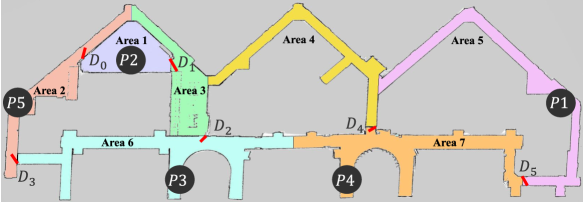
We define seven areas in the map as shown in Figure 2, and each area was manually separated into four subareas (each corresponds to a state). Some of the areas are directly accessible to each other (e.g., Areas 6 and 7), whereas the others are connected through doors (e.g., Areas 1 and 2). We have labeled six doors in the map that our robot can use to enter rooms. All doors are automatic, meaning that, to go through a door, the robot must get close to it, and open it before taking the gothrough action. The real robot needs help from people for door opening actions (printing on its screen “Please help me open the door”), which requires different time durations depending on people’s availability. In simulation, each door is associated with a success-rate distribution, and another distribution over action costs. We tried to give realistic distributions to match the real door’s physical properties (width, location, weight, etc). $D0$, $D2$, and $D5$ are difficult doors, where $D2$ is the most difficult to be opened. $D1$, $D3$, and $D4$ are easy, where $D3$ is the easiest. The simulation environment used in experiments has been created as an extension of OpenAI Gym, a standard platform for RL research (Brockman et al. 2016).

(a) Task $A$: $M_{A}=(P1,P3)$

(b) Task $B$: $M_{B}=(P1,P4)$

(c) Task $C$: $M_{C}=(P2,P3)$

(d) Task $D$: $M_{D}=(P2,P4)$

Figure 3: Average cumulative reward over ten runs (each run includes 2500 episodes), while the robot working on different indoor navigation tasks in simulation. GDQ produced the best performance in all four tasks.

4.1 Simulation Experiment

The agent receives a big reward, $R_{max}$, in successful trials; receives a big penalty, $-R_{max}$, in failure trials; and receives a small cost, $c$, at all other times. In this experiment, $R_{max}=20$, and $c=1$. Our agent tries a random action in probability $\epsilon=0.1$. The learning rate is $\alpha=0.1$, and the discount factor is $\gamma=0.95$. We set a threshold as the maximum number of actions allowed in each episode: not being able to complete a task within 20 actions makes a trial unsuccessful. Each “run” includes $2500$ episodes in a row, and each data point of our figures is an average of over $10$ runs. We have conducted four independent experiments in simulation.

Cumulative Reward

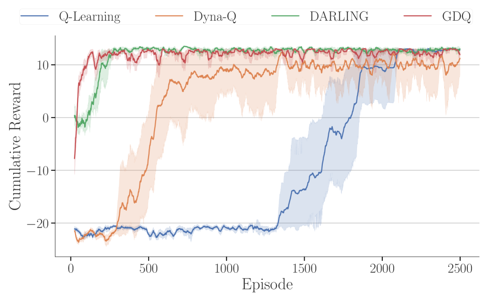
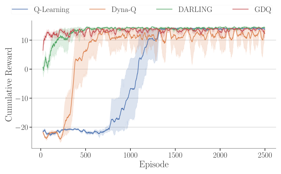
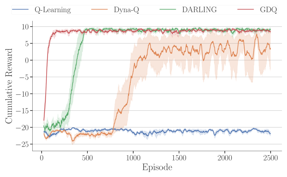
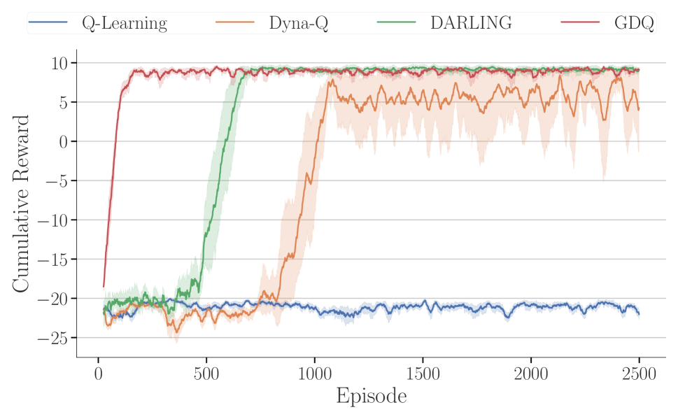
Figures 3 presents the cumulative rewards collected from the robot conducting Tasks $A$, $B$, $C$, and $D$, as well as the tasks’ initial and goal positions. We observe that GDQ performed the best in learning rate in comparison to the four baselines, which supports Hypothesis-I.

Looking into Task-$C$ (bottom-left subfigure), there are the following valid routes that can lead to the goal position while producing different costs and success-rates: $[1\rightarrow 2\rightarrow 6]$, $[1\rightarrow 3\rightarrow 6]$, $[1\rightarrow 3\rightarrow 4\rightarrow 7\rightarrow 6]$, $[1\rightarrow 3\rightarrow 2\rightarrow 6]$, $[1\rightarrow 3\rightarrow 4\rightarrow 5\rightarrow 7\rightarrow 6]$, where each number corresponds to the index of an area. The shortest routes are $[1\rightarrow 2\rightarrow 6]$, and $[1\rightarrow 3\rightarrow 6]$. However, the two routes have doors of $D0$ and $D2$, which are both difficult. In comparison, $[1\rightarrow 3\rightarrow 2\rightarrow 6]$ provides the best trade-off between traveling distance and door difficulty, and is the best solution. GDQ enabled the robot to converge to this solution earlier than all other baseline methods.

Exploration

Aiming to evaluate Hypothesis-II on exploration, we manually provided the ground truth relevance information, where we introduce function $IRR$ that maps a task to a set of irrelevant areas

$$\textit{irrelevant areas}\leftarrow IRR(\textit{task})$$

Back to our testing domain, the irrelevant areas to each task are: $\{1,2,3\}\leftarrow IRR(A)$, $\{1,2,3,6\}\leftarrow IRR(B)$, $\{4,5,7\}\leftarrow IRR(C)$, and $\{2,5\}\leftarrow IRR(D)$

Table 1 shows the results in evaluating the performances in exploration. The bold text indicates the method that produced the least visits, and we say the robot successfully avoids the area using this method. Consider the last four rows that correspond to Task-$D$. We see that GDQ enabled the robot to visit Area-2 for as few as only $37.2$ times, which is much lower than the number of visits required by the other methods (say Q-Learning requires $479.8$ visits), while still produced the best performance in policy quality. This observation is consistent with our prior knowledge that Areas 2 and 5 are less-relevant to Task-$D$. In all four tasks, the robot successfully avoided the irrelevant areas (see the highlighted areas with bold and the listed irrelevant areas in column Task), supporting Hypothesis-II.

(a) Task $C$ to Task $D$

(b) Task $C$ to Task $E$: $M_{E}=(P3,P1)$

Figure 4: The robot conducted two tasks in each experiment to evaluate Hypothesis-III, where the task was changed at the 2500$th$ episode. Average cumulative reward over ten runs (each run includes 5000 episodes), while the robot working on different indoor navigation tasks in simulation. GDQ produced the best performance in the two experiments.

Table 1: This table shows how many times the robot visited each area using four different methods (including GDQ) in conducting the four different tasks. The goal is to show GDQ helps the robot avoid visiting areas that are less-relevant to the given task. Bold text indicates the fewest visits to the less-relevant areas (listed in the “Task” column) among the four methods.

Task	Method	$Area\,1$	$Area\,2$	$Area\,3$	$Area\,4$	$Area\,5$	$Area\,6$	$Area\,7$
	GDQ	$\mathbf{0.0~{}\!(0.0)}$	$14.3~{}\!(0.6)$	$\mathbf{23.8~{}\!(1.1)}$	$944.0~{}\!(42.5)$	$351.9~{}\!(15.9)$	$272.1~{}\!(12.3)$	$613.2~{}\!(26.4)$
Task A	​DARLING​	$1.0~{}\!(0.1)$	$\mathbf{10.0~{}\!(0.5)}$	$27.9~{}\!(1.3)$	$853.9~{}\!(40.8)$	$388.3~{}\!(18.6)$	$260.1~{}\!(12.4)$	$551.6~{}\!(26.4)$
1, 2, 3	Dyna-Q	$12.5~{}\!(0.4)$	$169.6~{}\!(5.5)$	$312.3~{}\!(10.2)$	$1146.2~{}\!(37.4)$	$668.6~{}\!(21.8)$	$200.2~{}\!(6.5)$	$553.1~{}\!(18.6)$
	​​Q-Learning​​	$16.6~{}\!(0.4)$	$394.4~{}\!(9.3)$	$833.3~{}\!(19.7)$	$1435.7~{}\!(34.0)$	$1126.3~{}\!(26.7)$	$93.4~{}\!(2.2)$	$322.2~{}\!(7.6)$
	GDQ	$\mathbf{0.0~{}\!(0.0)}$	$\mathbf{0.5~{}\!(0.0)}$	$\mathbf{3.2~{}\!(0.2)}$	$935.4~{}\!(50.0)$	$352.3~{}\!(18.8)$	$\mathbf{0.0~{}\!(0.0)}$	$581.4~{}\!(31.0)$
Task B	​DARLING​	$0.6~{}\!(0.0)$	$4.7~{}\!(0.3)$	$16.4~{}\!(0.9)$	$839.9~{}\!(47.7)$	$353.3~{}\!(20.1)$	$1.2~{}\!(0.0)$	$545.1~{}\!(31.0)$
1,2,3,6	Dyna-Q	$0.7~{}\!(0.0)$	$50.3~{}\!(1.6)$	$177.0~{}\!(5.6)$	$1372.6~{}\!(43.4)$	$697.5~{}\!(2.2)$	$0.0~{}\!(0.0)$	$861.5~{}\!(27.3)$
	​​Q-Learning​​	$1.0~{}\!(0.0)$	$143.3~{}\!(4.4)$	$459.2~{}\!(14.1)$	$1318.1~{}\!(40.3)$	$981.5~{}\!(30.0)$	$0.0~{}\!(0.0)$	$364.1~{}\!(11.1)$
	GDQ	$\!1025.1~{}\!(31.7)\!$	$984.9~{}\!(30.5)$	$621.8~{}\!(19.3)$	$\mathbf{13.6~{}\!(0.4)}$	$7.5~{}\!(0.2)$	$575.4~{}\!(17.8)$	$2.5~{}\!(0.1)$
Task C	​DARLING​	$\!1343.9~{}\!(40.9)\!$	$832.4~{}\!(25.4)$	$582.1~{}\!(17.7)$	$22.2~{}\!(0.7)$	$\mathbf{6.9~{}\!(0.2)}$	$491.6~{}\!(15.0)$	$3.2~{}\!(0.1)$
4,5,7	Dyna-Q	$\!1943.0~{}\!(43.5)\!$	$854.9~{}\!(19.1)$	$861.9~{}\!(19.3)$	$203.5~{}\!(4.6)$	$101.1~{}\!(2.3)$	$495.3~{}\!(11.1)$	$6.0~{}\!(0.1)$
	​​Q-Learning​​	$\!3146.4~{}\!(59.7)\!$	$472.0~{}\!(9.0)$	$\!1143.0~{}\!(21.7)\!$	$378.4~{}\!(7.2)$	$125.7~{}\!(2.4)$	$0.5~{}\!(0.0)$	$\mathbf{0.6~{}\!(0.0)}$
	GDQ	$\!1031.2~{}\!(31.8)\!$	$\mathbf{37.2~{}\!(1.1)}$	$637.4~{}\!(19.6)$	$943.4~{}\!(29.1)$	$\mathbf{6.7~{}\!(0.2)}$	$20.5~{}\!(0.6)$	$570.0~{}\!(17.6)$
Task D	​DARLING​	$\!1503.7~{}\!(43.5)\!$	$282.1~{}\!(8.2)$	$578.9~{}\!(16.7)$	$553.5~{}\!(16.0)$	$12.3~{}\!(0.4)$	$133.9~{}\!(3.9)$	$394.3~{}\!(11.4)$
2, 5	Dyna-Q	$\!1981.8~{}\!(44.0)\!$	$395.0~{}\!(8.8)$	$882.4~{}\!(19.6)$	$638.3~{}\!(14.2)$	$169.2~{}\!(3.8)$	$98.4~{}\!(2.2)$	$344.0~{}\!(7.6)$
	​​Q-Learning​​	$\!3152.3~{}\!(59.8)\!$	$479.8~{}\!(9.1)$	$\!1140.7~{}\!(21.6)\!$	$374.7~{}\!(7.1)$	$127.4~{}\!(2.4)$	$0.6~{}\!(0.0)$	$0.5~{}\!(0.0)$

Switching Task

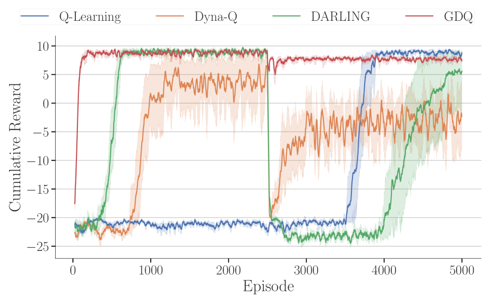
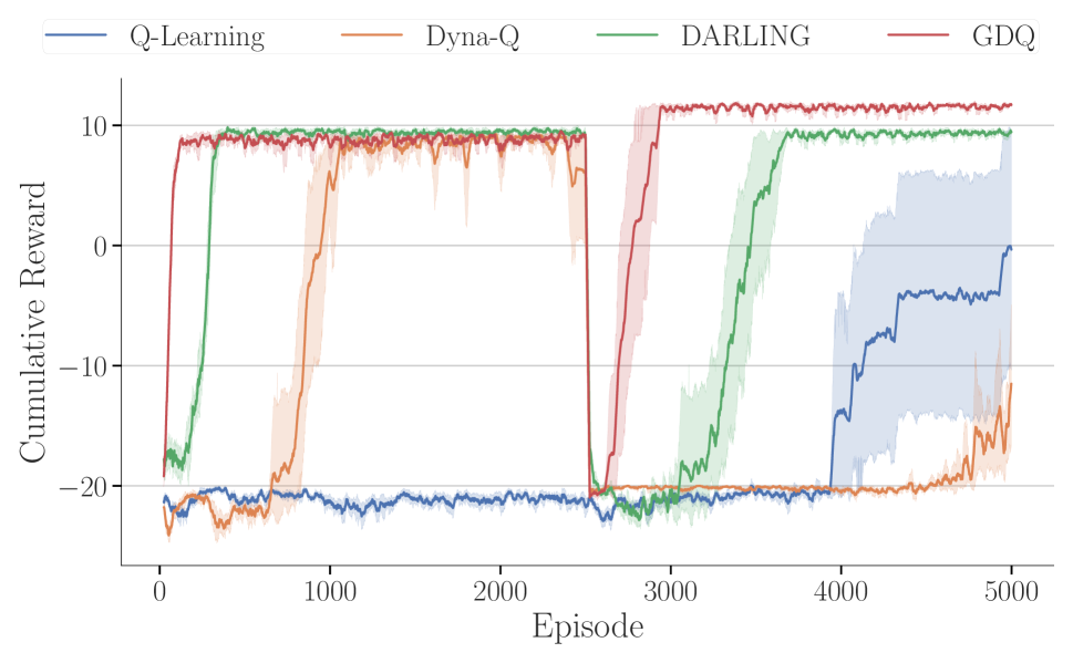
To evaluate Hypothesis III, we studied four scenarios where the robot’s goal is changed after 2500 episodes of training. This experiment was repeated 10 times for computing the averages and standard errors as presented in Figure 4. The two subfigures show the results collected from two cases of task changes. We can see that GDQ can adapt to the task change and learn an optimal policy much faster than the baselines, leveraging the learned task-independent transition function.

4.2 Real Robot Experiment

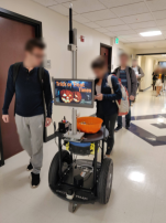
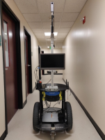
We have conducted experiments using a Segway-based mobile robot platform (Figure 2 on the right). In the real world, the robot has to ask people to help open doors, where the action cost and success rate are noisy and out of our control. We forbade the robot from entering Area-5 in real-world experiments, because it is a long corridor, and navigating through that area takes a very long time. The following parameters are used in the real-robot experiment: $R_{max}=1000$, $\alpha=0.5$, $\gamma=0.95$, and $\epsilon=0.1$. The robot’s task is $M_{X}$ = (P5, P3), referred to as Task-$X$.

Different from simulation experiments, we use time to measure the cost of navigation and door-opening actions (instead of a predefined fixed value). A maximum of $10$ steps is allowed, i.e., if the robot cannot complete Task-$X$ in 10 steps, the corresponding trial will be deemed unsuccessful. We have conducted a total of $30$ trails using the real robot.

Each trial took up to 30 minutes to complete. The Segway-based robot runs out of battery in about five hours, and the experiments were conducted on three consecutive days (5 hours a day, and 15 hours in total). Due to the long time required for each trial (especially in the early learning phase), we only compared GDQ with one baseline.

Figure 5: Task $M_{X}=(P5,P3)$ on a real robot. GDQ enabled the robot to find the optimal path in 22 trials, while Dyna-Q could not find a meaningful solution in 30 trials.

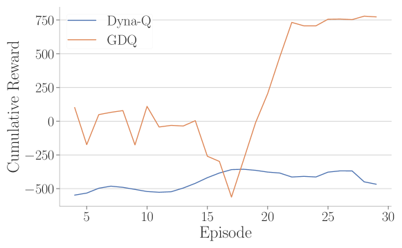
Figure 5 reports the results collected from the real-robot experiment. Looking at the very left of the two curves, the “jump start” of GDQ shows that Algorithm 1 (OptInit) helped the robot successfully avoid the “random” exploration behaviors in the early phase. Once the robot started interacting with the real world, we can see the cumulative reward of GDQ is consistently higher than Dyna-Q, except for only the $17th$ episode. After that, GDQ soon found the optimal solution. In comparison, Dyna-Q could not find a meaningful solution within a total of $30$ episodes.

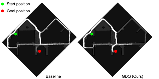
Figure 6 visualizes the frequency of our robot visiting different locations, where a light gray color represents a lower frequency of visits. We see that GDQ enabled the robot to focus more on the left side of the subarea, whereas, using the baseline approach, the robot traversed the right subarea (irrelevant) more. We have generated a video for the demonstration of GDQ’s performance on a real robot.

Figure 6: Heatmaps of a subarea of our office domain for visualizing where the robot visited using the Dyna-Q baseline (Left) and GDQ (Right).

5 Related Work

Automated planning is a branch of automated reasoning research that aims to compute a sequence of actions to accomplish complex tasks. Automated planning methods frequently assume that the agent always gets the desired action outcomes, and unexpected outcomes are handled by plan monitoring and replanning. In comparison, RL methods assume non-deterministic action outcomes, and agents learn from interaction experience. We briefly summarize existing algorithms that leverage automated planning  (Ghallab, Nau, and Traverso 2016) to improve the performance of reinforcement learning methods  (Sutton and Barto 2018) .

Knowledge-based RL:

Researchers have developed algorithms to integrate model-free RL and automated planning to avoid taking unreasonable actions in exploration. Algorithm DARLING is perhaps the earliest work that leverages action preconditions and effects from human knowledge for RL agents to avoid visiting risky or useless state, and has been applied to mobile robot navigation, and grid world domains (Leonetti, Iocchi, and Stone 2016). Researchers have integrated automated planning and Q-learning focusing on non-stationary domains under uncertainties (Ferreira et al. 2017). Those algorithms exploited the flexibility of RL approaches and the accuracy of the declarative knowledge from humans. Other algorithms use action knowledge to improve model-free RL agents’ performance in exploratory behaviors (Ferreira et al. 2019; Zhang et al. 2019). In these works, researchers exploited the pre-designed models for constraining the state or action spaces. In comparison, GDQ (ours) equips the RL agent with the capability of simulating optimistic interaction experience using action knowledge for model learning and policy learning purposes.

Researchers have developed algorithms to use subgoals to guide RL agents. Those subgoals can be learned and represented using non-monotonic logics (Furelos-Blanco et al. 2020), or action languages (Efthymiadis and Kudenko 2013). The main difference from the above-mentioned methods is that GDQ uses model-based RL, whereas they used model-free RL methods that are task-oriented. Our service robotics domain includes potentially many service requests, rendering task-independent methods more suitable. Recently, Zhang and Sridharan researches on leveraging knowledge to improve RL agents’ learning performance.

Hierarchical RL and Automated Planning:

Planning methods have been used to guide the higher level of hierarchical RL methods (Icarte et al. 2018; Yang et al. 2018; Lyu et al. 2019; Jiang et al. 2019a; Illanes et al. 2020; Gordon, Fox, and Farhadi 2019). In those methods, the agents use an action language to compute plans to decompose a complex task into a sequence of subtasks, and each subtask is then implemented by a reinforcement learner. For instance, the work of Jiang et al. (2019a) showed that the introduction of a few milestone positions at the task level can improve mobile robots’ performance in indoor navigation tasks. The work of Icarte et al. (2018) built reward machines using temporal knowledge from domain experts to guide RL agents’ learning behaviors, and also the reward machine can be learned from trial-and-error experiences (Icarte et al. 2019).

The domain knowledge used in those works significantly improved the learning efficiency of RL agents. However, designing the hierarchy is frequently difficult, and many of the hierarchical methods trade optimality for learning efficiency. In comparison, GDQ uses action knowledge that is either publicly available (in our case) or can be easily encoded. Also, the optimistic experience of GDQ generated using action knowledge does not introduce any hard constraints, so GDQ inherits the optimality guarantee from RL algorithms.

Logical Probabilistic Paradigms:

There is the fundamental “logic-probability” gap between model-based RL and automated planning, where model-based RL relies on probabilistic transition systems, and traditionally automated planning does not model quantitative uncertainty. Aiming at bridging this gap, automated planning researchers have used logical-probabilistic paradigms to represent action knowledge, so as to directly reason about probabilistic transitions for model-based RL. For instance, Ng and Petrick (2019) recently developed an algorithm that generates and updates logical-probabilistic action models of automated planning using model-based RL. They used Probabilistic PDDL (Younes and Littman 2004) for action modeling. Alternatively, researchers have developed new knowledge representation paradigms to help agents simultaneously reason with human knowledge and learn the model through interaction with the environment (Wang, Zhang, and Lee 2019; Lu et al. 2020; Sridharan et al. 2019; Veiga et al. 2019; Sanner and Kersting 2010). The above-mentioned methods require the human developer to manually encode logical-probabilistic knowledge, which requires significant professional skills and might soon become infeasible in large domains. In comparison, GDQ requires the minimum amount of action knowledge (widely available in our case), such as “After going through a door, a robot will be on the other side of it (Yang et al. 2014; Jiang et al. 2019b), rendering GDQ more applicable to real-world domains.

6 Conclusions

In this paper, we develop Guided Dyna-Q (GDQ) for bridging the gap between model-based RL, and automated planning. The goal is to help the agent (robot) avoid exploring less-relevant states toward speeding up the learning process. GDQ has been demonstrated and evaluated both in simulation and using a real robot conducting navigation tasks in an indoor office environment. From the experimental results, we see that, using the widely available action knowledge, GDQ performed significantly better than competitive baseline methods from the literature, demonstrating the best performance in learning efficiency.

References

- Bansal et al. (2017) Bansal, S.; Calandra, R.; Chua, K.; Levine, S.; and Tomlin, C. 2017. Mbmf: Model-based priors for model-free reinforcement learning. arXiv preprint arXiv:1709.03153 .
- Brafman and Tennenholtz (2002) Brafman, R. I.; and Tennenholtz, M. 2002. R-max-a general polynomial time algorithm for near-optimal reinforcement learning. Journal of Machine Learning Research .
- Brockman et al. (2016) Brockman, G.; Cheung, V.; Pettersson, L.; Schneider, J.; Schulman, J.; Tang, J.; and Zaremba, W. 2016. Openai gym. arXiv preprint arXiv:1606.01540 .
- Efthymiadis and Kudenko (2013) Efthymiadis, K.; and Kudenko, D. 2013. Using plan-based reward shaping to learn strategies in starcraft: Broodwar. In CIG. IEEE.
- Ferreira et al. (2017) Ferreira, L.; Bianchi, R.; Santos, P.; and de Mantaras, R. L. 2017. Answer set programming for non-stationary Markov decision processes. Applied Intelligence .
- Ferreira et al. (2019) Ferreira, L. A.; dos Santos, T. F.; Bianchi, R. A.; and Santos, P. E. 2019. Solving Safety Problems with Ensemble Reinforcement Learning. In AJCAI, 203–214. Springer.
- Fikes and Nilsson (1971) Fikes, R. E.; and Nilsson, N. J. 1971. STRIPS: A new approach to the application of theorem proving to problem solving. Artif. Intell. 2(3-4): 189–208.
- Furelos-Blanco et al. (2020) Furelos-Blanco, D.; Law, M.; Russo, A.; Broda, K.; and Jonsson, A. 2020. Induction of Subgoal Automata for Reinforcement Learning. In AAAI, 3890–3897.
- Gebser et al. (2011) Gebser, M.; Kaufmann, B.; Kaminski, R.; Ostrowski, M.; Schaub, T.; and Schneider, M. 2011. Potassco: The Potsdam answer set solving collection. Ai Communications .
- Ghallab, Nau, and Traverso (2016) Ghallab, M.; Nau, D.; and Traverso, P. 2016. Automated planning and acting. Cambridge University Press.
- Gordon, Fox, and Farhadi (2019) Gordon, D.; Fox, D.; and Farhadi, A. 2019. What should I do now? marrying reinforcement learning and symbolic planning. arXiv preprint arXiv:1901.01492 .
- Hawes et al. (2017) Hawes, N.; Burbridge, C.; Jovan, F.; Kunze, L.; Lacerda, B.; et al. 2017. The strands project: Long-term autonomy in everyday environments. IEEE Robotics & Automation Magazine 24(3): 146–156.
- Icarte et al. (2018) Icarte, R. T.; Klassen, T.; Valenzano, R.; and McIlraith, S. 2018. Using reward machines for high-level task specification and decomposition in reinforcement learning. In ICML.
- Icarte et al. (2019) Icarte, R. T.; Waldie, E.; Klassen, T.; Valenzano, R.; Castro, M.; and McIlraith, S. 2019. Learning reward machines for partially observable reinforcement learning. NeurIPS .
- Illanes et al. (2020) Illanes, L.; Yan, X.; Icarte, R. T.; and McIlraith, S. A. 2020. Symbolic Plans as High-Level Instructions for Reinforcement Learning. In ICAPS, volume 30, 540–550.
- Jiang et al. (2019a) Jiang, Y.; Yang, F.; Zhang, S.; and Stone, P. 2019a. Task-Motion Planning with Reinforcement Learning for Adaptable Mobile Service Robots. In 2019 IEEE/RSJ International Conference on IROS.
- Jiang et al. (2019b) Jiang, Y.; Zhang, S.; Khandelwal, P.; and Stone, P. 2019b. Task planning in robotics: an empirical comparison of PDDL- and ASP-based systems. Front. Inf. Technol. Electron. Eng. 20(3): 363–373.
- Kaiser et al. (2020) Kaiser, L.; Babaeizadeh, M.; Miłos, P.; Osiński, B.; Campbell, R. H.; Czechowski, K.; et al. 2020. Model Based Reinforcement Learning for Atari. In ICLR.
- Khandelwal et al. (2017) Khandelwal, P.; Zhang, S.; Sinapov, J.; Leonetti, M.; Thomason, J.; Yang, F.; Gori, I.; et al. 2017. Bwibots: A platform for bridging the gap between ai and human–robot interaction research. IJRR .
- Leonetti, Iocchi, and Stone (2016) Leonetti, M.; Iocchi, L.; and Stone, P. 2016. A synthesis of automated planning and reinforcement learning for efficient, robust decision-making. Artif. Intell. .
- Lifschitz (2019) Lifschitz, V. 2019. Answer set programming. Springer.
- Lu et al. (2020) Lu, K.; Zhang, S.; Stone, P.; and Chen, X. 2020. Learning and Reasoning for Robot Dialog and Navigation Tasks. In SIGDIAL.
- Lyu et al. (2019) Lyu, D.; Yang, F.; Liu, B.; and Gustafson, S. 2019. SDRL: Interpretable and Data-Efficient Deep Reinforcement Learning Leveraging Symbolic Planning. In AAAI.
- Mann and Choe (2011) Mann, T. A.; and Choe, Y. 2011. Scaling up reinforcement learning through targeted exploration. In AAAI.
- McDermott et al. (1998) McDermott, D.; Ghallab, M.; Howe, A.; et al. 1998. PDDL-the planning domain definition language.
- Montemerlo et al. (2002) Montemerlo, M.; Thrun, S.; Koller, D.; and Wegbreit, B. 2002. FastSLAM: a factored solution to the simultaneous localization and mapping problem. In AAAI, 593–598.
- Ng and Petrick (2019) Ng, J. H. A.; and Petrick, R. P. A. 2019. Incremental Learning of Planning Actions in Model-Based Reinforcement Learning. In IJCAI.
- Puterman (2014) Puterman, M. L. 2014. Markov Decision Processes.: Discrete Stochastic Dynamic Programming. John Wiley & Sons.
- Racanière et al. (2017) Racanière, S.; Weber, T.; Reichert, D.; Buesing, L.; Guez, A.; Rezende, D. J.; Badia, A. P.; et al. 2017. Imagination-augmented agents for deep reinforcement learning. In Advances in NeurIPS.
- Sanner and Kersting (2010) Sanner, S.; and Kersting, K. 2010. Symbolic dynamic programming for first-order POMDPs. In AAAI.
- Sridharan et al. (2019) Sridharan, M.; Gelfond, M.; Zhang, S.; and Wyatt, J. 2019. REBA: A refinement-based architecture for knowledge representation and reasoning in robotics. JAIR .
- Sutton (1991) Sutton, R. S. 1991. Dyna, an Integrated Architecture for Learning, Planning, and Reacting. SIGART Bull. .
- Sutton and Barto (2018) Sutton, R. S.; and Barto, A. G. 2018. Reinforcement learning: An introduction. MIT press.
- Thrun, Burgard, and Fox (2005) Thrun, S.; Burgard, W.; and Fox, D. 2005. Probabilistic Robotics. MIT Press.
- Veiga et al. (2019) Veiga, T.; Silva, M.; Ventura, R.; and Lima, P. 2019. A hierarchical approach to active semantic mapping using probabilistic logic and information reward POMDPs. In ICAPS.
- Veloso (2018) Veloso, M. M. 2018. The Increasingly Fascinating Opportunity for Human-Robot-AI Interaction: The CoBot Mobile Service Robots. ACM Transactions on HRI .
- Wang, Zhang, and Lee (2019) Wang, Y.; Zhang, S.; and Lee, J. 2019. Bridging Commonsense Reasoning and Probabilistic Planning via a Probabilistic Action Language. Theory and Practice of Logic Programming .
- Yang et al. (2014) Yang, F.; Khandelwal, P.; Leonetti, M.; and Stone, P. H. 2014. Planning in answer set programming while learning action costs for mobile robots. In AAAI-SSS.
- Yang et al. (2018) Yang, F.; Lyu, D.; Liu, B.; and Gustafson, S. 2018. PEORL: Integrating Symbolic Planning and Hierarchical Reinforcement Learning for Robust Decision-Making. In IJCAI.
- Younes and Littman (2004) Younes, H. L.; and Littman, M. L. 2004. PPDDL1. 0: An extension to PDDL for expressing planning domains with probabilistic effects. Techn. Rep. CMU-CS-04-162 2: 99.
- Zhang et al. (2019) Zhang, H.; Gao, Z.; Zhou, Y.; Zhang, H.; Wu, K.; and Lin, F. 2019. Faster and Safer Training by Embedding High-Level Knowledge into Deep Reinforcement Learning. arXiv preprint arXiv:1910.09986 .
- Zhang and Sridharan (2020) Zhang, S.; and Sridharan, M. 2020. A Survey of Knowledge-based Sequential Decision Making under Uncertainty. arXiv preprint arXiv:2008.08548 .