Radio Observations of Magnetic Cataclysmic Variables

Abstract

The NSF’s Karl G. Jansky Very Large Array (VLA) is used to observe 122 magnetic cataclysmic variables (MCVs) during three observing semesters (13B, 15A, and 18A). We report radio detections of 33 stars with fluxes in the range 6–8031 $\mu$Jy. Twenty-eight stars are new radio sources, increasing the number of radio detected MCVs to more that 40. A surprising result is that about three-quarters (24 of 33 stars) of the detections show highly circularly polarized radio emission of short duration, which is characteristic of electron cyclotron maser emission. We argue that this emission originates from the lower corona of the donor star, and not from a region between the two stars. Maser emission enables a more direct estimate of the mean coronal magnetic field of the donor star, which we estimate to be 1–4 kG assuming a magnetic filling factor of 50%. A two-sample Kolmogorov-Smirnov test supports the conclusion that the distribution function of radio detected MCVs with orbital periods between 1.5–5 hours is similar to that of all MCVs. This result implies that rapidly-rotating (P${}_{spin}<10$ days), fully convective stars can sustain strong magnetic dynamos. These results support the model of Taam & Spruit [1989] that the change in angular momentum loss across the fully convective boundary at P${}_{orb}\approx 3$ hours is due to a change in the magnetic field structure of the donor star from a low-order to high-order multipolar field.

1 Introduction

A project was initiated early in 2013 using the NRAO Very Long Baseline Array (VLBA) to perform astrometry of six radio-bright ($>1$ mJy) magnetic cataclysmic variables (MCVs) (namely, BG CMi, AM Her, DQ Her, ST LMi, GK Per, & AR UMa) in an attempt to accurately measure their distances. These observations were carried out in Semesters 13B and 14A. Astrometry requires at least four observations at roughly three month intervals with preferably two observations being at quadrature for best results. Unfortunately, source variability resulted in less than four successful observations per star. As a result, this project was only partially successful. The results of these observations are in preparation. At the same time, a survey was begun using the NSF’s Karl G. Jansky Very Large Array (VLA) to identify new radio-bright MCVs for follow-up VLBA astrometry. Previous to the current study, only eight MCVs were known radio sources; four polars (V834 Cen, AM Her, ST LMi, & AR UMa) and four Intermediate Polars (IPs; AE Aqr, BG CMi, DQ Her, & GK Per). We note that contemporaneous with this study, Coppejans et al. [2015, 2016] observed nine nearby dwarf novae and nova-like CVs and detected eight of them at a flux level of a few tens of $\mu$Jy. The success of the first VLA survey in 2013 was motivation to expand this project to encompass all known MCVs.

The present paper is a status report of this project as of July 2018. Section 2 is a summary of the observations and data analysis of the surveys that have been performed since 2013, with particular emphasis on those during VLA Semesters 13B, 15A and 18A. Section 3 is a summary of the results of these three surveys, including the list of detected sources. The observations and results of the complete survey, including detections and non-detections, will be published in a separate paper. In Section 4, we primarily focus on the circular polarized emission from these sources. We discuss the most likely site of this emission and its implication for the donor star’s mean coronal magnetic field and CV evolution. Our conclusions are given in Section 5.

2 Observations and Data Analysis

For our initial set of VLA observations, we observed 111 MCVs during two observing semesters, 13B and 15A, at primarily three frequencies (C-, X-, and K-bands; 4–6, 8–10, and 20–22 GHz, respectively) at full polarization. A fourth frequency, Q-band (40–44 GHz), was also used for a few observations during Semester 13B. No detections were made at this frequency. For semester 13B, 40 hours of observing time was requested to observe 60 of the optically (B magnitude) brightest, and likely closest, MCVs from the Ritter & Kolb [2003] Catalog of cataclysmic binaries, low-mass X-ray binaries and related objects (Seventh edition); (sp., ed. 7.19) that are north of declination $-40$^∘. An equal number of targets were selected from the polar and IP subclasses in order to avoid biasing the sample toward the brighter IPs. The targets were also chosen to span a wide range of local sidereal time. The observing program allowed about three MCVs to be observed in each one hour scheduling block (SB). Exposures were approximately two minutes per frequency. Each SB was scheduled twice to increase the probability of detecting the MCVs. The VLA scheduled 35 of the 40 hour, resulting in 42 MCVs being observed. For semester 15A, 69 hour of observing time was requested to observe another 69 MCVs in the Ritter & Kolb catalog. Except for one SB, each SB contained two MCVs with each exposure being approximately five minutes per frequency. The VLA scheduled all 69 hour resulting in an additional 69 MCVs being observed. See Barrett et al. [2017] for a detailed discussion of the data analysis and results of these observations.

We have also performed several additional surveys. For Semester 16B, we observed AM Her and AR UMa for 21 hours at C-, X-, & K-bands. An additional 56 hours of time were used to observe another set of 56 MCVs during semesters 17B and 18A; 14 hours during Semester 17B, and 42 hours during Semester 18A. The latter two surveys were only observed using the X-band, which enables longer ($\approx 20$ minutes) exposures on each source. In summary, for the surveys to date, we have obtained 195 out of 199 hours by performing 1 hour filler observations. The data presented in this paper are from Semesters 13B, 15A, and 18A. The data from Semesters 13B and 15A are presented in Barrett et al. [2017], whereas the data from Semester 18A are new. The remaining observations will appear in a series of forthcoming papers.

As discussed in Barrett et al. [2017], all data are calibrated using the VLA CASA automated calibration pipeline. The data from Semesters 13B and 15A use version 4.2.2, and Semester 18A uses version 5.1.2. The clean (ver. 4.2.2) and tclean (ver 5.1.2) algorithms are then used for source detection and flux measurements. Six polarization or Stokes images (sp., I, Q, U, V, RR, and LL, where LL and RR are the left and right polarization channels, resp.) are created for each observation and target. The cleaning is performed in two steps: one for the I, Q, U, and V planes; and one for the RR and LL planes. The Stokes I image is usually best for detecting weakly polarized sources; while the Stokes RR and LL images, for strongly polarized sources. (Henceforth, circular polarization is implied when referring to polarization. No sources show linear polarization.) The size of the image depends on the VLA configuration and observing band. A typical image size for the X band is $10\times 10$ arcseconds. The clean algorithm uses natural weighting, because all sources are assumed to be point sources. The cleaned (model) and residual images are used to measure the source flux and the standard deviation of the noise, respectively. The polarization and its error are calculated from the cleaned and residual polarization images.

3 Results

3.1 Radio Detections

Table 1 is an abbreviated list of detections of 33 MCVS as of July 2018, i.e., from observing semesters 13B, 15A, and 18A. A complete list of detections and upper limits will be given in a forthcoming paper. Columns 1-4 are respectively the GVCS name, MCV subclass, observing semester, and frequency band. The C, X, and K-band frequencies for Semesters 13B and 15A are 4.464–6.512, 7.964–10.012, and 20.060–22.108 GHz; and the X-band frequencies for Semesters 18A are 7.928–12.024 GHz. Columns 5–7 are the Stokes I, and the RR and LL polarization fluxes in $\mu$Jy. The fluxes of the remaining Stokes parameters (Q, U, & V) are omitted. Column 8 is the percentage of circular polarization. Column 9 is the total signal-to-noise (S/N) of the detection. It is the product of the S/N of the Stokes I flux, the circular polarization fluxes, and the PSF-normalized difference of the observed and expected source positions. For highly polarized sources, the S/N of the polarized flux can be much greater than the Stokes I flux and therefore be the major factor in the total S/N. The algorithm for the total S/N and the probability of source misidentification is described by Barrett et al. [2017]. Except for a few sources, most of the observed positions are within a few tenths of an arcsecond of the Gaia position [Gaia Collaboration; Prusti, et al., 2016, Gaia Collaboration; Brown et al., 2018]. For sources having multiple detections at a particular frequency, only the greatest flux is listed. Because these radio sources are highly variable, it was not unusual for the source to be detected in only one of the two observations.

Name	Type	Sem-	Band	Distance		I    Flux		RR Flux		LL Flux		Circ Pol		S/N1
		ester		(arcsec)		($\mu$Jy)		($\mu$Jy)		($\mu$Jy)		(%)
EQ Cet	AM	15A	K	0.78$\pm$	0.30	96$\pm$	30	111$\pm$	55	0$\pm$	55	+100$\pm$	70	11.2
Cas 1	IP	13B	C	1.87$\pm$	2.50	21$\pm$	10	0$\pm$	33	117$\pm$	32	-100$\pm$	39	9.7
FL Cet	AM	18A	X	0.17$\pm$	0.25	11$\pm$	5	24$\pm$	9	0$\pm$	9	+100$\pm$	53	6.6
BS Tri	AM	15A	X	0.07$\pm$	1.00	57$\pm$	9	49$\pm$	16	0$\pm$	15	+100$\pm$	45	23.3
EF Eri	AM	13B	X	0.32$\pm$	1.20	87$\pm$	15	0$\pm$	30	135$\pm$	31	-100$\pm$	30	25.8
UZ For	AM	15A	C	1.46$\pm$	2.50	78$\pm$	9	0$\pm$	25	85$\pm$	26	-100$\pm$	42	39.6
Tau 4	AM?	15A	X	0.22$\pm$	1.00	105$\pm$	32	0$\pm$	72	150$\pm$	74	-100$\pm$	69	8.0
LW Cam	AM	18A	X	0.06$\pm$	0.30	50$\pm$	4	0$\pm$	6	98$\pm$	6	-100$\pm$	9	$>$99.9
VV Pup	AM	13B	X	0.04$\pm$	0.95	79$\pm$	14	82$\pm$	25	0$\pm$	24	+100$\pm$	42	20.4
		13B	K	0.36$\pm$	0.45	49$\pm$	29	103$\pm$	60	47$\pm$	61	+37$\pm$	57	4.5
FR Lyn	AM	18A	X	0.13$\pm$	0.22	28$\pm$	4	12$\pm$	6	38$\pm$	6	-52$\pm$	17	43.3
Hya 1	AM	18A	X	0.04$\pm$	0.23	6$\pm$	6	0$\pm$	8	29$\pm$	8	-100$\pm$	39	7.3
HS0922+1333†	AM	18A	X	0.03$\pm$	0.22	8$\pm$	5	5$\pm$	7	3$\pm$	7	+25$\pm$	100	4.5
WX LMi	AM	15A	C	0.06$\pm$	0.38	73$\pm$	12	49$\pm$	17	26$\pm$	19	+31$\pm$	34	22.8
		15A	X	0.07$\pm$	0.27	52$\pm$	14	33$\pm$	17	48$\pm$	17	-19$\pm$	30	13.4
ST LMi∗	AM	13B	X	0.08$\pm$	0.70	153$\pm$	12	0$\pm$	30	221$\pm$	31	-100$\pm$	20	95.2
AR UMa∗	AM	13B	C	0.23$\pm$	1.30	489$\pm$	16	492$\pm$	25	428$\pm$	28	+7$\pm$	4	$>$99.9
		13B	X	0.19$\pm$	0.78	432$\pm$	14	439$\pm$	24	396$\pm$	24	+5$\pm$	4	$>$99.9
		13B	K	0.16$\pm$	0.34	317$\pm$	30	252$\pm$	45	255$\pm$	45	-1$\pm$	13	79.4
EU UMa	AM	18A	X	0.06$\pm$	0.22	39$\pm$	5	34$\pm$	6	33$\pm$	7	+1$\pm$	14	53.1
V1043 Cen	AM	18A	X	0.16$\pm$	0.60	20$\pm$	5	0$\pm$	7	20$\pm$	8	-100$\pm$	53	11.2
J1503-2207	AM	18A	X	0.03$\pm$	0.45	29$\pm$	5	66$\pm$	7	0$\pm$	6	+100$\pm$	14	55.5
BM CrB	AM	13B	X	0.06$\pm$	0.81	43$\pm$	15	0$\pm$	24	83$\pm$	24	-100$\pm$	41	10.3
MR Ser	AM	13B	C	0.12$\pm$	1.35	239$\pm$	17	371$\pm$	27	0$\pm$	32	+100$\pm$	11	$>$99.9
		13B	X	0.06$\pm$	0.78	116$\pm$	15	221$\pm$	24	0$\pm$	24	+100$\pm$	15	65.2
MQ Dra	AM	18A	X	0.20$\pm$	0.25	17$\pm$	4	25$\pm$	6	0$\pm$	6	+100$\pm$	34	17.4
AP CrB	AM	18A	X	0.11$\pm$	0.30	24$\pm$	4	18$\pm$	6	20$\pm$	6	-5$\pm$	22	27.0
Her 1	AM	15A	K	1.27$\pm$	0.42	48$\pm$	17	106$\pm$	33	0$\pm$	34	+100$\pm$	45	14.2
V1007 Her	AM	15A	X	2.72$\pm$	1.20	38$\pm$	9	75$\pm$	15	0$\pm$	16	+100$\pm$	29	23.3
V1323 Her	IP	15A	C	2.16$\pm$	1.90	43$\pm$	9	80$\pm$	12	0$\pm$	11	+100$\pm$	20	32.2
		15A	X	0.49$\pm$	1.20	23$\pm$	9	0$\pm$	15	53$\pm$	15	-100$\pm$	40	10.0
AM Her∗	AM	13B	C	0.27$\pm$	1.60	88$\pm$	5	57$\pm$	9	84$\pm$	9	-19$\pm$	9	$>$99.9
		13B	X	0.13$\pm$	0.92	192$\pm$	12	176$\pm$	17	171$\pm$	17	+1$\pm$	7	$>$99.9
		13B	K	0.22$\pm$	0.61	476$\pm$	83	172$\pm$	122	440$\pm$	109	-44$\pm$	27	24.7
V603 Aql∗	SH	13B	C	0.13$\pm$	2.90	22$\pm$	3	15$\pm$	6	0$\pm$	6	+100$\pm$	29	35.4
		13B	X	0.16$\pm$	1.70	32$\pm$	7	35$\pm$	12	0$\pm$	12	+100$\pm$	59	13.2
V1432 Aql	AM	18A	X	0.04$\pm$	0.26	15$\pm$	5	21$\pm$	7	0$\pm$	7	+100$\pm$	47	9.3
J1955+0045	AM	18A	X	0.09$\pm$	0.28	79$\pm$	5	70$\pm$	6	73$\pm$	7	-2$\pm$	6	$>$99.9
QQ Vul	AM	13B	K	0.10$\pm$	0.50	92$\pm$	39	0$\pm$	56	134$\pm$	58	-100$\pm$	60	36.9
AE Aqr∗	IP	15A	C	0.01$\pm$	1.39	5123$\pm$	9	5048$\pm$	20	5074$\pm$	20	0$\pm$	1	$>$99.9
		15A	X	0.01$\pm$	0.88	5497$\pm$	11	5462$\pm$	24	5425$\pm$	26	0$\pm$	1	$>$99.9
		15A	K	0.03$\pm$	0.40	8031$\pm$	34	7924$\pm$	54	7881$\pm$	53	0$\pm$	1	$>$99.9
HU Aqr	AM	18A	X	0.25$\pm$	0.23	44$\pm$	13	16$\pm$	13	64$\pm$	13	-60$\pm$	23	18.4
V388 Peg	AM	18A	X	0.04$\pm$	0.23	34$\pm$	5	73$\pm$	6	0$\pm$	6	+100$\pm$	12	86.8

Table 1: List of radio detected MCVs.
¹: The total S/N is the product of the S/N of the relative distance, flux, and polarized flux (see Section 3.1).
^∗: Previously known radio source.
^†: S/N is the product of two detections.

The detection rate from the shorter (2 and 5 minute) exposures in Semesters 13B and 15A is about 16% (19 of 122 stars). It increases to about 33% (14 of 42 stars) for the longer 20 minute exposures in Semester 18A. The detection rate at the C-, X-, and K-band frequencies are 8% (9 of 122 stars), 19% (30 of 142 stars), and 6% (7 of 122 stars), respectively. The fraction of stars showing high polarization in at least one observation or exposure is $\approx 73$% (24 of 33 stars). The number of stars showing little to no ($<10$%) polarization is about 24% (8 of 33) and one star (V1043 Cen) shows high polarization during the first detection and no polarization during the second.

4 Discussion

4.1 Unpolarized Emission

Fourteen of the radio detections show unpolarized continuum emission with a very high brightness temperature. Such emission is characteristic of an incoherent radiative process in an optically thick plasma. The radiation is believed to be mostly gyrosynchrotron emission by mildly relativistic ($1<\gamma<5$) electrons gyrating in a magnetic field. We believe that the source of the few tens of keV to few MeV electrons are magnetic reconnection events in the region between the two stars or near the surface of the late-type donor star.

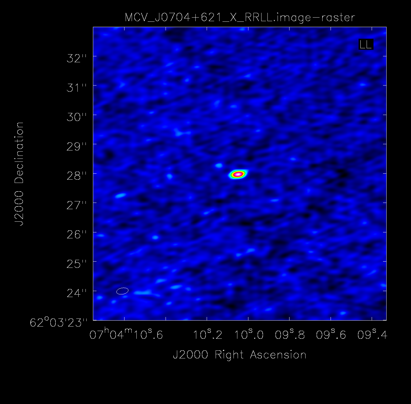
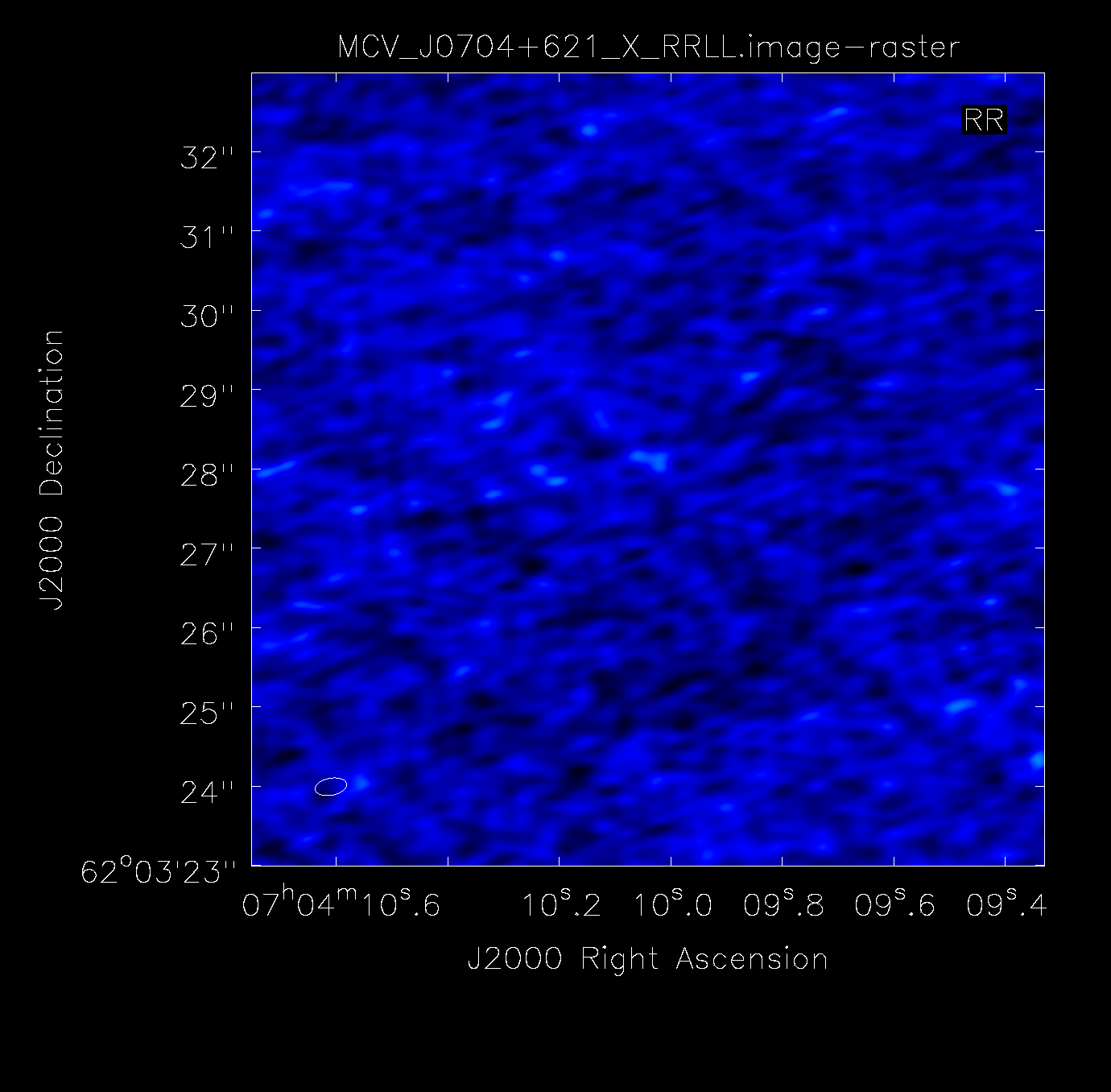
Figure 1: A ten minute exposure of the respective left and right circularly polarized X-band (10 GHz) images of the polar LW Cam showing the highly polarized radio emission.

4.2 Polarized Emission

A surprising result of this survey is that approximately three quarters of the stars show highly polarized emission of short duration ($\sim$few minutes). An example of such emission is the left and right polarized X-band images of the polar LW Cam (see Figure 1). The left image shows an obvious point source, whereas the right does not. High circular polarization requires the presence of a strong magnetic field (B $>100$ G) and, therefore, limits the possible radiation mechanisms to gyromagnetic and electron cyclotron maser emission. (see, e.g., Dulk, Bastian & Chanmugam [1983], Barrett & Chanmugam [1985], Fuerst et al. [1986], Benz & Guedel [1989]. Gyromagnetic emission is often divided into three energy regimes, non-relativistic ($\gamma=1$) cyclotron, mild-relativistic ($\approx 1<\gamma<\approx 5$) gyrosynchrotron, and relativistic ($\gamma>5$) synchrotron emission, where $\gamma=(1-(v/c)^{2})^{-1/2}$. Each of these mechanisms has problems reproducing the characteristics of the observed emission, i.e., high polarization and short duration (see below). Synchrotron radiation can be eliminated because its generates a broad continuous spectrum and polarization of $<40$% [Bjornsson, 2019]. Cyclotron and gyrosynchrotron emission are also unlikely because very specific conditions are needed to produce high polarization. Specifically, the radiation must be emitted along the magnetic field in a relatively homogeneous plasma [Barrett & Chanmugam, 1985]. Any curvature of the magnetic field and changes in plasma density and temperature will significantly decrease the percentage of polarization. Therefore, the most likely cause of the polarized emission is an electron cyclotron maser. Theoretically, the characteristics of maser emission in a constant magnetic field are high polarization ($>80$%), short timescales ($<600$ s), and narrowband emission ($\Delta f/f<0.01$, where f is frequency; see. e.g. Dulk, Bastian & Chanmugam [1983]). The high polarization and short duration are both seen in the roughly ten minute observations of LW Cam and V603 Aql (see below). The absence of narrow band emission is probably due to emission from a broad range of magnetic fields and multiple emission regions.

One mechanism for producing the cyclotron maser is the loss-cone instability. In this scenario, a plasma of relativistic electrons with an isotropic velocity distribution is confined to a magnetic flux tube. The converging magnetic field creates a magnetic mirror causing most of the electrons to be reflected, while the highest energy electrons precipitate out. The loss cone anisotropy causes the index of refraction of the plasma to be negative. The magnetoionic modes of the plasma are then amplified with the extraordinary (x) mode typically growing much faster than the ordinary (o) mode. This mechanism results in highly polarized radiation. Dulk [1985] shows that the growth rate of the x-mode for a typical loss-cone distribution can be quite large ($\sim 10^{7}$ s^-1), which is equivalent to an amplification length of $\approx 10$ m.

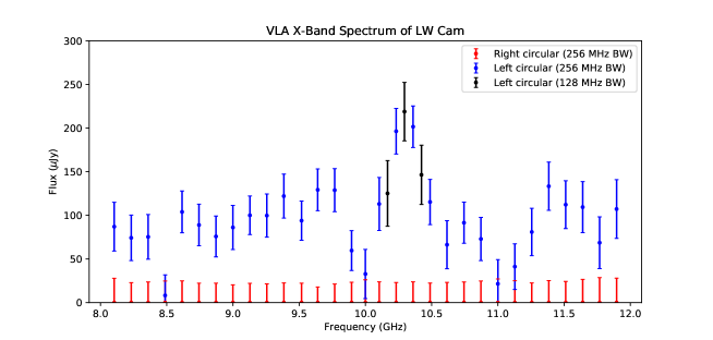
Figure 2: A ten minute X-band (8–12 GHz) spectrum of the polar LW Cam. The blue and red points are the left and right circular polarization channels, respectively. Each point is the average of two adjacent 128 MHz spectral windows in order to reduce the noise. The spectrum suggests the presence of at least one narrowband ($<300$ MHz) emission feature at about 10.295 GHz. The black points show the location of the peak.

Figure 2 is a ten minute X-band (8–12 GHz) spectrum of the polar LW Cam. The blue and red points are the left and right polarization channels, respectively. Each flux value is the average of two adjacent 128 MHz spectral windows (256 MHz bandwidth total), and their flux centroids are within 0.3 arcseconds of the its Gaia position [Gaia Collaboration; Brown et al., 2018]. This averaging of the data reduces the noise, but smoothes the data, which may hide some narrow spectral features. However, the spectrum does suggest the presence of at least one narrowband ($<300$ MHz) emission feature at about 10.295 GHz, which we identify as a pronounced electron maser event. Assuming the maser emission is at the fundamental harmonic, the ambient magnetic field strength of the plasma is determined by the gyrofrequency: f${}_{ce}=2.8$ B MHz, where B is in Gauss. For this particular event, the magnetic field is $\approx$ 3.6 kG. We attribute the remaining polarized emission to be the sum of many smaller maser events with a range of magnetic field strengths.

Given the estimated strength of the magnetic field, there are two possible source locations: in the accretion column and near the surface of the donor star. First, suppose the emission is from the accretion column and the ambient magnetic field is due to the white dwarf. The magnetic field of the white dwarf is usually described by a dipole with $B=2\times 10^{7}r_{9}^{-3}$ G, where $r_{9}$ is the radius of the WD in units of $10^{9}$ cm and the magnetic field of LW Cam is $\approx 20$ MG [Ferrario, De Martino & Gänsicke, 2015]. The emission then originates at a radius of about 18 WD radii, or about a third of the distance from the WD to the inner Lagrangian point at 46 WD radii. The latter radius assumes the WD and donor masses of 0.65 and 0.2 M_⊙, respectively, and an orbital period of 97.3 minutes. For the relevant equations, see equations 2.1b and 2.4c of Warner [1995]. Within the accretion column, the electron number density varies as $n(r)=n_{0}r_{9}^{-5/2}$ cm^-3, where $n_{0}\sim 10^{16}$ cm^-3 at the base of the accretion column [Lamb, Pethick & Pines, 1973]. At 18 WD radii, the electron number density and plasma frequency are $7n_{12}$ cm^-3 and 24 GHz, resp., where $n_{12}=10^{12}$ cm^-3 and f${}_{pe}=9n_{12}^{1/2}$ GHz. A cyclotron maser requires f${}_{ce}>$ f_pe. A condition that is not met within the accretion stream for LW Cam at 8 GHz and is unlikely to be met for other polars at similar frequencies. However, this argument does not exclude maser emission from other low number density ($<10^{12}$ cm^-3) regions within the WD magnetosphere.

In addition, the non-magnetic CV V603 Aql (Nova Aquilae 1918) also shows highly polarized emission (see Table 1). The Ritter & Kolb catalog classifies this CV as a possible IP due to a prominent photometric period, which explains its inclusion in our initial list of targets. However, the photometric period is now associated with a permanent superhump or precession of the accretion disk (see e.g., Mukai & Orio [2005]). If the WD has a magnetic field, it must be weak ($<1$ kG). Otherwise, the Alfvén radius would be at least a few WD radii (for a WD mass of 1.2 M_⊙ and an accretion rate of $1.3\times 10^{17}$ g s^-1) and would noticeably truncate the inner edge of the accretion disk. The far ultraviolet study of V603 Aql by Sion, Godon & Bisol [2015] shows that this is not the case. They do not use truncated accretion disk models to generate their synthetic spectra. The accretion disk is also unlikely to be the site of the polarized emission even when invoking a magneto-rotational instability in the disk in order to increase angular momentum transport out of the inner disk, because the magnetic field of the disk corona in such models is $<1$ kG [Scepi, Dubus & Lesur, 2019].

A more likely site of the polarized emission is in the lower corona of the donor star where the plasma density and frequency are low enough ($n_{e}<10^{12}$ cm^-3 and $f_{pe}<320$ MHz, resp.; Dulk, Bastian & Chanmugam [1983], Dulk [1985]) to allow cyclotron maser emission to escape. The emission site is probably near the footprints of one or more coronal loops with the source of the high energy electrons being from magnetic reconnection events in stellar flares. Although the mean coronal magnetic field of the Sun is low ($<$ few G), because its fractional surface coverage, or filling factor $f$, is very small ($<$1%), the magnetic fields in coronal loops can be $\sim$few kG [Livingston et al., 2006]. In the case of dMe stars, their mean coronal magnetic fields can be $\sim$few kG, because of their larger filling factors ($\sim$50%). For the dMe stars AU Mic, AD Leo, and EV Lac; Saar [1993] estimates mean fields of 2.3 kG, 2.6 kG, and 3.6 KG, respectively. For this survey, the product of the measured field strength in Table 2 and the estimated fillling factor, $fB$, can be used as a rough estimate of the donor star’s mean coronal magnetic field. The data imply mean coronal fields of 1–4 kG, assuming a filling factor of 50%. Higher field strengths are possible, since the current upper bound is constrained by the observing frequency.

Table 2 lists the measured luminosities and magnetic field strengths of the stars listed in Table 1. For stars with measurements at multiple frequencies, only the largest luminosity and highest field strength are listed. Columns 1-4 are the star’s name, the CV subclass, the orbital period in hours, and the star’s distance in parsecs from the Gaia Data Release 2. Column 5 is the flux value that is used to calculate the radio luminosity in column 6. Column 7 is the estimated magnetic field of the emitting region, which we attribute to maser emission. We only list the measured magnetic field strengths for stars having at least one measurement of high polarization. The field strength is calculated using the central frequency and bandwidth of the observation and therefore is only approximate. More accurate estimates of the ambient magnetic field are possible for the brighter stars via spectral analysis and may reveal the presence of multiple emission features and hence, multiple simultaneous emission regions. We intend to provide these results in a forthcoming paper. The range of luminosities is shown as a histogram in Figure 3. Except for AE Aqr, the highest luminosities are probably overestimates caused by inaccurate Gaia distances.

Figure 3: The number of MCVs versus luminosity. The sample is from Table 2.

Name	Type	Period	Distance	Flux	Luminosity∗	B-Field†
		(h)	(pc)	($\mu$Jy)	($10^{24}$ erg s-1)	(Gauss)
EQ Cet	AM	1.5469	285	96	196	7530 $\pm$	365
Cas 1	IP	3.9396	1608	21	292	1960 $\pm$	365
FL Cet	AM	1.4523	319	11	13	3563 $\pm$	730
BS Tri	AM	1.6045	273	57	46	3210 $\pm$	365
EF Eri	AM	1.3503	160	87	24	3210 $\pm$	365
UZ For	AM	2.1087	240	78	24	1960 $\pm$	365
Tau 4	AM?	1.50 ?	210	105	50	3210 $\pm$	365
LW Cam	AM	1.6211	542	50	175	3563 $\pm$	730
VV Pup	AM	1.6739	137	79	16	7530 $\pm$	365
FR Lyn	AM	1.8876	550	28	101
Hya 1	AM	2.3966	441	6	14	3563 $\pm$	730
HS0922+1333	AM	4.0394	163	8	3
WX LMi	AM	2.7821	99	73	4
ST LMi	AM	1.8981	113	153	21	3210 $\pm$	365
AR UMa	AM	1.9320	101	489	27
EU UMa	AM	1.5024	331	39	51
V1043 Cen	AM	4.1902	173	20	7	3563 $\pm$	730
J1503-2207	AM	2.2228	392	29	53	3563 $\pm$	730
BM CrB	AM	1.4040	419	43	81	3210 $\pm$	365
MR Ser	AM	1.8911	132	239	22	3210 $\pm$	365
MQ Dra	AM	4.3912	186	17	7	3563 $\pm$	730
AP CrB	AM	2.5310	209	24	13
Her 1	AM	3.00 ?	1030	48	1281	7530 $\pm$	365
V1007 Her	AM	1.9988	462	38	87	3210 $\pm$	365
V1323 Her	IP	4.4016	2244	43	1163	3210 $\pm$	365
AM Her	AM	3.0942	88	476	93
V603 Aql	SH	3.3168	313	32	34	3210 $\pm$	365
V1432 Aql	AM	3.3656	462	15	38	3563 $\pm$	730
J1955+0045	AM	1.3932	171	79	28
QQ Vul	AM	3.7084	317	92	233	7530 $\pm$	365
AE Aqr	IP	9.8797	91	8031	1673
HU Aqr	AM	2.0836	192	44	19
V388 Peg	AM	3.3751	689	34	193	3563 $\pm$	730

Table 2: List of radio luminosity and donor magnetic field strength.
$*$ Luminosity assumes a 256 MHz bandwidth.
$\dagger$ The magnetic field assumes cyclotron maser emission from the corona of the donor star at the fundamental gyrofrequency, n =1.

Under the assumption that the highly polarized radio emission is from the donor star, these observations have important implications for stellar dynamos in fully convective stars and for CV evolution.

4.3 Cataclysmic Variable Evolution

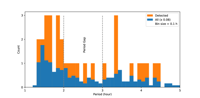
Figure 4: The number of detected MCVs (orange) and all MCVs (blue) versus orbital period. The detected sample is from Table 2. The vertical dashed lines delineate the period gap.

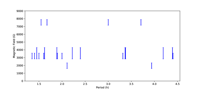
Figure 5: The approximate highest observed magnetic field strength of the electron cyclotron maser emission versus orbital period. The observing frequency is used to estimate the magnetic field strength of the emission region.

The standard model of CV evolution is determined by angular moment loss (AML; Rappaport et al. [1982], Spruit & Ritter [1983]). For P${}_{orb}>3$ hours, magnetic braking is believed to dominate the AML, assuming the magnetic field of the donor stars is $>500$ G. The paucity of CVs with P_orb between 2 and 3 hours was noted by Whyte & Eggleton [1980] and is call the “period gap”. Robinson et al. [1981] suggested that the upper edge of the gap coincides with the orbital period when the donor star becomes fully convective. It has therefore been assumed that magnetic braking is disrupted at P${}_{orb}\approx 3$ hours. At this point, the donor star shrinks and mass transfer ceases. Gravitational radiation then becomes the dominating AML. At about two hours, the orbital radius decreases sufficiently that the donor star overflows its Roche lobe and mass transfer begins again.

The argument for fully convective stars having a weak magnetic field is as follows. Donor stars above the period gap have a tachocline, which is the interface between the radiative core and convective envelope. The tachocline provides a seed magnetic field for the magnetic dynamo in the convective envelope [Spiegel & Zahn, 1992]. Simulations show that strong shearing occurs in the tachocline, causing the local magnetic field to be amplified [Charbonneau, 2014], generating an $\alpha-\Omega$ dynamo, named for the interplay between the cyclonic eddies (the $\alpha$ effect) and the shearing of the field (the $\Omega$ effect). Isolated main-sequence stars later than spectral type M3–M3.5 (M $<3.5$ M_⊙) are predicted to be fully convective and do not possess a tachocline. Therefore, it was conjectured that they cannot sustain a strong dynamo, resulting in a weak magnetic field (B $<100$ G).

Observationally, fully convective stars do display all aspects of stellar activity including optical variability, strong emission lines, and ultraviolet, X-ray, and radio emission (see e.g., Giampapa & Liebert [1986], Stern et al. [1994], Linsky et al. [1995], Hodgkin, et al. [1995], Fleming et al. [1995], Delfosse et al. [1998]). Pevtsov et al. [2003] has shown that the X-ray activity of a late-type star is a good proxy for the surface magnetic flux, and Wright & Drake [2016] have shown that the level of X-ray emission as a function of stellar rotation period is essentially the same for fully convective and partially convective stars. Therefore, these stars must be capable of generating significant magnetic fields. Küker & Rüdiger [1999] studied dynamos in fully convective pre-main-sequence stars using mean field theory. They found that a second order effect, called the $\alpha^{2}$ dynamo, could be excited for moderate rotation rates (P${}_{spin}<10$ d), giving rise to steady, non-axisymmetric mean fields. Local fields as high as 10 kG are generated in some simulations by Browning [2008].

Unlike previous studies that have indirectly inferred a strong magnetic field for the donor star using stellar activity, our observations provide direct measurements of the magnetic field in coronal loops which are used to estimate the mean coronal magnetic fields of the donor stars. We conclude that all polars, and by implication all CVs, have strong magnetic fields throughout their evolution as a result of their rapid rotation. This can be seen in Figure 4, where there is no decrease in the distribution function of radio detected MCVs for P${}_{orb}<3$ hour. A two sample Kolmogorov-Smirnov (K-S) test comparing the two orbital period distributions functions of the radio detected MCVs and all MCVs gives a statistic of 0.129 and a P-value of 0.71. The K-S test result supports the conclusion that the orbital period distribution of radio detected MCVs is the same as that of all MCVs. Figure 5 shows the distribution of the approximate highest observed magnetic field strength with orbital period. Although the data have a strong observational bias because of the small number of detections and the frequency bandwidth of the observations, there is no evidence of a decrease in magnetic field strength with orbital period. This suggests that the magnetic fields of the donor stars for P${}_{orb}<3$ hours are just as strong as they are above 3 hours. This conclusion is supported by recent work on dynamos of fully convective stars.

If the fully convective donor stars in CVs have strong magnetic fields, then another mechanism must be the cause of the CV period gap. One possibility is that there is a change in the structure of the donor star’s magnetic field. Dynamo theory has shown that partially convective stars typically have dipolar or low-order multipolar fields, while fully convective stars have high-order multipoles. Taam & Spruit [1989] have shown low-order multipolar fields are more efficient at AML than high-order multipolar fields. Garraffo et al. [2018b] model CV evolution using the magnetic braking prescription of Garraffo et al. [2018a] and show that it replicates the period gap. However, additional observations and analysis of the radio data are needed to confirm Taam & Spruit’s model. We believe that this explanation is consistent with the study of Knigge, et al. [2011] who have shown that the optimal scaling factors for an empirical model of AML above and below the period gap are: f${}_{MB}=0.66\pm 0.05$ and f${}_{GR}=2.47\pm 0.22$, respectively, where f${}_{MB}=$f${}_{GR}=1$ for the standard model of magnetic braking (MB) and gravitational radiation (GR). A less efficient version of magnetic braking satisfies the need for an additional AML mechanism to that of gravitational radiation for P${}_{orb}<3$ hours.

5 Conclusions

Radio observations of magnetic cataclysmic variables provide a new window for studying the radiation mechanisms and dynamics of these interacting binaries. Under the assumption that the highly circularly polarized emission is due to electron cyclotron maser emission from coronal loops and the donor stars have a high magnetic filling factor, we are able to directly estimate the mean coronal magnetic field strengths to be about 1–4 kG. Although our sample size is limited (33 sources), a two sample K-S test supports our conclusion that the distribution function of donor star magnetic fields is similar to that all MCVs. This result implies that rapidly rotating (P${}_{spin}<10$ d), fully convective stars can sustain a strong magnetic dynamo, and hence, strong coronal magnetic fields. It also suggests that magnetic braking is important throughout the evolution of MCVs, and by implication all CVs, and the change in AML across the fully convective boundary at P${}_{orb}\approx 3$ hours is the result of change in magnetic field structure from low-order to high-order multipolar fields as proposed by Taam & Spruit [1989].

6 Acknowledgements

The National Radio Astronomy Observatory is a facility of the National Science Foundation operated under cooperative agreement by Associated Universities, Inc.

This work has made use of data from the European Space Agency (ESA) mission Gaia (https://www.cosmos.esa.int/gaia), processed by the Gaia Data Processing and Analysis Consortium (DPAC, https://www.cosmos.esa.int/web/gaia/dpac/consortium). Funding for the DPAC has been provided by national institutions, in particular the institutions participating in the Gaia Multilateral Agreement.

The authors wish to thank the editor for her perseverance during this project and to the two anonymous referees for their constructive comments that greatly improved the final version of this paper.

References

- Barrett & Chanmugam [1985] Barrett, P. E. & Chanmugam, G. 1985 ’Cyclotron lines in accreting magnetic white dwarfs with an application to VV Puppis’, ApJ, 298, 743–751
- Barrett et al. [2017] Barrett, P. E., Dieck, C., Beasley, A. J., Singh, K. P., & Mason, P. A. 2017, ’A Jansky VLA Survey of Magnetic Cataclysmic Variables. I. The Data’, AJ, 154, 252–260
- Benz & Guedel [1989] Benz, A. O. & Guedel, M. 1989, ’VLA detection of radio emission from a dwarf nova’, A&A, 218, 137–140
- Bjornsson [2019] Björnsson, C. I. 2019, ’Circular Polarization in Compact Radio Sources: Constraints on Particle Acceleration and Electron-Positron Pairs’, ApJ, 873, 55–67
- Browning [2008] Browning, M. K. 2008, ’Simulations of Dynamo Action in Fully Convective Stars’, ApJ, 676, 1262–1280
- Charbonneau [2014] Charbonneau, P. 2014, ’Solar Dynamo Theory’, ARA&A, 52, 251–290
- Coppejans et al. [2015] Coppejans, D. L., Körding, E. G., Miller-Jones, J. C. A., Rupen, M. P., Knigge, C., Sivakoff, G. R., & Groot, P. J. 2015, ’Novalike cataclysmic variables are significant radio emitters’, MNRAS, 451, 3801–3813
- Coppejans et al. [2016] Coppejans, D. L., Körding, E. G., Miller-Jones, J. C. A., Rupen, M. P., Sivakoff, G. R., Knigge, C., Groot, P. J., Woudt, P. A., Waagen, E. O., & Templeton, M. 2016, ’Dwarf nova-type cataclysmic variable stars are significant radio emitters’, MNRAS, 463, 2229–2241
- Delfosse et al. [1998] Delfosse, X., Forveille, T., Perrier, C. & Mayor, M. 1998, ’Rotation and chromospheric activity in field M dwarfs’, A&A, 331, 581–595
- Dulk, Bastian & Chanmugam [1983] Dulk, G. A., Bastian, T. S., & Chanmugam, G. 1983, ’Radio emission from AM Herculis: the quiescent component and an outburst’, ApJ, 273, 249–254
- Dulk [1985] Dulk. G. A. 1985, ’Radio emission from the sun and stars’, ARA&A, 23, 169–224
- Fuerst et al. [1986] Fuerst, E., Benz, A., Hirth, W., Kiplinger, A. & Geffert, M. 1986, ’Radio emission of cataclysmic variable stars’ A&A, 154, 377–378
- Ferrario, De Martino & Gänsicke [2015] Ferrario, L., de Martino, D., & Gänsicke, B. 2015, ’Magnetic White Dwarfs’, SSRv, 191, 111–169
- Fleming et al. [1995] Fleming, T. A., Schmitt, J. H. M. M. & Giampapa, M. S. 1995, ApJ, ’Correlations of Coronal X-Ray Emission with Activity, Mass, and Age of Nearby K and M Dwarfs’, 450, 401–410
- Gaia Collaboration; Prusti, et al. [2016] Gaia Collaboration; Prusti, T. et al. 2016, ’The Gaia mission’ A&A, 595, 1–36
- Gaia Collaboration; Brown et al. [2018] Gaia Collaboration; Brown, A. G. A. et al. 2018, ’Gaia Data Release 2. Summary of the contents and survey properties’, A&A, 616, 1–22
- Garraffo et al. [2018a] Garraffo, C., Drake, J. J., Dotter, A., Choi, J., Burke, D. J., Moschou, S. P., Alvarado-Gomez, J. D., , Kashyap, V. L., & Cohen, O. 2018, ’The Revolution Revolution: Magnetic Morphology Driven Spin-Down’, ApJ, 862, 90–96
- Garraffo et al. [2018b] Garraffo, C., Drake, J. J., Alvarado-Gomez, S. P., Moschou, S. P. & Cohen, O. 2018, ’The Magnetic Nature of the Cataclysmic Variable Period Gap’, ApJ, 868, 60–65
- Giampapa & Liebert [1986] Giampapa, M. S. & Liebert, J. 1986, ’High-Resolution H alpha Observations of M Dwarf Stars: Implications for Stellar Dynamo Models and Stellar Kinematic Properties at Faint Magnitudes’, ApJ, 305, 784–794
- Hodgkin, et al. [1995] Hodgkin, S. T., Jameson, R. F. & Steele, I. A. 1995, ’Chromospheric and coronal activity of low-mass stars in the Pleiades’, MNRAS, 274, 869–883
- Knigge, et al. [2011] Knigge, C., Baraffe, L. & Patterson, J. 2011, ’The Evolution of Cataclysmic Variables as Revealed by Their Donor Stars’, ApJS, 194, 28–75
- Küker & Rüdiger [1999] Küker, M. & Rüdiger, G. 1999, ’Dynamos in Fully Convective Stars’, ASP Conf Series, 178, 87–96
- Lamb, Pethick & Pines [1973] Lamb, F. K., Pethick, C. J. & Pines, D. 1973, ’A Model for Compact X-Ray Sources: Accretion by Rotating Magnetic Stars’, ApJ, 184, 271–290
- Linsky et al. [1995] Linsky, J. L., Wood, B. E., Brown, A., Giampapa, M. S. & Ambruster, C. 1995, ’Stellar Activity at the End of the Main Sequence: GHRS Observations of the M8 Ve Star VB 10’, ApJ, 455, 670–676
- Livingston et al. [2006] Livingston, W., Harvey, J. W., Malanushenko, O. V., & Webster, L. 2006, ’Sunspots with the strongest magnetic fields’, Sol Phys, 329, 41–68
- Mukai & Orio [2005] Mukai, K. & Orio, M. 2005, ’X-Ray Observations of the Bright Old Nova V603 Aquilae’, ApJ, 622, 602–612
- Pevtsov et al. [2003] Pevtsov, A. A., Fisher, G. H., Acton, L. W., Longcope, D. W., Johns-Kull, C. M., Kankelborg, C. C. & Metcalf, T. R. 2003, ’The Relationship Between X-Ray Radiance and Magnetic Flkux’, ApJ, 598, 1387–1391
- Ritter & Kolb [2003] Ritter, H. & Kolb, U. 2003, ’Catalogue of cataclysmic binaries, low-mass X-ray binaries and related objects (Seventh edition)’, A&A, 404, 301–303
- Rappaport et al. [1982] Rappaport, S., Joss, P. C & Webbink, R. F. 1982, ’The evolution of highly compact binary stellar systems’, ApJ, 254, 616–640
- Robinson et al. [1981] Robinson, E. L., Barker, E. S., Cochran, A. L., Cochran, W. D. & Nather, R. E. 1981, ’MV Lyr: spectrophotometric properties of minimum light: or on MV Lyr off’, ApJ, 251, 611–619
- Saar [1993] Saar, S. H. 1993, ’New Infrared Measurements of Magnetic Fields of Cool Stars’, IAU Symp. 154, ed. D. M. Rabin, J. T. Jefferies, & C. Lindsey, Kluwer Academic Publishers; Dordrecht, 493
- Scepi, Dubus & Lesur [2019] Scepi, N., Dubus, G. & Lesur, G. 2019, ’Magnetic wind-driven accretion in dwarf novae’, A&A, 626, 116–123
- Sion, Godon & Bisol [2015] Sion, E. M., Godon, P. & Bisol, A. 2015, ’Far-ultraviolet Spectroscopy of Old Novae, I. V603 Aql’, AJ, 150, 36–42
- Spiegel & Zahn [1992] Spiegel, E. A. & Zahn, J. P. 1992, ’The solar tachocline’, A&A, 265, 106–114
- Spruit & Ritter [1983] Spruit, H. C. & Ritter, H. 1983, ’Stellar activity and the period gap in cataclysmic variables’, A&A, 124, 267–272
- Stern et al. [1994] Stern, R. A., Schmitt, J. H. M. M., Pye, J. P., Hodgkin, S. T., Stauffer, J. R. & Simon, T. 1994, ’Coronal X-Ray Sources in the Hyades: A 40 Kilosecond ROSAT Pointing’, ApJ, 427, 808–821
- Taam & Spruit [1989] Taam, R. E. & Spruit, H. C. 1989, ’The Disrupted Magnetic Braking Hypothesis and the Period Gap of Cataclysmic Variables’, ApJ, 345, 972–977
- Warner [1995] Warner, B. 1995, ’Cataclysmic Variable Stars’, Cambridge Univ. Press; Cambridge, 27
- Whyte & Eggleton [1980] Whyte, C. A. & Eggleton, P. P. (1980), ’Comments on the evolution and origin of cataclysmic binaries’, MNRAS, 190, 801–823
- Wright & Drake [2016] Wright, N. J. & Drake, J. J. 2016, ’Solar-type dynamo behaviour in fully convective stars without a tachocline’, Nature, 535, 526–528