TESS discovery of a super-Earth and three sub-Neptunes hosted by the bright, Sun-like star HD 108236

Abstract

We report the discovery and validation of four extrasolar planets hosted by the nearby, bright, Sun-like (G3V) star HD 108236 using data from the Transiting Exoplanet Survey Satellite (TESS). We present transit photometry, reconnaissance and precise Doppler spectroscopy as well as high-resolution imaging, to validate the planetary nature of the objects transiting HD 108236, also known as the TESS Object of Interest (TOI) 1233. The innermost planet is a possibly-rocky super-Earth with a period of $3.79523_{-0.00044}^{+0.00047}$ days and has a radius of $1.586\pm 0.098$ $R_{\oplus}$. The outer planets are sub-Neptunes, with potential gaseous envelopes, having radii of $2.068_{-0.091}^{+0.10}$ $R_{\oplus}$, $2.72\pm 0.11$ $R_{\oplus}$, and $3.12_{-0.12}^{+0.13}$ $R_{\oplus}$ and periods of $6.20370_{-0.00052}^{+0.00064}$ days, $14.17555_{-0.0011}^{+0.00099}$ days, and $19.5917_{-0.0020}^{+0.0022}$ days, respectively. With V and K_s magnitudes of 9.2 and 7.6, respectively, the bright host star makes the transiting planets favorable targets for mass measurements and, potentially, for atmospheric characterization via transmission spectroscopy. HD 108236 is the brightest Sun-like star in the visual (V) band known to host four or more transiting exoplanets. The discovered planets span a broad range of planetary radii and equilibrium temperatures, and share a common history of insolation from a Sun-like star ($R_{\star}=0.888\pm 0.017$ R_⊙, $T_{\rm eff}=5730\pm 50$ K), making HD 108236 an exciting, opportune cosmic laboratory for testing models of planet formation and evolution.

1 Introduction

As the number and diversity of the known exoplanets continues to grow, we are gaining a better perspective on our own Solar System. Based on the discovery of more than 4,000 exoplanets to date (Akeson et al., 2013), two common types of exoplanets are the larger analogs of the Earth (super-Earths) and smaller analogs of Neptune (sub-Neptunes) (Fressin et al., 2013; Fulton et al., 2017). Their wide range of orbital architectures and atmospheric properties (Kite et al., 2020; Rein, 2012) motivate further investigation of these small exoplanets in order to accurately characterize their demographic properties.

Transiting exoplanets hosted by bright stars enable detailed characterization such as measurements of radius, mass, bulk composition and atmospheric properties. Furthermore, multiplanetary systems offer laboratories to study how planet formation, evolution and habitability depend on amount of insolation, while controlling for the age and stellar type (Pu & Wu, 2015; Weiss et al., 2018a, b).

The Transiting Exoplanet Survey Satellite (TESS) (Ricker et al., 2014) is a spaceborne NASA mission launched in 2018 to survey the sky for transiting exoplanets around nearby and bright stars. It builds on the legacy of the NASA’s Kepler space telescope (Borucki et al., 2010) launched in 2009, which was the first exoplanet mission to perform a large statistical survey of transiting exoplanets. One of the goals of the TESS mission is to discover 50 exoplanets with radii smaller than 4$R_{\earth}$ and coordinate their mass measurements via precise high-resolution spectroscopic follow-up. This will enable accurate inferences about the bulk composition and atmospheric characterization of small exoplanets.

In this work, we present the discovery and validation of four exoplanets hosted by HD 108236, also identified as the TESS Object of Interest (TOI) 1233. We use the TESS data in sectors 10 and 11 (i.e., UT 26 March 2019 to UT 21 May 2019) as well as ground-based follow-up data to validate the planetary nature of the transits detected in the TESS data and precisely determine the properties of the planets and their host star.

HD 108236 is the brightest Sun-like (G-type) star and one of the brightest stars on the sky to host at least four transiting planets. This makes it an especially useful system for comparative studies of the formation and evolution of its transiting planets in the future. Furthermore, its planets are favorable targets for atmospheric characterization via transmission spectroscopy. With a super-Earth and three sub-Neptunes, the HD 108236 system constitutes a major contribution to the mission goal of TESS. HD 108236 is also the first multiplanetary system delivered by TESS with four validated transiting planets.

This paper is organized as follows. In Section 2, we characterize the host star HD 108236. In Section 3, we present the data collected on the system to discover and validate the planets. We then characterize the planets in Section 4, discuss our results and conclude in Section 5.

2 Stellar characterization

Characterization of an exoplanet, i.e., determination of its mass, $M_{\rm p}$, radius, $R_{\rm p}$, and equilibrium temperature, $T_{\rm eq}$, requires determination of the same properties of its host star. Therefore, we first study and characterize the host star to estimate its radius, $R_{\star}$, mass, $M_{\star}$, and effective temperature, $T_{\rm eff}$, as well as its surface gravity, $\log g$, metallicity, [Fe/H], sky-projected rotational velocity, $v\sin i_{\star}$, and spectroscopic class.

HD 108236 is a bright main-sequence star with a TESS magnitude of 8.65 in the Southern Ecliptic Hemisphere, falling in the Centaurus constellation with a right ascension and declination of 12:26:17.78 -51:21:46.99 (186.574063^∘ -51.363052^∘). Having a parallax of $15.45\pm 0.05$ milli arcsecond (mas) as measured by the Gaia telescope in its Data Release 2 (DR2) (Gaia Collaboration et al., 2018; Bailer-Jones et al., 2018), the host star is 64.6 $\pm$ 0.2 parsecs away. Based on the same Gaia DR2 catalog, it has a proper motion of $-70.43\pm 0.06$ and $-49.87\pm 0.04$ mas per year along right ascension and declination, respectively, and a velocity along our line of sight of $16.78\pm 0.02$ km s^-1. Although we will be referring to the star as HD 108236 throughout this work, some other designations for the target are TIC 260647166, TOI 1233, and HIP 60689.

Table 1: Stellar Information

Identifying Information

Name	TOI 1233, HD 108236
TIC ID	260647166

Parameter

Value

Reference

Astrometric Properties

Right Ascension [∘]	186.574063	Gaia DR2
Declination [∘]	-51.363052	Gaia DR2
$\mu_{\alpha}$ [mas yr-1]	-70.43 $\pm$ 0.06	Gaia DR2
$\mu_{\delta}$ [mas yr-1]	-49.87 $\pm$ 0.04	Gaia DR2
Distance [pc]	64.6 $\pm$ 0.2	TIC v8
RV [km s-1]	$16.78\pm 0.02$ km s-1	Gaia DR2

Photometric Properties

TESS [mag]	8.6522 $\pm$ 0.006	TIC v8
B [mag]	9.89 $\pm$ 0.02	TIC v8
V [mag]	9.25 $\pm$ 0.01	TIC v8
BT [mag]	10.04 $\pm$ 0.02	Tycho-2
VT [mag]	9.313 $\pm$ 0.014	Tycho-2
Gaia [mag]	9.08745 $\pm$ 0.0002	Gaia DR2
Gaia${}_{\text{BP}}$ [mag]	9.43555 $\pm$ 0.000737	Gaia DR2
Gaia${}_{\text{RP}}$ [mag]	8.60563 $\pm$ 0.000643	Gaia DR2
J [mag]	8.046 $\pm$ 0.024	2MASS
H [mag]	7.703 $\pm$ 0.029	2MASS
K${}_{\text{s}}$ [mag]	7.637 $\pm$ 0.031	2MASS
WISE 3.4 [mag]	7.613 $\pm$ 0.029	WISE
WISE 4.6 [mag]	7.673 $\pm$ 0.021	WISE
WISE 12 [mag]	7.638 $\pm$ 0.017	WISE
WISE 22 [mag]	7.51 $\pm$ 0.098	WISE

In the table, mas stands for milli arcseconds. We use the following references: TESS Input Catalog version 8 (TICv8) (Stassun et al., 2019), Gaia DR2 (Gaia Collaboration et al., 2018), Tycho-2 (Høg et al., 2000), 2MASS (Cutri et al., 2003), and WISE (Wright et al., 2010).

Since photometric transit observations only probe the planet-to-star radius ratio, the stellar radius needs to be determined precisely in order to infer the radii of the transiting planets. The stellar radius can be inferred using two independent methods. First, a high-resolution spectrum of the star can be used to derive the stellar parameters, by fitting it with a model spectrum obtained by linearly interpolating a library of template spectra (Coelho et al., 2005). The resulting effective temperature and the distance to the star then yield the stellar radius via the Stefan-Boltzmann law. We used this method to characterize the star based on the high-resolution spectrum described in Section 3.4.1, obtaining the stellar radius and effective temperature as $0.894\pm 0.022\,R_{\odot}$ and $5618\pm 100$ K, respectively.

An independent method of inferring the effective temperature and radius of the host star is to model its brightness across broad bands over a larger wavelength range, known as the spectral energy distribution (SED). This yields a semi-empirical determination of the stellar radius as well as independent constraints on stellar evolution model parameters such as the stellar mass, metallicity and age. Towards this purpose, we used the broad-band photometric magnitudes of HD 108236 provided in Table 1 to model the stellar SED of HD 108236 following the methodology described in Stassun & Torres (2016); Stassun et al. (2017, 2018). To constrain the distance to the star, we used the Gaia DR2 parallaxes, adjusted by 82 $\mu$as to account for the systematic offset reported by Stassun & Torres (2018). We retrieved the $B_{\rm T}$ and $V_{\rm T}$ magnitudes from Tycho-2, the Strömgren $ubvy$ magnitudes from Paunzen (2015), the $JHK_{\rm S}$ magnitudes from 2MASS (Skrutskie et al., 2006; Cutri et al., 2003), the W1, W2, W3, and W4 magnitudes from WISE (Wright et al., 2010), and the $G$, $G_{\rm BP}$, and $G_{\rm RP}$ magnitudes from Gaia (Gaia Collaboration et al., 2018; Bailer-Jones et al., 2018). Together, the available photometry spans the full stellar SED over the wavelength range 0.35-22 $\mu$m as shown Figure 1.

We performed a fit using Kurucz stellar atmosphere models (Castelli & Kurucz, 2003), with the effective temperature, $T_{\rm eff}$, metallicity, [Fe/H], and surface gravity, $\log g$, adopted from the TIC (Stassun et al., 2019) as initial guesses. The only additional free parameter was the extinction ($A_{\rm V}$), which we restricted to be less than or equal to the maximum line-of-sight value from the dust maps of Schlegel et al. (1998). The resulting fit is excellent (Figure 1) with a reduced $\chi^{2}$ of 2.3 and best-fit $A_{\rm V}=0.04\pm 0.04$, $T_{\rm eff}=5730\pm 50$ K, $\log g=4.5\pm 0.5$, and [Fe/H] = $-0.3\pm 0.5$. Integrating the (unreddened) model SED gives the bolometric flux at Earth, $F_{\rm bol}=5.881\pm 0.068\times 10^{-9}$  erg s^-1 cm^-2. Taking the $F_{\rm bol}$ and $T_{\rm eff}$ together with the Gaia DR2 parallax gives the stellar radius, $R_{\star}=0.888\pm 0.017\,R_{\odot}$. Finally, we can use the empirical relations of Torres et al. (2010) and a 6% error from the empirical relation itself to estimate the stellar mass, $M_{\star}=0.97\pm 0.06\,M_{\odot}$; this, in turn, together with the stellar radius provides an empirical estimate of the mean stellar density, $\rho_{\star}=1.94\pm 0.16$ g cm^-3. Based on these properties, the spectral type of HD 108236 can be assigned as G3V (Pecaut & Mamajek, 2013).

In an alternative, isochrone-dependent approach, we also used EXOFASTv2 (Eastman et al., 2019) to constrain the stellar parameters. We relied on the observed SED and the MESA isochrones and stellar tracks (Dotter, 2016; Choi et al., 2016). This approach forces the inference to match a theoretical star based on stellar evolution models. We imposed Gaussian priors on the Gaia DR2 parallax. We added 82 $\mu$as to the reported value and 33 $\mu$as in quadrature to the reported error, following the recommendation of Stassun & Torres (2018). We also imposed an upper limit on the extinction of 0.65 using the dust map of Schlafly & Finkbeiner (2011). In addition, we applied Gaussian priors on $T_{\rm eff}$ and [Fe/H] from the analysis of the high-resolution spectrum described in Section 3.4.1.

The derived stellar parameters from all approaches are summarized in Table 2. When characterizing the transiting planets in the remaining of this paper, we use the stellar radius and the effective temperature of $0.888\pm 0.017$ R_☉ and $5730\pm 50$ K, as inferred from the isochrone-independent approach based on the SED.

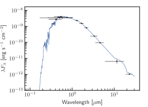
Figure 1: The SED of HD 108236. Black symbols and their vertical error bars represent the photometric measurements that were previously available on the system. The horizontal bars represent the effective width of the passband. Overplotted with the blue line is our best-fit Kurucz atmosphere model, allowing us to characterize the star.

Table 2: Stellar Characterization. Different methods yield consistent models of the host star. The difference between our adopted stellar parameters (i.e., based on an isochrone-independent model of the broad-band photometry) and those of the EXOFAST results can be attributed to the tight isochrone priors of the latter. The difference with the NRES results is largely due to the differences in the information content of broad-band photometry and high-resolution spectra.

Parameter

Value

High-resolution spectroscopy

CHIRON

$T_{\text{eff}}\text{ [K]}$	5638
log [g]	4.39
[Fe/H]	-0.22
$v$sin$i$ [km s-1]	$<$4.7 (95% CL)

LCO/NRES

$T_{\text{eff}}\text{ [K]}$	5618 $\pm$ 100
log [g]	4.6 $\pm$ 0.1
[Fe/H]	-0.26 $\pm$ 0.06
$v$sin$i$ [km s-1]	$<$ 2 (95% CL)
M∗ [M☉]	0.853 $\pm$ 0.047
R∗ [R☉]	0.894 $\pm$ 0.022

Broad-band photometry

Isochrone-independent

$T_{\text{eff}}\text{ [K]}$	5730 $\pm$ 50
log [g]	4.5 $\pm$ 0.5
[Fe/H]	-0.3 $\pm$ 0.5
$A_{\text{v}}$	0.04 $\pm$ 0.04
$F_{\text{bol}}$ [erg s-1 cm-2]	5.881 $\pm$ 0.068 $\times$ 10-9
M∗ [M☉]	0.97 $\pm$ 0.06
R∗ [R☉]	0.888 $\pm$ 0.017
$\rho_{*}$ [g cm-3]	1.94 $\pm$ 0.16

Isochrone-dependent approach via EXOFASTv2

$T_{\text{eff}}\text{ [K]}$	5721 $\pm$ 60
log [g]	4.492 $\pm$ 0.032
[Fe/H]	-0.253 $\pm$ 0.062
Age Gyr	5.8 $\pm$ 4.1
$A_{\text{v}}$	0.04 $\pm$ 0.04
$L_{*}$ [L☉]	0.747 $\pm$ 0.03
M∗ [M☉]	0.877 $\pm$ 0.05
R∗ [R☉]	0.88 $\pm$ 0.017
$\rho_{*}$ [g cm-3]	1.82 $\pm$ 0.15

CL stands for confidence level.

3 Discovery and validation of planets hosted by HD 108236

In this section, we will describe the detection of transit signals consistent with transiting planets hosted by HD 108236 and the follow-up data we collected to rule out alternative hypotheses. Table 3 summarizes the observations we carried out using the resources of the TESS Follow-up Observing Program (TFOP) to validate the planetary origin of the transits and characterize the planets and their host star. The subgroups of TFOP involved in this program were ground-based photometry (SG1), reconnaissance spectroscopy (SG2), high-resolution imaging (SG3), and precise Doppler spectroscopy (SG4).

Table 3: Observations conducted as part of the follow-up of HD 108236 after the detection of transits by TESS.

Date	Telescope/Instrument
Imaging
2020-01-14	Gemini/Zorro
2020-03-12
2020-01-07	SOAR/HRCam
Reconnaissance Spectroscopy
2020-01-28
2020-01-24
2019-08-03	SMARTS/CHIRON
2019-07-04
2019-07-02
2019-06-12	LCOGT/NRES
2019-06-23
Precise Doppler spectroscopy
2019-07-12
2019-07-15
2019-07-16
2019-07-18
2019-07-20
2019-08-08	Magellan II/PFS
2019-08-09
2019-08-11
2019-08-13
2019-08-17
2019-08-20
2019-08-21

Photometric
Date	Telescope	Instrument	TOI
2020-03-17	LCOGT-CTIO	Sinistro	1233.01*
2020-03-17	MEarth-South	Apogee	1233.01
2020-03-11	LCOGT-CTIO	Sinistro	1233.03
2020-03-11	LCOGT-CTIO	Sinistro	1233.02
2020-03-11	MEarth-South	Apogee	1233.02
2020-03-03	MEarth-South	Apogee	1233.01
2020-03-02	LCOGT-SAAO	Sinistro	1233.01
2020-02-02	LCOGT-SAAO	Sinistro	1233.02
2020-01-31	LCOGT-SAAO	Sinistro	1233.03
2020-01-11	LCOGT-SAAO	Sinistro	1233.04
2020-01-11	LCOGT-CTIO	Sinistro	1233.02

A * in the last column denotes a tentative detection of a transit on target.

3.1 TESS

TESS is a spaceborne telescope with four cameras, each with four Charge-Coupled Devices (CCDs) with the primary mission of discovering small planets hosted by bright stars, enabled by its high-precision photometric capability in space (Ricker et al., 2014). The Science Processing Operations Center (SPOC) pipeline (Jenkins et al., 2016) regularly calibrates and reduces TESS data, delivering Simple Aperture Photometry (SAP) (Twicken et al., 2010; Morris et al., 2017) light curves as well as Presearch Data Conditioning (PDC) (Stumpe et al., 2012; Smith et al., 2012; Stumpe et al., 2014) light curves that are corrected for systematics. Then, it searches for periodic transits in the resulting light curves using the Transiting Planet Search (TPS) (Jenkins, 2002; Jenkins et al., 2017) to search for planets. Unlike the Box Least Squares (BLS) (Kovács et al., 2002), which also searches for transit-like pulse trains while not taking into account the correlation structure of noise, TPS employs a noise-compensating matched filter which jointly characterizes the correlation structure of the observation noise while searching for periodic transits. Finally, it delivers the statistically significant candidates as Threshold Crossing Events (TCEs). As members of the TOI working group, we regularly classify these TCEs as planet candidates and false positives. When vetting TCEs as planet candidates, we use the SPOC validation tests (Twicken et al., 2018; Li et al., 2019) such as:

1. the eclipsing binary discrimination test to detect the presence of secondary eclipses and compare the depths of odd and even transits to rule out inconsistencies,

2. the centroid offset test to determine if the centroid of the difference (i.e., out-of-transit minus in-transit) image is statistically consistent with the location of the target star,

3. a statistical bootstrap test to estimate the false positive probability of the TCE when compared to other transit-like features in the light curve, and

4. an optical ghost diagnostic test to rule out false positive hypotheses such as instrumental noise, scattered or blended light, based on the correlations between the model transit and light curves derived from the core photometric aperture and a surrounding halo.

3.2 Discovery of periodic transits consistent with planetary origin

HD 108236 was among the list of targets observed by TESS with a cadence of 2 minutes and also included in the TESS Guest Investigator (GI) Cycle I proposal (G011250, PI: Walter, Frederick). It was observed by TESS Camera 2, CCD 2 during Sector 10 (UT 26 March 2019 - 22 April 2019) and TESS Camera 1, CCD1 during Sector 11 (UT 22 April 2019 - 21 May 2019). The TESS data were processed by the SPOC pipeline. Then, Sector 10 and 11 TESS data and derived products such as the SAP and PDC light curves including that of HD 108236 were made public on 01 June 2019 (data release 14) and 17 June 2019 (data release 16), respectively.

The first detection of a TCE consistent with a planetary origin from HD 108236 was obtained in Sector 10 TESS data. The TCE had a period of 14.178 days. However, the light curve also had other transit-like features unrelated to the detected TCE, which promoted HD 108236 to a potentially high-priority, multiplanetary system candidate. Sector 11 TESS data triggered three TCEs one of which had the same period as that from Sector 10. However, the transits of the other TCEs had inconsistent depths. These initial TCEs from individual sectors were vetted as planet candidates with the expectation that a joint TPS analysis of two sectors of TESS data would resolve the ambiguities on the multiplicity and periods of the planet candidates. The multi-sector data analysis at the end of Sector 13 resulted in the detection of four TCEs with periods 14.18, 19.59, 6.20, and 3.80 days and Signal to Noise Ratios (SNRs) 15.3, 16.2, 11.4, and 8.7, respectively. The PDC light curve of HD 108236 from these two sectors is shown in Figure 2. Subsequently, we released alerts on these four TCEs (i.e., TOI 1233.01, TOI 1233.02, TOI 1233.03, and TOI 1233.04) with planet candidate dispositions on 26 August 2019. For the moment, we will refer to these TCEs that have been vetted as planet candidates using the TOI designations.

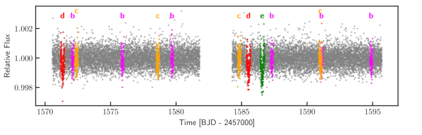
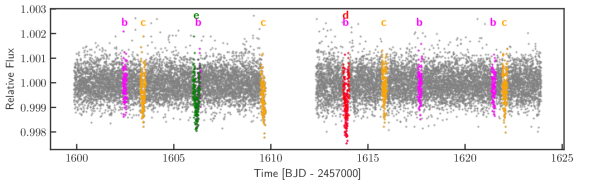
Figure 2: The normalized light curve of HD 108236 measured by TESS, reduced by the PDC pipeline, and detrended by our pipeline, shown with gray points. The top and bottom panels show the Sector 10 and 11 data, respectively. The data show stellar variability, especially in Sector 11, which is taken into account for both Sectors by our red noise model as discussed in Section 3.9. Magenta, orange, red and green colors highlight the transits of the discovered planets b, c, d, and e. Throughout the paper we use the same color scheme to denote the planets.

3.3 Vetting of the planet candidates

Time-series photometry of a source is inferred from photoelectrons counted in a grid of pixels on the focal plane. The finite Point Spread Function (PSF) causes nearby sources to be blended. The focus-limited PSF (full width at half maximum of $\sim 1--2$ pixel) and the large pixel size ($\sim$ 21″) of TESS imply that the resulting time-series photometry of a given target will often have contamination from nearby sources.

Blended light from nearby sources can decrease the depth, $\delta$, of a transit by

$$\delta^{\prime}=\Big{(}1-\dfrac{F_{\rm B}}{F_{\rm T}+F_{\rm B}}\Big{)}\delta=(1-D)\delta=(1-\dfrac{f}{1+f})\delta$$ (1)

where $\delta^{\prime}$ is the diluted transit depth, $F_{\rm B}$ and $F_{\rm T}$ are the fluxes of the blended and target source, respectively. Here, $D$ is dilution, and $f\equiv F_{\rm B}/F_{\rm T}$ is the flux ratio of the blended and target objects. The SPOC pipeline corrects the PDC light curves for this dilution of the transits.

The TESS image of HD 108236 from Sector 10 is shown in Figure 3 along with several archival images of the target including the Science and Engineering Research Council (SERC) J image taken in 1979, SERC-I image taken in 1983 and the Anglo-Australian Observatory Second Epoch Survey (AAO-SES) image taken in 1994. The apertures that are used to extract the TESS light curves are also shown for Sector 10 (red) and 11 (purple). Some of the relatively bright neighbors of HD 108236 are TIC 260647148, 260647113, 260647110, and 260647155 that are 77, 95, 108, and 122″away and have TESS magnitudes of 13.89, 13.73, 12.94, and 11.67, respectively. Due to the large aperture used to collect light from the bright target HD 108236, the total flux from blended sources is roughly $f=1.2\%$ of the photons coming from HD 108236.

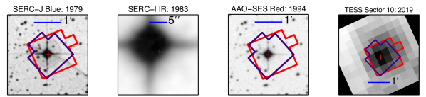
Figure 3: The archival and TESS images of HD 108236. The TESS image is from Sector 10 taken during 2019. Overplotted on the TESS image are the two apertures that are used to extract the light curves during Sector 10 (red) and 11 (purple).

Detection of periodic transits in photometric time-series data can be due to any of the following:

• An instrumental (systematic) effect,

• The primary (i.e., brightest) star being eclipsed by a companion star (i.e., eclipsing binary),

• A foreground or background star (i.e., gravitationally not associated with the target) aligned with the target being eclipsed by a stellar companion or transited by a planet,

• The primary or one of the fainter (secondary) stars in a hierarchical multiple star system eclipsing each other or being transited by a planet,

• A nearby star (i.e., gravitationally not associated with the target) being eclipsed by a stellar companion or transited by a planet,

• A star being transited by a planet.

Therefore, we individually considered and ruled out the alternative hypotheses in order to ensure that the planetary classification for the origin of the detected transits was not a false positive.

The first false-positive hypothesis was that the transits could be due to an instrumental effect. The orbital periods of TOI 1233.03 and TOI 1233.04 were close to the multiples of the momentum dump period, which occurred every 3.125 days for Sectors 10 and 11, according to the TESS Data Release Notes. However, the detected transits did not fall near the momentum dumps. In addition, the transit shapes were inconsistent with that of the typical momentum dump artifact (i.e., sudden drop followed by a gradual rise). The difference images also did not show any evidence of scattered light in the vicinity of HD 108236 during the observations of interest. Furthermore, there were many individual transits detected, which made it extremely unlikely that they were produced by unrelated systematic events. This ruled out the instrumental origin of the detected transits.

The transit model fit performed by the SPOC pipeline on the TESS data indicated that the transit was not grazing and that the depth and shape of the transits were consistent with being of planetary nature. This was also confirmed later with our transit model as discussed in Section 3.9. The SPOC data validation also showed that the apparent positions of the TCEs were all within 1 pixel of HD 108236. Nevertheless, the periodic dimming could be due to any of the sufficiently bright sources in the aperture, since transits or eclipses from nearby or physically associated companion stars could be blending into the aperture. In general, dynamical measurements such as Transit Timing Variations (TTVs) could break this degeneracy. However, the small number of transits and the limited baseline ($\sim$ 60 days) of the detection data did not yet allow TTVs to be used for vetting.

As a result, follow-up observations were needed to rule out the remaining false-positive hypotheses that the transits are on a target other than the brightest target (i.e., primary). In the remainder of this section, we summarize the data we collected to rule out these false positive hypotheses.

3.4 Reconnaissance spectroscopy

Upon TESS detection, we obtained reconnaissance spectroscopy follow-up data on HD 108236 using the resources of the SG2 subgroup of TFOP at the Cerro Tololo Inter-American Observatory (CTIO) in Chile, including the Network of Robotic Echelle Spectrographs (NRES) of the Las Cumbres Observatory and the CTIO high-resolution spectrometer (CHIRON).

3.4.1 LCO/NRES

The NRES (Siverd et al., 2016) instrument at Las Cumbres Observatory Global Telescope (LCOGT) (Brown et al., 2013) consists of four identical, high-precision spectrographs in the optical band (i.e., 390–860 nm). We used LCO/NRES at the CTIO in Chile to collect two high-resolution spectra of HD 108236. Each one of these two observations consisted of three consecutive 20 minute stacked exposures. The raw data were then processed by the NRES data reduction pipeline, which included bias and dark corrections, optimal extraction of the one-dimensional spectrum, and the wavelength calibration with ThAr lamps. The resulting calibrated spectra were analysed using SpecMatch (Petigura, 2015; Petigura et al., 2017), by accounting for the Gaia parallax and using Isoclassify (Huber et al., 2017) to infer the physical parameters of the host star. Specifically, a 95% confidence level upper bound of 2 km$s^{-1}$ was placed on the sky-projected stellar rotation.

3.4.2 SMARTS/CHIRON

We observed HD 108236 with the CHIRON instrument (Tokovinin et al., 2013) mounted on the 1.5 meter Small and Moderate Aperture Research Telescope System (SMARTS) telescope at CTIO, Chile. We obtained 5 spectra using SMARTS/CHIRON on different nights. The exposure time was 100 seconds and each observation contained three exposures. We used the image slicer mode and obtained a spectral resolution of $R\sim 80,000$. No lithium absorption line was observed in the resulting spectra, indicating that the star is not young. Furthermore, no stellar activity was observed in the H_α line. The stellar characterization obtained based on the LCO/NRES and SMARTS/CHIRON data are shown in Table 2.

3.4.3 Ruling out aligned eclipses and transits

The cross correlation function and the Least Squares Deconvolution (LSD) line profile inferred from the reconnaissance spectra rule out well-separated or even partially blended secondary set of lines, constraining any spatially blended companion with different systemic velocities to be fainter than 5% of the primary at 3 $\sigma$ in the TESS band. This flux ratio is linked to the difference of the magnitudes of the blended source, $m_{\rm B}$, and the target source, $m_{\rm T}$, as

$$m_{\rm B}-m_{\rm T}=-2.5\log_{10}f,$$ (2)

which implies that the SG2 data rule out spatially blended sources that have different systemic velocities and that are brighter than TESS magnitude 11.9.

Furthermore, through transit geometry, the undiluted depth, $\delta\equiv(R_{\rm p}/R_{\star})^{2}$, of a full (i.e., non-grazing) transit is linked to full and total transit durations. The total transit duration $T_{\rm tot}$ is the time interval during which at least some part of the transiting object is occluding the background star, whereas the full transit duration $T_{\rm full}$ is the time interval during which the transiting object is fully within the stellar disk. Therefore, modeling of the full and total transit durations based on the observed transits allows the estimation of dilution of a transit caused by its neighbors. We inferred the dilution consistent with the observed TESS transits using a methodology similar to that discussed in Section 3.9. The marginal posterior of the dilution requires any blended source to be brighter than TESS magnitude 12.1 at 2 $\sigma$ to produce the observed TESS light curve. Therefore, combined with the constraint from the SG2 data, this rules out the hypothesis that the transits could be produced by a faint foreground or background binary. Furthermore, the fact that there are multiple TCEs on the same target implies that the alignment of unassociated background or foreground eclipses or transits are very unlikely (Lissauer et al., 2012).

Table 4: SG2 and SG4 spectroscopic observations performed on HD 108236.

Telescope	SMARTS
Instrument	CHIRON
Spectral resolution [R]	80,000
Wavelength coverage	4500 - 8900 Å
SNR/resolution element	44.2
SNR wavelength	5500 Å
Telescope	LCOGT
Instrument	NRES
Spectral resolution (R)	48,000
Wavelength coverage	3800 - 8600 Å
SNR/resolution element	41.6
SNR wavelength	5500 Å
Telescope	Magellan II
Instrument	PFS
Spectral resolution [R]	130000
Wavelength coverage	3800 - 6900 Å
SNR/resolution element	125
SNR wavelength	5600 Å

3.5 Precise Doppler spectroscopy

The reconnaissance spectroscopy data justified further follow-up of the target to obtain precise radial velocities using the SG4 resources of TFOP.

3.5.1 Magellan II/PFS

We used the Planet Finder Spectrograph (PFS) instrument (Crane et al., 2006, 2008, 2010) on the 6.5-meter Magellan II (Clay) telescope (Johns et al., 2012) at Las Campanas Observatory in Chile to obtain high-precision radial velocities of HD 108236 in July and August of 2019. PFS is an optical, high-resolution echelle spectrograph and uses an iodine absorption cell to measure precise radial velocities as described in Butler et al. (1996). We obtained a total of 12 radial velocity observations (with exposure times ranging from 15 to 20 minutes) and an iodine-free template observation of 30 minutes, yielding typical a precision of 0.64–1.5 m s^-1. Our PFS velocities are listed in Table 5.

HD 108236 is also a target in the Magellan-TESS Survey (MTS; Teske et al., in prep), which measures precise masses of $\sim$30 planets with R${}_{\rm p}<3$ R_⊕ detected in the first year of TESS observations. Additional precise radial velocity observations made with PFS will be used to place constraints on the masses of the HD 108236 planets in the near future.

3.5.2 Ruling out stellar companions

Table 5 summarizes the radial velocity measurements collected by the SG2 and SG4 subgroups of TFOP. The radial velocities obtained using NRES data are consistent with that from Gaia DR2 (Gaia Collaboration et al., 2018; Bailer-Jones et al., 2018), whereas radial velocities inferred from CHIRON observations have a systematic offset.

Table 5: Radial velocity data collected as part of reconnaissance (SG2) and precision (SG4) spectroscopy.

Time [BJD]	RV [km s-1]	1$\sigma$ RV uncertainty [km s-1]
NRES
2458647.567839	16.93	0.07
2458658.456917	16.82	0.11
CHIRON
2458666.59558	15.283	0.027
2458668.62232	15.385	0.027
2458698.51351	15.391	0.042
2458872.85177	15.416	0.036
2458876.83875	15.319	0.034
Time [JD]	DRV [m s-1]	1$\sigma$ DRV uncertainty [m s-1]
PFS
2458676.50493	5.31	0.68
2458679.53299	-1.25	0.84
2458680.53958	-0.21	0.80
2458682.51067	2.14	0.92
2458684.51457	-2.52	0.87
2458703.50490	-1.00	1.30
2458705.47891	-4.38	1.04
2458707.48948	2.00	1.08
2458709.49288	-1.73	1.01
2458713.49567	-1.85	1.25
2458716.47714	0.00	1.01
2458717.49043	4.66	1.50

DRV: differential radial velocity

Figure 4 shows the radial velocity data from NRES, CHIRON and PFS after subtracting the mean within each data set. Among the three data sets, the PFS data have the smallest uncertainties ($\sim$ 1 m s^-1). However, they also display variations larger than the uncertainties. This is likely caused by the Doppler shifts due to planets validated in this work.

The root mean square (RMS) of the radial velocity data from NRES, CHIRON, and PFS are 55, 50, and 3 m s^-1, respectively. Using the RMS of the PFS radial velocity data, we can place a 3$\sigma$ upper limit of 1450 M_⊕ on the mass of a companion on a circular orbit around HD 108236 with an orbital period less than 1000 days and an orbital inclination of 90 degrees. Furthermore, assuming circular orbits, the PFS data allow us to rule out stellar masses for the objects that have been observed by TESS to transit HD 108236. This is because the observed RMS of the PFS data is much smaller than the expected radial velocity semi-amplitude ($\sim$ 1 km s^-1) from a stellar object having a mass larger than $\sim$13.6 times the Jovian mass.

We note that we did not use the 12 precise radial velocity measurements from PFS to measure the masses of any of the four planets validated in this work. We leave this to a future work (Teske et al., in prep), where a larger set of precise radial velocity measurements from PFS will be used to accurately measure the masses of the validated planets.

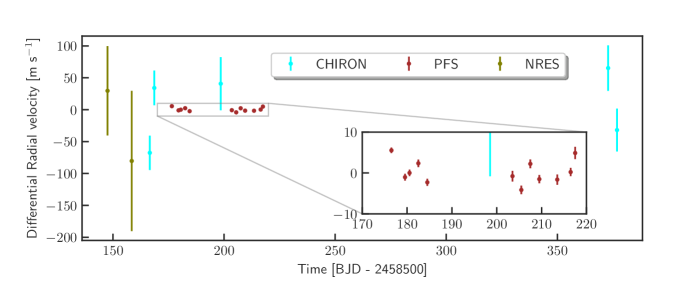
Figure 4: Differential radial velocities of HD 108236 measured as part of the SG2 and SG4 subgroups, modeled using a sinusoidal (i.e., non-eccentric) model. NRES, CHIRON, and PFS data are shown with the colors olive, cyan, and brown, respectively. The data from each instrument are shown after subtracting the weighted mean.

The currently available radial velocity data cannot rule out stellar companions at arbitrary orbital periods, eccentricities and inclinations. Therefore, a remaining false positive hypothesis would be a hierarchical system containing planets transiting the primary or the secondary. However, the transiting planets would also have to be giants in this case, in order to compensate for the dilution from the companion star. If more than one such giant planets orbited the companion star, the system would be dynamically unstable. The multiplicity of the transiting objects in the system makes this false positive hypothesis unlikely. Furthermore, as has been shown in Latham et al. (2011); Lissauer et al. (2012); Guerrero et al. (submitted), it is much less likely for a planet candidate to be a false positive in a multiplanetary system than in a system with a single planet. We therefore discarded this false positive hypothesis based on the observation of four independent TCEs.

3.6 High-resolution speckle imaging

In order to rule out aligned foreground or background stars at close separations, high-resolution images are needed. To obtain high-resolution images in the presence of atmospheric scintillation, we used the speckle imaging technique by taking short exposures of the bright target to factor out the effect of atmospheric turbulence. For this purpose, we used the resources of the SG3 subgroup of TFOP and obtained high-resolution speckle images of HD 108236 with SOAR/HRCam and Gemini/Zorro.

3.6.1 SOAR/HRCAM

Diffraction-limited resolution was obtained via speckle interferometry by using the High-Resolution Camera (HRCam) (Tokovinin et al., 2010; Ziegler et al., 2020) at the 4.1-meter SOAR telescope by processing short-exposure images taken with high magnification on UT 7 January 2020. The autocorrelation function and the resulting sensitivity curve are presented in the left panel of Figure 5. A contrast of 5 magnitudes is achieved at a separation of 0$\farcs$2.

3.6.2 Gemini/Zorro

We obtained speckle interferometric images of HD 108236 on UT 14 January 2020 and UT 12 March 2020 using the Zorro instrument on the 8-meter Gemini South telescope at the summit of Cerro Pachon in Chile. Zorro simultaneously observes in two bands, i.e., $832\pm 40$ nm and $562\pm 54$ nm, obtaining diffraction limited images with inner working angles of 0.017″and 0.026″, respectively. Both data sets consisted of 3 minutes of total integration time taken as sets of a thousand 0.06-second images. Each night’s data were combined and subjected to Fourier analysis leading to the production of final data products including speckle reconstructed imagery. The right panel of Figure 5 shows the 5-sigma contrast curves in both filters for data collected on UT 12 March 2020 and includes an inset showing the 832 nm reconstructed image. The speckle imaging results in both observations agree, revealing HD 108236 to be a single star to contrast limits of 5.5 to 8 magnitudes within a sky-projected separation between 1.3 and 75 Astronomical Unit (AU).

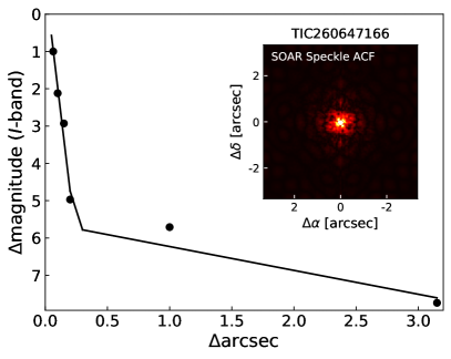
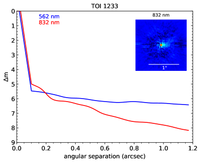
Figure 5: The 5-$\sigma$ sensitivity curve of speckle imaging by SOAR/HRCam (left) and Gemini/Zorro (right). The inset on the left shows the two-dimensional autocorrelation function, whereas the inset on the right is a reconstructed image of the field. The data rule out bright neighbors and companions to HD 108236, which would be fully spatially-blended in the TESS images.

These high-resolution images rule out wide stellar binaries that would not be spatially-resolved in ground-based, seeing-limited photometry with a PSF of $\sim$ 1″. In addition, using the Dartmouth isochrone model (Dotter et al., 2008), they imply that a bound companion to HD 108236 would have to be less massive than 0.10-0.15 M_⊙, depending on the age of the system.

Table 6: High-resolution imaging data collected on HD 108236.

Telescope	SOAR
Instrument	HRCam
Filter	$879\pm 289$ nm
Image Type	Speckle
Pixel Scale [as]	0.01575
Estimated PSF [as]	0.06364
Telescope	Gemini
Instrument	Zorro
Filter	$832\pm 40$ nm, $562\pm 54$ nm
Image Type	Speckle
Pixel Scale [as]	0.01
Estimated PSF [as]	0.02

3.7 Seeing-limited (ground-based) transit photometry

After ruling out binaries and chance alignments for the target, we then proceeded with ruling out the possibility that the transits detected by TESS could be on nearby stars. HD 108236 is the brightest source within a few arcminutes in its vicinity. Given the depth of the transits observed by TESS ($0.302\pm 0.031$ ppt, $0.517_{-0.040}^{+0.036}$ ppt, $0.889\pm 0.053$ ppt, and $1.175\pm 0.069$ ppt), the transit depth would have to be deeper by a certain amount as given by Equations 1 and 2 if the transit was not on HD 108236, but rather on a fainter nearby target. In order to rule out the hypothesis that any of the transits could be on a nearby target, we collected seeing-limited (i.e., with a PSF full-width at half maximum of $\sim$ 1 as) photometric time-series data during a predicted transit for each planet candidate (i.e., TOIs 1233.01, 1233.02, 1233.03 and 1233.04) using the resources of the SG1 subgroup of TFOP including the LCOGT and MEarth telescopes. Table 7 lists these observations. As will be discussed in Section 3.7.4, one of these observations (UT 17 March 2020) resulted in a tentative detection of a transit on target.

3.7.1 LCOGT

We used LCOGT (Brown et al., 2013) of 1-meter class telescopes to obtain ground-based transit light curves of all four planet candidates of HD 108236. We used the TESS Transit Finder, which is a customized version of the Tapir software package (Jensen, 2013), to schedule our transit observations. Specifically, observations were taken from the CTIO and South African Astronomical Observatory (SAAO) LCOGT locations. Both telescopes are equipped with a $4096\times 4096$ pixel Sinistro camera whose pixel scale is 0.389″, resulting in a $26^{\prime}\times 26^{\prime}$ field-of-view. We achieved a typical PSF FWHM of 2.3″, which is about 30 times smaller than the TESS PSF. Each image sequence was calibrated using the standard BANZAI pipeline (McCully et al., 2018) while the differential light curves of HD 108236 and its neighbouring sources were derived using the AstroImageJ software package (Collins et al., 2017).

Table 7 summarizes our eight successful transit observations from LCOGT taken between UT 11 January 2020 and UT 17 March 2020. Explicitly, we collected data during two, three, two, and one transits of TOIs 1233.01, 1233.02, 1233.03, and 1233.04, respectively. All light curves were obtained with either 20 or 60-second exposures in either the $y$ or $z_{\rm s}$ bands to optimize photometric precision. Photometric apertures were selected by the individual SG1 observer based on the FWHM of the target’s PSF in order to maximize the photometric precision. In each light curve we tested all bright neighbouring sources within $2.5^{\prime}$ of HD 108236. Then we either tentatively detected the expected transit event on the target (i.e., on UT 17 March 2020 with LCOGT-CTIO) or were able to rule out transit-like events on all nearby targets down to the faintest neighbor magnitude contrasts reported in Table 7 (i.e., during all other observations). For each planet candidate, all known Gaia DR2 stars within 2.5 arcminutes of HD 108236 that are bright enough to cause the TESS detection were ruled out as possible sources of the TESS detections.

3.7.2 MEarth-South

MEarth-South employs an array of eight f/9 40-cm Ritchey–Chrétien telescopes on German equatorial mounts (Irwin et al., 2015). During the data acquisition for this work, only seven of the telescopes were operational. Data were obtained on three nights: UT 3 March 2020 (egress of TOI 1233.01), UT 11 March 2020 (full transits of TOI 1233.02 and TOI 1233.03) and UT 17 March 2020 (full transit of TOI 1233.01). Figure 6 shows the in-focus and defocused fields of the MEarth-South observation on UT 17 March 2020.

All observations were conducted using the same observational strategy. Exposure times were 35 seconds with six telescopes defocused to half flux diameter of 12 pixels to provide photometry of the target star, and one telescope observing in-focus with the target star saturated to provide photometry of any nearby or faint contaminating sources not resolved by the defocused time series. Observations were gathered continuously starting when the target rose above 3 air masses (first observation) or evening twilight (other observations) until morning twilight. Telescope 7 used in the defocused set had a stuck shutter resulting in smearing of the images during readout, but this did not appear to affect the light curves. The defocused observations were performed with a pixel scale of 0.84″. A photometric aperture with a radius of 17 pixels was used to extract the photometric time-series. Data were reduced following standard procedures for MEarth photometry (Irwin et al., 2007).

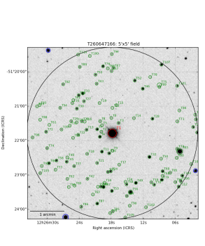
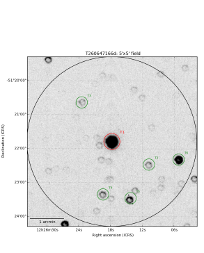
Figure 6: A photometric image of the field in the vicinity of HD 108236 as observed by MEarth-South on UT 17 March 2020. The left panel shows the image in focus as collected by one of the MEarth-South telescopes, where HD 108236 is saturated due to its brightness. The right panel shows the defocused image as observed by the other six MEarth-South telescopes. In these images the PSF is broader, unsaturating HD 108236 and allowing precision photometry on the target.

3.7.3 Ruling out nearby eclipses and transits

During the predicted transit of each planet candidate (i.e., TOI 1233.01, TOI 1233.02, TOI 1233.03, and TOI 1233.04), light curves of all nearby stars were extracted and checked for any transits with a depth that could cause the relevant transits in the TESS light curves. No such transit was observed for any of the planet candidates. These data ruled out the hypotheses that any of the transits detected by TESS could be off-target by ensuring that no nearby star transited at the predicted transit time.

Upon collecting the above time-series and ruling out transits on nearby targets, we finally concluded that the planetary nature of the transiting objects were validated. Thus, in the remainder of this paper, we will refer to these transiting planets as HD 108236 b, HD 108236 c, HD 108236 d, and HD 108236 e, (or simply as planet b, c, d, and e) ordered with respect to increasing distance from the host star, HD 108236. Note that these four planets correspond to TOIs 1233.04, 1233.03, 1233.01, and 1233.02, respectively.

3.7.4 Ground-based detection of a transit

A transit of planet d was tentatively detected on UT 17 March 2020 at a 1-meter LCOGT-CTIO telescope. The photometric time-series data had a relatively short pre-transit baseline. Therefore, we excluded these observations from the global orbital model in Section 3.9, in order to avoid biasing the fit. However, we fitted the LCOGT-CTIO data separately and inferred a transit duration of $3.8\pm 0.2$ hours and a transit depth of $1.1\pm 0.2$ ppt, which are consistent with those inferred from the TESS data. The inferred mid-transit time was $2458571.3365\pm 0.0035$ BJD, indicating a transit arrival 14 minutes late compared to the linear ephemeris model based on the TESS data. The associated light curve is shown in Figure 7.

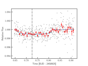
Figure 7: Detrended follow-up light curve of HD 108236 during the transit of planet d as measured by LCOGT-CTIO, where the transit was tentatively confirmed to be on-target. The transit arrived 14 minutes late, which is expected given the ephemeris uncertainty of $\sim$ 1 hour. The vertical line shows the mid-transit time of the transit that was expected based on the linear ephemeris inferred from the TESS data. The gray and red points denote the raw and binned data and the blue line is the posterior median transit model.

Table 7: Ground-based photometric time-series observations made on HD 108236 during the predicted transits based on the TESS TCEs.

Date	Telescope	Camera	Filter	Pixel	PSF	AR	Transit	FN	Duration	Obs
[UT]				[as]	[as]	[Pixel]		[Mag]	[minutes]
TOI 1233.01
2020-03-02	LCOGT-SAAO-1m	Sinistro	zs	0.39	2.0	20	Full	8.1	341	376
2020-03-03	MEarth-South	Apogee	RG715	0.84	2.1	8.5	Egress	9.9	587	577
2020-03-03	MEarth-Southx6	Apogee	RG715	0.84	8.0	17	Egress	5.5	588	3621
2020-03-17	LCOGT-CTIO-1m	Sinistro	zs	0.39	2.5	15	Full	n/c	384	434
2020-03-17	MEarth-South	Apogee	RG715	0.84	2.1	8.5	Full	9.9	620	608
2020-03-17	MEarth-Southx6	Apogee	RG715	0.84	8.1	17	Full	5.5	620	3819
TOI 1233.02
2020-01-11	LCOGT-CTIO-1m	Sinistro	y	0.39	1.8	10	Ingress	8.0	223	148
2020-01-31	LCOGT-SAAO-1m	Sinistro	y	0.39	2.6	15	Egress	8.3	309	174
2020-03-11	MEarth-Southx6	Apogee	RG715	0.84	7.9	17	Full	5.5	610	3759
2020-03-11	MEarth-South	Apogee	RG715	0.84	1.9	8.5	Full	11	609	584
2020-03-11	LCOGT-CTIO-1m	Sinistro	zs	0.39	2.0	11	Full	7.7	455	507
TOI 1233.03
2020-02-02	LCOGT-SAAO-1m	Sinistro	zs	0.39	3.1	10	Full	8.6	296	192
2020-03-11	LCOGT-CTIO-1m	Sinistro	zs	0.39	1.8	15	Full	n/c	452	507
TOI 1233.04
2020-01-11	LCOGT-SAAO-1m	Sinistro	zs	0.39	3.0	6	Full	9.2	205	143

FN stands for the faintest neighbor and the column values indicate the magnitude difference of the faintest neighbor checked for an NEB. In this column, (n/c) indicates ”not checked” since transit-like events on nearby targets in the field at the same ephemeris were ruled out previously.

3.8 Archival ground-based photometry

HD 108236 has also been observed by the Wide Angle Search for Planets South (WASP-South) survey (Pollacco et al., 2006) in SAAO, South Africa. WASP-South, an array of 8 wide-field cameras, was the Southern station of the WASP transit-search project (Pollacco et al., 2006). It observed the field of HD 108236 in 2011 and 2012, when equipped with 200-mm, f/1.8 lenses, and then again in 2013 and 2014, equipped with 85-mm, f/1.2 lenses. It observed on each clear night, over a span of 140 nights in each year, with a typical 10-minute cadence, and accumulated about 58,000 photometric measurements on HD 108236. We searched the data for any rotational modulation using the methods from Maxted et al. (2011). We found no significant periodicity between 1 and 80 days, with a 95% confidence upper limit on the amplitude of 1 mmag. We did not detect any transits in the WASP data, consistent with the expected small transit depths of $0.302\pm 0.031$, $0.517_{-0.040}^{+0.036}$, $0.889\pm 0.053$, and $1.175\pm 0.069$ ppt. Planet e had the deepest expected transit, however its relatively long period likely precluded any detection. The shallow transits of the inner planets also made them undetectable. To determine which region of the parameter space of transiting planets can be ruled out with the WASP data set, we performed injection-recovery tests using allesfitter, which will be introduced in Section 3.9. We injected planets over a grid of periods of 10.1, 15.1, …, 140.1 days and radii of 8, 8.5, …, 22 R_⊕. For each planet, we tried to recover the injected signal using Transit Least Squares (TLS, Hippke & Heller, 2019). We find that $\sim$50% of transiting planets with radii 1.3–2 R_J and periods less than 100 days could have been found in the WASP data. The recovery rate drops to $\sim$20% for planets with radii $\sim$1 R_J and periods less than 100 days. In contrast, planets much smaller than Jupiter or those on periods longer than 100 days would remain undetected in the WASP data.

3.9 Transit model

Following the vetting of the planet candidates, we modeled the TESS PDC light curve to infer the physical properties of the orbiting planets. In order to model the photometric time-series data, we used allesfitter (Günther & Daylan, 2019, 2020). The parameters $\theta$ of our forward model $M$ are presented in Table 8. We assumed a transit model with a linear ephemeris. We assumed a generic, eccentric orbit. For limb darkening, we used a transformed basis $q_{1}$ and $q_{2}$ of the linear $u_{1}$ and quadratic $u_{2}$ coefficients as (Kipping, 2013)

$$q_{1}=(u_{1}+u_{2})^{2},$$ (3)

$$q_{2}=0.5\dfrac{u_{1}}{u_{1}+u_{2}}.$$ (4)

We modeled this red noise along with any other stellar variability in the data using a Gaussian Process (GP) with a Matérn 3/2 kernel as implemented by celerite (Foreman-Mackey et al., 2017).

Table 8: Parameters of the transit forward-model.

Parameter	Explanation	Prior
$q_{1;\mathrm{TESS}}$	First limb darkening parameter 1	uniform
$q_{2;\mathrm{TESS}}$	Second limb darkening parameter 2	uniform
$\log{\sigma_{\mathrm{TESS}}}$	Logarithm of the scaling factor for relative flux uncertainties	uniform
$\log{\sigma_{\rm GP;\mathrm{TESS}}}$	Amplitude of the Gaussian process Matérn 3/2 kernel	uniform
$\log{\rho_{\rm GP;\mathrm{TESS}}}$	Time scale of the Gaussian process Matérn 3/2 kernel	uniform
$D_{\mathrm{0;TESS}}$	Dilution of the transit depth due to blended light from neighbors	fixed
$R_{\rm n}/R_{\star}$	Ratio of planet $n$, $R_{\rm n}$, to the radius of the host star, $R_{\star}$	uniform
$(R_{\star}+R_{\rm n})/a_{\rm n}$	Sum of the stellar radius $R_{\star}$ and planetary radius $R_{\rm n}$	uniform
$\cos{i_{\rm n}}$	cosine of the orbital inclination, $i$	uniform
$T_{0;\rm n}$	Mid-transit time about which the linear ephemeris model pivots, i.e., epoc, in $\mathrm{BJD}$	uniform
$P_{\rm n}$	Orbital period of planet $n$ in days	uniform
$\sqrt{e_{\rm n}}$ $\cos{\omega_{\rm d}}$	Square root of the eccentricity times the cosine of the argument of periastron	uniform
$\sqrt{e_{\rm n}}$ $\sin{\omega_{\rm d}}$	Square root of the eccentricity times the sine of the argument of periastron	uniform

When modeling the TESS data, we use the PDC light curve data product from the SPOC pipeline. We provide the posterior in Table 11 for nuisance parameters, Table 13 for the parameters of planets b and c, and Table 12 for the parameters of planets d and e. We then provide the derived posterior in Table 14 for planets b and c and Table 15 for planets d and e. Although our nominal results come from allesfitter, we have also repeated the analysis using EXOFASTv2 (Eastman et al., 2019) as a cross check in order to confirm consistency. EXOFASTv2 has a dynamical prior that avoids orbit crossings and ensures dynamical stability of the analyzed system. A notable result from this analysis were additional constraints on the eccentricities of the planets enabled by the Hill stability prior. The inferred eccentricities were smaller than 0.287, 0.197, 0.164, and 0.149 at a confidence level of 2$\sigma$ for planets b, c, d, and e, respectively.

We show in Figure 8 the light curve of each planet folded onto its orbital period and centered at the phase of the primary transit, after masking out the transits of the other planets. Because the orbital period of planet d is close to the orbital period of TESS around the Earth ($\sim$ 13.7 days), a large gap is formed in its phase curve. Figure 9 then shows the individual phase curves, along with the posterior-median transit model shown with the blue lines.

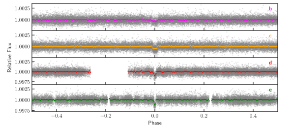
Figure 8: Detrended PDC light curve folded at the posterior median period of each planet after masking out the transits of other planets. Close-in views of the transits are also given in Figure 9.

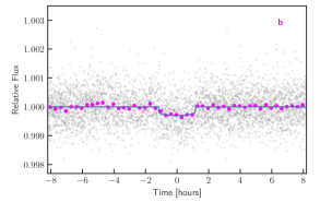
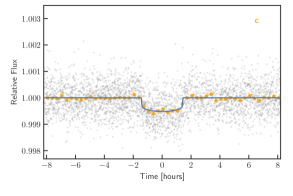
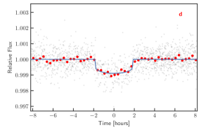
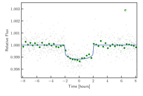
Figure 9: Phase curves of the four discovered planets. Blue lines indicate the posterior median of the transit model fitted to the data.

4 The HD 108236 system

In this section, we review the main properties of the planets discovered to be transiting HD 108236. The HD 108236 system is depicted in Figure 10. The transiting planets b, c, d, and e orbit the host star on orbits with semi-major axes of $0.0469\pm 0.0017$ AU, $0.0651\pm 0.0024$, $0.1131\pm 0.0040$ AU, and $0.1400\pm 0.0052$ AU, respectively. Compared to our Solar System, the discovered planets orbit rather closer to their host star, HD 108236, forming a closely-packed, compact multiplanetary system.

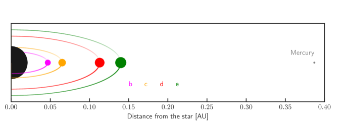
Figure 10: Inclined view of the HD 108236 system. The horizontal axis denotes the distance from the host star, HD 108236, which is shown on the left with a black circle. The four planets HD 108236 b, HD 108236 c, HD 108236 d and HD 108236 e are shown with magenta, orange, red and green, respectively. Shown on the far right with gray is Mercury as it would look if it orbited HD 108236 at its current orbital period. The radii of the planets and the star are scaled up by a factor of 50 and 5, respectively. The elliptical appearance of the orbits are due to the viewing angle and do not make any implication about the orbital eccentricities.

HD 108236 b is a hot super-Earth with a radius of $1.586\pm 0.098$ $R_{\oplus}$. Being the innermost discovered planet of the system, it has a period of $3.79523_{-0.00044}^{+0.00047}$ days, making it the hottest known planet in the system with an estimated equilibrium temperature of $1099_{-18}^{+19}$ K. The other three known planets in the system are HD 108236 c, HD 108236 d, and HD 108236 e. These are sub-Neptunes with radii $2.068_{-0.091}^{+0.10}$ $R_{\oplus}$, $2.72\pm 0.11$ $R_{\oplus}$, and $3.12_{-0.12}^{+0.13}$ $R_{\oplus}$ and periods $6.20370_{-0.00052}^{+0.00064}$ days, $14.17555_{-0.0011}^{+0.00099}$ days, and $19.5917_{-0.0020}^{+0.0022}$ days, respectively. Their equilibrium temperatures are $932_{-16}^{+17}$ K, $708_{-12}^{+13}$ K, and $636_{-11}^{+12}$ K, respectively, under the assumption of an albedo of 0.3.

Figure 11 compares the inferred radii of the validated planets b, c, d, and e to the occurrence rate of planets as a function of planetary radius. Planet b is especially interesting for studies of photoevaporation, since its radius of $1.586\pm 0.098$ $R_{\oplus}$ falls within a relatively uncommon radius range known as the radius valley (Fulton et al., 2017). The radius valley is thought to be depleted due to photoevaporation caused by the stellar wind of the host star (Owen & Wu, 2017). However, the location of this radius valley has been shown to be a function of insolation flux (Van Eylen et al., 2018). Larger rocky planets can exist in more extremely irradiated environments. With an equilibrium temperature of $1099_{-18}^{+19}$ K, planet b is consistent with being part of the population of small, rocky planets just below the radius valley. In contrast, the planets c, d, and e are typical sub-Neptunes.

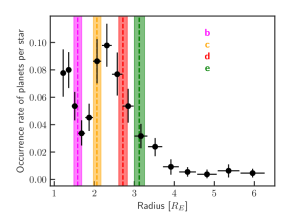
Figure 11: The radii of the planets transiting HD 108236 compared to the completeness-corrected occurrence rate of planets with orbital periods less than 100 days (Fulton et al., 2017). The posterior median and 68% credible interval of radii of the planets hosted by HD 108236 are highlighted with vertical lines and bands, respectively. Planet b falls within the radius valley (Fulton et al., 2017).

4.1 Bright host

HD 108236 is one of the brightest stars that host four or more planets. As shown in the top row of Figure 12, it is the third (behind Kepler 444 (Campante et al., 2015) and HIP 41378 (Vanderburg et al., 2016)) and the fourth brightest star (behind Kepler 444, HIP 41378, and Kepler 37 (Barclay et al., 2013)) in the V and J bands, respectively, that is known to host at least four planets. However, out of these, only Kepler 37 is a Sun-like star, making HD 108236 the brightest Sun-like star in the visual band to harbor at least four transiting planets. This property of HD 108236 makes it an interesting and accessible target from an observational point-of-view regarding future mass measurements, photometric follow-up and atmospheric characterization of its transiting planets.

The bottom row of Figure 12 also shows the radial velocity semi-amplitude (at fixed planet mass and orbital period) divided by the square root of the host star brightness in the V and J bands, respectively, which are denoted by $K^{\prime}_{V}$ and $K^{\prime}_{J}$. The x-axes are normalized so that the top target has the value of 1. Being a Sun-like star, HD 108236 falls to the 7^th rank, when the comparison is made in the J band, since low-mass stars generate a larger radial velocity signal for a given companion.

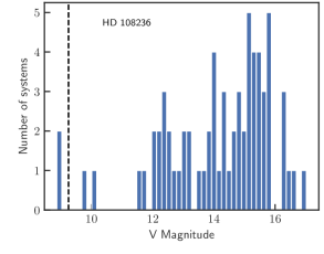
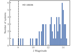
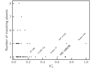
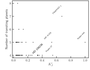
Figure 12: Comparison of HD 108236 to other systems with at least four transiting exoplanets. Top: histograms of the V (left) and J band (right) magnitudes of systems that were previously known to host at least four transiting exoplanets. The magnitudes of HD 108236 are highlighted with dashed vertical black lines. Bottom: the radial velocity semi-amplitude (at fixed planet mass and orbital period) divided by the square root of the host star brightness in the V (left) and J (right) bands, denoted by $K^{\prime}_{V}$ and $K^{\prime}_{J}$. The x-axes are normalized such that the largest value is 1. We highlight the top 5 previously known systems retrieved from the NASA Exoplanet Archive. In the lower panel, the exoplanet labels are placed to the upper left of the corresponding points. HD 108236 is highlighted with crosses.

4.2 Mass measurement potential of the transiting planets

The expected radial velocity semi-amplitudes of the four validated planets based on the predicted masses are in the range of 1.3–2.4 m s^-1. Given the brightness of the host star, this implies that the system has good potential for mass measurements in the near future. There are ongoing efforts to measure the masses of all validated transiting planets hosted by HD 108236.

Given the current absence of mass measurements of the planets, we use the probabilistic model of Chen & Kipping (2017) in order to predict the masses of the validated planets. This model takes into account the measurement, sampling and intrinsic scatter of known planets in the mass-radius plane. As a result, the large uncertainties of the resulting mass predictions are dominated by this intrinsic system-to-system scatter and not by the posterior radius uncertainties of the planets validated in this work.

The masses of planets b, c, d, and e are predicted as $4\pm 2$, $5\pm 3$, $8\pm 5$, and $10\pm 6$ M_⊕, respectively. Hence, planet b is likely a dense, rocky planet, whereas planets c, d, and e are sub-Neptunes with a hydrogen and helium envelope whose radius increases going from planet c to e. Atmospheric escape of volatiles is likely to be strongest for the innermost planet b, and should decrease towards the outermost planet e.

4.3 Atmospheric characterization potential

Once the radius, mass and, hence, the bulk composition of a planet are determined, the next step in its characterization is the determination of its atmospheric properties. The available data on HD 108236 do not yet allow the atmospheric characterization of its planets. However, sub-Neptunes orbiting HD 108236 are favorable targets for near-future atmospheric characterization as we discuss below.

Given the expected launch of the James Webb Space Telescope (JWST), the Transmission Spectrum Metric (TSM) (Kempton et al., 2018),

$$\text{TSM}\propto\dfrac{R^{3}_{\rm p}T_{\rm eq}}{M_{\rm p}R_{\star}^{2}},$$ (5)

ranks the relative SNR of different planets assuming observations made with the Near Infrared Imager and Slitless Spectrograph (NIRISS) (Maszkiewicz, 2017) of JWST, assuming a cloud-free, hydrogen-dominated atmosphere.

The largest uncertainty in predicting the TSMs of the planets orbiting HD 108236 arises from the current unavailability of their mass measurements. We use the predicted masses of planet b, c, d, and e in Equation 5 to obtain preliminary estimates of their TSMs. Based on the brightness of the host star, it is expected that the masses of all validated planets will be measured to better than 40%. Therefore, comparing the TSMs of the validated planets to those of all known sub-Neptunes retrieved from the NASA Exoplanet Archive Planetary Systems Composite Data with mass measurement uncertainties better than 5$\sigma$, we find that the sub-Neptunes HD 108236 c, HD 108236 d, and HD 108236 e fall among the top 20. The super-Earth (planet b) is not included in this TSM ranking, because it is not expected to have a hydrogen-dominated atmosphere. We once again emphasize that these rankings are based on the predicted masses and the actual rankings will depend on the mass measurements of the planets.

The logarithms of the relative TSMs of the planets are plotted against their radii in Figure 13, along with those of the known exoplanets (black points) retrieved from the NASA Exoplanet Archive, where the overall normalizations of the TSMs is arbitrary. We only show those known planets that have a measured mass with an uncertainty better than 40%. The three sub-Neptunes of the HD 108236 system are found to be favorable targets for comparative characterization of sub-Neptune atmospheres.

It is worth noting that the TSM ranking of the HD 108236 sub-Neptunes improves with decreasing equilibrium temperature, despite the fact that lowering the temperature acts to reduce the pressure scale height.

As can be seen in Equation 5, the TSM is proportional to the third power of $R_{p}$, while inversely proportional to $M_{p}$. Although it also scales with $M_{p}$, the $R_{p}$ dependence of $M_{p}$ is weaker than $R_{p}^{3}$. Therefore, the TSM is more sensitive to an increase in planetary radius than a drop in equilibrium temperature. In the HD 108236 system, the radii of the planets c, d, and e increase with decreasing equilibrium temperature. As a result, the predicted TSM increases from planet c to e.

Furthermore, although HD 108236 is a relatively bright target, its brightness is below the limiting magnitude of NIRISS/JWST (J magnitude of $\sim$ 7) (Beichman et al., 2014), making it an appealing transmission spectroscopy target for the instrument.

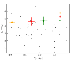
Figure 13: The logarithm of TSM vs. radius distribution of the sub-Neptunes orbiting HD 108236 and known transiting planets with mass measurements better than 5$\sigma$ as retrieved from the NASA Exoplanet Archive. Planets c, d, and e of HD 108236 are among the top 20 known sub-Neptunes when ranked with respect to their TSMs.

We also note that planets orbiting HD 108236 span a broad range of radius and equilibrium temperature. Figure 14 shows the distribution of radii and equilibrium temperatures of known planets retrieved from the NASA Exoplanet Archive and those of the planets orbiting HD 108236. The wide range of radii and equilibrium temperatures manifested by the planets allows controlled experiments of how stellar insolation affects the photoevaporation of the volatile envelopes of the orbiting planets by controlling for the stellar type and evolution history(Owen & Campos Estrada, 2020).

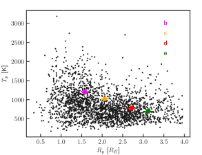
Figure 14: The equilibrium temperatures and radii of known planets retrieved from the NASA Exoplanet Archive, shown with black points. Planets orbiting HD 108236 are highlighted, which span a broad and representative range of radius and equilibrium temperature.

4.4 Dynamics

In a multiplanetary system, the displacement from a mean motion resonance (MMR)

$$\Delta=\frac{P^{\prime}}{P}\frac{j-k}{j}-1,$$ (6)

of adjacent planet pairs characterizes the proximity of the pair to a MMR, where $P^{\prime}$ and $P$ are the orbital periods of the outer and inner planets, $j$ is the nearest integer to the orbital period ratio, and $k$ is the order of the nearest MMR. Proximity to an MMR results in TTVs with a coherence time scale (i.e., super-period) of $P_{\rm ttv}$ such that

$$\frac{1}{P_{\rm ttv}}=\left|\frac{j-k}{P}-\frac{j}{P^{\prime}}\right|.$$ (7)

The HD 108236 system consists of closely packed planets. However, no pair of the validated planets is on an MMR. The proximities and super-periods of the known adjacent pairs in the HD 108236 system are shown in Table 9.

Pair	$P^{\prime}/P$	j:j-k	$\Delta$	Pttv [day]
b,c	1.63473	5:3	-0.01916	64.75626
c,d	2.28506	9:4	0.01558	101.08835
d,e	1.37870	4:3	0.03403	143.61021

Table 9: Proximities to MMRs of adjacent planet pairs in the HD 108236 system. The second and third columns list the orbit period ratios and nearest MMR, while the fourth and fifth columns estimate the proximity to resonance and the coherence period respectively. The outer pair is near a first order resonance where we noted the estimated TTV amplitude in the last two columns, as described in the text.

For the first order interaction between a pair, where $k=1$, the amplitude of the TTVs, $V$ and $V^{\prime}$, can be estimated using the analytical solution (Lithwick et al., 2012)

$$V =P\frac{\mu^{\prime}}{\pi j^{2/3}(j-1)^{1/3}\Delta}\left(-f-\frac{3}{2}\frac{Z_{\rm free}^{*}}{\Delta}\right),$$ (8)

$$V^{\prime} =P^{\prime}\frac{\mu}{\pi j\Delta}\left(-g+\frac{3}{2}\frac{Z_{\rm free}^{*}}{\Delta}\right),$$ (9)

where $f$ and $g$ are coefficients, $\mu$ and $\mu^{\prime}$ are the masses of the planets normalized by that of the host star, and $Z_{\rm free}^{*}$ is the conjugate of the complex sum of eccentricity vectors.

No planet pairs in the HD 108236 system are in or near a strong MMR, precluding the generation of large resonant TTVs. However, non-resonant (chopping) TTVs with small amplitudes induced by synodic interactions, are possible. Assuming circular orbits and using the predicted masses yield a TTV of $\sim$ 5 minutes for both planet d and e. We also confirmed this analytical prediction using an N-body dynamical simulation (Lissauer et al., 2011) of HD 108236 with a length of 5000 days. We note that the planets could have higher TTVs when the circular orbit assumption is relaxed. Hence, with sufficient transit timing precision, planets d and e are likely to be amenable to mass measurements via TTV observations enabled by long-term transit photometry follow-up (Deck & Agol, 2015).

Potential 3-body resonances due to a hypothetical planet x

The orbital gaps between planet b and c and between planet c and d are large enough for low mass planets to exist on stable orbits, as is common among multiplanetary systems discovered by the Kepler telescope. There are many adjacent pairs in the Kepler data set close to the 3:2 MMR, which invokes the possibility of a missing planet in the apparent 9:4 near resonant gap between the middle pair of HD 108236. While the parameter space for such missing planets is fairly large, we note that resonant chains of 3 bodies, as is present in systems like TRAPPIST-1 (Gillon et al., 2017) and Kepler-80 (Xie, 2013), could be present in HD 108236 due to yet-undetected planets. This undetected planet x could either have a period of $P_{\rm x}$ = 9.364 days, which would satisfy

$$0\approx 2n_{\rm c}-5n_{\rm x}+3n_{\rm d},$$ (10)

where $n_{\rm x}$ is the orbital frequency of the hypothetical planet, or a period of P_x = 9.150 days, which would satisfy

$$0\approx n_{\rm x}-3n_{\rm d}+2n_{\rm e}.$$ (11)

The resulting 3:2 resonance between this hypothetical planet x and planet d would result in additional TTVs.

To search for evidence of such an additional planet in the TESS data, we used allesfitter’s interface to remove the remnant stellar variability from the PDC light curve using a cubic spline and recursive sigma clipping via wotan (Hippke et al., 2019). Then, we ran a TLS search (Hippke & Heller, 2019) on this flattened light curve. We recovered all four transiting planets b,c, d, and e. We also detected several additional periodic transit-like signals above an SNR threshold of 5. The most statistically significant of these detections has an epoch of 2458570.6781 BJD, period of $10.9113$ days, transit depth of $0.23$ ppt, SNR of 8.0, signal detection efficiency (SDE) of 6.9, and false alarm probability of 0.01. We therefore present this as a tentative fifth planet candidate in the HD 108236 system. However, given the large false positive probability and its dependence on the detrending method, we concluded that instrumental origin cannot be ruled out for this planet candidate. In particular, the stellar density consistent with the transits of this candidate is $0.4\pm 0.3$ g cm^-3, which is inconsistent with the stellar density ($1.9$ g cm^-3) inferred in Section 2. This implies that the candidate is likely due to systematics. Given the larger false positive probabilities of the other TLS detections (i.e., larger than 0.01), we discarded them as likely due to systematics in the TESS data.

TTV analysis of TESS transits

In order to infer the TTVs consistent with the TESS data, we performed a light curve analysis independent of that discussed in Section 3.9 using exoplanet (Foreman-Mackey et al., 2020) by relaxing the assumption of a linear ephemeris. The resulting TTVs are shown in Figure 15. Table 10 also tabulates the mid-transit times of the transits detected in the TESS data. We did not detect any significant TTVs given the temporal baseline and timing precision of the transits observed by TESS. Nevertheless, using these TTVs, we were able to constrain the mass of planet e to be lower than 31 M_⊕ at 2$\sigma$ via the dynamical simulation, which is consistent with the mass predicted via Chen & Kipping (2017).

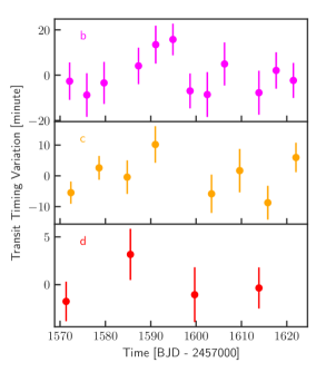
Figure 15: The measured TTVs of the discovered planets in the HD 108236 system. The measured mid-transit times are consistent with a linear ephemeris model. No TTV for planet e was measured, since only two transits were observed.

Table 10: Measured mid-transit times of planets b, c, and d in the TESS data. All times are provided in BJD after subtracting 2,457,000.

Mid-transit time [BJD - 2,457,000]	1$\sigma$ uncertainty [days]
Planet b
1572.107037	0.006751046
1575.898507	0.007962894
1579.697924	0.007157883
1587.294548	0.00576889
1591.096759	0.005991691
1594.894048	0.00481626
1598.673998	0.005489018
1602.468591	0.007256515
1606.273666	0.007104524
1613.856271	0.007697341
1617.658793	0.006202734
1621.451437	0.00614042
Planet c
1572.391729	0.002815299
1578.601024	0.002967442
1584.802628	0.004321249
1591.013683	0.004541912
1603.409944	0.004748817
1609.618876	0.005754455
1615.815326	0.004564704
1622.029226	0.003369172
Planet d
1571.335310	0.00213619
1585.514907	0.002414469
1599.688154	0.002331228
1613.864821	0.002721803

Stability

To further test the dynamical integrity of the system, we conducted N-body integrations using the Mercury Integrator Package (Chambers, 1999). Our method is similar to that adopted by (Kane, 2015, 2019) in the study of compact planetary systems discovered by Kepler. The innermost planet of our system has an orbital period of $\sim$3.8 days. To ensure perturbative accuracy, we therefore used a conservative time step for the simulations of 0.1 days, which is $\sim 1/40$ of the period of the innermost planet. We ran the simulation for $10^{7}$ years, equivalent to $\sim 10^{9}$ orbits of the innermost planet. For the masses of the planets b, c, d, and e, we assumed fiducial values of 3.5, 4.7, 7.2, and 11.1 M_⊕. The results of the simulation are represented in Figure 16 by showing the histogram of the eccentricities of the four planets for the entire simulation. The results show that the system is dynamically stable, even considering the non-zero eccentricities for such a compact system. However, there is significant transfer of angular momentum that occurs between the planets with time. The two innermost planets have eccentricities that oscillate between 0 and $\sim 0.13$, which can result in substantial changes in the climate of the atmospheres (Kane & Torres, 2017; Way & Georgakarakos, 2017), known as Milankovitch cycles (Spiegel et al., 2010). The two outermost planets, d and e, remain near their starting eccentricities and so are largely unperturbed through the orbital evolution.

Figure 16: Histograms of the eccentricities inferred from the dynamical stability simulation. The system retains orbital integrity throughout the $10^{7}$ year simulation time.

5 Discussion and Conclusion

Systems with multiple planets provide a test bed for models of planet formation, evolution and orbital migration. Roughly one-third of the planetary systems discovered by the Kepler telescope are multiplanetary (Borucki et al., 2011). The inferred valley in the radius distribution of known, small planets (Fulton et al., 2017) is possibly due to the photoevaporation of volatile gases on close-in planets or core-powered mass loss (Ginzburg et al., 2018). These processes can leave behind a rocky core and a small (less than 2 $R_{\oplus}$) radius, while the unaffected population constitute gas giants with radii larger than 2 $R_{\oplus}$. Furthermore, if photoevaporation is indeed the mechanism that causes the radius valley, then adjacent planets in multiplanetary systems should have similar radii, since they have had similar irradiation histories. The planets of HD 108236 are consistent with this model, since the radius ratios of adjacent planets are 1.3, 1.3, and 1.1, respectively.

Regarding its coplanar and compact nature, the orbital architecture of the HD 108236 multiplanetary system is also consistent with those of the multiplanetary systems discovered by the Kepler telescope. The CKS sample of exoplanets exhibited a correlation between the size and spacing of the planets (Weiss et al., 2018a; Fang & Margot, 2013), which is also demonstrated in the HD 108236 system. That is, adjacent planets are found to have similar sizes and their period ratios are correlated. Furthermore, in the CKS sample, the period ratio of adjacent planets were observed to cluster just above 1.2, with very few period ratios of adjacent planets below 1.2. This can either be due to in-situ formation at these period ratios or due to subsequent orbital migration. In either case, it was determined that this period ratio defines a stability region (Weiss et al., 2018a), as pairs with a period ratio smaller than 1.2 become dynamically unstable due to Hill or Lagrange instability. With period ratios of $1.63461_{-0.00025}^{+0.00026}$, $2.28501\pm 0.00027$, and $1.38208_{-0.00017}^{+0.00019}$, planets discovered in this work also respect this dynamical constraint.

In short, HD 108236 offers an excellent laboratory for studying planet formation and evolution as well as atmospheric characterization while controlling for the stellar type and age. The sub-Neptunes HD 108236 c, HD 108236 d, and HD 108236 e will be favorable targets for atmospheric characterization via transmission spectroscopy with the JWST and HST. The brightness of the host, its similarity to the Sun and the potentially yet-unknown outer companions makes the system a high-priority target for characterization. The target will be reobserved in the extended mission of TESS during Cycle 3, Sector 37 (UT 2 April 2021 to UT 28 April 2021, which will enable improved TTV measurements and searches for new transiting planets in the system. HD 108236 will also be among the targets observed by CHEOPS for improved radius characterization.

References

- Akeson et al. (2013) Akeson, R. L., Chen, X., Ciardi, D., et al. 2013, PASP, 125, 989
- Bailer-Jones et al. (2018) Bailer-Jones, C. A. L., Rybizki, J., Fouesneau, M., Mantelet, G., & Andrae, R. 2018, AJ, 156, 58
- Barclay et al. (2013) Barclay, T., Rowe, J. F., Lissauer, J. J., et al. 2013, Nature, 494, 452
- Beichman et al. (2014) Beichman, C., Benneke, B., Knutson, H., et al. 2014, PASP, 126, 1134
- Borucki et al. (2010) Borucki, W. J., Koch, D., Basri, G., et al. 2010, Science, 327, 977
- Borucki et al. (2011) Borucki, W. J., Koch, D. G., Basri, G., et al. 2011, ApJ, 736, 19
- Brown et al. (2013) Brown, T. M., Baliber, N., Bianco, F. B., et al. 2013, PASP, 125, 1031
- Butler et al. (1996) Butler, R. P., Marcy, G. W., Williams, E., et al. 1996, PASP, 108, 500
- Campante et al. (2015) Campante, T. L., Barclay, T., Swift, J. J., et al. 2015, ApJ, 799, 170
- Castelli & Kurucz (2003) Castelli, F., & Kurucz, R. L. 2003, in IAU Symposium, Vol. 210, Modelling of Stellar Atmospheres, ed. N. Piskunov, W. W. Weiss, & D. F. Gray, A20
- Chambers (1999) Chambers, J. E. 1999, MNRAS, 304, 793
- Chen & Kipping (2017) Chen, J., & Kipping, D. 2017, ApJ, 834, 17
- Choi et al. (2016) Choi, J., Dotter, A., Conroy, C., et al. 2016, ApJ, 823, 102
- Coelho et al. (2005) Coelho, P., Barbuy, B., Meléndez, J., Schiavon, R. P., & Castilho, B. V. 2005, A&A, 443, 735
- Collins et al. (2017) Collins, K. A., Kielkopf, J. F., Stassun, K. G., & Hessman, F. V. 2017, AJ, 153, 77
- Crane et al. (2006) Crane, J. D., Shectman, S. A., & Butler, R. P. 2006, Society of Photo-Optical Instrumentation Engineers (SPIE) Conference Series, Vol. 6269, The Carnegie Planet Finder Spectrograph, 626931
- Crane et al. (2010) Crane, J. D., Shectman, S. A., Butler, R. P., et al. 2010, Society of Photo-Optical Instrumentation Engineers (SPIE) Conference Series, Vol. 7735, The Carnegie Planet Finder Spectrograph: integration and commissioning, 773553
- Crane et al. (2008) Crane, J. D., Shectman, S. A., Butler, R. P., Thompson, I. B., & Burley, G. S. 2008, Society of Photo-Optical Instrumentation Engineers (SPIE) Conference Series, Vol. 7014, The Carnegie Planet Finder Spectrograph: a status report, 701479
- Cutri et al. (2003) Cutri, R. M., Skrutskie, M. F., van Dyk, S., et al. 2003, VizieR Online Data Catalog, II/246
- Deck & Agol (2015) Deck, K. M., & Agol, E. 2015, ApJ, 802, 116
- Dotter (2016) Dotter, A. 2016, ApJS, 222, 8
- Dotter et al. (2008) Dotter, A., Chaboyer, B., Jevremović, D., et al. 2008, ApJS, 178, 89
- Eastman et al. (2019) Eastman, J. D., Rodriguez, J. E., Agol, E., et al. 2019, arXiv e-prints, arXiv:1907.09480
- Fang & Margot (2013) Fang, J., & Margot, J.-L. 2013, ApJ, 767, 115
- Foreman-Mackey (2016) Foreman-Mackey, D. 2016, The Journal of Open Source Software, 24, doi:10.21105/joss.00024
- Foreman-Mackey et al. (2017) Foreman-Mackey, D., Agol, E., Ambikasaran, S., & Angus, R. 2017, celerite: Scalable 1D Gaussian Processes in C++, Python, and Julia, Astrophysics Source Code Library, , , ascl:1709.008
- Foreman-Mackey et al. (2020) Foreman-Mackey, D., Czekala, I., Luger, R., et al. 2020, exoplanet-dev/exoplanet v0.3.0, , , doi:10.5281/zenodo.1998447
- Foreman-Mackey et al. (2013) Foreman-Mackey, D., Hogg, D. W., Lang, D., & Goodman, J. 2013, PASP, 125, 306
- Fressin et al. (2013) Fressin, F., Torres, G., Charbonneau, D., et al. 2013, ApJ, 766, 81
- Fulton et al. (2017) Fulton, B. J., Petigura, E. A., Howard, A. W., et al. 2017, AJ, 154, 109
- Gaia Collaboration et al. (2018) Gaia Collaboration, Brown, A. G. A., Vallenari, A., et al. 2018, A&A, 616, A1
- Gillon et al. (2017) Gillon, M., Triaud, A. H. M. J., Demory, B.-O., et al. 2017, Nature, 542, 456
- Ginsburg et al. (2019) Ginsburg, A., Sipőcz, B. M., Brasseur, C. E., et al. 2019, AJ, 157, 98
- Ginzburg et al. (2018) Ginzburg, S., Schlichting, H. E., & Sari, R. 2018, MNRAS, 476, 759
- Graur (2018) Graur, O. 2018, arXiv e-prints, arXiv:1809.08078
- Guerrero et al. (submitted) Guerrero, N. M., Seager, S., Huang, C., et al. submitted
- Günther & Daylan (2019) Günther, M. N., & Daylan, T. 2019, allesfitter: Flexible star and exoplanet inference from photometry and radial velocity, Astrophysics Source Code Library, , , ascl:1903.003
- Günther & Daylan (2020) —. 2020, arXiv e-prints, arXiv:2003.14371
- Hippke et al. (2019) Hippke, M., David, T. J., Mulders, G. D., & Heller, R. 2019, AJ, 158, 143
- Hippke & Heller (2019) Hippke, M., & Heller, R. 2019, A&A, 623, A39
- Høg et al. (2000) Høg, E., Fabricius, C., Makarov, V. V., et al. 2000, A&A, 355, L27
- Huber et al. (2017) Huber, D., Zinn, J., Bojsen-Hansen, M., et al. 2017, ApJ, 844, 102
- Hunter (2007) Hunter, J. D. 2007, Computing in Science & Engineering, 9, 90
- Irwin et al. (2007) Irwin, J., Irwin, M., Aigrain, S., et al. 2007, MNRAS, 375, 1449
- Irwin et al. (2015) Irwin, J. A., Dupke, R., Carrasco, E. R., et al. 2015, ApJ, 806, 268
- Jenkins (2002) Jenkins, J. M. 2002, ApJ, 575, 493
- Jenkins et al. (2017) Jenkins, J. M., Tenenbaum, P., Seader, S., et al. 2017, Kepler Data Processing Handbook: Transiting Planet Search, Tech. rep.
- Jenkins et al. (2016) Jenkins, J. M., Twicken, J. D., McCauliff, S., et al. 2016, in Proc. SPIE, Vol. 9913, Software and Cyberinfrastructure for Astronomy IV, 99133E
- Jensen (2013) Jensen, E. 2013, Tapir: A web interface for transit/eclipse observability, , , ascl:1306.007
- Johns et al. (2012) Johns, M., McCarthy, P., Raybould, K., et al. 2012, Society of Photo-Optical Instrumentation Engineers (SPIE) Conference Series, Vol. 8444, Giant Magellan Telescope: overview, 84441H
- Jones et al. (2001) Jones, E., Oliphant, T., Peterson, P., et al. 2001, SciPy: Open source scientific tools for Python, , , [Online; accessed 2017-02-07]
- Kane (2015) Kane, S. R. 2015, ApJ, 814, L9
- Kane (2019) —. 2019, AJ, 158, 72
- Kane & Torres (2017) Kane, S. R., & Torres, S. M. 2017, AJ, 154, 204
- Kempton et al. (2018) Kempton, E. M. R., Bean, J. L., Louie, D. R., et al. 2018, PASP, 130, 114401
- Kipping (2013) Kipping, D. M. 2013, MNRAS, 435, 2152
- Kite et al. (2020) Kite, E. S., Fegley, Bruce, J., Schaefer, L., & Ford, E. B. 2020, ApJ, 891, 111
- Kovács et al. (2002) Kovács, G., Zucker, S., & Mazeh, T. 2002, A&A, 391, 369
- Latham et al. (2011) Latham, D. W., Rowe, J. F., Quinn, S. N., et al. 2011, ApJ, 732, L24
- Li et al. (2019) Li, J., Tenenbaum, P., Twicken, J. D., et al. 2019, PASP, 131, 024506
- Lightkurve Collaboration et al. (2018) Lightkurve Collaboration, Cardoso, J. V. d. M., Hedges, C., et al. 2018, Lightkurve: Kepler and TESS time series analysis in Python, Astrophysics Source Code Library, , , ascl:1812.013
- Lissauer et al. (2011) Lissauer, J. J., Fabrycky, D. C., Ford, E. B., et al. 2011, Nature, 470, 53
- Lissauer et al. (2012) Lissauer, J. J., Marcy, G. W., Rowe, J. F., et al. 2012, ApJ, 750, 112
- Lithwick et al. (2012) Lithwick, Y., Xie, J., & Wu, Y. 2012, ApJ, 761, 122
- Maszkiewicz (2017) Maszkiewicz, M. 2017, in International Conference on Space Optics — ICSO 2012, ed. B. Cugny, E. Armandillo, & N. Karafolas, Vol. 10564, International Society for Optics and Photonics (SPIE), 707 – 712
- Maxted (2016) Maxted, P. F. L. 2016, A&A, 591, A111
- Maxted et al. (2011) Maxted, P. F. L., Anderson, D. R., Collier Cameron, A., et al. 2011, PASP, 123, 547
- McCully et al. (2018) McCully, C., Volgenau, N. H., Harbeck, D.-R., et al. 2018, in Society of Photo-Optical Instrumentation Engineers (SPIE) Conference Series, Vol. 10707, Proc. SPIE, 107070K
- Morris et al. (2017) Morris, R. L., Twicken, J. D., Smith, J. C., et al. 2017, Kepler Data Processing Handbook: Photometric Analysis, Kepler Science Document, ,
- Owen & Campos Estrada (2020) Owen, J. E., & Campos Estrada, B. 2020, MNRAS, 491, 5287
- Owen & Wu (2017) Owen, J. E., & Wu, Y. 2017, ApJ, 847, 29
- Paunzen (2015) Paunzen, E. 2015, A&A, 580, A23
- Pecaut & Mamajek (2013) Pecaut, M. J., & Mamajek, E. E. 2013, ApJS, 208, 9
- Petigura (2015) Petigura, A. E. 2015, arXiv e-prints, arXiv:1510.03902
- Petigura et al. (2017) Petigura, E. A., Howard, A. W., Marcy, G. W., et al. 2017, AJ, 154, 107
- Pollacco et al. (2006) Pollacco, D. L., Skillen, I., Collier Cameron, A., et al. 2006, PASP, 118, 1407
- Pu & Wu (2015) Pu, B., & Wu, Y. 2015, ApJ, 807, 44
- Rein (2012) Rein, H. 2012, MNRAS, 427, L21
- Ricker et al. (2014) Ricker, G. R., Winn, J. N., Vanderspek, R., et al. 2014, in SPIE Conf. Series, Vol. 9143, 20
- Salvatier et al. (2016) Salvatier, J., Wiecki, T. V., & Fonnesbeck, C. 2016, PyMC3: Python probabilistic programming framework, , , ascl:1610.016
- Schlafly & Finkbeiner (2011) Schlafly, E. F., & Finkbeiner, D. P. 2011, ApJ, 737, 103
- Schlegel et al. (1998) Schlegel, D. J., Finkbeiner, D. P., & Davis, M. 1998, ApJ, 500, 525
- Siverd et al. (2016) Siverd, R. J., Brown, T. M., Hygelund, J., et al. 2016, Society of Photo-Optical Instrumentation Engineers (SPIE) Conference Series, Vol. 9908, NRES: the network of robotic Echelle spectrographs, 99086X
- Skrutskie et al. (2006) Skrutskie, M. F., Cutri, R. M., Stiening, R., et al. 2006, AJ, 131, 1163
- Smith et al. (2012) Smith, J. C., Stumpe, M. C., Van Cleve, J. E., et al. 2012, PASP, 124, 1000
- Speagle (2020) Speagle, J. S. 2020, MNRAS, 493, 3132
- Spiegel et al. (2010) Spiegel, D. S., Raymond, S. N., Dressing, C. D., Scharf, C. A., & Mitchell, J. L. 2010, ApJ, 721, 1308
- Stassun et al. (2017) Stassun, K. G., Collins, K. A., & Gaudi, B. S. 2017, AJ, 153, 136
- Stassun et al. (2018) Stassun, K. G., Corsaro, E., Pepper, J. A., & Gaudi, B. S. 2018, AJ, 155, 22
- Stassun & Torres (2016) Stassun, K. G., & Torres, G. 2016, ApJ, 831, L6
- Stassun & Torres (2018) —. 2018, ApJ, 862, 61
- Stassun et al. (2019) Stassun, K. G., Oelkers, R. J., Paegert, M., et al. 2019, AJ, 158, 138
- Stumpe et al. (2014) Stumpe, M. C., Smith, J. C., Catanzarite, J. H., et al. 2014, PASP, 126, 100
- Stumpe et al. (2012) Stumpe, M. C., Smith, J. C., Van Cleve, J. E., et al. 2012, PASP, 124, 985
- Tokovinin et al. (2013) Tokovinin, A., Fischer, D. A., Bonati, M., et al. 2013, PASP, 125, 1336
- Tokovinin et al. (2010) Tokovinin, A., Mason, B. D., & Hartkopf, W. I. 2010, AJ, 139, 743
- Torres et al. (2010) Torres, G., Andersen, J., & Giménez, A. 2010, A&A Rev., 18, 67
- Twicken et al. (2010) Twicken, J. D., Clarke, B. D., Bryson, S. T., et al. 2010, in Proc. SPIE, Vol. 7740, Software and Cyberinfrastructure for Astronomy, 774023
- Twicken et al. (2018) Twicken, J. D., Catanzarite, J. H., Clarke, B. D., et al. 2018, PASP, 130, 064502
- van der Walt et al. (2011) van der Walt, S., Colbert, S. C., & Varoquaux, G. 2011, Computing in Science & Engineering, 13, 22
- Van Eylen et al. (2018) Van Eylen, V., Agentoft, C., Lundkvist, M. S., et al. 2018, MNRAS, 479, 4786
- van Rossum (1995) van Rossum, G. 1995, Python tutorial, Tech. Rep. CS-R9526, Centrum voor Wiskunde en Informatica (CWI), Amsterdam
- Vanderburg et al. (2016) Vanderburg, A., Becker, J. C., Kristiansen, M. H., et al. 2016, ApJ, 827, L10
- Way & Georgakarakos (2017) Way, M. J., & Georgakarakos, N. 2017, ApJ, 835, L1
- Weiss et al. (2018a) Weiss, L. M., Marcy, G. W., Petigura, E. A., et al. 2018a, AJ, 155, 48
- Weiss et al. (2018b) Weiss, L. M., Isaacson, H. T., Marcy, G. W., et al. 2018b, AJ, 156, 254
- Wheatley et al. (2018) Wheatley, P. J., West, R. G., Goad, M. R., et al. 2018, MNRAS, 475, 4476
- Wright et al. (2010) Wright, E. L., Eisenhardt, P. R. M., Mainzer, A. K., et al. 2010, AJ, 140, 1868
- Xie (2013) Xie, J.-W. 2013, ApJS, 208, 22
- Ziegler et al. (2020) Ziegler, C., Tokovinin, A., Briceño, C., et al. 2020, AJ, 159, 19