Sparse Convolutional Beamforming for
3D Ultrafast Ultrasound Imaging

Abstract

Real-time three dimensional (3D) ultrasound provides complete visualization of inner body organs and blood vasculature, which is crucial for diagnosis and treatment of diverse diseases. However, 3D systems require massive hardware due to the huge number of transducer elements and consequent data size. This increases cost significantly and limits both frame rate and image quality, thus preventing 3D ultrasound from being common practice in clinics worldwide. A recent study proposed a technique, called convolutional beamforming algorithm (COBA), which obtains improved image quality while allowing notable element reduction. COBA was developed and tested for 2D focused imaging using full and sparse arrays. The later was referred to as sparse COBA (SCOBA). In this paper, we build upon previous work and introduce a nonlinear beamformer for 3D imaging, called COBA-3D, consisting of 2D spatial convolution of the in-phase and quadrature received signals. The proposed technique considers diverging-wave transmission, thus, achieves improved image resolution and contrast compared with standard delay-and-sum beamforming, while enabling high frame rate. Incorporating 2D sparse arrays into our method creates SCOBA-3D: a sparse beamformer which offers significant element reduction and thus allows to perform 3D imaging with the resources typically available for 2D setups. To create 2D thinned arrays, we present a scalable and systematic way to design 2D fractal sparse arrays. The proposed framework paves the way for affordable ultrafast ultrasound devices that perform high-quality 3D imaging, as demonstrated using phantom and ex-vivo data.

I Introduction

Ultrasonography is a prominent diagnosis technique, commonly used in clinical practices. The low cost and radiation free nature of ultrasound (US) imaging has facilitated its widespread use in medical applications such as obstetrics, cardiology and surgical guidance [1].

In standard 2D ultrasound imaging, the image is created from multiple scan-lines. Transducer elements are used to sequentially transmit short acoustic pulses into the medium, focused at different directions. The acoustic signals are reflected back due to tissue perturbations and are received by the array elements. Upon reception, the signals are sampled and digitally beamformed to yield a line in the image. This process is repeated for consecutive directions to create the complete image frame.

The performance of the above approach, used by most commercial US scanners, is characterized by the following major aspects: image quality (i.e. resolution and contrast), frame (or volume) rate and processing rate. The common beamfomer, delay-and-sum (DAS) [2, 3], is widely used due to its simplicity and real-time capabilities, but it suffers from poor resolution and contrast. The number of transmit-receive sequences required to build all scan-lines is typically several hundreds in 2D settings. This limits the frame rate to tens of frames per second, making it insufficient for cardiac applications such as the proper evaluation of the fastest phenomena in the cardiovascular system (flow patterns in the aorta or pulse wave propagation), or shear wave elastography. A common approach to improve frame rate is the use of ultrafast imaging. Here, several tilted plane-waves or diverging-waves (DWs) are sequentially transmitted. Upon reception, a beamformed signal is created by DAS after each transmission, and the signals are then summed coherently to yield a final compounded image. This leads to a dramatic increase in frame rate while providing improved image resolution and contrast. However, since the entire region of interest is reconstructed following each transmission, this strategy increases the processing rate and exhibits a large computational load which typically requires the use of graphics processing units [4].

Conventional 2D US is highly operator-dependent as it relies on the physician’s knowledge of the human anatomy and her or his expertise to comprehend 3D anatomic structures from several planar 2D images. Performing 3D imaging reduces operator dependence since once the volumetric data is obtained, any arbitrary view of the data can be displayed, including anatomical structures within it that are intrinsically 3D. However, 3D ultrasound necessitates the use of 2D probes where the number of elements exceeds several thousands. The latter implies a massive increase in data size and processing rates which may degrade frame rate and image quality. Furthermore, current 3D imaging requires cumbersome hardware that is only available in a few research facilities (e.g. the parallelized Verasonics systems at the University of Lyon [5], the SARUS scanner at the Technical University of Denmark in Lyngby [6], the parallelized Aixplorer systems at the Langevin Institute in Paris [7]).

Due to the mentioned limitations, it is of utmost importance to develop efficient methods to perform high frame-rate 3D imaging with limited hardware. This will enable the daily use of 3D imaging in clinics worldwide.

Several techniques have been proposed that aim at reducing the large amount of receive channels. Savord and Solomon proposed a strategy called microbeamforming [8, 9, 10, 11, 12, 13, 14, 15, 16, 17, 18], where the array elements are divided to sub-arrays which are analog-beamformed. However, the latter requires custom expensive integrated circuits that exhibit high power consumption [8, 19, 20]. Moreover, the acquisition flexibility is reduced due to the predetermined delays associated with the sub-arrays. In [21], the authors proposed the use of 2D row-column-addressed arrays [21, 22, 23, 24, 25, 26, 27, 28, 29, 30], in which every row and column in the array acts as one large element. However, large elements may exhibit significant edge effects that limit image quality [22]. The notion of separable beamforming was introduced in [31] and [32] wherein 2D beamforming is performed by two separable 1D steps which facilitates the computation but the overall amount of data remains the same.

Another approach, adopted from sonar processing, is synthetic aperture [33, 34, 35, 36, 8] (SA) which performs channel multiplexing to address a full 2D array with a small number of electronic channels. In this context, a method called multi-element synthetic transmit aperture (MSTA) was introduced in [37] where unfocused or diverging-waves are transmitted using a limited number of active elements, while all the elements are utilized upon reception. In [38], SA was combined with short-lag spatial coherence. However, these techniques use all array elements on reception.

A promising framework for data reduction is compressed sensing (CS) [39, 40] which includes the concept of analog Xampling [41, 42, 43, 44, 45, 46, 47, 48, 49, 50, 51]. Such techniques focus on reducing the sampling rate by assuming the ultrasound signal can be sparsely represented in some chosen basis. The reconstruction performance of ultrasound signals in different bases was invesitgated in [44]. A method for reducing the sampling rate was developed in [48] where the authors described the ultrasound echoes within the finite rate of innovation framework as a small number of replicas of a transmitted pulse [39, 40]. This approach was exploited to develop sub-Nyquist data acquisition [49], including plane-wave imaging [52] and volumetric imaging [53]. A different beamforming method, called compressed sensing based synthetic transmit aperture [54], consists of transmitting a small number of randomly weighted plane-waves, thus increasing frame-rate, and using CS techniques for recovering the full channel data. Yet, none of the above considered receive element reduction.

An alternative interesting strategy is performing DAS beamforming with sparse arrays, where some of the elements are removed, including both random arrays and deterministic designs [55, 56, 57, 58, 59, 60, 61, 62, 63]. However, implementing DAS with random thinned arrays typically leads to increased average side lobe levels. Given a desired number of active elements, 2D sparse arrays can be optimized [64, 65, 60, 66, 59] to produce homogeneous imaging capability over the entire volume of interest. Still, such sparse arrays exhibit lower sensitivity compared to full arrays [67]. In addition, the array design is typically not scalable and has to be repeated for each setting.

Following the line of works on sparse arrays [68, 69, 70, 55, 56, 57, 58, 59, 60, 61, 62, 63], Cohen et. al. [71] introduced a convolutional beamforming algorithm (COBA) based on the convolution of the delayed RF signals which can be implemented at low-complexity using the fast Fourier transform (FFT). COBA creates a virtual array, termed the sum co-array [69], which dictates the beamforming performance. For an appropriate element-arrangement, the resultant sum co-array may be larger than the physical array, leading to a notable improvement in image resolution and contrast, compared to standard DAS. Based on this, a sparse version of COBA can be used with a small number of elements, referred to as sparse COBA (SCOBA). SCOBA achieves a significant decrease in the number of elements without compromising image quality. COBA and SCOBA have been implemented in the context of 2D imaging with focused transmission, hence, they exhibit low frame rate and operator dependency characteristic of all 2D methods.

In this work, we extend the notion of convolutional beamforming to 3D imaging with diverging-wave transmission to allow ultrafast frame-rate. We introduce a non-linear beamformer, referred to as COBA-3D, which performs coherent compounding upon reception and then computes the 2D spatial convolution of the resultant in-phase and quadrature (IQ) signals using 2D FFT. We show that COBA-3D achieves improved 3D image resolution and contrast in comparison to DAS. Incorporating 2D sparse arrays into our framework leads to sparse COBA-3D (SCOBA-3D) which in turn provides significant element reduction, allowing to preform high-quality 3D imaging with the resources typically available in 2D settings. Our approach relies on the design of 2D sparse arrays. To address this challenge, we present a simple recursive scheme for constructing arbitrarily large 2D fractal arrays [72, 73, 74, 75, 76, 77, 78] on which SCOBA-3D can operate.

We validate the proposed methods using phantom scans which include point-reflectors and an anechoic cysts to assess image resolution and contrast. We show qualitatively and quantitatively that COBA-3D outperforms standard DAS with coherent compounding. Results obtained by SCOBA-3D prove that we can utilize an order-of-magnitude lower number of receive elements, reduced from 961 elements composing the full array to just 169 ($\approx 18\%$), without compromising image quality. To strengthen our results we show images obtained from ex vivo data, setting the path towards real-time clinical application of the proposed methods.

The rest of the paper is organized as follows. In Section II, we derive an expression for the 2D beam pattern and formulate our problem. Section III describes the convolutional beamformer for 3D imaging with diverging-waves transmission. We further describe the use of sparse arrays to obtain element-reduction and present our fractal array design. In Section IV, we evaluate the performance of our beamformers in different settings using phantom and ex-vivo data. Finally, Section V concludes the paper.

II Beam Pattern and Problem Description

II-A Beam Pattern

We begin by presenting the concept of a 2D US beam pattern which provides a mean for the design and evaluation of beamformers and the transducer arrays on which they operate. The presentation is based on [71], extended to the 3D setting.

Consider a 2D uniform planar array (UPA) whose sensors are located in the $xy$ plane at

$$p_{n,m}=(nd_{x},md_{y},0),\quad n\in[-N,N],\,m\in[-M,M],$$ (1)

where $N,M\in\mathbb{N}^{+}$, $d_{x}$ and $d_{y}$ are the element spacing (pitch) in the $x$ and $y$ directions respectively, and $z$ represents the axial axis.

At reception, consider a scatterer located at $(r,\theta,\phi)$ where $r$ is the distance from the center of the array, $\theta$ and $\phi$ are the azimuth and elevation angles respectively. An acoustic pulse is reflected off the scatterer and propagates back through the tissue at the speed of sound $c$, assumed to be constant. The backscattered signal is received by the transducer elements where the time of arrival at each sensor depends on the position of the scatterer and the array geometry. The signal received by the centeric element is denoted by

$$f(t)=h(t)e^{j\frac{2\pi}{\lambda}ct},$$ (2)

where $h(t)$ is the signal envelope, and $\lambda$ is the transducer wavelength. Assuming the scatter is at the array far-field and the envelope is narrow-band [71], we can express the signal, received by the element positioned at $p_{n,m}$, as

$$f_{n,m}(t)=h(t)e^{j\frac{2\pi}{\lambda}c(t-\tau_{n,m})}=f(t)e^{-j\frac{2\pi}{\lambda}c\tau_{n,m}},$$ (3)

where the time delay is given by

$$\tau_{n,m}=\frac{\sin\theta\left(nd_{x}\cos{\phi}+md_{y}\sin{\phi}\right)}{c}.$$ (4)

Beamforming is the process in which the received signals are temporally filtered and then combined to create the final image. The conventional beamformer is DAS which applies appropriate delays on each of the received signals according to a certain direction of interest $(\theta_{0},\phi_{0})$, and then performs a weighted sum of the results. This creates a beamformed signal given by

$$y(t)=\sum_{n=-N}^{N}\sum_{m=-M}^{M}w_{R}[n,m]f_{n,m}(t+\gamma_{n,m}),$$ (5)

where $w_{R}[n,m]$ are the weights (upon reception) and the time delays are given by

$$\gamma_{n,m}=\frac{\sin\theta_{0}\left(nd_{x}\cos{\phi_{0}}+md_{y}\sin{\phi_{0}}\right)}{c}.$$ (6)

Collecting the beamformed signals of all desired directions allows to construct the entire 3D image and display any required view of the scanned volume.

Assuming the input signal is a unity amplitude plane wave $f(t)=e^{j\omega_{0}t}$ where $\omega_{0}=\frac{2\pi}{\lambda}c$, the expression for the receive beam pattern is given by [1]

$$\begin{split}H_{RX}(\theta,\phi)&\triangleq\sum_{n,m}w_{R}[n,m]e^{-j\tau_{n,m}}\\ &=\sum_{n,m}w_{R}[n,m]e^{-j\frac{2\pi}{\lambda}\sin\theta\left(nd_{x}\cos{\phi}+md_{y}\sin{\phi}\right)}.\end{split}$$ (7)

Fig. 1 depicts an example of a typical beam pattern created by DAS where we set $w_{R}[n,m]\equiv 1$. The beam pattern can be rewritten as the 2D spatial discrete-time Fourier transform of the aperture function $w_{R}[\cdot,\cdot]$

$$\begin{split}H_{RX}(\theta,\phi)&=\sum_{n,m}w_{R}[n,m]e^{-js_{x}n}e^{-js_{y}m}\\ &=\mathcal{F}_{2D}\{w_{R}\}(s_{x},s_{y}),\end{split}$$ (8)

where we define the spatial frequencies

$$s_{x}\triangleq\frac{2\pi}{\lambda}d_{x}\sin\theta\cos\phi,\;s_{y}\triangleq\frac{2\pi}{\lambda}d_{y}\sin\theta\sin\phi.$$ (9)

Thus, the design of the beam pattern translates to determining the aperture function.

Figure 1: Magnitude of an example beam pattern generated by DAS with unity receive weights.

The final image quality is also affected by the transmit beam pattern, hence, we consider the two-way beam pattern given by the point-wise product

$$H(\theta,\phi)\triangleq(H_{TX}\cdot H_{RX})(\theta,\phi).$$ (10)

Here $H_{TX}(\theta,\phi)$ is the transmit beam pattern which by the reciprocal theorem [79] can be written similarly to $H_{RX}(\theta,\phi)$ where we replace $w_{R}[\cdot,\cdot]$ with the transmit aperture function $w_{T}[\cdot,\cdot]$. Thus, the two-way beam pattern can be rewritten as

$$H(\theta,\phi)=\mathcal{F}_{2D}\{w_{T}\ast w_{R}\}(s_{x},s_{y}),$$ (11)

where $\ast$ represents a 2D spatial convolution.

We note that both far-field and narrow-band assumptions, used in the development of (3) and (4), generally do not hold in ultrasound imaging, making the beam pattern expression theoretically invalid. However, it provides a practical tool for assessing the image resolution and contrast, governed by the main lobe and side lobes of the 2D beam pattern[80].

II-B Problem Description

The main goal of this work is to enable 3D ultrasound imaging with reduced or limited hardware, paving the way for regular use of 3D US in clinics worldwide. We consider the following system aspects: frame rate, image resolution, contrast, and the number of transducer elements on reception. The latter requires cumbersome receive electronics and imposes large computational burden which has an adverse effect on the former system aspects. Throughout the paper, we assume the transducer wavelength $\lambda$ and the element spacing $d_{x}$ and $d_{y}$ are given parameters and cannot be changed. Moreover, the array aperture and possible element locations are fixed such that our task of reducing hardware translates to removing some of the elements upon reception.

We introduce a 2D convolutional beamformer which synthetically mimics the convolution operation in (11) that occurs naturally due to the physics of the imaging system. This effectively creates a large aperture which in turn leads to improved resolution and contrast. When combined with diverging-wave transmission, our beamforming strategy enables high frame-rate, sufficient for 3D ultrafast imaging. Furthermore, while all elements are utilized for transmission, the proposed beamformer enables the use of sparse arrays, leading to dramatic reduction in the number of receive elements. As the construction of such thinned arrays poses another engineering challenge, we present a scalable 2D sparse array design based on fractals. Here we extend the design recently proposed in [72] to the 2D setting.

III Sparse 3D Convolutional Beamforming

In this section, we present our main contribution: sparse beamforming techniques for ultrafast 3D imaging. We start with a brief description of the concept of the sum co-array followed by the introduction of our 2D convolutional beamformer. As the major computational burden arises from the receive hardware, we perform element reduction by employing 2D sparse arrays upon reception. To complete our proposed framework, we describe a sparse array design based on fractal geometries. Note that all elements are used for transmission, implying that the transmit beam pattern remains unchanged. Therefore, as we show later, we achieve enhanced image quality by obtaining improved receive beam pattern.

III-A Preliminaries of Array Theory

We briefly present key concepts of array theory on which convolutional beamforming is based. We start with the following definition.

Definition 1.

Element Set: Consider a planar array where $d_{x}$ and $d_{y}$ are the minimum spacing in the $xy$ plane of the underlying grid on which sensors are located. The element set is defined as an integer set $E$ of tuples where $(n,m)\in E$ if there is a sensor located at $(nd_{x},md_{y},0)$.

For simplicity, we refer to a planar array with element set $E$ as a planar array $E$. We continue with the definition of the sum co-array.

Definition 2.

Sum Co-Array: Consider a planar array $E$. Define the sum-set of $E$ as

$$S_{E}=\big{\{}(n+u,\,m+v):\quad(n,m),\,(u,v)\in E\big{\}}.$$ (12)

The sum co-array of $E$ is defined as the array whose element set is $S_{E}$, i.e., the planar array $S_{E}$.

In Fig. 2, we show an example of a sum co-array of a uniform planar array (UPA) which is another UPA of twice the size at each axis.

An additional important part of convolutional beamforming is intrinsic apodization defined below.

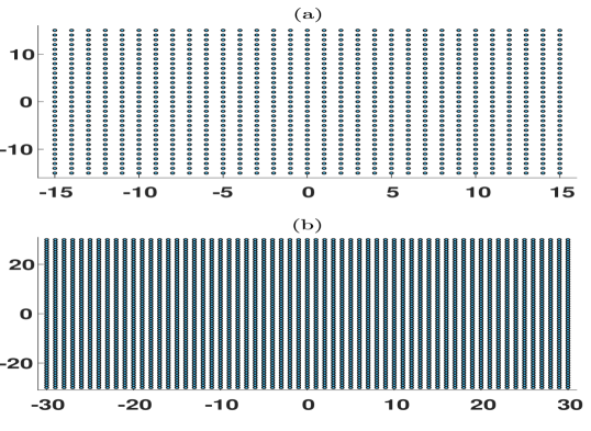
Figure 2: (a) A uniform planar array of $31^{2}=961$ physical elements and (b) the corresponding sum co-array with $61^{2}=3721$ virtual elements. Each circle represents an array element.

Definition 3.

Intrinsic Apodization: Consider a planar array $E$ and define a binary indicator matrix $\bf I$ whose entries are ${\bf I}[n,m]=1$ if $(n,m)\in E$ and zero otherwise. The intrinsic apodization of $E$ is an integer matrix defined as

$${\bf A}_{E}\triangleq{\bf I}\ast{\bf I},$$ (13)

where $\ast$ denotes 2D convolution operation. Alternatively, the entries $a_{E}[n,m]$ of ${\bf A}_{E}$ can be written as

$$\small a_{E}[n,m]=\left|\Big{\{}\Big{(}(u,v),(k,l)\Big{)}\in E^{2}:u+k=n,v+l=m\Big{\}}\right|.$$ (14)

The sum co-array and the intrinsic apodization play important roles as they directly affect image quality. As we later demonstrate, the former dictates the size/support of the effective aperture created by COBA-3D, while the latter determines the weights of this aperture.

III-B 3D Convolutional Beamforming

Now, we introduce COBA-3D which extends convolutional beamforming [71] to 3D settings with diverging wave transmission. We include an analysis of the consequent sum co-array and receive beam pattern, leading to improved image quality. We note that although the beamforming process is performed digitally, we use in the following the continuous time notation $t$ to simplify the presentation.

Consider imaging with a UPA $E$ where we transmit a series of $K$ diverging-waves with inclination angles $\{\alpha_{k},\beta_{k}\}_{k=0}^{K}$ and record the reflected echoes following each transmission. Upon reception, IQ sampling is first performed at a sampling rate at least as high as the Nyquist rate [40, 81] determined by the transducer center frequency. To achieve a posteriori synthetic transmit focusing, we coherently compound [82] the complex received signals by applying to each signal appropriate time delays depending on the element positions and the desired direction $(\theta_{0},\phi_{0})$. Then, we sum (compound) the results over all transmissions to obtain the compound signal, given by

$$y_{n,m}(t)\triangleq\sum_{k=0}^{K}f_{n,m,\alpha_{k},\beta_{k}}(t+\gamma_{n,m,\alpha_{k},\beta_{k}}),$$ (15)

where $f_{n,m,\alpha_{k},\beta_{k}}$ denotes the signal received by the element $(n,m)$ following the transmission with inclination angles $\{\alpha_{k},\beta_{k}\}$, and $\gamma_{n,m,\alpha_{k},\beta_{k}}$ is the corresponding time delay (please refer to Chapter I.B of [83]). Note that the time-point $t$ in (15) is proportional to the desired axial depth $z$ via $z=\frac{ct}{2}$.

Next, for any $n\in[-N,N]$ and $m\in[-M,M]$, we define the following signals where $|\cdot|$ and $\phase{\cdot}$ are the modulus and phase of the signal respectively. Denoting by ${\bf r}(t)$ the matrix whose entries are $r_{n,m}(t)$, we define for each time-point the convolution signal

$${\bf c}(t)=({\bf r}\ast{\bf r})(t),$$ (16)

where $\ast$ denotes 2D spatial convolution. The matrix ${\bf c}(t)$ is of size $(4N+1)\times(4M+1)$ and can be computed efficiently using a spatial 2D-FFT and its inverse 2D-IFFT as

$${\bf c}(t)=\text{2D-IFFT}\Big{\{}\text{2D-FFT}\{{\bf r}\}\odot\text{2D-FFT}\{{\bf r}\}\Big{\}}(t),$$ (17)

where $\odot$ represents the Hadamard product. The signal, beamformed at direction $(\theta_{0},\phi_{0})$, is then obtained by summing all the entries of ${\bf c}(t)$

$$b(t)\triangleq\sum_{n=-2N}^{2N}\sum_{m=-2M}^{2M}\tilde{w}_{R}[n,m]{\bf c}_{n,m}(t),$$ (18)

where $\{{\bf c}_{n,m}(t)\}$ are the entries of ${\bf c}(t)$ and $\tilde{w}_{R}[n,m]$ are the weights (apodization) applied to the convolution signal. To attain an effective apodization of $w_{R}[n,m]$, the actual weights should be set as

$$\tilde{w}_{R}[n,m]=\frac{w_{R}[n,m]}{a_{E}[n,m]},$$ (19)

accounting for the intrinsic apodization $a_{E}[n,m]$ given by (14) that stems from the convolution operation.

The dimension (length) of the vector $b(t)$ and the number of such scan-lines are determined by the discretization along depth (time) and number of chosen directions $(\theta,\phi)$, which represent the underlying grid of the reconstructed image. Finally, collecting all beamformed signals $b(t)$ of all directions allows to compose the complete volumetric image defined over a predetermined 3D grid where any region of interest within it is available for visualization.

We summarize COBA-3D in Algorithm 1. We note that here we utilize diverging-waves, however, COBA-3D can be performed with focused transmission or any other unfocused insonification such as plane waves. When focused mode is utilized, the first stage of compounding is skipped since focusing is performed upon transmission.

Algorithm 1 COBA-3D

0:  IQ signals $\{f_{n,m,\alpha,\beta}(t)\}$, weights $\{w_{R}[n,m]\}$.

  1: Perform coherent compounding

$$y_{n,m}(t)=\sum_{k=0}^{K}f_{n,m,\alpha_{k},\beta_{k}}(t+\gamma_{n,m,\alpha_{k},\beta_{k}})$$

  2: Compute $r_{n,m}(t)=\exp\{j\phase{y_{n,m}(t)}\}\sqrt{|y_{n,m}(t)|}$

  3: Perform 2D convolution using 2D FFT

$${\bf c}(t)=\text{IFFT}\Big{\{}\text{FFT}\{{\bf r}\}\odot\text{FFT}\{{\bf r}\}\Big{\}}(t)$$

  4: Set weights $\tilde{w}_{R}[n,m]=\frac{w_{R}[n,m]}{a_{E}[n,m]}$

  5: Calculate the beamformed signal

$$b(t)\triangleq\sum_{n=-2N}^{2N}\sum_{m=-2M}^{2M}\tilde{w}_{R}[n,m]{\bf c}_{n,m}(t)$$

  Beamformed signal $b(t)$.

In the Appendix we analyze the receive beam pattern created by COBA-3D, leading to the following expression

$$\begin{split}H_{RX}(\theta,\phi)&=\sum_{(n,m)\in S_{E}}w_{R}[n,m]e^{-j(s_{x}n+s_{y}m)}\\ &=\sum_{n=-2N}^{2N}\sum_{m=-2M}^{2M}w_{R}[n,m]e^{-j(s_{x}n+s_{y}m)}\end{split}$$ (20)

where $w_{R}[\cdot,\cdot]$ are the effective receive weights. As can be seen, the receive beam pattern is directly related to the sum co-array whose aperture is larger than that of the physical array. The latter leads to a receive beam pattern with narrower main lobe and lower side lobes in comparison to DAS as demonstrated in Fig. 3. Furthermore, for appropriate choice of the inclination angles, coherent compounding effectively generates a posteriori synthetic focusing in the transmission [82], thus creating a transmit beam pattern $H_{TX}(\theta,\phi)$ that is similar to or even better than that achieved by standard focused transmissions. Thus, COBA-3D leads to an overall beam pattern of $H_{COBA-3D}(\theta,\phi)=(H_{TX}\cdot H_{RX})(\theta,\phi)$ which is superior to that created by DAS, and thus it should theoretically result in enhanced image quality. This result is verified by practical experiments in Section IV.

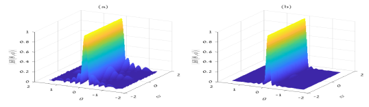
Figure 3: Receive beam patterns: (a) DAS and (b) COBA-3D. Both beamformers use unity receive weights.

The resultant algorithm COBA-3D resembles COBA presented in [71] but differs from it in three major aspects. First, we add a preprocessing step of compounding which allows COBA-3D to handle unfocused transmissions and increase frame rate. COBA considers focused transmission which limits the frame rate due to the large number of required scan-lines that can reach several tens of thousands in a 3D setup. On the other hand, the frame rate achieved by COBA-3D is dictated by the number of inclination angles $K$ which is typically one order of magnitude lower than the number of scan-lines required in focused imaging, thus enabling real-time imaging. Second, COBA-3D operates on IQ signals which removes the need to perform post band-pass or high-pass filtering. As explained in [71], when RF data is used the spatial convolution leads to undesired low frequency components that need to be filtered out. The latter side effect is avoided when IQ data is used, thus, removing the post filtering step of COBA. Last and most important, COBA-3D recovers volumetric data and thus reduces operator dependency in the imaging process. Once the 3D data is obtained, any view of any region within it can be displayed without operating the probe, including complete views of anatomical body structures that are are intrinsically 3D such as the mitral valve. Moreover, the volume data provides exact location and orientation information, thus, a variety of parameters can be estimated from a 3D image in a more accurate and reproducible fashion compared to 2D imaging [84, 85, 86].

To conclude this part, COBA-3D allows to handle diverging wave transmissions, thus, obtaining ultrafast frame rate. In addition, it generated an improved receive beam pattern which potentially should lead to higher image quality than DAS. A challenge that remains is the heavy receive hardware and the corresponding sizable data that needs to be processed upon reception due to the large number of receive elements.

III-C Sparse Beamforming

So far, we introduced COBA-3D which is designed to achieve ultrafast frame rate and improved image resolution and contrast compared to DAS. However, still a large number of receive elements is required, leading to high cost, power and computational burden. Moreover, the latter increases considerably when transmitting diverging-waves, since the entire region of interest is reconstructed following each transmission (and not a single scan-line).

To obtain element reduction without degrading performance in terms of image resolution and contrast, we utilize 2D sparse arrays defined next. This is a generalization of the sparse arrays introduced in [71] to the 2D setting.

Definition 4.

2D Sparse Array: Let $E$ and $T$ be two planar arrays, and denote by $S_{T}$ the sum co-array of $T$. We say $T$ is a sparse (or thinned) array with respect to $E$ if

$$T\subset E\subseteq S_{T},$$ (21)

where in the above we consider the elements sets of the arrays.

Suppose we perform imaging by using a UPA $E$ for transmitting tilted diverging-waves where upon reception we employ a thinned (sparse) array $T$ for acquiring the backscattered signals. We can no longer compute $b(t)$ as in (16) or (17) since we removed some of the elements (or signals). Therefore, we compute the convolution signal $\textbf{c}(t)$ using pair-wise multiplications of the signals as follows. Denoting by $S_{T}$ the sum co-array of $T$, for any $(n,m)\in S_{T}$ we define

$$c_{n,m}(t)=\sum_{(u,v)\in T}\;\sum_{\begin{subarray}{c}(k,l)\in T:\\ u+k=n\\ v+l=m\end{subarray}}(r_{u,v}\cdot r_{k,l})(t).$$ (22)

Alternatively, we can obtain (22) by filling in the missing signals with zeros and then performing a 2D convolution

$${\bf c}(t)=(\tilde{\bf r}\ast\tilde{\bf r})(t),$$ (23)

where

$$\tilde{r}_{n,m}(t)=\begin{cases}r_{n,m}(t),\;&(n,m)\in T,\\ 0,\;&\text{otherwise.}\end{cases}$$ (24)

Finally, the beamformed signal is given by

$$b(t)=\sum_{(n,m)\in S_{T}}\tilde{w}_{R}[n,m]c_{n,m}(t),$$ (25)

where we incorporated the receive aperture function $\tilde{w}_{R}[n,m]$, determined by considering the intrinsic apodization of the sparse array $T$ as in (19). Again, this process yields a single scan line $b(t)$ of a specific direction and should be repeated for all desired directions to obtain the complete 3D image. The resultant technique, referred as sparse COBA-3D (SCOBA-3D), is outlined in Algorithm 2.

Algorithm 2 SCOBA-3D

0:  IQ signals $\{f_{n,m,\alpha,\beta}(t)\}$, weights $\{w_{R}[n,m]\}$.

  1: Perform coherent compounding

$$y_{n,m}(t)=\sum_{k=0}^{K}f_{n,m,\alpha_{k},\beta_{k}}(t+\gamma_{n,m,\alpha_{k},\beta_{k}})$$

  2: Compute $r_{n,m}(t)=\exp\{j\phase{y_{n,m}(t)}\}\sqrt{|y_{n,m}(t)|}$

  3: Calculate $c_{n,m}(t)$ using (22) or (23) for all $(n,m)\in S_{T}$

  4: Set weights $\tilde{w}_{R}[n,m]=\frac{w_{R}[n,m]}{a_{T}[n,m]}$ for all $(n,m)\in S_{T}$

  5: Compute the beamformed signal using (25)

$$b(t)=\sum_{(n,m)\in S_{T}}\tilde{w}_{R}[n,m]c_{n,m}(t)$$ (26)

  Beamformed signal $b(t)$.

Following the same steps as in the Appendix, we can obtain an expression of the receive beam pattern created by SCOBA-3D

$$H_{RX}(\theta,\phi)=\sum_{(n,m)\in S_{T}}w_{R}[n,m]e^{-j(s_{x}n+s_{y}m)}$$ (27)

where $w_{R}[n,m]$ are the effective apodization and $a_{T}[n,m]$ are the intrinsic apodization of $T$ defined in (14). By Definition 21, we have that $E\subset S_{T}$, hence, we can write

$$\begin{split}H_{RX}(\theta,\phi)&=\sum_{(n,m)\in E}w_{R}[n,m]e^{-j(s_{x}n+s_{y}m)}\\ &+\sum_{(n,m)\in S_{T}/E}w_{R}[n,m]e^{-j(s_{x}n+s_{y}m)},\end{split}$$ (28)

where $S_{T}/E\triangleq\left\{(n,m)\in S_{T}:\,(n,m)\notin E\right\}$. Therefore, condition (21) ensures that the resultant sum co-array exhibits at least as large aperture as that of the fully-populated array $E$. In the special case where we set $w_{R}[n,m]=0$ for all $(n,m)\in S_{T}/E$, expression (27) reduces to

$$H_{RX}(\theta,\phi)=\sum_{(n,m)\in E}\hat{w}_{R}[n,m]e^{-j(s_{x}n+s_{y}m)},$$ (29)

which is the receive beam pattern achieved by DAS operating on the full array $E$. Hence, SCOBA-3D provides more degrees of freedom in choosing the apodization weights than DAS. Finally, since we remove elements only upon reception, the transmit beam pattern remains unchanged, as before.

Fig. 4 presents examples of various sparse arrays and their corresponding sum co-arrays. All sum co-arrays in this case includes a UPA within them. A special case is the ’X’-shape array whose sum co-array contains a tilted UPA. As seen, the use of sparse geometries offers a dramatic reduction in the number of elements, leading to a number of elements typically used for 2D imaging. In addition, different sparse arrays lead to different intrinsic apodization weights as shown in Fig. 5. Some intrinsic apodization functions can improve image quality, e.g. Fig. 5(a) which reduces side lobes, while others exhibit discontinuities due to zero weights that might lead to an adverse effect on the beam pattern. Therefore, any choice of receive weights has to consider the intrinsic apodization caused by the spatial convolution.

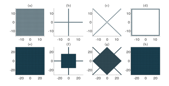
Figure 4: Sparse Arrays: (a) the original UPA - 961 elements, (b) ’$+$’-shape array - 61 elements, (c) ’X’-shape array - 61 elements , (d) ’$\Box$’-shape array - 120 elements. (e)-(h) are the corresponding sum co-arrays with 3721, 1021, 1021 and 3721 elements respectively. Each circle represents an array element. All sum co-arrays contains within them a UPA which in turn includes the original UPA.

Figure 5: Intrinsic apodization of various arrays: (a) UPA, (b) ’$+$’-shape array, (c) ’X’-shape array, (d) ’$\Box$’-shape array. Any choice of sparse array leads to different intrinsic apodization that can improve or degrade image quality. Hence, the intrinsic apodization should be considered when setting the receive weights.

III-D Fractal Array Design

Sparse arrays play a major role in convolutional beamforming. Besides the number of physical elements, there are additional important design criteria for sparse arrays that affect the performance. Examples are:

Criterion 1 (Closed-form).

To allow scalability, elements locations should be given in closed-form.

Criterion 2 (Symmetric Array).

Consider a planar array $T$ and denote by $\hat{T}$ a version of the array rotated by $180^{\circ}$:

$$\hat{T}\triangleq\{(-n,-m)\,|\;(n,m)\in T\}.$$

A planar array $T$ is symmetric if $T=\hat{T}$.

Criterion 3 (Full Sum Co-Array).

Consider a planar array $T$ whose sum co-array is $S_{T}$. The sum coarray $S_{T}$ is said to be full (i.e. contiguous) if it is a UPA. This ensures that the aperture of the sum co-array does not exhibit discontinuities which may have adverse effect on the beam pattern.

Criterion 4 (Large Sum Co-Array).

To obtain considerable element reduction, the sum co-array $S_{T}$ of a sparse array $T$ should satisfy $\left|S_{T}\right|=\mathcal{O}(\left|T\right|^{2})$ [87]. This implies that the aperture size of the sum co-array is large, leading to improved resolution and contrast.

Depending on the specific application, one may consider additional array properties of interest such as mutual coupling (element cross-talk) [73], but for simplicity we focus here on the criteria mentioned above, as we did in [73].

When considering these criteria, the design of sparse arrays becomes intractable in large scale, i.e., when the number of elements is large as in 3D imaging. To address this issue, we adopt recent work [72, 73] and extend it to introduce a 2D fractal array design based on the sum co-array.

Consider a planar array $T$ whose sum co-array $S_{T}$ is assumed to be full. We propose the following recursive array definition for any natural number $r$

$$\begin{split}&{F}_{0}\triangleq\{0\},\\ &{F}_{r+1}\triangleq\bigcup_{(n,m)\in{T}}\left({F}_{r}+(n\cdot C_{x}^{r},\,m\cdot C_{y}^{r})\right),\end{split}$$ (30)

where $C_{x}$ and $C_{y}$ are the number of elements in each row and column of $S_{T}$, respectively. Note that $T$, referred to as the generator [72], satisfies $T=F_{1}$. Each fractal array $F_{r+1}$ is composed of $\left|T\right|$ replicas of $F_{r}$ arranged in space according to $T$, leading to a total number of elements of $\left|T\right|^{r}$ in $F_{r}$. Fig. 6 exemplifies the proposed fractal design where we choose the generator to be a UPA.

In [72], a similar fractal array definition was proposed based on the difference co-array rather than the sum co-array as in our scheme. However, for symmetric arrays the sum and difference co-arrays are identical. Therefore, for a symmetric generator, the theoretical proofs derived in [72] apply to our case, implying that the fractal arrays inherit the properties of their generator. In particular, whenever the generator satisfies Criteria 2-4 so do its fractal expansions. Thus, the fractal scheme (30) provides a simple systematic way for designing sparse arrays by constructing a generator array with desirable properties (using e.g. exhaustive search) and then enlarging it recursively while preserving its properties, as shown in Fig. 6.

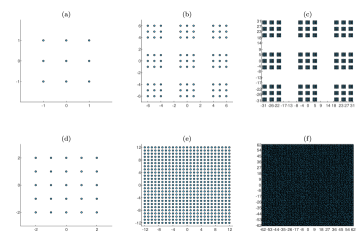
Figure 6: Fractal Arrays: (a) The generator array with 9 elements and its fractal extensions (b) $F_{2}$ and (c) $F_{3}$ with 81 and 729 elements respectively. The corresponding sum co-arrays are given in (d), (e) and (f) with 25, 625 and 15625 elements respectively.

IV Evaluation Results

Here we study the performance of 3D convolutional beamforming operating on thinned receive arrays and compare it to standard DAS applied on the full array. We present experiments performed with the parallelized Verasonics systems at the University of Lyon [5] where we consider either focused transmission scheme or diverging-wave compounding. First, we present images of phantom scans and examine them to assess image resolution and contrast qualitatively and quantitatively. Then, we show results obtained from ex-vivo data to strengthen our validation. In the following, we refer in this section for brevity to COBA-3D and SOCBA-3D as COBA and SCOBA respectively. We begin with a full description of our experimental setup.

IV-A System description

The acquisition system consists of four Vantage 256 systems (Verasonics, USA) which are synchronized together with an external box (Verasonics, USA). Such a configuration allows controlling 1024 individual channels in both transmission and reception. A 2D probe is connected to the systems, each of them driving 256 elements. The probe is composed of 32 $\times$ 35 elements with a 300 $\mu$m pitch in both $x$ and $y$ direction (Vermon, France). We note that in the $y$ direction, elements line #9, #17, and #25 are not connected [5]. For both focused and diverging-wave transmissions, a 2-cycle 3-MHz sinusoidal wave is transmitted into the medium. The reception is conducted with a 12 MHz sampling frequency.

The difference between the two transmission schemes concerns the position of the focal spot, which is a positive $z$ value in the focalized transmissions and a negative $z$ value for diverging-waves. For the focalized emissions, the focal spot is initially set at 40 mm depth. Then, steering is applied in both elevation ($xz$ plane) and azimuth ($yz$ plane). In both directions, the angle value are in the range [-30^∘; 30^∘], discretized in 49 and 51 angles for elevation and azimuth direction, respectively. This leads to 2499 transmission/reception events. For diverging-waves, the virtual focal spot is located at -4.8 mm, which is half the probe aperture. Then, steering is applied in both planes in the range [-10^∘; 10^∘] with a discretization of 9 angles in both direction, leading to a total of 81 transmission/reception events.

Throughout the experiments we use the full aperture for transmission, whereas upon reception we utilize sparse arrays by removing (ignoring) part of the elements out of the full $31\times 31$ aperture. The chosen arrays, shown in Fig. 7, are non-fractal arrays based on nested arrays [88, 71] and were selected since they are simple to construct and their sum co-arrays contain a UPA. Moreover, the different thinned configurations allow to easily display various levels of element reduction and the effect on the size of the UPA contained in the corresponding sum co-arrays. The sum co-arrays lead to different beam patterns as given in Fig. 7, leading to different image qualities as we later demonstrate in this section. For clarity, the sparse arrays (b), (c) and (d) of Fig. 7 are denoted as Array I, II and III respectively. We apply DAS and COBA on the UPA of Fig. 7 and SCOBA on Arrays I, II and III where we refer to the resultant methods as SCOBA I, II and III accordingly. In addition, no apodization is applied in any of the methods examined for fair comparison.

The proposed fractal design aims at constructing large sparse array. Here, due to our available system setup, we are confined to a $31\times 31$ aperture that is considered to be small for our purposes, thus, limiting us in showing the full extent of our recursive array scheme. However, for completeness of our work, we provide additional results obtained using the sparse fractal array in Fig. 6(b) which consists of 81 out of 169 ($13\times 13$) elements comprising the full counterpart array. Note that this fractal array satisfies Criteria 1-3, but not Criterion 4 since its generator fails to meet it, as seen from Fig. 6(a) and Fig. 6(d). As a proper comparison, we present results obtained with DAS operating on the full $13\times 13$ array with either focused or diverging wave transmission.

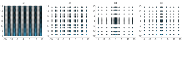
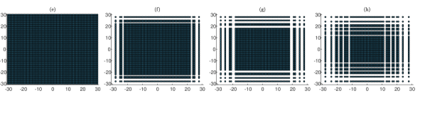
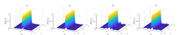
Figure 7: Array Configurations: (a) UPA with 961 elements, (b)-(d) sparse arrays with 225, 169 and 121 elements respectively. The corresponding sum co-arrays are shown in (e)-(h) and the respective beam patterns, exhibited by SCOBA, are given in (i)-(l).

IV-B Phantom Experiments

First, both transmission schemes are used on a commercial grayscale phantom (Gammex Sono410 model). We start with focused transmission. Fig. 8 provides various images obtained by the different beamforming techniques. The images include a anechoic cyst which is used to visually assess the contrast of the recovered images. Examining the cyst, we can see that COBA generates sharper images than DAS. SCOBA achieves similar or improved contrast in comparison to DAS while offering 4-8 fold element reduction upon reception. A closer look at the performance of the beamformer is shown in Fig. 9 where we display cross-sections of the cyst to visually assess contrast. As a quantitative measure, we compute the contrast ratio (CR) [89]

$$\text{CR}=20\log_{10}\left(\frac{\mu_{\text{cyst}}}{\mu_{bck}}\right)$$ (31)

where $\mu_{\text{cyst}}$ and $\mu_{\text{bck}}$ are the mean image intensities, prior to log-compression, computed over two regions inside the cyst and in the surrounding background, respectively. The chosen regions are marked by dashed red circles in Fig. 9. The results, given in Table I, show that COBA exhibits enhanced image contrast as well as SCOBA variants comapred to DAS

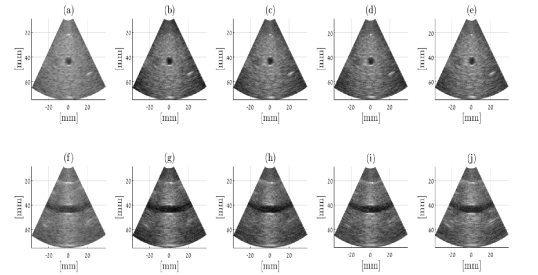
Figure 8: Orthogonal views of (top) $xz$ and (bottom) $yz$ planes of a Gammex phantom with anechoic cyst obtained using focused transmission with DAS (961), COBA (961), SCOBA I (225), SCOBA II (169), and SCOBA III (121) in their respective order from left to right. Numbers in brackets refer to the number of receive elements. Images are displayed with a dynamic range of 90dB.

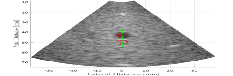
(a)

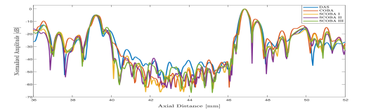
(b)

Figure 9: (a) The red circles mark the areas used for computing the CR values of Table I, while the dashed green line indicates the location of the cross-section shown in (b) to evaluate contrast.

TABLE I: CR [dB].
The numbers in brackets denote the number of receive elements.

	DAS (961)	COBA (961)	SCOBA I (225)	SCOBA II (169)	SCOBA III (121)
Focused	-23.97	-30.60	-30.57	-30.71	-27.86
DW	-7.38	-10.20	-9.70	-8.69	-6.52

Now, we study the resolution of the obtained images. To that end, we use phantom images which comprise point targets. Examining the results in in Fig 10, specifically the points scatterers, we can see that COBA and SCOBA variants provide improved resolution compared to DAS. This is result strengthens when cross-section of a chosen point scatterer is displayed in Fig. 11, showing the variants of SCOBA yield better resolution than DAS and COBA outperforms them all. In addition, we compute the full-width at half-maximum (FWHM) to quantitatively measure the resolution obtained by each method. The results are given in Table II, emphasizing the enhanced resolution offered by the proposed beamforming algorithms.

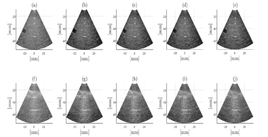
Figure 10: Orthogonal views of (top) $xz$ and (bottom) $yz$ planes of a Gammex phantom with punctual targets obtained using focused transmission with (a) DAS (961), (b) COBA (961), (c) SCOBA I (225), (169) SCOBA II and SCOBA III (121). Numbers in brackets refer to the number of receive elements. Images are displayed with a dynamic range of 90dB.

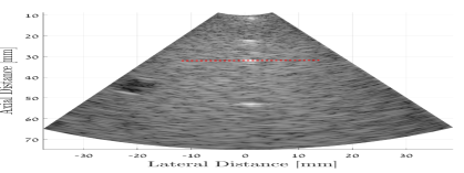
(a)

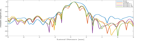
(b)

Figure 11: (a) The dashed red line marks the location of the cross-section shown in (b) to assess resolution.

TABLE II: FWHM [mm].
The numbers in brackets denote the number of receive elements.

	DAS (961)	COBA (961)	SCOBA I (225)	SCOBA II (169)	SCOBA III (121)
Focused	1.89	0.94	0.94	0.94	0.94
DW	2.65	1.36	1.68	1.76	1.84

Next, we examine the proposed techniques when diverging-wave transmission is used to achieve high frame-rate. In Fig. 12, we present images of anechoic cyst, acquired with unfocused insonification and recovered by performing coherent compounding upon reception. These results along with the cross-sections shown in Fig. 13 prove that the proposed techniques are suitable for diverging-wave transmission. COBA clearly demonstrates better contrast than DAS, while all variants of SCOBA outperform DAS in terms of contrast where their performance increases with the number of elements. The CR values given in Table I verify these conclusions.

To estimate image resolution, we show additional images in Fig. 14 which include point targets. The cross-section presented in Fig. 15 displays the resolution improvement obtained by COBA and the selected versions of SCOBA. These results are supported quantitatively by the FWHM values in Table II.

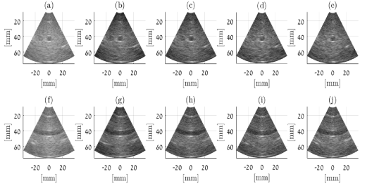
Figure 12: Orthogonal views of (top) $xz$ and (bottom) $yz$ planes of a Gammex phantom with anechoic cyst obtained using diverging-waves with DAS (961), COBA (961), SCOBA I (225), SCOBA II (169), and SCOBA III (121) in their respective order from left to right. Numbers in brackets refer to the number of receive elements. Images are displayed with a dynamic range of 80dB.

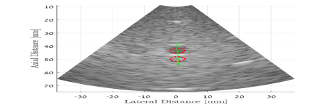
(a)

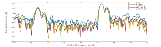
(b)

Figure 13: (a) The red circles point to the areas used for computing the CR values of Table I, while the dashed green line marks the location of the cross-section shown in (b) to assess contrast.

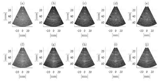
Figure 14: Orthogonal views of (top) $xz$ and (bottom) $yz$ planes of a Gammex phantom with punctual targets obtained using diverging-waves with DAS (961), COBA (961), SCOBA I (225), SCOBA II (169), and SCOBA III (121) in their respective order from left to right. Numbers in brackets refer to the number of receive elements. Images are displayed with a dynamic range of 80dB.

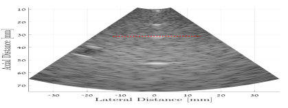
(a)

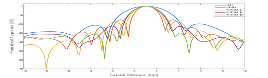
(b)

Figure 15: (a) The dashed red line indicates the location of the cross-section shown in (b) to assess resolution.

We complete this part by demonstrating the use of our recursive shceme where we expand a nine element UPA to create the fractal array $F_{2}$ shown in Fig. 6(b). The fractal sparse array is utilized to perform 3D imaging with either focused transmission or diverging-wave compounding where we apply SCOBA upon reception. Fig. IV-B displays resultant images as well as images recovered by DAS operating on a $13\times 13$ element array (full receive aperture). Assessing the images visually, one can see that use of the fractal array led to images that exhibit better resolution and contrast compared to those created by DAS, while utilizing fewer than half of the receive elements (81 out 169). These results show the simplicity and efficiency of the proposed fractal design and its in performing sparse beamforming. Note that the images of Fig. IV-B are of low quality compared to the previous results which is expected since here we use a considerably smaller aperture upon reception.

Figure 16: Images of the $xz$ (left) and $yz$ (right) plane of a Gammex phantom acquired using a 161 ($13\times 13)$ element UPA with either focused transmission (top) or diverging waves (bottom). Upon reception, we applied DAS on the full receive array to produce images (a), (c), (e) and (g). The other images, (b), (d), (f) and (h), were obtained by SCOBA operating on a 81 element fractal receive array shown in Fig. 6(b). Images are displayed with a dynamic range of 80dB.

IV-C Ex-vivo Experiments

Finally, ex vivo acquisitions were performed, scanning a lamb kidney. This medium has a typical external shape and it also exhibits, in its internal structure, characteristics that should be found in 3D ultrasound imaging (e.g. vascularization). To properly assess the proposed beamforming strategy for ex vivo acquisitions, we maintain the same transmission/reception settings as before. Given the size of the imaged tissues, the probe has been placed in order to scan the larger possible section of each medium. Fig. 17 presents various results acquired using focused transmission while Fig. 18 displays images obtained with diverging-wave compounding. It can be seen from the results that COBA and SCOBA yield images with higher contrast than DAS. Examining the images of Fig. 18, we can clearly observe the improvement in resolution achieved by COBA and SCOBA. Thus, these images provide a strong evidence that the proposed techniques outperform DAS. SCOBA variants offer similar or better image quality than DAS while allowing a 4-8 fold element reduction, thus, enabling high-quality 3D ultrasound imaging.

We end the experiments with last results obtained using the fractal array of Fig. 6(b). The generated images are shown in Fig. 19 in comparing to DAS as before. Theses results show the applicability of our recursive array design with SCOBA, leading to improved performance, superior to DAS, where we use significantly fewer elements than DAS without compromising image quality.

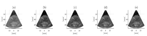
Figure 17: Images of the $xz$ plane of a lamb kidney using focused transmission with DAS (961), COBA (961), SCOBA I (225), SCOBA II (169), and SCOBA III (121) in their respective order from left to right. Numbers in brackets refer to the number of receive elements. Images are displayed with a dynamic range of 80dB.

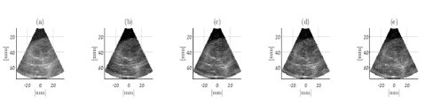
Figure 18: Images of the $xz$ plane of a lamb kidney obtained using diverging-waves with DAS (961), COBA (961), SCOBA I (225), SCOBA II (169), and SCOBA III (121) in their respective order from left to right. Numbers in brackets refer to the number of receive elements. Images are displayed with a dynamic range of 80dB.

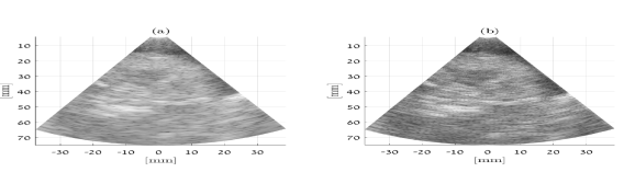
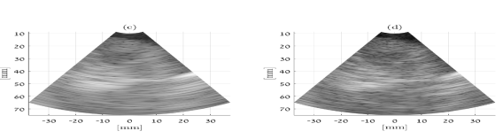
Figure 19: Images of the $xz$ plane of a lamb kidney. (a) and (c) are images obtained by DAS operating on a 161 ($13\times 13)$ element receive UPA with focused and diverging wave transmission respectively. (b) and (d) are images obtained by SCOBA operating on a 81 element fractal receive array (Fig. 6b) with focused and diverging wave transmission respectively.

V Conclusion

In this work we introduced COBA-3D which extends the notion of convolutional beamforming to the 3D setting with unfocused insonification. The key part of COBA-3D is the 2D spatial convolution of the received signals, computed efficiently in the Fourier domain. This results in improved image resolution and contrast in comparison to DAS. We relate this improvement in image quality to the virtual sum co-array which is larger than the physical array and thus yields an enhanced receive beam pattern. Furthermore, we presented SCOBA-3D which exploits sparse arrays whose sum co-arrays are large to perform 3D imaging with a notable 4-8 fold element reduction upon reception. To complete our approach, we introduced a fractal design which expands recursively a generator array with favorable properties to create an arbitrarily large sparse array with the same properties. This design facilities the construction of sparse arrays with multiple desired properties and its impact should increase as technology advances and the number of elements grows.

To assess the performance of our proposed techniques, we performed various experiments on phantom scans, including focused and diverging-wave transmissions. The qualitative and quantitative results verify that COBA-3D achieves improved image resolution and contrast in comparison to DAS. In additions, SCOBA-3D enables to generate high-quality 3D images with a small number of receive elements, typically found in 1D probes. Similar results were obtained in ex-vivo experiments, validating the proposed methods.

To summarize, convolutional beamforming for 3D imaging offers enhanced image quality in terms of both resolution and contrast. Moreover, it can be easily combined with unfocused insonification, such as diverging-wave compounding, to allow ultrafast frame rate. Finally, our fractal array design complements the proposed beamforming by allowing to construct sparse arrays where the majority of receive electronics are discarded. Thus, we reduce the processing rate, cost and power, facilitating the use of high-performance 3D US imaging with limited hardware.

Appendix A Receive Beam Pattern Analysis

Here we derive an expression of the receive 2D beam pattern created by COBA-3D. The following can be seen as an extension to 2D of the beam pattern analysis given in [71].

Assume the input signal is $f(t)=e^{j\omega_{0}t}$ impinging on the array at some direction $(\theta_{0},\phi_{0})$. Thus, we obtain

$$r_{n,m}(t)=e^{j\omega_{0}t}e^{-j\omega_{0}\tau_{n,m}},$$ (38)

where $\tau_{n,m}$ is defined in (4). The beamformed signal can be expressed as

$$b(t)=\sum_{(u,v)\in E}\,\sum_{(k,l)\in E}(r_{u,v}\cdot r_{k,l})(t).$$ (39)

Notice that

$$(r_{u,v}\cdot r_{k,l})(t)=e^{j\omega_{0}t}r_{u+k,v+l}(t).$$ (40)

Therefore, we get

$$b(t)=\sum_{(n,m)\in S_{E}}\tilde{w}_{R}[n,m]a_{E}[n,m]e^{j\omega_{0}t}r_{n,m}(t),$$ (41)

where $\tilde{w}_{R}[n,m]$ is the receive apodization weights, $S_{E}$ is the sum co-array of $E$ and $a_{E}[n,m]$ are the corresponding intrinsic apodization given by (14). Substituting (38) into (41), we obtain

$$b(t)=e^{j2\omega_{0}t}\sum_{(n,m)\in S_{E}}w_{R}[n,m]e^{-j\omega_{0}\tau_{n,m}}.$$ (42)

where we define $w_{R}[n,m]\triangleq\tilde{w}_{R}[n,m]a_{E}[n,m]$. Notice that the weights $\tilde{w}_{R}[n,m]$ should consider the intrinsic apodization to obtain a desired effective apodization $w_{R}[n,m]$.

Consequently, the receive beam pattern of COBA-3D is

$$H_{COBA-3D}(\theta,\phi)=\sum_{(n,m)\in S_{E}}w_{R}[n,m]e^{-j(s_{x}n+s_{y}m)}$$ (43)

where $s_{x}$ and $s_{y}$ are given by (9). The resultant beam pattern depends on the sum co-array and the intrinsic apodization. When the physical array $E$ is a UPA, then $S_{E}$ is another UPA of twice the aperture size in both axes. A larger aperture implies better image resolution. Moreover, it increases the degrees of freedom in determining the apodization. Hence, an appropriate choice of the weights, which accounts for the intrinsic apodization, can lead to effective weights such as Hamming apodization that enhance image contrast.

References

- [1] A. Fenster and J. C. Lacefield, Ultrasound imaging and therapy. Taylor & Francis, 2015.
- [2] K. E. Thomenius, “Evolution of ultrasound beamformers,” in Proceedings of Ultrasonics Symposium., vol. 2. IEEE, 1996, pp. 1615–1622.
- [3] M. Karaman, P.-C. Li, and M. O’Donnell, “Synthetic aperture imaging for small scale systems,” IEEE Transactions on Ultrasonics, Ferroelectrics, and Frequency Control, vol. 42, no. 3, pp. 429–442, 1995.
- [4] A. Eklund, P. Dufort, D. Forsberg, and S. M. LaConte, “Medical image processing on the GPU: Past, present and future,” Medical Image Analysis, vol. 17, no. 8, pp. 1073–1094, 2013.
- [5] L. Petrusca, F. Varray, R. Souchon, A. Bernard, J.-Y. Chapelon, H. Liebgott, W. N’Djin, and M. Viallon, “Fast volumetric ultrasound B-mode and Doppler imaging with a new high-channels density platform for advanced 4D cardiac imaging/therapy,” Applied Sciences, vol. 8, no. 2, p. 200, 2018.
- [6] J. A. Jensen, H. Holten-Lund, R. T. Nilsson, M. Hansen, U. D. Larsen, R. P. Domsten, B. G. Tomov, M. B. Stuart, S. I. Nikolov, M. J. Pihl et al., “SARUS: A synthetic aperture real-time ultrasound system,” IEEE Transactions on Ultrasonics, Ferroelectrics, and Frequency Control, vol. 60, no. 9, pp. 1838–1852, 2013.
- [7] J. Provost, C. Papadacci, C. Demene, J.-L. Gennisson, M. Tanter, and M. Pernot, “3-D ultrafast Doppler imaging applied to the noninvasive mapping of blood vessels in Vivo,” IEEE Transactions on Ultrasonics, Ferroelectrics, and Frequency Control, vol. 62, no. 8, pp. 1467–1472, 2015.
- [8] B. Savord and R. Solomon, “Fully sampled matrix transducer for real time 3D ultrasonic imaging,” in Symposium on Ultrasonics., vol. 1. IEEE, 2003, pp. 945–953.
- [9] D. Wildes, W. Lee, B. Haider, S. Cogan, K. Sundaresan, D. M. Mills, C. Yetter, P. H. Hart, C. R. Haun, M. Concepcion et al., “4D ICE: A 2D array transducer with integrated ASIC in a 10-Fr catheter for real-time 3D intracardiac echocardiography,” IEEE Transactions on Ultrasonics, Ferroelectrics, and Frequency Control, vol. 63, no. 12, pp. 2159–2173, 2016.
- [10] P. Santos, G. U. Haugen, L. Løvstakken, E. Samset, and J. D’hooge, “Diverging wave volumetric imaging using subaperture beamforming,” IEEE Transactions on Ultrasonics, Ferroelectrics, and Frequency Control, vol. 63, no. 12, pp. 2114–2124, 2016.
- [11] G. Matrone, A. S. Savoia, M. Terenzi, G. Caliano, F. Quaglia, and G. Magenes, “A volumetric CMUT-based ultrasound imaging system simulator with integrated reception and -beamforming electronics models,” IEEE Transactions on Ultrasonics, Ferroelectrics, and Frequency Control, vol. 61, no. 5, pp. 792–804, 2014.
- [12] A. Bhuyan, J. W. Choe, B. C. Lee, I. O. Wygant, A. Nikoozadeh, Ö. Oralkan, and B. T. Khuri-Yakub, “Integrated circuits for volumetric ultrasound imaging with 2D CMUT arrays,” IEEE Transactions on Biomedical Circuits and Systems, vol. 7, no. 6, pp. 796–804, 2013.
- [13] J. Kortbek, J. A. Jensen, and K. L. Gammelmark, “Sequential beamforming for synthetic aperture imaging,” Ultrasonics, vol. 53, no. 1, pp. 1–16, 2013.
- [14] R. Fisher, K. Thomenius, R. Wodnicki, R. Thomas, S. Cogan, C. Hazard, W. Lee, D. Mills, B. Khuri-Yakub, A. Ergun et al., “Reconfigurable arrays for portable ultrasound,” in IEEE Ultrasonics Symposium, vol. 1, 2005, pp. 495–499.
- [15] I. O. Wygant, N. S. Jamal, H. J. Lee, A. Nikoozadeh, Ö. Oralkan, M. Karaman, and B. T. Khuri-Yakub, “An integrated circuit with transmit beamforming flip-chip bonded to a 2D CMUT array for 3D ultrasound imaging,” IEEE Transactions on Ultrasonics, Ferroelectrics, and Frequency Control, vol. 56, no. 10, pp. 2145–2156, 2009.
- [16] S. W. Smith, H. G. Pavy, and O. T. von Ramm, “High-speed ultrasound volumetric imaging system. I. Transducer design and beam steering,” IEEE Transactions on Ultrasonics, Ferroelectrics, and Frequency Control, vol. 38, no. 2, pp. 100–108, 1991.
- [17] O. T. Von Ramm, S. W. Smith, and H. G. Pavy, “High-speed ultrasound volumetric imaging system. II. Parallel processing and image display,” IEEE Transactions on Ultrasonics, Ferroelectrics, and Frequency Control, vol. 38, no. 2, pp. 109–115, 1991.
- [18] U.-W. Lok and P.-C. Li, “Microbeamforming with error compensation,” IEEE Transactions on Ultrasonics, Ferroelectrics, and Frequency Control, vol. 65, no. 7, pp. 1153–1165, 2018.
- [19] M. I. Fuller, E. V. Brush, M. D. Eames, T. N. Blalock, J. A. Hossack, and W. F. Walker, “The sonic window: second generation prototype of low-cost, fully-integrated, pocket-sized medical ultrasound device,” in IEEE Ultrasonics Symposium., vol. 1, 2005, pp. 273–276.
- [20] W. Lee, S. F. Idriss, P. D. Wolf, and S. W. Smith, “A miniaturized catheter 2-D array for real-time, 3-D intracardiac echocardiography,” IEEE Transactions on Ultrasonics, Ferroelectrics, and Frequency Control, vol. 51, no. 10, pp. 1334–1346, 2004.
- [21] A. I. Chen, L. L. Wong, A. S. Logan, and J. T. Yeow, “A CMUT-based real-time volumetric ultrasound imaging system with row-column addressing,” in IEEE International Ultrasonics Symposium (IUS), 2011, pp. 1755–1758.
- [22] M. F. Rasmussen and J. A. Jensen, “3D ultrasound imaging performance of a row-column addressed 2D array transducer: A simulation study,” in Medical Imaging 2013: Ultrasonic Imaging, Tomography, and Therapy, vol. 8675, 2013, p. 86750C.
- [23] ——, “3D ultrasound imaging performance of a row-column addressed 2D array transducer: A measurement study,” in International Ultrasonics Symposium (IUS),. IEEE, 2013, pp. 1460–1463.
- [24] M. F. Rasmussen, T. L. Christiansen, E. V. Thomsen, and J. A. Jensen, “3D imaging using row-column-addressed arrays with integrated apodization - Part I: Apodization design and line element beamforming,” IEEE Transactions on Ultrasonics, Ferroelectrics, and Frequency Control, vol. 62, no. 5, pp. 947–958, 2015.
- [25] T. L. Christiansen, M. F. Rasmussen, J. P. Bagge, L. N. Moesner, J. A. Jensen, and E. V. Thomsen, “3D imaging using row–column-addressed arrays with integrated apodization — Part II: Transducer fabrication and experimental results,” IEEE Transactions on Ultrasonics, Ferroelectrics, and Frequency Control, vol. 62, no. 5, pp. 959–971, 2015.
- [26] I. B. Daya, A. I. Chen, M. J. Shafiee, A. Wong, and J. T. Yeow, “Compensated row-column ultrasound imaging system using multilayered edge guided stochastically fully connected random fields,” Scientific reports, vol. 7, no. 1, p. 10644, 2017.
- [27] H. Bouzari, M. Engholm, C. Beers, M. B. Stuart, S. I. Nikolov, E. V. Thomsen, and J. A. Jensen, “Curvilinear 3D imaging using row-column-addressed 2D arrays with a diverging lens: Feasibility study,” IEEE Transactions on Ultrasonics, Ferroelectrics, and Frequency Control, vol. 64, no. 6, pp. 978–988, 2017.
- [28] M. Flesch, M. Pernot, J. Provost, G. Ferin, A. Nguyen-Dinh, M. Tanter, and T. Deffieux, “4D in vivo ultrafast ultrasound imaging using a row-column addressed matrix and coherently-compounded orthogonal plane waves,” Physics in Medicine & Biology, vol. 62, no. 11, p. 4571, 2017.
- [29] A. S. Logan, L. L. Wong, A. I. Chen, and J. T. Yeow, “A 32 x 32 element row-column addressed capacitive micromachined ultrasonic transducer,” IEEE Transactions on Ultrasonics, Ferroelectrics, and Frequency Control, vol. 58, no. 6, pp. 1266–1271, 2011.
- [30] A. Savoia, V. Bavaro, G. Caliano, A. Caronti, R. Carotenuto, P. Gatta, C. Longo, and M. Pappalardo, “P2B-4 crisscross 2D cMUT array: Beamforming strategy and synthetic 3D imaging results,” in IEEE Ultrasonics Symposium Proceedings, 2007, pp. 1514–1517.
- [31] M. Yang, R. Sampson, S. Wei, T. F. Wenisch, and C. Chakrabarti, “Separable beamforming for 3D medical ultrasound imaging,” IEEE Transactions on Signal Processing, vol. 63, no. 2, pp. 279–290, 2014.
- [32] K. Owen, M. I. Fuller, and J. A. Hossack, “Application of XY separable 2D array beamforming for increased frame rate and energy efficiency in handheld devices,” IEEE Transactions on Ultrasonics, Ferroelectrics, and Frequency Control, vol. 59, no. 7, pp. 1332–1343, 2012.
- [33] S. I. Nikolov and J. A. Jensen, “Investigation of the feasibility of 3D synthetic aperture imaging,” in IEEE Symposium on Ultrasonics, vol. 2, 2003, pp. 1903–1906.
- [34] J. A. Jensen, S. I. Nikolov, K. L. Gammelmark, and M. H. Pedersen, “Synthetic aperture ultrasound imaging,” Ultrasonics, vol. 44, pp. e5–e15, 2006.
- [35] J. Kortbek, J. A. Jensen, and K. L. Gammelmark, “Synthetic aperture sequential beamforming,” in IEEE Ultrasonics Symposium, 2008, pp. 966–969.
- [36] I. O. Wygant, M. Karaman, Ö. Oralkan, and B. T. Khuri-Yakub, “Beamforming and hardware design for a multichannel front-end integrated circuit for real-time 3D catheter-based ultrasonic imaging,” in Medical Imaging: Ultrasonic Imaging and Signal Processing, vol. 6147. International Society for Optics and Photonics, 2006, p. 61470A.
- [37] B. Lokesh and A. K. Thittai, “Diverging beam transmit through limited aperture: A method to reduce ultrasound system complexity and yet obtain better image quality at higher frame rates,” Ultrasonics, vol. 91, pp. 150–160, 2019.
- [38] N. Bottenus, B. C. Byram, J. J. Dahl, and G. E. Trahey, “Synthetic aperture focusing for short-lag spatial coherence imaging,” IEEE Transactions on Ultrasonics, Ferroelectrics, and Frequency Control, vol. 60, no. 9, pp. 1816–1826, 2013.
- [39] Y. C. Eldar and G. Kutyniok, Compressed sensing: Theory and applications. Cambridge University Press, 2012.
- [40] Y. C. Eldar, Sampling theory: Beyond bandlimited systems. Cambridge University Press, 2015.
- [41] R. Tur, Y. C. Eldar, and Z. Friedman, “Innovation rate sampling of pulse streams with application to ultrasound imaging,” IEEE Transactions on Signal Processing, vol. 59, no. 4, pp. 1827–1842, 2011.
- [42] X. Zhuang, Y. Zhao, Z. Dai, H. Wang, and L. Wang, “Ultrasonic signal compressive detection with sub-Nyquist sampling rate,” Journal of scientific and industrial research, 2012.
- [43] J. Zhou, Y. He, M. Chirala, B. M. Sadler, and S. Hoyos, “Compressed digital beamformer with asynchronous sampling for ultrasound imaging,” in IEEE International Conference on Acoustics, Speech and Signal Processing, 2013, pp. 1056–1060.
- [44] H. Liebgott, R. Prost, and D. Friboulet, “Pre-beamformed RF signal reconstruction in medical ultrasound using compressive sensing,” Ultrasonics, vol. 53, no. 2, pp. 525–533, 2013.
- [45] A. Achim, B. Buxton, G. Tzagkarakis, and P. Tsakalides, “Compressive sensing for ultrasound RF echoes using a-stable distributions,” in Annual International Conference of the IEEE Engineering in Medicine and Biology. IEEE, 2010, pp. 4304–4307.
- [46] G. Tzagkarakis, A. Achim, P. Tsakalides, and J.-L. Starck, “Joint reconstruction of compressively sensed ultrasound RF echoes by exploiting temporal correlations,” in IEEE 10th International Symposium on Biomedical Imaging, 2013, pp. 632–635.
- [47] C. Quinsac, A. Basarab, and D. Kouamé, “Frequency domain compressive sampling for ultrasound imaging,” Advances in Acoustics and Vibration, vol. 2012, 2012.
- [48] N. Wagner, Y. C. Eldar, and Z. Friedman, “Compressed beamforming in ultrasound imaging,” IEEE Transactions on Signal Processing, vol. 60, no. 9, pp. 4643–4657, 2012.
- [49] T. Chernyakova and Y. C. Eldar, “Fourier-domain beamforming: the path to compressed ultrasound imaging,” IEEE Transactions on Ultrasonics, Ferroelectrics, and Frequency Control, vol. 61, no. 8, pp. 1252–1267, 2014.
- [50] K. Gedalyahu, R. Tur, and Y. C. Eldar, “Multichannel sampling of pulse streams at the rate of innovation,” IEEE Transactions on Signal Processing, vol. 59, no. 4, pp. 1491–1504, 2011.
- [51] E. Baransky, G. Itzhak, N. Wagner, I. Shmuel, E. Shoshan, and Y. Eldar, “Sub-Nyquist radar prototype: Hardware and algorithm,” IEEE Transactions on Aerospace and Electronic Systems, vol. 50, no. 2, pp. 809–822, 2014.
- [52] T. Chernyakova, R. Cohen, R. Mulayoff, Y. Sde-Chen, C. Fraschini, J. Bercoff, and Y. C. Eldar, “Fourier domain beamforming and structure-based reconstruction for plane-wave imaging,” Transactions on Ultrasonics, Ferroelectrics, and Frequency Control, vol. 65, no. 10, pp. 1810–1821, 2018.
- [53] A. Burshtein, M. Birk, T. Chernyakova, A. Eilam, A. Kempinski, and Y. C. Eldar, “Sub-Nyquist sampling and Fourier domain beamforming in volumetric ultrasound imaging,” IEEE Trans. Ultrason., Ferroelectr., Freq. Control, vol. 63, no. 5, pp. 703–716, 2016.
- [54] J. Liu, Q. He, and J. Luo, “A compressed sensing strategy for synthetic transmit aperture ultrasound imaging,” IEEE Transactions on Medical Imaging, vol. 36, no. 4, pp. 878–891, 2017.
- [55] R. E. Davidsen, J. A. Jensen, and S. W. Smith, “Two-dimensional random arrays for real time volumetric imaging,” Ultrasonic Imaging, vol. 16, no. 3, pp. 143–163, 1994.
- [56] S. S. Brunke and G. R. Lockwood, “Broad-bandwidth radiation patterns of sparse two-dimensional vernier arrays,” IEEE Transactions on Ultrasonics, Ferroelectrics, and Frequency Control, vol. 44, no. 5, pp. 1101–1109, 1997.
- [57] J. T. Yen, J. P. Steinberg, and S. W. Smith, “Sparse 2D array design for real time rectilinear volumetric imaging,” IEEE Transactions on Ultrasonics, Ferroelectrics, and Frequency Control, vol. 47, no. 1, pp. 93–110, 2000.
- [58] A. Austeng and S. Holm, “Sparse 2D arrays for 3D phased array imaging-design methods,” IEEE Transactions on Ultrasonics, Ferroelectrics, and Frequency Control, vol. 49, no. 8, pp. 1073–1086, 2002.
- [59] M. Karaman, I. O. Wygant, Ö. Oralkan, and B. T. Khuri-Yakub, “Minimally redundant 2D array designs for 3D medical ultrasound imaging,” IEEE Transactions on Medical Imaging, vol. 28, no. 7, pp. 1051–1061, 2009.
- [60] B. Diarra, M. Robini, P. Tortoli, C. Cachard, and H. Liebgott, “Design of optimal 2D nongrid sparse arrays for medical ultrasound,” IEEE Transactions on Biomedical Engineering, vol. 60, no. 11, pp. 3093–3102, 2013.
- [61] S. Ramadas, J. Jackson, J. Dziewierz, R. O’Leary, and A. Gachagan, “Application of conformal map theory for design of 2D ultrasonic array structure for NDT imaging application: A feasibility study,” IEEE Transactions on Ultrasonics, Ferroelectrics, and Frequency Control, vol. 61, no. 3, pp. 496–504, 2014.
- [62] E. Roux, E. Badescu, L. Petrusca, F. Varray, A. Ramalli, C. Cachard, M. C. Robini, H. Liebgott, and P. Tortoli, “Validation of optimal 2D sparse arrays in focused mode: Phantom experiments,” in IEEE International Ultrasonic Symposium (IUS), 2017.
- [63] S. K. Mitra, K. Mondal, M. K. Tchobanou, and G. J. Dolecek, “General polynomial factorization-based design of sparse periodic linear arrays,” IEEE Transactions on Ultrasonics, Ferroelectrics, and Frequency Fontrol, vol. 57, no. 9, pp. 1952–1966, 2010.
- [64] E. Roux, A. Ramalli, H. Liebgott, C. Cachard, M. C. Robini, and P. Tortoli, “Wideband 2D array design optimization with fabrication constraints for 3D us imaging,” IEEE Transactions on Ultrasonics, Ferroelectrics, and Frequency Control, vol. 64, no. 1, pp. 108–125, 2016.
- [65] E. Roux, A. Ramalli, P. Tortoli, C. Cachard, M. C. Robini, and H. Liebgott, “2D ultrasound sparse arrays multidepth radiation optimization using simulated annealing and spiral-array inspired energy functions,” IEEE Trans. Ultrason. Ferroelectr. Freq. Control, vol. 63, no. 12, pp. 2138–2149, 2016.
- [66] C. Tekes, M. Karaman, and F. L. Degertekin, “Optimizing circular ring arrays for forward-looking IVUS imaging,” IEEE Transactions on Ultrasonics, Ferroelectrics, and Frequency Control, vol. 58, no. 12, pp. 2596–2607, 2011.
- [67] E. Roux, F. Varray, L. Petrusca, C. Cachard, P. Tortoli, and H. Liebgott, “Experimental 3D ultrasound imaging with 2D sparse arrays using focused and diverging waves,” Scientific Reports, Nature Publishing Group, vol. 8, no. 1, pp. 1–12, 2018.
- [68] R. Cohen and Y. C. Eldar, “Sparse Doppler sensing based on nested arrays,” IEEE Transactions on Ultrasonics, Ferroelectrics, and Frequency Control, vol. 65, no. 12, pp. 2349–2364, 2018.
- [69] ——, “Optimized sparse array design based on sum coarray,” in International Conference on Acoustics, Speech and Signal Processing. IEEE, 2018.
- [70] ——, “Sparse emission pattern in spectral blood doppler,” in IEEE International Symposium on Biomedical Imaging, 2017, pp. 907–910.
- [71] ——, “Sparse convolutional beamforming for ultrasound imaging,” IEEE Transactions on Ultrasonics, Ferroelectrics, and Frequency Control, vol. 65, no. 12, pp. 2390–2406, 2018.
- [72] ——, “Sparse array design via fractal geometries,” arXiv preprint arXiv:2001.01217, 2020.
- [73] ——, “Sparse fractal array design with increased degrees of freedom,” in IEEE International Conference on Acoustics, Speech and Signal Processing, 2019, pp. 4195–4199.
- [74] C. Puente-Baliarda and R. Pous, “Fractal design of multiband and low side-lobe arrays,” IEEE Transactions on Antennas and Propagation, vol. 44, no. 5, p. 730, 1996.
- [75] D. H. Werner, R. L. Haupt, and P. L. Werner, “Fractal antenna engineering: The theory and design of fractal antenna arrays,” IEEE Antennas and Propagation Magazine, vol. 41, no. 5, pp. 37–58, 1999.
- [76] D. H. Werner and S. Ganguly, “An overview of fractal antenna engineering research,” IEEE Antennas and Propagation Magazine, vol. 45, no. 1, pp. 38–57, 2003.
- [77] J. Feder, Fractals. Springer Science & Business Media, 2013.
- [78] K. Falconer, Fractal Geometry: Mathematical Foundations and Applications. 2nd ed. Wiley, 2005.
- [79] J. A. Jensen, “Ultrasound imaging and its modeling,” in Imaging of Complex Media with Acoustic and Seismic Waves. Springer, 2002, pp. 135–166.
- [80] ——, “Linear description of ultrasound imaging systems,” Notes for the International Summer School on Advanced Ultrasound Imaging, Technical University of Denmark July, vol. 5, 1999.
- [81] B. D. Steinberg, “Digital beamforming in ultrasound,” IEEE Transactions on Ultrasonics, Ferroelectrics, and Frequency Control, vol. 39, no. 6, pp. 716–721, 1992.
- [82] G. Montaldo, M. Tanter, J. Bercoff, N. Benech, and M. Fink, “Coherent plane-wave compounding for very high frame rate ultrasonography and transient elastography,” IEEE Transactions on Ultrasonics, Ferroelectrics, and Frequency Control, vol. 56, no. 3, pp. 489–506, 2009.
- [83] E. Roux, “2D sparse array optimization and operating strategy for real-time 3D ultrasound imaging,” Ph.D. dissertation, Lyon, 2016.
- [84] R. W. Prager, U. Z. Ijaz, A. Gee, and G. M. Treece, “Three-dimensional ultrasound imaging,” Proceedings of the Institution of Mechanical Engineers, Part H: Journal of Engineering in Medicine, vol. 224, no. 2, pp. 193–223, 2010.
- [85] K. Abo, T. Hozumi, S. Fukuda, Y. Matsumura, M. Matsui, K. Fujioka, M. Nakao, Y. Takemoto, H. Watanabe, T. Muro et al., “Usefulness of transthoracic freehand three-dimensional echocardiography for the evaluation of mitral valve prolapse,” Journal of Cardiology, vol. 43, no. 1, pp. 17–22, 2004.
- [86] J. Kwan, “Three-dimensional echocardiography: A new paradigm shift,” Journal of Echocardiography, vol. 12, no. 1, pp. 1–11, 2014.
- [87] R. T. Hoctor and S. A. Kassam, “The unifying role of the coarray in aperture synthesis for coherent and incoherent imaging,” Proceedings of the IEEE, vol. 78, no. 4, pp. 735–752, 1990.
- [88] P. Pal and P. Vaidyanathan, “Nested arrays: A novel approach to array processing with enhanced degrees of freedom,” IEEE Transactions on Signal Processing, vol. 58, no. 8, pp. 4167–4181, 2010.
- [89] M. A. Lediju, G. E. Trahey, B. C. Byram, and J. J. Dahl, “Short-lag spatial coherence of backscattered echoes: Imaging characteristics,” IEEE Transactions on Ultrasonics, Ferroelectrics, and Frequency Control, vol. 58, no. 7, 2011.