Crossed two Higgs-doublet models: reduction of Yukawa parameters in the low-scale limit of left-right symmetry and other avatars

Abstract

We present new variants of the Two Higgs-Doublet Model where all Yukawa couplings with physical Higgs bosons are controlled by the quark mixing matrices of both chiralities, as well as, in one case, the ratio between the two scalar doublets’ vacuum expectation values. We obtain these by imposing approximate symmetries on the Lagrangian which, in one of the cases, clearly reveals the model to be the electroweak remnant of the Minimal Left-Right Symmetric Model. We also argue for the benefits of the bidoublet notation in the Two Higgs-Doublet Model context for uncovering new models.

1 Introduction

In the Standard Model (SM) of particle physics, the charged gauge currents between quarks are guided by the Cabibbo-Kobayashi-Maskawa (CKM) mixing matrix, while the neutral gauge currents are flavor-diagonal. The SM relies on the minimal choice of scalar fields (one Higgs-doublet), and thus the quark mass matrices become proportional to the corresponding Yukawa matrices. Hence, diagonalizing the quark mass matrices will automatically ensure the simultaneous diagonalization of the Yukawa matrices. Consequently, the SM Higgs boson has only diagonal couplings, proportional to the quark masses.

This straightforward picture may get perturbed even in the minimal extensions beyond the SM (BSM) such as the two Higgs-doublet models (2HDMs)[1, 2]. In a 2HDM, the scalar sector of the SM is extended by adding a replica of the SM Higgs-doublet. As a result, there are two Yukawa matrices for fermions of a given charge, and the diagonalization of the fermion mass matrices will no longer guarantee the diagonalization of the Yukawa matrices. In other words, a 2HDM, in general, will contain flavor changing neutral currents (FCNCs) at the tree-level mediated by neutral scalars. Given that the FCNC couplings are, a priori, unknown, the analysis of the physical implications of a general 2HDM may contain a lot of inherent arbitrariness.

As a simple way out, one tries to avoid the tree-level FCNCs altogether by appropriate adjustments in the Yukawa sector. The simplest possibility was suggested by Glashow and Weinberg [3]. According to their prescription, fermions of a specific charge should receive contributions to their mass from only one of the scalar doublets. In this way, similar to the SM, the Yukawa and the mass matrices for a particular species of fermions become proportional to each other thereby neutralizing the possibility of FCNC at the tree-level. The general conditions for the absence of tree-level FCNCs in a 2HDM can be found in Refs. [4, 5].

An interesting alternative to completely eliminating the tree-level FCNCs is to accommodate them in a controlled manner. This was achieved by Branco, Grimus and Lavoura (BGL) [6], where the scalar FCNC couplings were related to the rows or columns of the CKM matrix[7, 8]. In these BGL models, flavored symmetries were introduced to appropriately texturize the Yukawa matrices. In this paper we make a similar effort to connect the scalar FCNC couplings to the quark mixing parameters, thereby reducing the arbitrariness in the Yukawa sector to a considerable degree. Yet, unlike the BGL models, we will rely on symmetries that are completely flavor-blind, i.e., flavor universal.

Our current work also addresses the philosophical relevance of 2HDMs in the present era. A major part of the popularity of 2HDMs may be attributed to minimal supersymmetry relying on a 2HDM scalar structure. However, current trends in the LHC Higgs data point towards a not so bright future for minimal supersymmetry. In such a case, one may question the aesthetic appeal of 2HDM if it lacks the possibility to be embedded in a more elegant theory. However, a less known fact is that the minimal left-right symmetric model (LRSM) also results in a 2HDM Yukawa structure at the electroweak (EW) scale [9]. As we will show, such a 2HDM is very different from its canonical counterparts and can have quite distinct implications.

This article will be organized as follows. In Sec. 2 we present a brief overview of the Yukawa sector in a general 2HDM, following the usual conventions. In Sec. 3 an alternative notation for the study 2HDMs is shown. This is the usual notation of the LRSM, which helps the connection between 2HDM and LRSM become clear. This notation is particularly helpful in uncovering new models, which is done in Sec. 4. We include a phenomenological analysis in Sec. 5. Lastly, we summarize our findings in Sec. 6.

2 Yukawa sector in 2HDM: some generalities

2.1 Quark masses, mixings and couplings

We denote the quark fields in the original Lagrangian with primes:

$$Q^{\prime}_{L}={u^{\prime}_{L}\choose d^{\prime}_{L}}\,,\qquad u^{\prime}_{R},\qquad d^{\prime}_{R}\,,$$ (1)

where the generation index is suppressed. The Higgs boson multiplets $\phi_{1}$ and $\phi_{2}$ have a hypercharge assignment that yields the following general Yukawa couplings:

$$-{\mathscr{L}}_{Y}=\sum_{a=1}^{2}\left[\overline{Q}^{\prime}_{L}\Gamma_{a}\phi_{a}d^{\prime}_{R}+\overline{Q}^{\prime}_{L}\Delta_{a}\widetilde{\phi}_{a}u^{\prime}_{R}\right]+\mbox{h.c.,}$$ (2)

where $\Gamma_{a}$ and $\Delta_{a}$ denote matrices in the generation space, and

$$\widetilde{\phi}_{a}=i\sigma_{2}\phi_{a}^{*}\,.$$ (3)

After spontaneous symmetry breaking (SSB), we decompose the two $SU(2)_{L}$ scalar doublets in their component form as follows:

$$\phi_{a}=\frac{1}{\sqrt{2}}\begin{pmatrix}\sqrt{2}w_{a}^{+}\\ v_{a}+h_{a}+iz_{a}\end{pmatrix}\,,\qquad(a=1,2)\,.$$ (4)

We will assume that the vacuum expectation values (VEVs) $v_{1}$ and $v_{2}$ are real, and will use the notations

$$v = \sqrt{v_{1}^{2}+v_{2}^{2}}\,,$$ (5)

$$\tan\beta = v_{2}/v_{1}\,.$$ (6)

After the spontaneous breaking of the gauge symmetry, the quarks become massive. The mass matrices are given by

$$M_{d} = \frac{1}{\sqrt{2}}\left(\Gamma_{1}v_{1}+\Gamma_{2}v_{2}\right)\,,$$ (7a)

$$M_{u} = \frac{1}{\sqrt{2}}\left(\Delta_{1}v_{1}+\Delta_{2}v_{2}\right)\,.$$ (7b)

These can be diagonalized through bi-unitary transformations:

$$U_{dL}^{\dagger}M_{d}U_{dR} =D_{d}= \mbox{diag}(m_{d},m_{s},m_{b})\,,$$ (8a)

$$U_{uL}^{\dagger}M_{u}U_{uR} =D_{u}= \mbox{diag}(m_{u},m_{c},m_{t})\,.$$ (8b)

As a result, by writing the charged current couplings of quarks in terms of the physical fields, the combination

$$V_{L}=U_{uL}^{\dagger}U_{dL}$$ (9)

emerges. This is the CKM matrix. Similarly, we can define a mixing matrix for the right-handed quarks:

$$V_{R}=U_{uR}^{\dagger}U_{dR}\,.$$ (10)

Our aim in this paper is to search for models in which the Higgs couplings to quarks are entirely determined by $V_{L}$ and $V_{R}$.

In order to discuss the Yukawa couplings, we first summarize the spectrum of the scalar bosons. The charged $(\omega^{\pm})$ and the neutral $(\zeta)$ Goldstone bosons can be extracted using the following rotations

$$\begin{pmatrix}\omega^{\pm}\\ H^{\pm}\end{pmatrix}=\begin{pmatrix}\cos\beta&\sin\beta\\ -\sin\beta&\cos\beta\end{pmatrix}\begin{pmatrix}w_{1}^{\pm}\\ w_{2}^{\pm}\end{pmatrix},\qquad\begin{pmatrix}\zeta\\ A\end{pmatrix}=\begin{pmatrix}\cos\beta&\sin\beta\\ -\sin\beta&\cos\beta\end{pmatrix}\begin{pmatrix}z_{1}\\ z_{2}\end{pmatrix},$$ (11)

where, $H^{\pm}$ and $A$ stand for the physical charged scalar and pseudoscalar respectively. In the CP even sector, we apply the same rotation to obtain

$$\begin{pmatrix}H_{0}\\ S\end{pmatrix}=\begin{pmatrix}\cos\beta&\sin\beta\\ -\sin\beta&\cos\beta\end{pmatrix}\begin{pmatrix}h_{1}\\ h_{2}\end{pmatrix}.$$ (12)

The states $H_{0}$ and $S$ are not mass eigenstates in general. However, in the alignment limit[10, 11, 12, 13], they become physical scalars and $H_{0}$ can be readily identified with Higgs scalar observed at the LHC because it possesses SM-like couplings at the tree-level. Thus the quark couplings of $H_{0}$ are entirely flavor diagonal. Without the assumption of the alignment limit, the mass eigenstates would be superpositions of $H_{0}$ and $S$, controlled by the parameters of the scalar potential. Hence, the quark couplings of the lightest scalar field would not be flavor diagonal due to the $H_{0}$-$S$ mixture. Nonetheless, assuming the alignment limit holds, only the other neutral scalars, $S$ and $A$, can have flavor-changing couplings to quarks, which will be an important theme in the subsequent discussion.

It has been shown [14] that it is convenient to define two matrices $N_{d}$ and $N_{u}$ as

$$N_{d} = \frac{1}{\sqrt{2}}U_{dL}^{\dagger}\Big{(}\sin\beta\,\Gamma_{1}-\cos\beta\,\Gamma_{2}\Big{)}U_{dR}\,,$$ (13a)

$$N_{u} = \frac{1}{\sqrt{2}}U_{uL}^{\dagger}\Big{(}\sin\beta\,\Delta_{1}-\cos\beta\,\Delta_{2}\Big{)}U_{uR}\,,$$ (13b)

whereby the quark couplings to the different Higgs bosons can be written in the form

$$-{\mathscr{L}}_{Y} = \sqrt{2}\bigg{[}\overline{u}\Big{(}N_{u}^{\dagger}V_{L}P_{L}-V_{L}N_{d}P_{R}\Big{)}dH^{+}+\mbox{h.c.}\bigg{]}+\frac{1}{v}(\overline{u}D_{u}u+\overline{d}D_{d}d)H_{0}$$ (13c)

$$-S\left\{\overline{d}\left(N_{d}P_{R}+N_{d}^{\dagger}P_{L}\right)d+\overline{u}\left(N_{u}P_{R}+N_{u}^{\dagger}P_{L}\right)u\right\}$$

$$-iA\left\{\overline{d}\left(N_{d}P_{R}-N_{d}^{\dagger}P_{L}\right)d-\overline{u}\left(N_{u}P_{R}-N_{u}^{\dagger}P_{L}\right)u\right\}\,,$$

where $P_{L}$ and $P_{R}$ are the chirality projection operators.

2.2 Reducible Yukawa couplings

From Eq. (13), we see that the couplings of the Higgs bosons depend on the four diagonalizing matrices $U_{uL}$, $U_{dL}$, $U_{uR}$ and $U_{dR}$, as well as the matrices that appear in the Yukawa couplings. We now show that there is a class of models in which the Yukawa couplings are reducible, by which we mean that the couplings are completely specified by the quark masses, and the left and right CKM matrices, $V_{L}$ and $V_{R}$. The only dependence to the parameters of the Higgs potential is through the implicit dependence on the angle $\beta$. Clearly, this requires $N_{d}$ and $N_{u}$ to be able to be written in terms of $V_{L}$ and $V_{R}$, apart from possible numerical factors.

The key to this reduction lies in the following observation. Suppose, in a given model, it is possible to write

$$\sin\beta\,\Gamma_{1}-\cos\beta\,\Gamma_{2} = \frac{\sqrt{2}}{v}(A_{d}M_{d}+B_{d}M_{u})\,,$$ (14a)

$$\sin\beta\,\Delta_{1}-\cos\beta\,\Delta_{2} = \frac{\sqrt{2}}{v}(A_{u}M_{u}+B_{u}M_{d})\,,$$ (14b)

with the numerical factors $A_{d}$, $B_{d}$, $A_{u}$, $B_{u}$. Then Eq. (13a) can be rewritten as

$$N_{d} = \frac{1}{v}U_{dL}^{\dagger}\Big{(}A_{d}M_{d}+B_{d}M_{u}\Big{)}U_{dR}$$ (15a)

$$= \frac{1}{v}\Big{(}A_{d}D_{d}+B_{d}V_{L}^{\dagger}D_{u}V_{R}\Big{)}\,.$$

Similarly, from Eq. (13b) one obtains

$$N_{u} = \frac{1}{v}\Big{(}A_{u}D_{u}+B_{u}V_{L}D_{d}V_{R}^{\dagger}\Big{)}\,.$$ (15b)

Therefore, Yukawa couplings will be completely determined by the quark masses and mixing matrices if Eq. (14) holds.

However, it should be clear that it is not possible to write relations of the form of Eq. (14) in the most general case. Four independent matrices, $\Gamma_{a}$ and $\Delta_{a}$ for $a=1,2$, cannot be written in terms of two matrices $M_{d}$ and $M_{u}$. Therefore, it is necessary to have only two independent Yukawa matrices. In order to achieve this goal, it is necessary to introduce some condition to restrict the Yukawa matrices. Later in this paper, we discuss some such relations, and the resulting Yukawa couplings.

We noticed in Eq. (13c) that the couplings of the neutral Higgs bosons, $S$ and $A$, to the up-type and down-type quarks are governed by the matrices $N_{u}$ and $N_{d}$ respectively. From Eq. (15), we see that the parts $A_{u}$ and $A_{d}$ are proportional to the diagonal mass matrices in the respective sector, and are therefore flavor diagonal. Thus, FCNC occurs only through the parts $B_{u}$ and $B_{d}$, and are absent in a model where these parts vanish. In such models, the Higgs couplings are even independent of the quark mixing matrices. The conventional type-I and type-II 2HDMs constitute examples of this category, which will be discussed in Sec. 4.1. But the aim of this paper is to uncover other interesting models where Eq. (14) holds, and the Yukawa couplings are governed by Eq. (15).

3 A notational digression

In order to find nontrivial examples of 2HDMs where Eq. (14) holds we find it convenient to write the two doublets together, into what can be called a bidoublet:

$$\Phi=\begin{pmatrix}\widetilde{\phi}_{1}&\phi_{2}\end{pmatrix}\,.$$ (16)

The transformation properties of the Higgs-doublets under the SM gauge symmetry can be expressed in a concise manner using the bidoublet:

$$\Phi\xrightarrow{\ {\rm SU(2)}_{L}\times{\rm U(1)}_{Y}\ }\Sigma_{L}\,\Phi\,e^{-\frac{i}{2}\sigma_{3}\theta(x)}\,,$$ (17)

where $\Sigma_{L}$ denotes an element of ${\rm SU(2)}_{L}$ and the appearance of $\sigma_{3}$ on the right takes care of the fact that the hypercharges of $\phi_{k}$ and $\widetilde{\phi}_{k}$ are opposite. It should now be noted that one can construct additional bidoublets as well, all of which have the same transformation properties under ${\rm SU(2)}_{L}\times{\rm U(1)}_{Y}$ as $\Phi$:

$$\widetilde{\Phi}= \sigma_{2}\Phi^{*}\sigma_{2} \equiv\begin{pmatrix}\widetilde{\phi}_{2}&\phi_{1}\end{pmatrix}\,,$$ (18a)

$$\Psi= \Phi\,\sigma_{3} \equiv\begin{pmatrix}\widetilde{\phi}_{1}&-\phi_{2}\end{pmatrix}\,,$$ (18b)

$$\widetilde{\Psi}= \sigma_{2}\Psi^{*}\sigma_{2} \equiv\begin{pmatrix}-\widetilde{\phi}_{2}&\phi_{1}\end{pmatrix}\,.$$ (18c)

In keeping with the bidoublet notation for the Higgs multiplets, the right-handed quark fields can be written in a column with two components. Note that the gauge transformation on this column can also be written in a succinct form:

$$\begin{pmatrix}u^{\prime}_{R}\\ d^{\prime}_{R}\end{pmatrix}\xrightarrow{\ {\rm SU(2)}_{L}\times{\rm U(1)}_{Y}\ }e^{+\frac{i}{6}\theta(x)}e^{+\frac{i}{2}\sigma_{3}\theta(x)}\begin{pmatrix}u^{\prime}_{R}\\ d^{\prime}_{R}\end{pmatrix}\,,$$ (19)

whereas the transformation of the left-handed quark doublets are given by

$$Q^{\prime}_{L}\xrightarrow{\ {\rm SU(2)}_{L}\times{\rm U(1)}_{Y}\ }\Sigma_{L}\,e^{+\frac{i}{6}\theta(x)}\,Q^{\prime}_{L}\,.$$ (20)

The four different Yukawa coupling matrices that appeared in Eq. (2) are now encrypted in the couplings of the quarks with these four different bidoublets given in Eqs. (16) and (18):

$$-{\mathscr{L}}_{Y}=\left[Y_{\Phi}\overline{Q}_{L}\Phi\begin{pmatrix}u^{\prime}_{R}\\ d^{\prime}_{R}\end{pmatrix}+\widetilde{Y}_{\Phi}\overline{Q}_{L}\widetilde{\Phi}\begin{pmatrix}u^{\prime}_{R}\\ d^{\prime}_{R}\end{pmatrix}+Y_{\Psi}\overline{Q}_{L}\Psi\begin{pmatrix}u^{\prime}_{R}\\ d^{\prime}_{R}\end{pmatrix}+\widetilde{Y}_{\Psi}\overline{Q}_{L}\widetilde{\Psi}\begin{pmatrix}u^{\prime}_{R}\\ d^{\prime}_{R}\end{pmatrix}\right]+\mbox{h.c.}\,.$$ (21)

Comparing Eqs. (2) and (21), it is easy to see the relations between the two different sets of notations:

$$\Gamma_{1} =\widetilde{Y}_{\Phi}+\widetilde{Y}_{\Psi}\,, \Gamma_{2} =Y_{\Phi}-Y_{\Psi}\,,$$ (22a)

$$\Delta_{1} =Y_{\Phi}+Y_{\Psi}\,, \Delta_{2} =\widetilde{Y}_{\Phi}-\widetilde{Y}_{\Psi}\,.$$ (22b)

4 The crossed 2HDMs

We will now proceed to construct nontrivial examples of 2HDMs where Eq. (14) holds. But first, let us recover the conventional 2HDMs which prevent any FCNC at the tree level.

4.1 Retrieving the type-I and type-II 2HDMs

In type-I 2HDM, only $\phi_{1}$ is odd under a $Z_{2}$ symmetry while all other fields are even. Consequently, only $\phi_{2}$ couples to all the fermions. In the bidoublet notation, we can write this $Z_{2}$ symmetry as

$$\Phi\to-\Phi\sigma_{3}\,.$$ (23)

The above transformation will affect the remaining bidoublet structures as

$$\Psi\to-\Psi\sigma_{3},\qquad\widetilde{\Phi}\to\widetilde{\Phi}\sigma_{3},\qquad\widetilde{\Psi}\to\widetilde{\Psi}\sigma_{3}.$$ (24)

The Yukawa Lagrangian of Eq. (21) will remain unaffected by the above transformation if

$$Y_{\Phi}=-Y_{\Psi}\quad{\rm and}\quad\widetilde{Y}_{\Phi}=-\widetilde{Y}_{\Psi}\,,$$ (25)

which, in view of Eq. (22), implies

$$\Gamma_{1}=\Delta_{1}=0\,.$$ (26)

It is easy to see that in this model, $A_{u}=A_{d}=-\cot\beta$, $B_{u}=B_{d}=0$. Since the $B$ coefficients are zero, there is no FCNC in this model.

In type-II 2HDM, $\phi_{1}\to-\phi_{1}$ and $d^{\prime}_{R}\to-d^{\prime}_{R}$ under the $Z_{2}$ symmetry. Thus, $\phi_{1}$ will couple only to the down-type quarks whereas $\phi_{2}$ will couple to the up-type quarks. This can be ensured via the following transformations in the bidoublet notation:

$$\Phi\to-\Phi\sigma_{3} \begin{pmatrix}u^{\prime}_{R}\\ d^{\prime}_{R}\end{pmatrix}\to\sigma_{3}\begin{pmatrix}u^{\prime}_{R}\\ d^{\prime}_{R}\end{pmatrix}\,.$$ and (27)

It is then easily seen that to keep the Yukawa Lagrangian of Eq. (21) invariant under the above transformations, we must require

$$Y_{\Phi}=Y_{\Psi}=0\,,$$ (28)

which, in view of Eq. (22), translates into

$$\Delta_{1}=\Gamma_{2}=0\,.$$ (29)

This means that $A_{d}=\tan\beta$, $A_{u}=-\cot\beta$, $B_{u}=B_{d}=0$ in this model.

Note that we could have defined the $Z_{2}$ symmetry differently, by omitting the minus sign in the transformation law of right-handed quarks from Eq. (27). That would not have given us a new model: it would have just interchanged the roles of $\phi_{1}$ and $\phi_{2}$.

None of the examples presented above belong to the class that we call “crossed 2HDM” or “x2HDM”, for reasons that we will explain shortly. They come next.

4.2 First example of crossed 2HDM : connection with left-right symmetry

Consider a symmetry under which the nontrivial transformations are

$$\Phi\to\Phi\Sigma_{R}^{\dagger}\,,\qquad\begin{pmatrix}u^{\prime}_{R}\\ d^{\prime}_{R}\end{pmatrix}\to\Sigma_{R}\begin{pmatrix}u^{\prime}_{R}\\ d^{\prime}_{R}\end{pmatrix}\,,$$ (30)

where $\Sigma_{R}$ is any SU(2) matrix. Since $2\times 2$ unitary matrices have the property

$$\Sigma_{R}^{*}=-\sigma_{2}\,\Sigma_{R}\,\sigma_{2}\,,$$ (31)

it is easily seen that, under the transformation of Eq. (30), $\widetilde{\Phi}$ transforms the same way as $\Phi$, but $\Psi$ and $\widetilde{\Psi}$ do not, because of the presence of a factor of $\sigma_{3}$ in their definitions. Thus, the Yukawa couplings associated with $\Psi$ and $\widetilde{\Psi}$ are not invariant under this symmetry. It should be noted that this symmetry should be considered as an approximate symmetry, since it does not commute with the hypercharge symmetry. Imposing the symmetry of Eq. (30) on the Yukawa Lagrangian of Eq. (21), we will obtain the following restrictions on the Yukawa matrices:

$$Y_{\Psi}=\widetilde{Y}_{\Psi}=0\,,$$ (32)

leading to

$$\Gamma_{1}=\Delta_{2}\equiv\Gamma~{}~{}({\rm say})\,,\qquad\Gamma_{2}=\Delta_{1}\equiv\Delta~{}~{}({\rm say})\,.$$ (33)

In this case we will have the following mass matrices

$$M_{d}=\frac{v}{\sqrt{2}}\left(\cos\beta\,\Gamma+\sin\beta\,\Delta\right)\,,\qquad M_{u}=\frac{v}{\sqrt{2}}\left(\cos\beta\,\Delta+\sin\beta\,\Gamma\right)\,.$$ (34)

Inverting these equations and comparing with Eq. (14), one obtains

$$A_{d}=A_{u}=\tan 2\beta\,,\qquad B_{d}=B_{u}=-\sec 2\beta\,.$$ (35)

Plugging this into the definitions Eq. (15), one obtains

$$N_{d}=\frac{1}{v}\left(\tan 2\beta\;D_{d}-\sec 2\beta\;V_{L}^{\dagger}D_{u}V_{R}\right)\,,$$ (36a)

$$N_{u}=\frac{1}{v}\left(\tan 2\beta\;D_{u}-\sec 2\beta\;V_{L}D_{d}V_{R}^{\dagger}\right)\,.$$ (36b)

As such, the FCNC couplings of the neutral Higgs bosons are fully controlled by the quark mixing parameters and $\tan\beta$. This is a crossed 2HDM, which we will call x2HDM-1 in subsequent discussion.

The symmetry of Eq. (30), which was used to arrive at this model, is qualitatively different from those introduced in Sec. 4.1. The point is that the transformations produce linear superpositions of the SM doublets $\widetilde{\phi}_{1}$ and $\phi_{2}$. Since these two objects have opposite hypercharges, such mixing is not allowed by gauge symmetry. So, a symmetry of this sort can be imposed on the Yukawa sector only, although it will be violated by the gauge interactions, and therefore can only be an approximate symmetry of the full Lagrangian. We call these crossed symmetries because it connects across different hypercharges.

However, the particular transformations of Eq. (30) can easily be promoted to be a symmetry of the full Lagrangian. These transformations are easily seen as the transformations of the relevant fields under an ${\rm SU(2)}_{R}$ symmetry. Thus, in effect, the imposition of the symmetry of Eq. (30) implies that the Yukawa couplings have a symmetry ${\rm SU(2)}_{L}\times{\rm SU(2)}_{R}\times U(1)$, which is the gauge symmetry of the LRSMs [15, 16, 17]. We can therefore extend the symmetry to the entire Lagrangian and build a LRSM. In fact, our Yukawa couplings are no different than the usual ones encountered in the LRSMs that involve a bidoublet Higgs multiplet $\Phi$ transforming as the $(2,2,0)$ representation of the gauge group. In the context of LRSMs, it was noted [18] that the fermion couplings with Higgs bosons depend only on $V_{L}$ and $V_{R}$.

4.3 More examples of crossed 2HDM

So far, our approach may appear as a convoluted exercise to connect the LRSM with 2HDM. However, the notations that we adopted in this paper can be used to uncover new types of 2HDMs which were previously unknown.

As an example, we introduce a $Z_{2}$ symmetry in the following form:

$$\Phi\to\Phi\,\sigma_{1}\,,\qquad\begin{pmatrix}u^{\prime}_{R}\\ d^{\prime}_{R}\end{pmatrix}\to\sigma_{1}\begin{pmatrix}u^{\prime}_{R}\\ d^{\prime}_{R}\end{pmatrix}\,.$$ (37)

Note that, this also does not commute with the hypercharge symmetry, and therefore should be considered as an approximate symmetry. This symmetry, when imposed on the Yukawa Lagrangian of Eq. (21), implies the following

$$\widetilde{Y}_{\Phi}=Y_{\Psi}=0\,,$$ (38)

which means

$$\Gamma_{1}=-\Delta_{2}\equiv\Gamma\quad({\rm say})\,,\qquad\Gamma_{2}=\Delta_{1}\equiv\Delta\quad({\rm say})\,.$$ (39)

This model will be called x2HDM-2. As a consequence of Eq. (39), the quark mass matrices will now become,

$$M_{d}=(\cos\beta\,\Gamma+\sin\beta\,\Delta)v/\surd 2\,,\qquad M_{u}=(\cos\beta\,\Delta-\sin\beta\,\Gamma)v/\surd 2\,.$$ (40)

Inverting these equations and comparing with Eq. (14), one obtains

$$A_{d}=A_{u}=0\,,\qquad B_{u}=-B_{d}=1\,.$$ (41)

As a result, the matrices $N_{u}$ and $N_{d}$ are given by

$$N_{d} = -\frac{1}{v}V_{L}^{\dagger}D_{u}V_{R}\,,$$ (42a)

$$N_{u} = \frac{1}{v}V_{L}D_{d}V_{R}^{\dagger}\,.$$ (42b)

This is an intriguing case where the Yukawa couplings with physical Higgs bosons are independent of $\tan\beta$, the ratio of the two VEVs.

One may consider other relations among the Yukawa matrices $Y_{\Phi}$, $\widetilde{Y}_{\Phi}$, $Y_{\Psi}$ and $\widetilde{Y}_{\Psi}$, which can potentially give rise to different structures of $N_{u}$ and $N_{d}$. Not all relations will produce new models. For example, changing $\sigma_{1}$ to $\sigma_{2}$ in Eq. (37) produces the same restrictions on Yukawa couplings as those shown in Eq. (39). Some other conditions might result in equations which imply only an interchange of the names $\phi_{1}$ and $\phi_{2}$, and therefore a redefinition of $\beta$. But there is no reason why more models cannot be produced which have different physical implications. However, it is not always straightforward to motivate arbitrary relations between the Yukawa matrices from symmetries.

4.4 Some specificities on the x2HDMs

It has been pointed out that, unlike the symmetries in Eqs. (23) and (27), the ones shown in Eqs. (30) and (37) mix fields with different hypercharges. Therefore, these symmetries do not commute with the $U(1)_{Y}$ part of the SM gauge symmetry. Thus, as previously stated, it should be considered as an approximate symmetry, imposed only on the Yukawa sector, and can prevail in the Lagrangian only in the limit when the $U(1)_{Y}$ gauge coupling ($g^{\prime}$) vanishes. This approximate character or, in other words, the interference with the SM hypercharge gauge group can be explicitly seen through the computation of the renormalization group equations of the Yukawa couplings. If the relations of Eq. (33) or Eq. (39) are imposed at a certain scale, then they will evolve with the change of scale according to the formulas [1]

$$16\pi^{2}\frac{d}{d\ln\mu}(\Delta_{1}-\Gamma_{2})=-g^{\prime 2}\Delta\,,\qquad 16\pi^{2}\frac{d}{d\ln\mu}(\Gamma_{1}\mp\Delta_{2})=g^{\prime 2}\Gamma\,,$$ (43)

where we assume the presence of right-handed neutrinos with appropriate Yukawa interactions involving the doublet Higgs bosons, and extend the symmetry to the leptonic sector.

By taking a closer look at the relations of both x2HDMs, it is possible to extract one characteristic which is general to all x2HDMs. Suppose the inversion of Eq. (7) yields the solutions

$$\Gamma=p_{1}M_{u}+p_{2}M_{d}\,,\qquad\Delta=q_{1}M_{u}+q_{2}M_{d}\,,$$ (44)

for some assignment of $\Gamma$ and $\Delta$ from among the four Yukawa matrices. We can now form the traces of the hermitian matrices $\Gamma^{\dagger}\Gamma$ and $\Delta^{\dagger}\Delta$, each of which will contain four terms. Since $\operatorname{Tr}(M_{u}^{\dagger}M_{u})\approx m_{t}^{2}$, we expect this term to dominate. If it indeed does, then

$${\operatorname{Tr}(\Gamma^{\dagger}\Gamma)\over\operatorname{Tr}(\Delta^{\dagger}\Delta)}={p_{1}^{2}\over q_{1}^{2}}+\mbox{(small terms.)}$$ (45)

This means that there should a strong correlation between the square root of the left side of this equation and $|p_{1}/q_{1}|$. For all x2HDMs presented here, $|p_{1}/q_{1}|=|\tan\beta|$. The correlation is shown in Fig. 1.

Figure 1: Plot of $\tan\beta$ vs $R=\sqrt{\operatorname{Tr}(\Gamma^{\dagger}\Gamma)/\operatorname{Tr}(\Delta^{\dagger}\Delta)}$ for randomly generated $\Gamma$ and $\Delta$. The shaded region is consistent with the observed quark masses and mixings, in the x2HDM-1 (left) and x2HDM-2 (right). We impose a perturbativity limit of $|\Gamma_{ab}|,|\Delta_{ab}|\leq 1$.

What we do to plot the graphs is this. We take the quark masses as given, and also the components of $V_{L}$. We then randomly generate $U_{uL}$, $U_{uR}$ and $U_{uR}$, find $U_{dL}$ from Eq. (9), and, with each random choice, generate $M_{d}$ and $M_{u}$ from Eq. (8) and use Eq. (44), as applicable to a particular model, to find $\Gamma$ and $\Delta$. These are then used to make the plot, and the correlation clearly shows.

We notice from Fig. 1 the weakening of the correlation as we move away from $\tan\beta=1$. This can be understood as a direct consequence of the strong hierarchy between the up and down-quark masses. For $\tan\beta\approx 1$, we need to arrange a cancellation in the expression for $M_{d}$ to reproduce such a strong hierarchy. This will approximately fix $\tan\beta$. However, for $\tan\beta$ far away from unity (i.e., for either $\sin\beta$ or $\cos\beta$ close to zero), the matrices $\Gamma$ and $\Delta$ in Eqs. (34) and (40) effectively serve as independent sources of masses for the up and down-type quarks.

One particular aspect of the x2HDM-1 can easily be seen in by looking at Eq. (34). Namely, for $\tan\beta=1$ we will have $M_{u}=M_{d}$ leading to unacceptable phenomenological results. Therefore we must be away from $\tan\beta=1$ to reproduce realistic values for the physical quark masses and mixings. Additionally, problems in the region surrounding $\tan\beta=1$ can be understood by inverting Eq. (34) to obtain $\Gamma$ and $\Delta$ in terms of $M_{u}$ and $M_{d}$. These expression will have terms proportional to $\sec 2\beta$, which is large near the $\tan\beta=1$ region, leading to non-perturbative Yukawa couplings. One may then naturally wonder how close can $\tan\beta$ be to unity so that the observed values of the quark masses and mixings are recovered while, at the same time, the elements of Yukawa matrices in Eq. (33) are kept under the perturbative limit, $|\Gamma_{ab}|,|\Delta_{ab}|\leq 1$. From Fig. 1 (left), we can read the forbidden region in $\tan\beta$ as follows:

$$0.75\lesssim\tan\beta\lesssim 1.33\,.$$ (46)

We argued earlier that the model presented in Sec. 4.2 is the low-energy limit of the left-right symmetric model. In this connection, it should be pointed out that our results on $\tan\beta$ are equally applicable in the case of LRSM where $\tan\beta$ will obviously be redefined as the ratio of the two VEVs of the bidoublet. It should also be noted that despite the LRSM being in existence for decades, such constraints on $\tan\beta$ have not been emphasized earlier.

5 Phenomenology of the x2HDMs

Our goal was to relate the FCNC parameters to the LH and RH quark mixing parameters. Having achieved that goal, we now briefly turn our attention to the consequences of experimental constraints on the models. More specifically, by relating $N_{d}$ with $V_{R}$, we greatly reduce the free parameters of the model, yet these FCNC contributions are still present at the tree-level. As such, as our first objective, we set out to neutralize these contributions to minimize the impact they have on neutral meson mixing. We expect this to lead to a very constrained $V_{R}$, due to the high experimental precision of $\Delta M_{P}$, where $P=K,B_{s},B_{d}$. Interestingly, the coupling structure of the x2HDMs is such that these are the same couplings that drive the fermionic decays of the nonstandard scalars of the model. Thus, by finding one $V_{R}$ compatible with $\Delta F=2$ flavor observables, the models will have a distinct prediction for the ratio of fermionic non-SM scalar decays: $\text{Br}\left(S,A\rightarrow\overline{f}f\right)/\text{Br}\left(S,A\rightarrow\overline{b}b\right)$. As mentioned earlier, we work under the assumption of the alignment limit, where $H_{0}$ is a SM-like Higgs particle with flavor-diagonal couplings. Thus, all NP FCNC come exclusively from $S$ and $A$.

To tame the tree-level effects of the nonstandard scalars in $\Delta M_{P}$, we first write the relevant expression for the NP contribution to the meson mass difference ($\Delta M^{\rm NP}_{P}$) as [19, 20]

$$2M_{P}\Delta M_{P}^{\rm NP} = \left|\left(\frac{1}{M_{A}^{2}}-\frac{1}{M_{S}^{2}}\right)\left[{\left({\left(N_{d}^{*}\right)}_{ji}\right)}^{2}+{\left({\left(N_{d}\right)}_{ij}\right)}^{2}\right]\frac{5}{3}M_{P}^{0,F}\right.$$ (47)

$$\left.-\left(\frac{1}{M_{A}^{2}}+\frac{1}{M_{S}^{2}}\right)2{\left(N_{d}\right)}_{ij}{\left(N^{*}_{d}\right)}_{ij}\left(\frac{M_{A}^{0,F}}{3}-2M_{P}^{0,F}\right)\right|,$$

where $P=\overline{q}_{i}q_{j}$ , and

$$M_{P}^{0,F}=-f_{P}^{2}\frac{M_{P}^{4}}{\left(m_{q_{i}}+m_{q_{j}}\right)^{2}},\qquad M_{A}^{0,F}=f_{P}^{2}M_{P}^{2}.$$ (48)

In the above, $m_{q_{i}}$ is the mass of the quark $q_{i}$, whereas $f_{P}$ and $M_{P}$ are the decay constant and the mass of the meson $P$, respectively.

Clearly, in the limit $M_{S}=M_{A}$, there is a cancellation in the first term of Eq. (47). In order to sufficiently dilute the contribution of the second term of Eq. (47), we require, as an example, ${\left(N_{d}\right)}_{21}\sim{\left(N_{d}\right)}_{31}\sim{\left(N_{d}\right)}_{23}\sim 0$, which leads to $\Delta M^{\rm NP}_{P}\sim 0$. Ignoring, for now, the possible phases of $V_{R}$, we can constrain the three Euler angles through the three conditions above. This fixes $V_{R}$ to a very precise degree, where one specific example is (assuming the Wolfenstein parametrization of $V_{L}$ [21]):

$$V_{R}\approx\begin{pmatrix}1&6.65\times 10^{-5}&3.86\times 10^{-4}\\ -3.92\times 10^{-4}&0.169&0.986\\ 1.20\times 10^{-7}&-0.986&0.169\end{pmatrix}.$$ (49)

Using this $V_{R}$, we have explicitly checked that the $\Delta F=2$ contributions to $K$, $B_{s}$, and $B_{d}$ oscillations are under control for $M_{S}=M_{A}\sim\mathcal{O}(\text{TeV})$. It is interesting to note that, in this particular example, some of the off-diagonal terms are quite large.

Now that we have established that TeV-scale nonstandard scalars can successfully negotiate the stringent $\Delta F=2$ flavor constraints, it is interesting to find distinctive features of these scalars. To this end, we notice that the decays $S,A\rightarrow\overline{q}_{i}q_{j}$ will be governed by the elements of $N_{u}$ and $N_{d}$ which are now almost fixed because $V_{R}$ is approximately defined in Eq. (49). This is a consequence of the reducible Yukawa parameters structure of the x2HDMs, leaving all flavor couplings to be governed by $V_{L}$ and $V_{R}$. Thus, we can wonder what are the effects of flavor data in the non-SM scalar branching ratios. By taking Eq. (49), we are fully equipped to compute the relevant two-body scalar decays into a quark anti-quark pair. For benchmark values of $M_{S}=M_{A}=1.5$ TeV, the results are shown in Table 1 for x2HDM-2, where the FCNCs are independent of $\tan\beta$, leading to fixed values of the branching ratios for any particular $V_{R}$. The results for x2HDM-1 are shown in Figure 2, due to the explicit dependence on $\tan\beta$. In the case of x2HDM-2, the nonstandard scalars will preferably decay into down-type quarks, because the couplings are proportional to the up-type masses, whereas the up-type decays are proportional to the down-type masses, as seen in Eq. (42). For the x2HDM-1, the same does not necessarily hold, as there are two contributions for flavor-diagonal decays, as shown in Eq. (36). The different dependence on $\tan\beta$ of both contributions will make the $S\rightarrow\overline{t}t$ or $S\rightarrow\overline{b}b$ predominance be fully determined by $\tan\beta$. In fact, in the x2HDM-1 we find that the $\overline{b}b$ final state only surpasses $\overline{t}t$ for values of $\tan\beta\gtrsim 10$. In the limit $\tan\beta\to\infty$, the Yukawa couplings of x2HDM-1 and x2HDM-2 are equal, apart from sign differences which are irrelevant here, as can be seen from Eqs. (36) and (42). We can see the predominance of $\overline{b}b$ decays over $\overline{t}t$ in Table 1. From Figure 2, we see that the $\overline{b}s$ final state dominates over the $\overline{b}b$. This can easily be understood in the light of $N_{d}$, where for the particular example of $V_{R}$ used, the entry $\left(N_{d}\right)_{32}$ is one order of magnitude above $\left(N_{d}\right)_{33}$. This occurs because of the large $(23)$ element of $V_{R}$, as shown in Eq. (49), which means a large $ts$ element of $V_{R}$, because of which the $s$ quark channel gets an enhancement with respect to the $b$ quark channels from the $t$-quark mass. By inspecting Figure 2, we can also see the interplay between the two terms of Eq. (36), which gives different behaviors to $S\rightarrow\overline{t}t$ and $S\rightarrow\overline{t}c$.

x2HDM-2	$\displaystyle{\frac{H\rightarrow\text{ss}}{H\rightarrow\text{bb}}}$	$\displaystyle{\frac{H\rightarrow\text{bs}}{H\rightarrow\text{bb}}}$	$\displaystyle{\frac{H\rightarrow\text{cc}}{H\rightarrow\text{bb}}}$	$\displaystyle{\frac{H\rightarrow\text{tc}}{H\rightarrow\text{bb}}}$	$\displaystyle{\frac{H\rightarrow\text{tt}}{H\rightarrow\text{bb}}}$
$H\equiv S$	$6\times 10^{-2}$	$17$	$4\times 10^{-5}$	$10^{-2}$	$5\times 10^{-4}$
$H\equiv A$					$6\times 10^{-4}$

Table 1: Relative branching ratios for the two body fermionic decays of $S$ and $A$ for the x2HDM-2, normalized by the branching ratio of the decay into a $\overline{b}b$ pair, for $M_{S}=M_{A}=1.5\text{ TeV}$. One of the quarks in each process is to be taken to be an antiquark. We have not marked which one, because the result is independent of this choice.

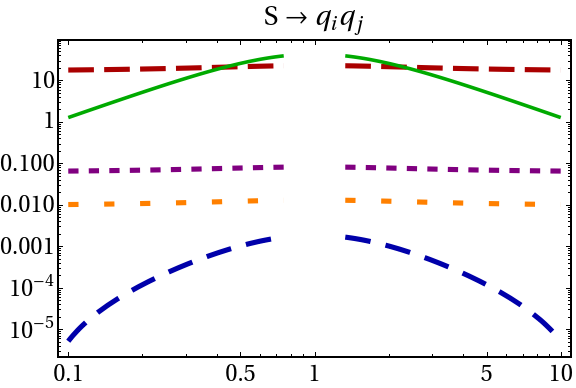
Figure 2: Log-log plot of relative branching ratios for the $S$ decay into quark-antiquark pairs, normalized by its branching ratio into a $\overline{b}b$ quark pair, as a function of $\tan\beta$, for the x2HDM-1, for $M_{S}=M_{A}=1.5\text{ TeV}$. The region for $\tan\beta$ which was excluded in Figure 1 is intentionally kept out in these plots. The relative branching ratios for $A$ are very similar.

The features shown in this section are distinctive characteristic of the x2HDMs, which can be used to falsify the models here shown.

6 Summary

In this paper, we studied some properties of a minimal extension of the SM, the 2HDM, and, in particular, focused on the study of the FCNCs of the model. We studied different variants of the 2HDM, resulting from the imposition of different symmetries on the Yukawa interactions of the model. Since these symmetries do not commute with the full gauge group of the SM Lagrangian (in practice, they are broken by the hypercharge), the imposed symmetries are effectively approximate symmetries of the theory. Taking advantage that the renormalization group equations of the 2HDM are well-known, assuming the symmetry to be a true symmetry of the Lagrangian at an energy scale $\mu$, it is possible to compute the evolution of the deviation from the symmetric situation with respect to the energy scale.

We advocate the bidoublet notation, widely popular in the context of left-right symmetric theories, applied to the context of the 2HDM. While it may seem a convoluted exercise which increases the problem’s complexity, we argue for its benefits. Namely, imposing simple symmetries on the bidoublet, we are able to recover the paradigmatic type-I and type-II 2HDM models, as well as formulate two new 2HDM variants, which until now remained unstudied.

Through this paper, our main goal was to search for models where the general arbitrariness of the FCNC couplings was reduced, following the motivation of BGL models, by relating these couplings with the quark mixing matrices. We find a class of new models, where the FCNCs are controlled by the left- and right-handed quark mixings. Due to the particular relations between the Yukawa matrices of the model, we name this new class of models the crossed 2HDM (x2HDM). In one of these such models, the x2HDM-1, we show that it is possible to impose a symmetry on the Yukawa sector such that the FCNCs are fully controlled by the left- and right-handed CKMs, as well as the ratio between the scalar doublets VEVs. We also point out that, while this symmetry is approximate in the 2HDM context, it is automatically imposed when dealing with the LRSM. As such, this model can be taken as the electroweak scale incarnation of the LRSM, given that the LRSM relies on a 2HDM structure. Following up on this intimate connection between the x2HDM-1 and the LRSM, a comprehensive flavor analysis, when paired up with the RGE study, may lead to valuable insight on the validity of some LRSMs, which we wish to explore in a future work. Furthermore, it is important to note that some of the conclusions obtained for the x2HDM-1 are equally valid or extendable to the LRSM, such as the excluded region for the Higgs-doublets’ (the bidoublet’s in the LRSM context) VEVs. We also present a second model, dubbed x2HDM-2, where the FCNC structure is further simplified, being entirely controlled by the left- and right-handed CKMs, independent of the VEV ratio. While we do not present a UV-completion for this model, we consider this model as a valuable argument for the benefits of a change of outlook (in this case, notations), to uncover new interesting possibilities.

We have also performed a phenomenological analysis of the x2HDMs, to showcase their predictive power. In the paradigm of the alignment limit, as well as assuming $M_{S}=M_{A}$, the tree-level contributions to the $\Delta F=2$ processes are simplified, but still remain. As such, the restrictive flavor data on $\Delta M_{K}$, $\Delta M_{B_{s}}$, and $\Delta M_{B_{d}}$, constrain the model. However, the same couplings are responsible not only for the neutral meson oscillations, but also for other flavor processes such as the two-body fermionic decays of the nonstandard scalars of the theory. As such, a specific example for $V_{R}$ is shown, which was obtained by requiring the compatibility of the models with $\Delta F=2$ data. It leads to specific values for the branching ratios of both $S$ and $A$ for the x2HDM-2, and a distinctive pattern of these quantities as a function of $\tan\beta$ for the x2HDM of type 1.

As a final note, hopefully, the explicit relation between the x2HDM-1 and the LRSM, together with the economical structure of the FCNCs of both x2HDMs, as well as the benefits of a change in notation for uncovering models, will lead to a renewed aesthetic motivation for the study of 2HDMs, apart from the supersymmetric embedding.

References

- [1] G. Branco, P. Ferreira, L. Lavoura, M. Rebelo, M. Sher, and J. P. Silva, Theory and phenomenology of two-Higgs-doublet models, Phys. Rept. 516 (2012) 1–102, [arXiv:1106.0034].
- [2] G. Bhattacharyya and D. Das, Scalar sector of two-Higgs-doublet models: A minireview, Pramana 87 (2016), no. 3 40, [arXiv:1507.06424].
- [3] S. L. Glashow and S. Weinberg, Natural Conservation Laws for Neutral Currents, Phys. Rev. D15 (1977) 1958.
- [4] D. Das, 2HDM without FCNC: off the beaten tracks, Eur. Phys. J. C 78 (2018), no. 8 650, [arXiv:1803.09430].
- [5] F. J. Botella, F. Cornet-Gomez, and M. Nebot, Flavor conservation in two-Higgs-doublet models, Phys. Rev. D 98 (2018), no. 3 035046, [arXiv:1803.08521].
- [6] G. C. Branco, W. Grimus, and L. Lavoura, Relating the scalar flavor changing neutral couplings to the CKM matrix, Phys. Lett. B380 (1996) 119–126, [hep-ph/9601383].
- [7] G. Bhattacharyya, D. Das, and A. Kundu, Feasibility of light scalars in a class of two-Higgs-doublet models and their decay signatures, Phys. Rev. D 89 (2014) 095029, [arXiv:1402.0364].
- [8] F. Botella, G. Branco, A. Carmona, M. Nebot, L. Pedro, and M. Rebelo, Physical Constraints on a Class of Two-Higgs Doublet Models with FCNC at tree level, JHEP 07 (2014) 078, [arXiv:1401.6147].
- [9] R. N. Mohapatra, G. Yan, and Y. Zhang, Ameliorating Higgs induced flavor constraints on TeV scale , Nucl. Phys. B 948 (2019) 114764, [arXiv:1902.08601].
- [10] G. Bhattacharyya, D. Das, P. B. Pal, and M. Rebelo, Scalar sector properties of two-Higgs-doublet models with a global U(1) symmetry, JHEP 10 (2013) 081, [arXiv:1308.4297].
- [11] D. Das and I. Saha, Search for a stable alignment limit in two-Higgs-doublet models, Phys. Rev. D 91 (2015), no. 9 095024, [arXiv:1503.02135].
- [12] P. Bhupal Dev and A. Pilaftsis, Maximally Symmetric Two Higgs Doublet Model with Natural Standard Model Alignment, JHEP 12 (2014) 024, [arXiv:1408.3405]. [Erratum: JHEP 11, 147 (2015)].
- [13] D. Das and I. Saha, Alignment limit in three Higgs-doublet models, Phys. Rev. D 100 (2019), no. 3 035021, [arXiv:1904.03970].
- [14] F. J. Botella, G. C. Branco, and M. N. Rebelo, Minimal Flavour Violation and Multi-Higgs Models, Phys. Lett. B687 (2010) 194–200, [arXiv:0911.1753].
- [15] R. Mohapatra and J. C. Pati, A Natural Left-Right Symmetry, Phys. Rev. D 11 (1975) 2558.
- [16] R. N. Mohapatra and J. C. Pati, Left-Right Gauge Symmetry and an Isoconjugate Model of CP Violation, Phys. Rev. D 11 (1975) 566–571.
- [17] G. Senjanović and R. N. Mohapatra, Exact Left-Right Symmetry and Spontaneous Violation of Parity, Phys. Rev. D 12 (1975) 1502.
- [18] N. G. Deshpande, J. F. Gunion, B. Kayser, and F. I. Olness, Left-right symmetric electroweak models with triplet Higgs, Phys. Rev. D44 (1991) 837–858.
- [19] D. Atwood, L. Reina, and A. Soni, Phenomenology of two Higgs doublet models with flavor changing neutral currents, Phys. Rev. D 55 (1997) 3156–3176, [hep-ph/9609279].
- [20] M. Nebot and J. P. Silva, Self-cancellation of a scalar in neutral meson mixing and implications for the LHC, Phys. Rev. D 92 (2015), no. 8 085010, [arXiv:1507.07941].
- [21] L. Wolfenstein, Parametrization of the Kobayashi-Maskawa Matrix, Phys. Rev. Lett. 51 (1983) 1945.