Marginally Trapped Surfaces in Spherical Gravitational Collapse

Abstract

This paper deals with a detail study of gravitational collapse of dust and viscous fluids under the assumptions of spherical symmetry. Our main goal is to closely analyze the horizons which arise during this gravitational phenomenon. To this end, we examine the formation and evolution of trapped surfaces in these spacetimes, with special attention to trapped regions and cylinders foliated by marginally trapped surfaces. The time evolution of trapped surfaces, collapsing shell as well as the event horizon are identified analytically as well as numerically. Using different density profiles of matter, we analyze, how the nature of the marginally trapped surfaces modify as we change the energy momentum tensor. These studies reveal that depending on the mass function and the mass profile, it is possible to envisage situations where dynamical horizons, timelike tubes or isolated horizons may arise.

1 Introduction

The study of collapse of a self- gravitating isolated system is of great importance in general relativity. Not only this problem is of physical importance, particularly in understanding the formation of black holes and large scale structures in the universe, but also raises fundamental queries related to formation of horizons, spacetime singularities and the cosmic censorship conjecture [1, 2, 3, 4, 5, 6]. The study of gravitational collapse, began with the independent work of Dutt [7] and Oppenheimer and Snyder [8] (OSD). Although the OSD model was limited to collapse of a dust cloud of homogeneous density, it provided important clues to the nature and mode of formation of spacetime singularities out of a self gravitating matter system. In particular, it shows that within a finite proper time, the spherical ball of matter collapses to a proper radius smaller than its Schwarzschild radius. Eventually, the entire self gravitating matter collapses to a point of infinite density and curvature, usually called a spacetime singularity. Furthermore, once the matter has crossed the Schwarzschild horizon, no light is able to escape to observers at asymptotic infinity and hence the singularity remains hidden to the outside world [1, 2, 3]. This is the well known scenario of black hole formation. Though the OSD model is simple, the mathematical structure may be used to understand more complicated and real life examples of collapse of massive astrophysical systems. It has been argued, quite rightly, that the gravitational collapse of real stars may not follow the idealised dynamical situation as described in the OSD model. The collapsing cloud of matter may be inhomogeneous, have internal pressure, and even possess properties generic to fluids, like viscosity and pressure anisotropies. For example, the well known Lemaitre- Tolman- Bondi (LTB) model of collapse describes the inhomogeneous, pressureless gravitational collapse [9, 10, 11]. To understand these large variety of situations, general formalism to study dynamical evolution of collapse has been developed. In this method, under various regularity and energy conditions, the initial data is provided in terms of the initial density, pressures, and velocity profiles, and the dynamical evolution is studied using the Einstein equations [4, 12, 13]. It has been argued that under a large number of fairly regular initial data, both black holes and naked singularities may evolve (a nice review is given in [4, 14]. The OSD model for example, shows that once the collapse starts it eventually reaches an epoch (that of horizon formation at the Schwarzschild radius) when no light emitted from its surface can escape to faraway observers, and hence leading to a black hole. A naked singularity is not covered by a horizon but is also interesting since an observer at infinity may communicate with it. Naked singularities have a large literature and are discussed in [15, 16, 17, 18, 19, 20, 21, 22, 23, 24, 25, 26, 27, 28, 29, 30, 31, 32, 33, 34, 35]. The singularity is said to be naked locally (or globally) if a non- spacelike geodesic emanates from it to reach the neighbourhood (or asymptotic infinity). Indeed, in many instances, regular initial data in inhomogeneous, pressureless collapse develop into strong curvature naked singularities. Another class of singularity which remains visible to observers at infinity is called the shell- crossing singularity [36]. These indicate breakdown of the coordinate system and hence, are not genuine spacetime singularities. Shell- crossing singularities are gravitationally weak [37], but care must be taken to avoid them.

It is now well known that any general relativistic collapse of isolated gravitating matter satisfying regular initial data always results in a spacetime singularity in the form of geodesic incompleteness if a trapped surface forms, and certain reasonable energy conditions on matter and causal structure of the spacetime holds [1, 2]. Additionally, the censorship conjecture, rules that the gravitational collapse of matter fields under generic conditions result in the formation of spacetime singularity which shall remain clothed from the outside world by a horizon. The statement of this conjecture are encoded in the weak as well as the strong versions of the conjecture and has been shown to hold true for simple systems (see [38, 39] for review). So, if the censorship conjecture is assumed correct, the collapse must be followed by an horizon. The most natural description of horizons is the Event Horizon (EH). However, one fundamental objection against the event horizon formalism is that it is too global. Indeed, for this definition to work, one must have access to the global development of the spacetime, which may not be possible in all cases. For example, in a numerical study of a black hole spacetime, the location of the EH is only possible if the entire evolution of the spacetime has been obtained, although the numerical evolution itself requires the horizon to be located on each time slice. Such inconsistencies have led to many local definitions of horizon (a detailed overview is in [40, 41, 42, 43]). Out of these, the marginally trapped surface (MTS) is quite useful. This is a closed $2$- dimensional surface, such that the expansion scalar of the outgoing null normal vanishes $\theta_{(\ell)}=0$, while that of the ingoing null normal is negative $\theta_{(n)}<0$. This definition has proved to be quite useful, since the Marginally Trapped Tube (MTT) formed out of stacking MTSs does not have any signature associated to it. Indeed, a null MTT is an isolated horizon (IH) and hence describes a black hole horizon in equilibrium. When the MTT is spacelike, it is a dynamical horizon (DH), and describes a growing black hole. If the MTT has a timelike signature, it is called a timelike tube, through which matter may cross in either directions. Thus MTTs provide an unified framework to study time evolution of black holes through different phases. The nature of MTTs and their behavior due to some dust models of collapse like the LTB have been studied in [44], and very recently in [45, 46]. However, our study focuses on both the analytical and numerical aspect of the evolution of the MTT. In particular for the homogeneous dust models, we identify the beginning of formation of MTT, and trace it until it stops evolving, eventually matching with the isolated horizon. Furthermore, we also include a detail study of MTTs forming due to gravitational collapse of more general energy- momentum tensors including viscous effects.

The main motive of this paper is to discuss methods which will be useful to, (i) construct spherically symmetric models of spacetime for fluids with general energy- momentum tensors, (ii) study the collapse end state with special emphasis on the formation of horizons, and in particular, track the marginally trapped tubes in each of the cases, and (iii) identify, for the mass profiles considered here, the regions of the parameter space where the MTT evolves as a DH (when matter fall through it), where it might be timelike, and when it does become an IH. In each of the examples, the exterior geometry will be assumed to be the Schwarzschild spacetime. The study will include OSD/LTB models and the ones obtained by dropping the assumptions of homogeneity and local anisotropy in the fluid energy- momentum tensor. Interest in these generalities in the equation of state stems from the fact that there is a growing attention in understanding the phenomenon of collapse of astrophysical systems with different equation of states and energy-momentum tensors [47, 48, 49, 50, 51]. As particular examples, the energy momentum tensors we consider below shall include locally anisotropic fluids, without heat flux, but with shear and bulk viscosity. Local anisotropy in the interior fluid have been argued to arise due to various causes including viscosity or local anisotropic velocity distributions. Such anisotropies would naturally break the conditions of fluid isotropy and hence, in presence of viscosity, radial and transverse pressures must be different (in section $5$, we present a proof). Furthermore, it has been shown that shearfree condition, particularly in the presence of anisotropy of the pressure and dissipation, leads to instability. These kind of inhomogeneities and anisotropies in the matter fields are expected to occur quite naturally in the astrophysical systems, particularly during the gravitational collapse, and are expected to play a major role in deciding the spacetime structure. In particular, it has been argued that shear may be responsible for the violation the cosmic censorship leading to a naked singularity in the spacetime [4]. Thus, it is important that a detail study into these aspects must be made and indeed similar kind of models have received attention on the past (see for example [52, 53]). However, most of the metric configurations are either static or with restricted time dependence. On the other hand, we expect that, in presence of heat flux, viscosity or pressure terms, the interior spacetime would be highly dynamical and respond to any fluctuations in the energy momentum tensor. To incorporate these attributes, in this paper, we relax the assumptions of staticity and generalise these geometries to include time dependence, making these models closer to realistic dynamical systems. More specifically, including anisotropic pressure and the shear and bulk viscosity terms, we construct explicitly dynamical metric functions (we must however ensure that the viscosity effects are not huge to destroy the spherical symmetry of the spacetime and in the examples, we have chosen the coefficients in this manner). These metric functions are then used to study the end state of the spherically symmetric collapse, leading to a central singularity, and trapped surface formation.

The paper is arranged as follows. In the section 2, we set up the definitions of the different class of horizons which we shall use in this paper. We discuss the inadequacies of the EH and the advantages of the MTT formalism. In section 3, we set- up our conventions and the mathematical framework for the Einstein equations as an initial value framework. We also spell out the boundary conditions, along with those required for smooth gravitational collapse. For example, we ensure that there is no shell crossing singularities and that the initial spacelike surface does not have any trapped region. The section 4 discusses the pressureless collapse models including the OSD and the LTB models. While these models are quite well known (the marginally bounded OSD models are described in [54, 55] using the Painleve- Gullstrand coordinates, and in [3, 49] using the standard coordinates), we give detailed analytical calculations, along with the boundary conditions to show how the collapse scenario proceeds. In particular, we present analytical formula for (i) collapse of the shells, (ii) time development of event horizon, and (iii) time development of the marginally trapped tube (or sometimes called the apparent horizon). In several of the collapse scenarios, like the OSD models, the study of formation and evolution of MTT can be carried out exactly through analytical methods. In section 4, the behavior of MTT for each of the three subcases of the OSD model: marginally bounded, bounded and unbounded collapse respectively are given. The analytical results, followed by detail numerical models corroborate exactly. For inhomogenous dust collapse models like LTB, the simple mass profiles may be understood through analytical tools, but for realistic mass profiles, we rely on numerical methods. We consider several density profiles and, in each case, determine the evolution of MTT. Section 5 studies models of spacetimes due to viscous fluids. We begin with some generic properties these spacetimes must be endowed with. We show that if the fluid has shear and bulk viscosity, as well as pressure anisotropy, then generically the spacetime will not admit isotropy, conformal flatness or spatially uniform expansion scalar. We also take various cases to show that the effects of viscosity (again keeping the non- spherical effects small) on the formation of the MTT. In particular, we show that the viscous effects may delay or advance the formation of MTT depending on the coefficients of viscosity. These effects of viscosity are exemplified through various choices of parameters and mass functions. We conclude in section 6.

2 Horizons and Marginally Trapped Tubes

In the standard description, a black hole horizon is a future event horizon (EH), which, in an asymptotically flat spacetime, is defined as boundary of the past of future null infinity, $\partial[J^{-}(\mathscr{I}^{+})]$ [1, 2]. This definition is powerful since it is an invariant construct based only on geometrical arguments and asymptotic structure of spacetime. However, this definition is difficult to implement in many practical situations, although the situation simplifies for equilibrium situations (see [41, 42] for a detailed review). In equilibrium, the spacetime is stationary and admits Killing vector fields one of which may be identified with the time translation generator at asymptotic infinity. Naturally, these Killing vector fields are tangential to the EH. Thus, in stationary spacetimes, the EH may be described as a Killing Horizon, generated by a null Killing vector field. A clear example is provided by the spherically symmetric Schwarzschild spacetime. This is a stationary spacetime which admits four global Killing vector fields, three of which are spacelike, generating the $2$- sphere isometries and a time translation generator $(\partial/\partial t)$. This timelike Killing vector becomes null generator on the horizon $R=2M$. Note however, that if a spacetime is not in equilibrium (for example, the Vaidya spacetime), Killing Horizon cannot be constructed and hence, one has to resort to the abovementioned definition of EH to locate horizon for this spacetime.

However, the EH, as a definition, is far from useful even in dynamical spacetimes. The notion is global since it requires knowledge of the entire future evolution of the spacetime (which may include a black hole region as well), to locate the future null infinity and hence, ascertain the existence of a black hole horizon. Quite simply, the definition does not work in practical situations, like those studied in numerical relativity where, one cannot even evolve the spacetime if the horizon is not located on a given time slice (a comprehensive discussion on these problems, and the need for quasilocal horizons in numerical relativity is discussed in [40, 41, 42, 43]). A vivid description of the difficulties associated with this definition and its teleological nature is captured through the Hartle- Hawking formula [56]. This formula shows that the area of an event horizon of a dynamical black hole at the final time $t_{f}$ (when the matter has stopped falling) is dependent also on the beheviour of geometrical quantities at times $t>t_{f}$. More precisely, area of any dynamically evolved EH may only be determined if the full global evolution of the spacetime along with precise knowledge of values of geometrical fields for all future times is known. A further critique of EH was given in [57], where it was argued that simple local modifications of the black hole region (which may be quantum mechanical in nature, and hence beyond the scope of classical GR) may get rid of the formulation of EH. These arguments underscore the need for a quasilocal description of black hole horizons which however, must capture all the essential physics details EH has given us.

The local notion of horizons are based on the definition of trapped surfaces which, loosely speaking, characterize regions of spacetime from which light rays cannot escape to infinity [5]. In these regions, null rays orthogonal to closed $2$- surfaces have negative expansion. More precisely, if $\ell^{a}$ and $n^{a}$ are respectively the outgoing and the ingoing null vectors orthogonal to a $2$- sphere, then this $2$-surface is called trapped if their respective expansions, $\theta_{(\ell)}$ and $\theta_{(n)}$ are both negative. In general, the $2$-sphere is called untrapped, trapped or marginally trapped depending on whether $\theta_{(\ell)}$ is greater, less or equal to zero respectively. Using these marginally trapped surfaces, one may formulate a definition of horizon. The notion of apparent horizon is one such local description which found several applications in local black hole dynamics. However, since apparent horizon depends on the choice of foliation of spacetime by spacelike hypersurfaces, several examples exist where the apparent horizon has been difficult to locate. Even in simple cases like the Schwarzschild spacetime, where the existence of horizon is unambiguous, the apparent horizon may be difficult to locate [58]. As a remedy, a quasilocal formulation called Trapping Horizon (TH) were introduced in [59]. They are defined as follows: A trapping horizon, denoted here by $\Delta_{T}$ is a $4$-dimensional spacetime, foliated by $S^{2}$ such that the expansions of the null normals $\ell^{a}$ (outgoing) and $n^{a}$ (ingoing) orthogonal to the foliations have expansions $\theta_{(\ell)}|_{\Delta_{T}}=0$, $\theta_{(n)}|_{\Delta_{T}}\neq 0$ such that $\pounds_{n}\theta_{(\ell)}|_{\Delta_{T}}\neq 0$. If $\theta_{(n)}|_{\Delta_{T}}<0$, the horizon is termed future, whereas it is past otherwise. Furthermore, a horizon is called an outer trapping horizon if $\pounds_{n}\theta_{(\ell)}|_{\Delta_{T}}<0$ , whereas, it is termed inner if $\pounds_{n}\theta_{(\ell)}|_{\Delta_{T}}>0$. In fact, Future Outer Trapping horizons (FOTH) have found important applications in the proof of laws of black hole mechanics [59] as well as in developing local formulations of Hawking radiation mechanism [60].

The formulations of Isolated Horizons (IH) [61, 62] and Dynamical Horizons (DH) [63, 64], which are closely related to THs, have led to crucial insights towards understanding classical and quantum behavior of black hole horizons. They have also found important applications in the development of numerical methods used to study horizon formation, their mergers and gravitational waves. Indeed, the IH formalism which describes the equilibrium states of black hole, have been used to develop Hamiltonian techniques for black hole mechanics. More specifically, the space of solutions of Einstein’s theory, with IH as an inner boundary, admits a phase- space formulations along with a well defined symplectic structure and surprisingly, the first law of black hole mechanics turns out to be the necessary and sufficient condition for a consistent Hamiltonian evolution in the phase- space [61, 62]. Additionally, this framework also provides the boundary symplectic structure which allows identification of the boundary quantum states responsible for black hole entropy [65]. The DH plays a crucial role in understanding smooth dynamical evolution of black hole horizons. The first law (in terms of fluxes) for such a dynamical evolution provides a useful theoretical framework to model black holes evolution [63, 64]. Further developments in these directions have been in the development of quasispherical and perturbative approximations of the IH and the DH formalisms. In the dynamical set-up it has been possible to construct a class of evolving horizons, called the Conformal Killing Horizons (CKH) which are null, but admit a well defined phase- space description in the first order connection- tetrad variables. Indeed, it has also been possible, even in this dynamical framework, to derive a differential version of the first law of black hole mechanics, arising due to influx of (scalar) matter terms [66, 67].

A unified quasilocal framework to describe horizons, called Marginally Trapped Tube (MTT) was developed in [69]. Let $(\mathcal{M},g_{ab})$ be a $4$- dimensional spacetime with signature $(-,+,+,+)$. We shall use the Newmann- Penrose null basis $(\ell^{a},n^{a},m^{a},\bar{m}^{a})$, where $\ell\cdot n=-1$, $m\cdot\bar{m}=1$, while all other dot products vanish. Let $\Delta$ be a hypersurface in $\mathcal{M}$. In the following, we shall not restrict the signature of $\Delta$ and hence, it may be spacelike, timelike or even null. Let us assume that $\Delta$ is topologically $S^{2}\times\mathbb{R}$. Let $\ell^{a}$ and $n^{a}$ are respectively the outgoing and the ingoing vector fields orthogonal to the $2$- sphere cross-sections of $\Delta$. If $t^{a}$ is a vector field tangential to $\Delta$ and normal to foliations, $t^{a}$ may be written in terms of the ingoing and the outgoing null vector fields as: $t^{a}=\ell^{a}-Cn^{a}$ (the sign of $C$ is in accordance with the conventions in [44]). Since $t\cdot t=2C$, the constant $C$ determines the signature of the MTT.

The hypersurface $\Delta$ will be called a Marginally Trapped Tube (MTT) if the following conditions hold true on $\Delta$:

1. $\theta_{(\ell)}=0$,

2. $\theta_{(n)}<0$.

Several comments are in order regarding these boundary conditions. First, MTT may be viewed as a unified formalism to describe black hole horizons since $\Delta$ has no restriction on its signature. When MTT is null it describes black holes in equilibrium (an IH), a growing black holes (a DH) when it is spacelike, or simply a timelike membrane (when $\Delta$ is timelike), allowing matter to cross it. The advantage of the MTT formalism is that instead of looking at the evolution of horizons through various phases: dynamical horizons, isolated horizons, and timelike membranes (each phase multiple number of times), one may view horizons as the time evolution of a single MTT. Secondly, MTT admits much weaker set of conditions than either the IH or the DH formalism. For example, no restiction on $\pounds_{n}\theta_{(\ell)}$ is assumed. If $\pounds_{n}\theta_{(\ell)}<0$, the MTT shall be called a FOTH. Thirdly, MTTs are foliated by marginally trapped $2$- spheres. Since $t^{a}$ is orthogonal to the foliations and tangential to $\Delta$, it generates a foliation preserving flow so that the following condition holds on $\Delta$

$$\pounds_{t}\,\theta_{(\ell)}\triangleq 0.$$ (1)

Fourth, the constant $C$ also measures the evolution of MTT. To see this, note that if $m^{a}$ and $\bar{m}^{a}$ are tangential to the $2$- sphere cross-sections, the area element is given by ${}^{2}\mathbf{\epsilon}=im\wedge\bar{m}$. Under the flow generated by $t^{a}$, the area element of MTT evolves as:

$$\pounds_{t}\,{}^{2}\mathbf{\epsilon}=-C\,\theta_{(n)}\,{}^{2}\mathbf{\epsilon}$$ (2)

Naturally, the timelike MTT (for which $C<0$) contracts, null MTT ($C=0$) does not grow, whereas spacelike MTT (for which $C>0$) expands. Furthermore note that no condition on the energy- momentum tensor is assumed on $\Delta$. The Einstein equation $G_{ab}\equiv R_{ab}-(1/2)R\,g_{ab}=T_{ab}$shall be assumed to hold on $\Delta$.

Several conclusions follow from these conditions, detail calculations of various equations are given in [68]. From (1), the constant $C$ is determined by the condition

$$C=\frac{\pounds_{\ell}\,\theta_{(\ell)}}{\pounds_{n}\,\theta_{(\ell)}}.$$ (3)

To determine the value of the constant $C$, one uses the Newmann- Penrose equations for the MTT. Using $\theta_{(\ell)}=0$ and the Einstein equation $G_{ab}=T_{ab}$, we get the following two equations:

$$\pounds_{\ell}\,\theta_{(\ell)} = -T_{ab}\ell^{a}\ell^{b},$$ (4)

$$\pounds_{n}\,\theta_{(\ell)} = -(\mathcal{R}/2)+T_{ab}\ell^{a}n^{b}.$$ (5)

Here, $\mathcal{R}$ is the scalar curvature of the round $2$- sphere and may be rewritten as $\mathcal{R}=(8\pi/\mathcal{A})$, where $\mathcal{A}$ is area of $2$- sphere. These equations imply that the constant $C$ which determines the nature of the MTT is given by:

$$C=\frac{T_{ab}\ell^{a}\ell^{b}}{(4\pi/\mathcal{A})-T_{ab}\ell^{a}n^{b}}$$ (6)

It follows from the discussion above that the signature of $\Delta$, determined by $C$, is a quantity of utmost importance since it decides the nature and stability of horizon [70, 71]. From the above equation (6), this value is controlled by the energy- momentum tensor and area of the marginally trapped surfaces. In the following, we shall use several energy-momentum tensors, including dust models and viscous fluids, and evaluate $C$ in each case. However, as we shall see below, the form of $T_{ab}$ is not the only criteria deciding the signature of MTT, the mass profile and the equations of collapse are also important factors. Given these complicated constraints, the generic behavior of MTT is not known for arbitrary black hole evolution. Consider for example, Vaidya- type black holes evolving under matter fields satisfying dominant energy conditions, the evolution of the MTT is described by the equation $R=2m(v)$, where $v$ is the advanced Eddington- Finkelstein coordinate. In this case, the MTT is spacelike (more precisely, it is a DH) if $\dot{m}(v)>0$, where dot indicates derivative with respect to the advanced time coordinate [63, 64, 73]. However, this conclusion does not hold true for any arbitrary collapse scenarios. Indeed, even for simple situations like the OSD models of homogeneous dust collapse, a timelike MTT (or a timelike membrane) appears just as the matter cloud reaches the Schwarzschild radius. This timelike membrane, together with the matter cloud, eventually collapses into the singularity at exactly the same time. Examples of trapped surfaces are also discussed in [43, 44, 54, 72, 74, 75, 76, 77, 78, 79, 80, 81]. In more realistic LTB inhomogenous collpase models, the matter cloud and the MTT behave drastically differently: the cloud shells reach singularity at different times and the MTT is not purely timelike. For large number of cases, in which the matter profile is smooth, the MTT begins as a spacelike hypersurface from the center of the cloud and asymptotes to the null event horizons as infall of matter is discontinued. For mass profiles with more complicated functional forms, time evolution of MTT shows strange behavior: for example, turning timelike from being spacelike through an intermediate (expanding) null regions. These details are studied with large number of examples as well in the following sections.

3 Spherical Symmetric Collapse formalism

Let us consider a general spherically symmetric ball of fluid with the line element

$$ds^{2}=-e^{2\alpha(r,t)}dt^{2}+e^{2\beta(r,t)}dr^{2}+R(r,t)^{2}d\theta^{2}+R(r,t)^{2}\sin^{2}{\theta}\,d\phi^{2},$$ (7)

where $\alpha(r,t)$ and $\beta(r,t)$ are spacetime dependent functions, $\theta$ and $\phi$ are the angular variables on the sphere and $R(r,t)$ is the radius of the sphere. This is the standard frame, where the fluid velocity is $u^{a}=u\,(\partial/\partial t)^{a}$. This frame allows for a simpler integration of the Einstein equation and the Bianchi identities. The tetrad basis is suitable for obtaining the Einstein equations. The set of tetrad one forms obtained from the metric are as follows:

$$e^{0}=e^{\alpha(r,t)}\,dt,~{}~{}e^{1}=e^{\beta(r,t)}\,dr,~{}~{}e^{3}=R\,d\theta,~{}~{}e^{4}=R\sin\theta\,d\phi.$$ (8)

The Riemannian spin- connection may be obtained from the torsion- free condition, $de^{I}+\omega^{I}_{J}\wedge e^{J}=0$, where $I,J$ are the internal flat basis, with $I,J,K,\dots=0,1,2,3$. The spin- connections are obtained to be:

$$\omega^{0}{}_{1}=\left(\alpha^{\prime}\,e^{-\beta}\right)\,e^{0}+\left(\beta^{\prime}\,e^{-\alpha}\right)\,e^{1},~{}~{}~{}~{} \omega^{0}{}_{2}=(\dot{R}/R)\,e^{-\alpha}\,e^{2},$$

$$\omega^{1}{}_{2}=-(R^{\prime}/R)\,e^{-\beta}\,e^{2},~{}~{}~{}~{} \omega^{2}{}_{3}=-(\cot\theta/R)\,e^{3}.$$ (9)

The curvature two form, $\Omega_{IJ}$, are given by, $\Omega_{IJ}=d\omega_{IJ}+\omega_{IK}\wedge\omega^{K}{}_{J}$ and the non-zero ones are ($i,j=2,3$):

$$\Omega^{0}{}_{1} = \left[\left\{e^{-\alpha}\,(e^{\beta})_{,t}\right\}_{,t}-\left\{e^{-\beta}\,(e^{\alpha})_{,r}\right\}_{,r}\right]e^{-(\alpha+\beta)}\,\,e^{0}\wedge e^{1},$$

$$\Omega^{0}{}_{i} = \left[\frac{e^{-\alpha}}{R}\left\{(R)_{,t}\,\,e^{-\alpha}\right\}_{,t}-\frac{R_{,r}}{R}(e^{\alpha})_{,r}\,\,e^{-(\alpha+2\beta)}\right]\,e^{0}\wedge e^{i}$$

$$~{}~{}~{}~{}~{}~{}~{}~{}~{}~{}~{}~{}~{}~{}+\left[\frac{e^{-\beta}}{R}\left\{(R)_{,t}\,\,e^{-\alpha}\right\}_{,r}-\frac{R_{,r}}{R}(e^{\beta})_{,t}\,\,e^{-(\alpha+2\beta)}\right]\,e^{1}\wedge e^{i}$$

$$\Omega^{1}{}_{i} = \left[-\frac{e^{-\alpha}}{R}\left\{(R)_{,r}\,e^{-\beta}\right\}_{,t}-\frac{R_{,t}}{R}(e^{\alpha})_{,r}\,\,e^{-(2\alpha+\beta)}\right]\,e^{0}\wedge e^{i}$$

$$~{}~{}~{}~{}~{}~{}~{}~{}~{}~{}~{}~{}~{}~{}+\left[-\frac{e^{-\beta}}{R}\left\{(R)_{,r}\,e^{-\beta}\right\}_{,r}-\frac{R_{,t}}{R}(e^{\beta})_{,t}\,\,e^{-(2\alpha+\beta)}\right]\,e^{1}\wedge e^{i}$$

$$\Omega^{2}{}_{3} = \left[\left(\frac{R_{,t}}{e^{\alpha}R}\right)^{2}-\left(\frac{R_{,r}}{e^{\beta}R}\right)^{2}\right]\,e^{2}\wedge e^{3}+(1/R^{2})\,e^{2}\wedge e^{3}.$$ (10)

The components of the curvature two torms may be extracted by using $\Omega_{IJ}=(1/2)\,\Omega_{IJKL}\,e^{K}\wedge e^{L}$ and the Ricci tensor components are given by $R_{IJ}=\Omega^{K}{}_{IKL}$. The Einstein tensor in the orthornormal frame is easily obtained by using the equation $G_{IJ}=R_{IJ}-(1/2)\eta_{IJ}R$, with $R=\eta_{IJ}R^{IJ}$. In this tetrad basis, the four velocity is given by $u^{I}=(1,\vec{0}\,)$. Using the standard frame transformation rules, $e^{I}{}_{a}\,u^{a}=u^{I}$, the velocity vector in the coordinate basis becomes, $u^{a}=e^{-\alpha}\,(\partial/\partial t)^{a}$. From now on, we shall use the coordinate basis for our explicit calculations.

We envisage the solutions of the Einstein equation for the energy- momentum tensor of the spherical ball given by the following form:

$$T_{ab}=(p_{t}+\rho)\,u_{a}u_{b}+p_{t}\,g_{ab}+(p_{r}-p_{t})\,X_{a}\,X_{b}-2\eta\,\sigma_{ab}-\zeta\theta h_{ab},$$ (11)

where $\eta$ and $\zeta$ are the coefficients of shear and bulk viscosity, $X^{a}$ is a unit space-like vector tangential to the spacelike section orthogonal to $u^{a}$ respectively satisfying $X_{a}X^{a}=1$. The quantities $\sigma_{ab},\theta$, and $h_{ab}$ are shear, expansion and projection tensor and, $\rho$, $p_{t}$ and $p_{r}$ are the energy density and tangential and radial components of pressure respectively. The expressions for these quantities are

$$\theta = \nabla_{a}u^{a},~{}~{}~{}~{}h^{a}{}_{b}=(\delta^{a}{}_{b}+u^{a}u_{b}\,)$$ (12)

$$\sigma^{ab} = \frac{1}{2}\left(h^{ac}\,\nabla_{c}\,u^{b}+h^{bc}\,\nabla_{c}\,u^{a}\right)-\frac{1}{3}\theta P^{ab},$$ (13)

$$X^{a} = e^{-\beta(r,t)}\,(\partial/\partial r)^{a}$$ (14)

Their values for this metric is easily determined to be:

$$\theta=e^{-\alpha}(\dot{\beta}+2\dot{R}/R),$$ (15)

$$h_{ab}=e^{2\beta(r,t)}dr^{2}+R(r,t)^{2}d\theta^{2}+R(r,t)^{2}\sin^{2}{\theta}\,d\phi^{2},$$ (16)

$$\sigma^{1}{}_{1}=(2/3)\,(\dot{\beta}-\dot{R}/{R})e^{-\alpha},$$ (17)

$$\sigma^{2}{}_{2}=\sigma^{3}{}_{3}=(-1/3)\,(\dot{\beta}-\dot{R}/{R})e^{-\alpha}.$$ (18)

Let us define a shear scalar, $\bar{\sigma}^{2}=\sigma_{ab}\,\sigma^{ab}$ and from the above expressions, we get

$$\bar{\sigma}^{2}=(2/3)e^{-2\alpha}(\dot{\beta}-\dot{R}/{R})^{2}.$$ (19)

In many cases, for simplification, we shall get rid of the $(2/3)$ factor and redefine $\sigma=e^{-\alpha}(\dot{\beta}-\dot{R}/{R})$. The non- zero components of energy-momentum tensor are given by the following quantities:

$$T^{0}{}_{0}=-\rho,\,\,~{}~{}T^{1}{}_{1}=p_{r}-\frac{4}{3}\eta\sigma-\theta\zeta,\,\,~{}~{}T^{2}{}_{2}=T^{3}{}_{3}=p_{t}+\frac{2}{3}\eta\sigma-\theta\zeta.$$ (20)

Let us now have a look at the Bianchi identities, $\nabla_{a}\,T^{ab}=0$. This gives the following two equations. The first is the $t$- equation

$$\dot{\rho}e^{-\alpha}+(\rho+p_{t})\theta+(p_{r}-p_{t})\dot{\beta}e^{-\alpha}-(4/3)\,\eta\sigma^{2}-\zeta\theta^{2}=0,$$ (21)

and the second is the $r$- equation given by the following equation,

$$(p_{t}-\zeta\theta)^{\prime}+\alpha^{\prime}(\rho+p_{t}-\zeta\theta)-(4/3)\,\eta\sigma^{\prime}-(4/3)\eta\sigma\,(\alpha^{\prime}+3R^{\prime}/R)$$

$$~{}~{}~{}~{}~{}~{}~{}~{}~{}~{}~{}~{}~{}~{}~{}~{}~{}~{}~{}~{}~{}~{}~{}~{}~{}~{}~{}~{}~{}~{}~{}~{}~{}~{}+(p_{r}-p_{t})^{\prime}+(\alpha^{\prime}+2R^{\prime}/R)(p_{r}-p_{t})=0.$$ (22)

A simple rearrangement of equation $\eqref{t-Bianchi}$ leads to the following expression for the $\dot{\beta}$:

$$\dot{\beta}=-\frac{\dot{\rho}}{\rho+p_{r}-(4/3)\,\eta\sigma}-\frac{2\dot{R}}{R}\,\frac{\rho+p_{t}+(2/3)\eta\sigma-\zeta\theta}{\rho+p_{r}-(4/3)\eta\sigma-\zeta\theta}\,.$$ (23)

On rearranging, the equation (3) similarly leads to the following equation:

$$\alpha^{\prime}=\frac{2R^{\prime}}{R}\frac{p_{t}-p_{r}+2\eta\sigma}{\rho+p_{r}-(4/3)\eta\sigma-\zeta\theta}-\frac{(p_{r}-4/3\,\eta\sigma-\zeta\theta)^{\prime}}{\rho+p_{r}-(4/3)\eta\sigma-\zeta\theta}\,\,.$$ (24)

Let us now consider the $R_{01}$ component of the Einstein equation, which is given by:

$$\alpha^{\prime}\dot{R}+\dot{\beta}R^{\prime}-{\dot{R}}^{\prime}=0.$$ (25)

Using the expressions of $\alpha^{\prime}$ from equation (24) and $\dot{\beta}$ from (23) in the abovementioned equation (25) and multiplying by $R^{2}$, we get that:

$$[(p_{r}-4/3\,\eta\sigma-\zeta\theta)\,R^{2}\,\dot{R}\,]_{,r}+[\rho R^{2}R^{\prime}]_{,t}=0$$ (26)

It is natural to interpret the exact differential to construct a function $F(r,t)$, such that

$$F^{\prime}\propto\rho\,R^{2}R^{\prime},$$ (27)

$$\dot{F}\propto-(p_{r}-4/3\,\eta\sigma-\zeta\theta)\,R^{2}\,\dot{R},$$ (28)

with the same proportionality factors. We shall call this function $F(r,t)$ as the mass function. To detremine the exact form of the mass function $F$, let us look at the Einstein equations $G_{00}$ and $G_{11}$ respectively. They are given by the following two equations:

$$\left(\frac{2R^{\prime}\beta^{\prime}}{R}-\frac{2R^{\prime\prime}}{R}-\frac{R^{\prime 2}}{R^{2}}\right)\,e^{-2\beta}+\left(\frac{2\dot{R}\dot{\beta}}{R}+\frac{\dot{R}^{2}}{R^{2}}\right)\,e^{-2\alpha}+\frac{1}{R^{2}}=\rho,$$ (29)

$$\left(\frac{2\alpha^{\prime}{R}^{\prime}}{R}+\frac{{R^{\prime}}^{2}}{R^{2}}\right)e^{-2\beta}+\left(\frac{2\dot{\alpha}\dot{R}}{R}-\frac{\dot{R}^{2}}{R^{2}}-\frac{2\ddot{R}}{R}\right)e^{-2\alpha}-\frac{1}{R^{2}}=p_{r}-\frac{4}{3}\eta\sigma-\zeta\theta.$$ (30)

Using the $G_{01}=R_{01}$ equation, and multiplying $G_{00}$ by $RR^{\prime}$ and the $G_{11}$ equation by $R\dot{R}$, the equations above reduce to:

$$\left[R(1+\dot{R}^{2}e^{-2\alpha}-R^{\prime 2}e^{-2\beta})\right]_{,\,r}=\rho R^{2}R^{\prime},$$

$$\left[R(1+\dot{R}^{2}e^{-2\alpha}-R^{\prime 2}e^{-2\beta})\right]_{,\,t}=-(p_{r}-\frac{4}{3}\eta\sigma-\zeta\theta)R^{2}\dot{R}.$$ (31)

So, comparing (27) and (3), the mass function is given by the following

$$F(r,t)=R(1+\dot{R}^{2}e^{-2\alpha}-R^{\prime 2}e^{-2\beta}).$$ (32)

This is the same equation as the Misner- Sharp mass function for the spherical symmetry. Let us now collect the equations for our problem of gravitational collapse of viscous fluids. Defining the two functions, $H=e^{-2\alpha(r,t)}\dot{R}^{2}$ and $G=e^{-2\beta(r,t)}R^{\prime 2}$, the equations reduce to:

$$\rho=\frac{F^{\prime}}{R^{2}R^{\prime}}\,\,,$$ (33)

$${p}_{r}=-\frac{\dot{F}}{R^{2}\dot{R}}+\frac{4}{3}\eta\sigma+\zeta\theta\,\,,$$ (34)

$$\alpha^{\prime}=\frac{2R^{\prime}}{R}\frac{p_{t}-p_{r}+2\eta\sigma}{\rho+p_{r}-\frac{4}{3}\eta\sigma-\zeta\theta}-\frac{({p}_{r}-\frac{4}{3}\eta\sigma-\zeta\theta)^{\prime}}{\rho+p_{r}-\frac{4}{3}\eta\sigma-\zeta\theta}\,\,,$$ (35)

$$2\dot{R}^{\prime}=R^{\prime}\frac{\dot{G}}{G}+\dot{R}\frac{{H}^{\prime}}{H}\,\,,$$ (36)

$$F=R(1-G+H).$$ (37)

The first two are the $G_{00}$ and the $G_{11}$ equations, as described in the equations (3), the third is the Bianchi identity (3), the fourth is the (25) and the fifth is the mass function equation (32). These set of equations are the ones to be used to study the gravitational collapse of the fluid.

Let us now make some remarks on the domain of validity of various functions in the equations above. Note that the number of unknowns in the above equations are three metric variables $\alpha(r,t)$, $\beta(r,t)$ and $R(r,t)$, and the matter variables $p_{t},\,p_{r},\,\rho,\eta\sigma$ and $\zeta\theta$. This gives us the choice of three free functions and the mass function. In the following sections, we shall consider several choices of these free functions and show that these choices, given the regular initial choice of collapse, determine the spacetime uniquely.

At the start of the collapse $t_{i}=0$, we implicitly consider only those profiles of the matter cloud which satisfy the energy conditions and have regular and smooth energy- momentum tensors. At $t_{i}=0$, we use the gauge freedom of the $R(r,t)$ to fix it, so that $R(r,t_{i})=r$. In general, this gauge freedom is a scaling, of the form $R=r\,a(r,t)$, where, the function $a(r,t)$ will satisfy certain conditions. Firstly, at $t=t_{i}$, $a(t_{i})=1$, secondly, at the singularity time $t_{s}$, $a(r,t_{s})=0$, and thirdly to maintain the condition of collapse, $\dot{a}<0$. It immediately follows from the equation (33) that, at the initially epoch, the density $\rho=F^{\prime}/r^{2}$ and hence, the regularity of $F$ at $r=0$ demands that the $r$ dependence of the mass function take the form $F(r,t)=r^{3}\,m(r,t)$, where $m(r,t)$ is a sufficiently smooth and differentiable function inside the gravitating system. It’s $t$- dependence is not determined from the equation (34) and requires the specification of the $p_{r}$ and other parameters of the energy- momentum tensor. Also, note that, for physical situations, the function $m(r,t)$ must be a smooth and decreasing function of $r$.

Let us also note from the first equation (33), that the density diverges for $R=0$ as well as $R^{\prime}=0$. The $R=0$ implies that the area radius vanishes and hence signifies the collapsing of shells to form shell focussing singularity at the center of the mater cloud. On the other hand $R^{\prime}=0$ indicates shell crossing singularities. As is well known, these are gravitationally weak and point to existence of coordinate singularities. We shall not occupy ourselves with shell focussing singularities here.

4 Pressureless Collapse: OSD and LTB models

For the dust collapse scenario, the viscosity coefficients $\eta$ and $\zeta$ may be taken to be zero. To qualify as dust, the fluid must be pressureless. Furthermore, we impose $p_{r}=p_{t}=0$, which implies that the radial and tangential pressures are equal and vanishing. This leads to the following equations:

$$F^{\prime}=\rho\,R^{2}R^{\prime}\,\,, \dot{F}=0\,,$$ (38)

$$\alpha^{\prime}=0\,\,,~{}~{}~{}~{}~{}~{}~{}~{} \frac{\dot{R}^{\prime}}{R^{\prime}}=\dot{\beta}.$$ (39)

Several conclusions follow from these equations. Firstly, from $\dot{F}=0$, we get $F=F(r)$. Since $F(r)$ is the amount of mass enclosed inside the cloud of co-moving radius $R$, above condition implies that the mass inside the cloud does not change with time. This is reasonable since there is no influx or outflux of matter. Secondly, from the equation $\alpha^{\prime}=0$, it follows that $\alpha=\alpha(t)$. Note that one may define a new coordinate time $\bar{t}$ such that $d\bar{t}=e^{\alpha}\,dt$, and hence, the function $\alpha(t)$ may be absorbed by redefinfing the time function. For our case, we shall consider $t$ to be the comoving time function and hence, $\alpha=0$ effectively. Thirdly, from the equation $(\dot{R}^{\prime}/{R^{\prime}})=\dot{\beta}$, we get that $R^{\prime}=e^{\beta(r,t)+h(r)}$, where $h(r)$ is any arbitrary function of $r$ only. Let us redefine to call $e^{2h(r)}=1-k(r)$, where $k(r)$ is a function $r$. This implies that the mass function is given by

$$\dot{R}^{2}=\frac{F(r)}{R}-k(r)\,,$$ (40)

and the metric becomes:

$$ds^{2}=-dt^{2}+\frac{R^{\prime}(r,t)^{2}}{1-k(r)}\,dr^{2}+R(r,t)^{2}\left(d\theta^{2}+\sin^{2}{\theta}\,d\phi^{2}\right).$$ (41)

Note that the expression for $\dot{R}$ will have two signatures, $+$ve for the expanding phase and $-$ve for the contracting phase. The function $k(r)$ is quite significant since it determines the nature of the gravitational collapse. If $k(r)=0$, we get the marginally bound collapse, where the shells of the matter cloud are assumed to have zero initial velocity at infinity or at the beginning of the collapse, $k(r)>0$ signifies bounded collapse, where the matter shells have negative initial velocity, whereas $k(r)<0$ holds for unbounded collapse where matter at the beginning of collapse is assumed to have positive velocity. For later convenience, it is useful to rewrite the function $k(r)$ in a scaling form, $k(r)=r^{2}K(r)$. The general solution of the (40) is

$$t = t_{s}-\frac{R^{\frac{3}{2}}}{\sqrt{F}}\,Y\left[\frac{R\,k(r)}{F}\right]$$ (42)

where $t_{s}$ is the time for all the collapsing shells to reach at the central singularity $R=0$ is given by

$$t_{s} = \frac{r^{\frac{3}{2}}}{\sqrt{F}}\,Y\left[\frac{rk(r)}{F}\right]$$ (43)

The function $Y(y)$ is given by the following form [3]:

$$Y(y) = \frac{\sin^{-1}{\sqrt{y}}}{y^{3/2}}-\frac{\sqrt{1-y}}{y},~{}~{}~{}~{}~{}~{}~{}~{}~{}~{}~{}1\geq y>0$$ (44)

$$= (2/3),~{}~{}~{}~{}~{}~{}~{}~{}~{}~{}~{}~{}~{}~{}~{}~{}~{}~{}~{}~{}~{}~{}~{}~{}~{}~{}~{}~{}~{}~{}~{}~{}~{}~{}~{}y=0$$

$$= -\frac{\sinh^{-1}{\sqrt{-y}}}{(-y)^{3/2}}-\frac{\sqrt{1-y}}{y},~{}~{}~{}~{}~{}0>y>-\infty.$$

One of the most useful quantities in this study is the quantity $C$ as given in (6), since it determines the signature of the MTT formed during the gravitational collapse. For the case of dust, only the density appears in $T_{ab}$. Using the Einstein equation (33), we get that the equation for $C$ simplifies to give

$$C=\frac{2F(r)^{\,\prime}}{2R(r,t)^{\,\prime}-F(r,t)^{\,\prime}}$$ (45)

This formula shall be used in the following sections to determine the nature of MTT.

4.1 Homogeneous collapse

For homogeneous collapse, the mass function may be written as $F(r)=m\,r^{3}$, where the function $m(r)$ is a constant independent of $r$. The scaling variable $a(r,t)$ is also reduced to a function of $t$ only and the function $K(r)$, is taken to be a constant. Incidentally, the values of $K$ here determines the nature of collapse - $K=0$, indicates marginally bound collapse, $K=1$ is for bounded collapse and $K=-1$ signifies unbounded collapse.

4.1.1 Marginally bound collapse

For the marginally bound case, the solution of the equation of motion (40) is given by eqn. (42):

$$R(r,t)=r\left(1-\frac{3}{2}\,\frac{\sqrt{F}}{r^{\,3/2}}\,t\right)^{\frac{2}{3}}.$$ (46)

The abovementioned equation (46), gives the time curve for the collapsing shell. Also note that here, $\dot{R}<0$. The time for the shell to reach singularity, denoted by $t_{s}$, follows from the equation eqn. (46) by putting $R=0$. This gives us $t_{s}=(2/3\,\sqrt{m})$. Since $m$ is a constant here, it follows from this relation that all shells reach the singularity at the same time.

For simplification of solutions to the differential equations, we shall work with the scenario where the singularity time $t_{s}$ is shifted to $t_{s}=0$. This essentially shifts the time coordinates linearly without changing any physical content. The motion of the collapsing shell after this shift in time coordinate becomes:

$$R(r,t)=\left[\,(3/2)\,\sqrt{F}\,\,(-t)\,\right]^{\frac{2}{3}}.$$ (47)

This equation also gives us the time for the shell to reach the Schwarzschild radius located at $r=r_{H}$. Note that, on the hypersurface, apart from the condition $R=2M$, one also has the matching conditions at $r=r_{H}$, given by $F(r_{H})=2M=r_{H}^{3}m$ (see the equation (171) in the Appendix). To find the time for the shell to reach the Schwarzschild radius, denoted by $t_{H}$, we put these conditions in the equation (47) to get:

$$t_{H}=-\frac{2}{3}F(r_{H})=-\frac{4M}{3}.$$ (48)

Let us now find the development of the MTT. As is the standard practice now, in the following, we shall sometimes also use apparent horizon (AH) to mean a MTT. The equation for the MTT/ AH in spherical symmetry is given by the condition $g^{ab}\,\nabla_{a}R\,\nabla_{b}R=0$. For the metric being studied here, this implies $R_{ah}=F(r)$. The time curve of the apparent horizon is obtained from the equation (47) by using $R=F$ and gives:

$$R_{ah}(r)=-\frac{3}{2}\,t.$$ (49)

Naturally, it follows from this equation (49) that the AH is formed at $R=2M$, and shrinks with time and collapses to $R=0$ at the time of singularity formation $t=t_{s}$. More precisely, the apparent horizon starts at $R=2M$ at time $t_{H}$, shrinks at a constant rate $\dot{R}_{ah}=-3/2$, and reaches the singularity $r=0$ at $t=0$. The collapsing spacetime admits two marginally trapped tubes (MTT) formed out of the marginally trapped surfaces. Outside the collapsing region, the marginally trapped tube matches with the $R=2M$ null surface, whereas, inside the collapsing star, the trajectory of the surface follows the equation (49). The trajectory of the AH is shown in the figure (1). Since the MTT outside matches with the EH, it is null, whereas, the MTT inside is timelike.

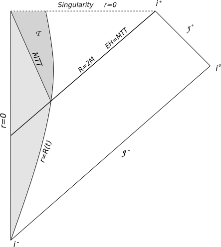
Figure 1: The Penrose diagram for $k=0$ dust collapse model of a black hole. The curve $r=R(t)$ shows the boundary of the dust cloud. The cloud reaches the singularity at $t=0$. All shells reach the singularity at the same time. The boundary of the cloud reaches the Schwarzschild radius at $t=-4M/3$. at exactly the same time, the null ray of event horizon also reaches that point. Once outside, the event horizon matches with the null marginally trapped tube (MTT). Furthermore, exactly at $t=-4M/3$, just as the cloud reaches its Schwarzschild radius, a timelike marginally trapped tube (MTT) forms and begins to shrink at the rate of $\dot{R}_{ah}=-3/2$ to reach the singularity at $t=0$. The region $\tau$ inside the cloud is the trapped region.

Let us now find the time development of the event horizon. Using the metric, we evaluate time evolution of radius along a radial null geodesic. The radial null geodesic of the outgoing photons give

$$\left(\frac{dr}{dt}\right)_{Null}=\frac{1}{R^{\prime}}.$$ (50)

Again, using $dR/dt=[R^{\prime}\left(dr/dt\right)_{Null}+\dot{R}]$, the time evolution of the event horizon reduces to:

$$\frac{dR}{dt} = 1-\sqrt{\frac{F}{R}}$$ (51)

Since $R(t)^{3/2}=(3/2)\sqrt{m}r^{3/2}(-t)$ and $F(r)=m\,r^{3}$, the previous equation gives:

$$\frac{dR}{dt} = 1+\frac{2}{3}\frac{\,R}{\,t}.$$ (52)

The solution of this equation gives the event horizon. The general solution of this equation is obtained by integrating with the integrating factor $t^{-2/3}$ and gives:

$$R_{eh}(t)=3t+C^{\prime}(-t)^{2/3}.$$ (53)

The constant $C^{\prime}$ is fixed as follows: From equation (47), the time taken by the shell to reach $R=2M$ is $t=-4M/3$. Since the event horizon is the last null ray reaching the null infinity, we use this condition in equation (53) to obtain $C^{\prime}=3(9M/2)^{1/3}$.

So, from equation (53), it follows that the event horizon begins to grow from the non- singular center just as the collapse process begins. The time of beginning of event horizon is obtained from equation (53) as follows: Let at $t=t_{eh}^{i}$, $R_{eh}=0$. This gives the time of formation of the event horizon $t_{eh}^{i}=-(9M/2)$. The rate of growth of the event horizon is also obtained from (53) and gives

$$\dot{R}_{eh}=3-2(9M/2)^{1/3}(-t)^{-1/3}.$$ (54)

This clearly shows that initially, at $t_{eh}^{i}$, $\dot{R}_{eh}=1$ whereas, at $t=-4M/3$, just as the shell reaches the Schwarzschild radius (or the null curve of the event horizon reaches $R=2M$), the event horizon stops growing, $\dot{R}_{eh}=0$ and remains at the Schwarzschild radius. To sum up, the event horizon begins to develop just as the matter shells begin to fall and then its rate of growth slows down as rate of fall of matter begins to slow down, ultimately stopping at time $t=-4M/3$ when matter flow stops and accordingly, it matches with the Schwarzschild null horizon (see fig. 1).

Example

In the following we shall consider the examples of a simple mass profile which shall collapse according to the formalism developed above. Let us consider the Misner- Sharp mass function to be $F(r)=mr^{3}$, with $m=(1/2)$. The $t-R(r,t)$ graph for the collapse is given below in figure 2. We have taken care to exclude shell- crossing singularities and have ensured that there are no trapped surfaces on the initial slice. Several points need to be noticed. First, all the shells collapse to the singularity at the same time at $t=0.94$. Second, the shell which begins at $R(r,t)=1$ reaches its Schwarzschild radius at time $t=0.61$, and exactly at that instant, the event horizon (or the last null- ray), beginning at the center of the cloud, also reaches that spacetime point. Thirdly, the MTT also forms at that point and eventually collapses to singularity, along with the matter cloud. Further, the graph of $C$ establishes that the MTT is timelike. Note that this graph is identical to figure 1, obtained for a generic mass profile.

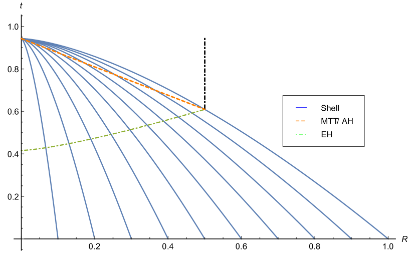
(a)

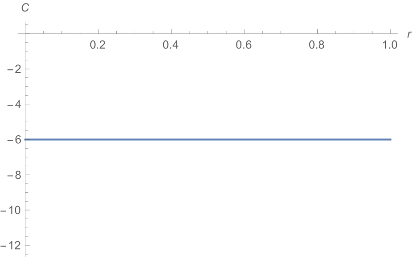
(b)

Figure 2: The figure (a) gives the plot of $R(r,t)$ vs $t$ for the mass profile discussed above. The MTT is timelike is also confirmed through the negative value of $C$ in the graph of $C-r$ in (b).

4.1.2 Bounded collapse

The line element of the interior metric (41) can be rewritten with the parameter $r=\sin{\chi}$ as

$$ds^{2}=-dt^{2}+a^{2}(t)\,d\chi^{2}+R(r,t)^{2}(d\theta^{2}+\sin^{2}{\theta}\,d\phi^{2}).$$ (55)

The parametric solution of the (40) for the $k>0$ is given by the following equations

$$R(r,t)=\frac{F(r)}{k(r)}\cos^{2}\left(\eta/2\right)=rm\cos^{2}\left(\eta/2\right),$$ (56)

$$t=\frac{F(r)}{2k(r)^{3/2}}\left(\eta+\sin\eta\right)=\frac{m}{2}\left(\eta+\sin\eta\right),$$ (57)

where $k(r)=r^{2}$ and $F(r)=mr^{3}$. The equation (56) shows that $a(t)=m\cos^{2}\left(\eta/2\right)$. Furthermore, the expressions for radius and time coordinates in (56) and (57) respectively show that collapse begins at $\eta=0$, where $t_{i}=0$ and it reaches the singularity, $R=0$ at $\eta=\pi$. Thus, the maximum value of the scale factor is $a(t=0)\equiv a_{0}=m$ at $\eta=0$ and the minimum value is $a=0$ at $\eta=\pi$, when the matter cloud reaches singularity. These relations are the same ones in [3] except that time has been shifted by ($\eta\rightarrow\pi-\eta$). A further interesting fact follows directly from equation (56), which may also be written as:

$$R(r,t)=(R_{0}/2)(1+\cos\eta).$$ (58)

Consequently, the time taken by the shell initially at $R_{0}=(rm)$ to reach it’s Schwarzschild radius at $R=2M$ is given by:

$$\eta_{2M}=\cos^{-1}\left(4M/R_{0}-1\right).$$ (59)

This is exactly the same moment where the apparent horizon starts forming.

Now, recall that to an outside observer, the collapse process only leads to a Schwarzschild spacetime. Hence, the metric of the cloud interior (FRW) must be matched with the Schwarzschild spacetime in the exterior. This matching at the junction, of the metric function and the extrinsic curvatures (in particular, $K_{\theta\theta}$) give us the following conditions respectively:

$$R(t)=a(t)\sin\chi$$ (60)

$$2M=F(r),$$ (61)

where $M$ is the total mass enclosed by the shell. At the beginning of the shell collapse (at $\eta=0$), these conditions imply that

$$R(t=0)\equiv R_{0}=m\sin\chi_{0},~{}~{}~{}~{}~{}~{}~{}~{}~{}~{}~{}2M=F(r_{0}),$$ (62)

where $r_{0}=\sin\chi_{0}$ is the radial coordinate of the shell boundary at the beginning of the collapse. From the above two equations, it follows simply that

$$\chi_{0}=\sin^{-1}\left(2M/R_{0}\right)^{1/2},~{}~{}~{}~{}~{}~{}~{}~{}~{}~{}~{}~{}a_{0}=m=\left[R_{0}^{3}/(2M)\right]^{1/2}.$$ (63)

We shall label the shell by the radial coordinate it has at $\eta=0$. The time for the collapsing shells labeled by ’$r$’ to reach the central singularity $R=0$ is given by

$$t_{s}=\frac{\pi F(r)}{2k(r)^{\frac{3}{2}}}=\frac{\pi}{2}m.$$ (64)

From equation (64), $t_{s}=(\pi m/2)$ is constant and hence, all collapsing shells with different initial radius will reach the central singularity at the same time.

Let us have a look at the trapped surfaces and identify the trapped region. For spherical symmetry, the outermost trapped surface is identified through the equation $R(t,r)=F(r)$. From equation (56), we get $\eta=2\cos^{-1}[R(r,t)k/F(r)]^{1/2}$ and hence, the AH/MTT is described by

$$\eta_{AH}=2\cos^{-1}r=2\cos^{-1}\,(\,\sin\chi\,)=\pi-2\,\chi.$$ (65)

Thus, for a shell labeled by $r_{0}$ or $\chi_{0}$, the AH/MTT forms at the time given by the coordinates:

$$\eta_{AH}=\pi-2\chi_{0}=2\cos^{-1}\left(2M/R_{0}\right)^{1/2}=\cos^{-1}\left(4M/R_{0}-1\right),$$ (66)

where we have used the trigonometric identity $\cos^{-1}x=(1/2)\cos^{-1}(2x^{2}-1)$. This equation clearly shows as clouds of larger and larger initial radius $R_{0}$ are considered, their AH form at later times. Furthermore the time of formation of the horizon is exactly same as the time when the cloud reaches it’s Schwarzschild radius, given in equation (59). These equations also imply that inside the matter cloud, radius of the AH decreases at a constant rate. This follows simply because, for a shell of fixed $r$, the rate of decrease of radius of AH is equivalent to finding $da/d\eta$. It is easy to see from $a(\eta)=m\cos^{2}\left(\eta/2\right)$ and the equation (65) that it is indeed a negative constant inside the matter. Using the previous equation in (57), we may also find the time curve of the apparent horizon:

$$t_{ah}=(m/2)\left(\pi-2\chi+\sin\,2\chi\right).$$ (67)

Another way to determine the trapped region is to use it’s definition, that light rays remain confined in this strong gravitational field and the proper area of this bundle of light rays do not grow with time. To use this formulation, let us go to the the proper time coordinates $\eta$ given through equation $\eqref{tk=1}$. In the $(\eta-\chi)$ coordinates, the light rays are given by the equation $(d\chi/d\eta)=1$. Now, for the metric (55), apart from a constant $4\pi$, the total area is $A=a^{2}\sin^{2}\chi$ and also, from equation (56), it follows that $da=-(m/2)\sin\eta\,d\eta$. Thus, we get that the variation of the area along vector field $(\partial/\partial\eta)$ of proper time coordinate $\eta$ is:

$$\pounds_{\eta}\,A = \frac{da}{d\eta}\sin\chi+a\cos\chi\frac{d\chi}{d\eta}$$ (68)

$$= -m\sin\chi\sin[\eta/2]+m\cos[\eta/2]\cos\chi=m\cos\left[\frac{\eta}{2}+\chi\right].$$

Using $\cos(\pi/2)=0$, the expression for non- increase of area, given by $(dA/d\eta)\leq 0$ translates to [49]:

$$\eta\geq\pi-2\chi,$$ (69)

where the inequality signifies trapped region and the equality gives boundary of the trapped region, also called marginally trapped tube or apparent horizon. Note that this equation (69) is exactly same as the one derived in eqn. (65) using different methods.

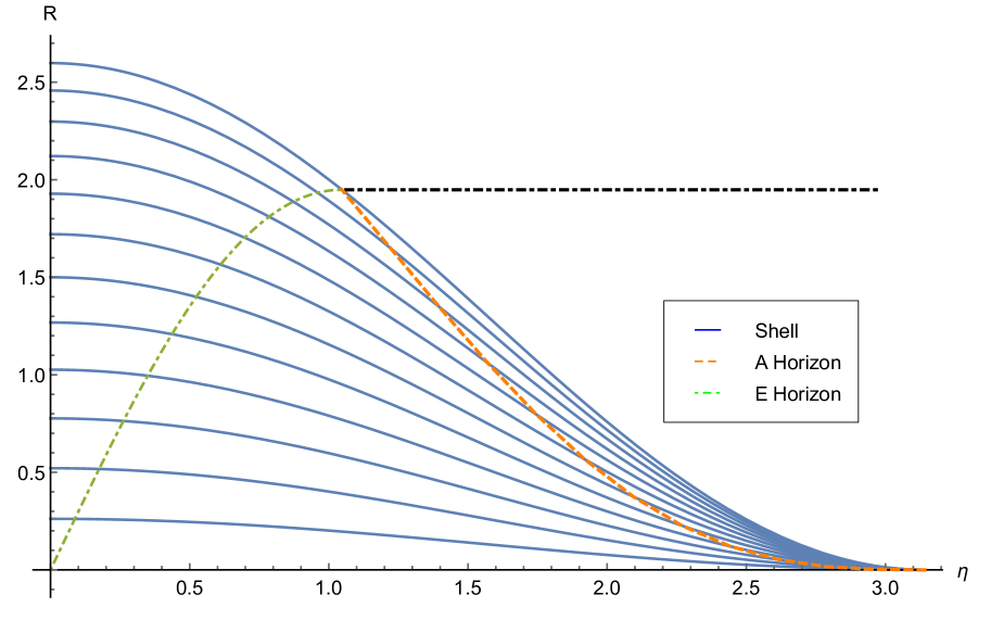
(a)

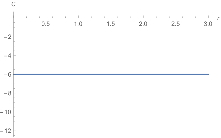
(b)

Figure 3: Plot of collapsing shell (solid line), MTT (or apparent horizon) (dashed line) and event horizon (dot- dashed) with respect to $\eta$. For OSD model, the equations are given for collapsing shells in (56), for apparent horizon in (65) and for event horizon (72). We consider the matching of interior to the exterior at the hypersurface $\chi_{0}=\pi/3$ where $r_{0}=0.866$. For simplicity, each collapsing shell has the constant mass $m=3$ for which the Schwarzschild radius is formed at $\left(\eta_{2M},R_{2M}\right)=\left(1.0472,2\right)$. All three curves collapsing shell, apparent horizon and event horizon meet at $R=2$ when $\eta_{{}_{2M}}=1.0472$. Here too, the MTT is timelike as may be observed from the graph of $C$ given above in (b) and hence, it is unstable.

Now we also want to study the formation and evolution of the event horizon, more precisely identify when and where it first starts forming and how it grows with time. Again, we shall need the null geodesics since event horizon is also the last ray that reaches the asymptotic null infinity $\mathcal{I}^{+}$. The outgoing radial null geodesics in the $(r,t)$ coordinates are given by

$$\frac{dr}{dt}=\frac{\sqrt{1-k(r)}}{R^{\prime}}=\frac{\sqrt{1-r^{2}}}{m\cos^{2}\left(\eta/2\right)}.$$ (70)

We shall however use the $(\chi-\eta)$ coordinates in which this equation becomes $(d\chi/d\eta)=1$. Now, we use the boundary condition that at the instant the the cloud reaches the Schwarzschild radius, the last outgoing null geodesic also reaches that point at that same instant. For example, just as the shell with initial radius $R_{0}=m\sin\chi_{0}$ (labelled by $R_{0}$ or $r_{0}$ or $\chi_{0}$) reaches the Schwarzschild radius ($R=2M$), the event horizon also reaches there at that instant. So, for this shell, the boundary condition is $\chi=\chi_{0}$ at $\eta=\eta_{AH}=\eta_{2M}$. In other words, the coordinates of the event horizon is given by:

$$\chi_{EH}=\chi_{0}+(\eta-\eta_{2M}).$$ (71)

Using equation (56), the equation of the last outgoing null ray inside the cloud with initial radius $R_{0}$ is given by

$$R_{EH} = mr_{EH}\cos^{2}\left(\eta/2\right)=m\sin\left(\chi_{0}+\eta-\eta_{2M}\right)\,\cos^{2}\left(\eta/2\right).$$ (72)

Note that just as the shell (of radius $R_{0}$) begins to collapse, the event horizon also begins to form at $\eta=(\eta_{2M}-\chi_{0})$ and grows in such a way that at $\eta=\eta_{2M}=(\pi-2\chi_{0})$, it’s value reaches $R_{EH}=m\sin\chi_{0}\cos^{2}\left(\pi/2-\chi_{H}\right)=m\sin^{3}\chi_{0}=2M$. Also, we can find the rate of growth of the event horizon from equation (72) by taking the derivative with the proper time $\eta$,

$$\frac{dR_{eh}}{d\eta}=m\cos\left[3\left(\chi_{0}+\eta/2\right)-\pi\right]\cos\left(\eta/2\right)$$ (73)

where we have used $\eta_{2M}=\pi-2\chi_{0}$. So, the event horizon grows at a positive rate and at $\eta=\eta_{2M}$, it becomes $dR_{EH}/d\eta=0$ and hence, it stops growing and matches with the outermost trapped surface of the Schwarzschild spacetime. These results are summarised in the figure 3.

Example

In this example, we consider the density of the cloud to be of the following form [44]:

$$\rho(r)=\frac{m_{0}\,\mathcal{E}(\varsigma)}{r_{0}^{3}}\left[1-\operatorname{Erf}\left\{\varsigma\left(\frac{r}{r_{0}}-1\right)\right\}\right],$$ (74)

where $m_{0}=m(r\rightarrow\infty)$ is the total mass of the cloud, $r_{0}$ is the location on the cloud where it matches the Schwarzschild radius ($r_{0}=2m_{0})$, and the quantity $\varsigma$ controls the approach to the OSD model- larger the value of $\varsigma$, closer is the density to uniformity. The function $\mathcal{E}(\varsigma)$ has the following form:

$$\mathcal{E}(\varsigma)=3\varsigma^{3}\,\left[2\pi\varsigma(2\varsigma^{2}+3)(1+\operatorname{Erf}\varsigma)+4\sqrt{\pi}\exp(-\varsigma^{2})(1+\varsigma^{2})\right]^{-1},$$ (75)

and $\operatorname{Erf}$ is the usual error function. We consider the cases where $\varsigma=1,5$ and $15$. The graphs are given in figure 4.

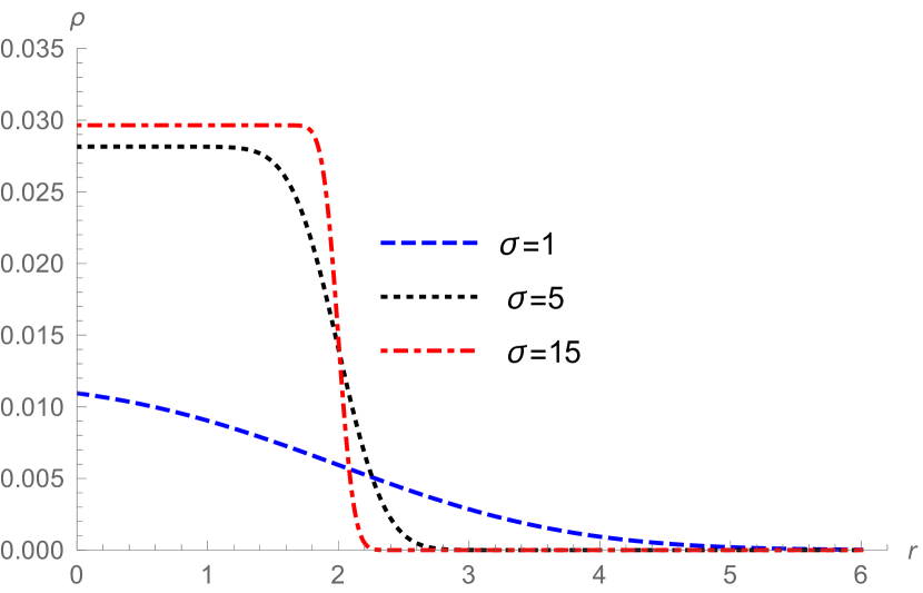
(a)

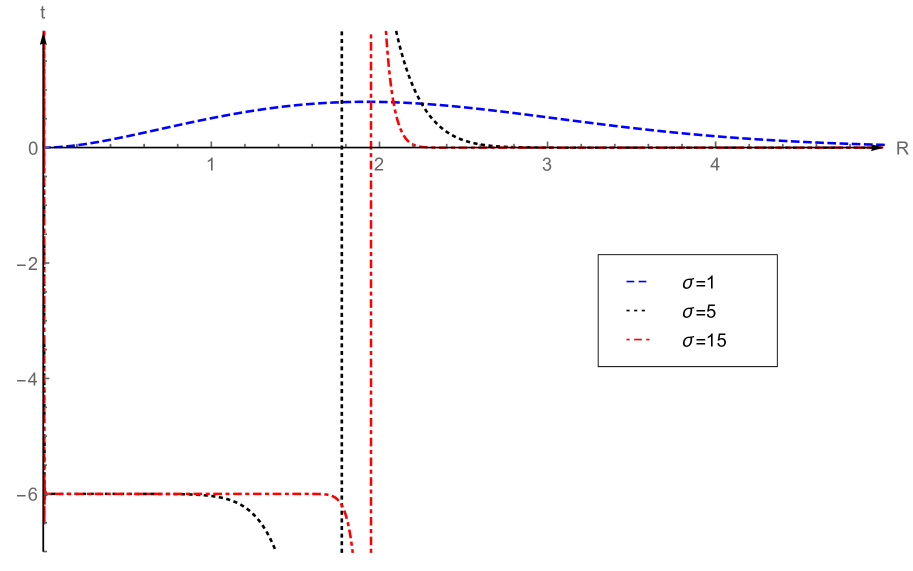
(b)

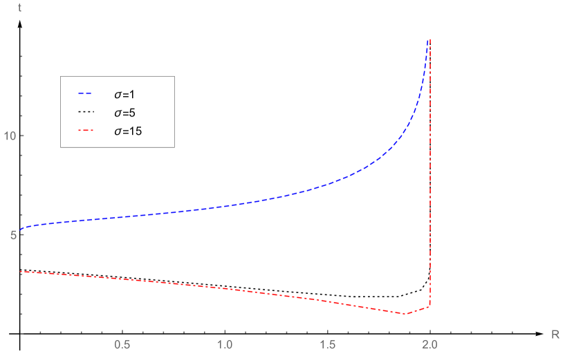
(c)

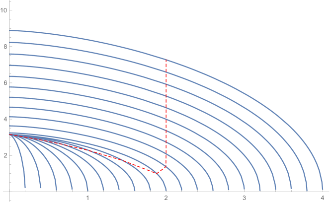
(d)

Figure 4: This gives the gravitational collapse for the OSD profile discussed above where (a) gives the density fall-off, (b) gives the values for $C$, (c) gives the formation of MTT for $\varsigma=1,5,15$. The graph (d) shows the MTT for $\varsigma=15$ along with the shell coordinates. The straight lines in (c) and (d) represents the isolated horizon phase.

As seen from the graph of the density profile, the density approaches the step function as $\varsigma$ varies from $1$ to $15$. For larger values of $\varsigma$, the density is a step function. The $R(r,t)$ vs $t$ graphs for these various choices of $\varsigma$ are also plotted. We have ensured that the parameter space does not have shell- crossing singularities and that the initial time slice does not admit any trapped region. From the $R(r,t)-t$ graph for $\varsigma=15$ (which is closest among these to the OSD model), we note that the MTT forms at approximately $t=0.99$ and $R=1.88$. Wherefrom, the MTT bifurcates into two parts: the timelike membrane collapses to the center of the cloud, while the dynamical horizon asymptotes to the isolated horizon at $R=2$. The timelike nature of the MTT, and it’s approach to null through the spacelike phase may also be confirmed through the $C-r$ graph. This graph shows that for smaller $r$ the signature of MTT is negative, which jumps to $+$ve at $r=1.99$ and eventually becoming null at approximately $r=2.3$. Note that these changes are also corroborated through the graphs of density $\rho(r)-r$ as well as that of $R(r,t)$ vs $t$. For lower values of $\varsigma$, the MTT forms at lower values of $R(r,t)$. For example, for $\varsigma=5$, the MTT forms at $t=1.88$ and $R=1.62$. The $C$ value also remains $-$ve initally but asymptotes to $0$ as it becomes isolated. For $\varsigma=1$, the situation is drastically different since, it cannot be called to represent the OSD model. Here, the MTT is spacelike, which may also be confirmed from the values of $C$ in the figure below.

4.1.3 Unbounded collapse

The forms of the Einstein equations takes simplified form for dust collapse with $k<0$ when we use the parametric form of $R$ or $a(t)$. The line element of the interior metric (41) can be written with $r=\sinh{\chi}$ as

$$ds^{2} = -dt^{2}+\frac{R^{\prime 2}}{1+k(r)}{dr^{2}}+R^{2}\left(d\theta^{2}+\sin^{2}{\theta}d\phi^{2}\right)$$ (76)

The parametric solution of the (40) for the $k<0$ is

$$R(r,t) = \frac{F(r)}{2|k(r)|}\left(\cosh\eta-1\right),$$ (77)

$$t(\eta) = \frac{F(r)}{2|k(r)|^{3/2}}\left(\sinh\eta-\eta\right)$$ (78)

where $k(r)=-r^{2}$ and $F=mr^{3}$. This is the case for unbounded collapse and hence, the shells begin at some fixed time and follows the collapse process. The collapse starts at $\eta=\eta_{0}$, where $t=t_{0}=(m/2)(\sinh\eta_{0}-\eta_{0})$ and $R_{0}\equiv R(r,t=t_{0})=(rm/2)(\cosh\eta_{0}-1)\equiv rm\alpha$, and it reaches the singularity at $\eta=0$ at $t=0$ where $R=0$. Again, these are the same equations as in [3] with the time coordinate shifted.

We may rewrite the equation (77) to obtain the equation of motion of the shell:

$$R(t,r)=(R_{0}/2\alpha)(\cosh\eta-1),$$ (79)

and hence, the shell of initial radius $R_{0}$ reaches its Schwarzschild radius $R=2M$ at the proper time

$$\eta_{2M}=-\cosh^{-1}(4M\alpha/R_{0}+1).$$ (80)

The sign has been kept $-$ve since the $\eta=0$ is the singularity time and the shell must reach it’s Schwarzschild radius before that time. Also note that at $t_{s}=0$, the collapsing shells reach the central singularity $R=0$. Thus, all shells with different initial radius will reach the central singularity at the same time.

Similar to the junction conditions for the previous two cases, here too the matching of the metric and the extrinsic curvatures for FRW spacetime inside the cloud with the Schwarzschild spacetime outside the cloud leads respectively to these equations:

$$R(t,r)=a(t)\sinh\chi,~{}~{}~{}2M=F(r).$$ (81)

So, at the beginning of the collapse of the shell with initial radius $R_{0}$, these conditions imply that the following two relations hold:

$$R_{0}=m\alpha\sinh\chi_{0},~{}~{}~{}~{}~{}~{}2M=F(r_{0})=m\sinh^{3}\chi_{0},$$ (82)

where $r_{0}=\sinh\chi_{0}$ is the radial coordinate of boundary of the cloud at the beginning of the collapse. Thus, we rewrite these two equations as:

$$\chi_{0}=\sinh^{-1}(2M\alpha/R_{0})^{1/2},~{}~{}~{}~{}~{}~{}m=[R_{0}^{3}/2M\alpha^{3}]^{1/2}.$$ (83)

Let us now look at the formation of the trapped surfaces and in particular for MTT/AH. From equation (77), we have $\eta=\cosh^{-1}[(2R(r,t)k/F)+1]$ and hence, the time of formation of AH is obtained by using the condition $R(r,t)=F(r)$ correspondingly, the time is: $\eta=\eta_{AH}=\cosh^{-1}(2r^{2}+1)=\cosh^{-1}(2\sinh^{2}\chi+1)=-2\chi$. This just shows that the AH forms much before the shells reach the singularity. For a shell labeled by $r_{0}$, $\chi_{0}$ or the starting radius $R_{0}$, the apparent horizon forms at the time ($-2\chi_{0}$):

$$\eta_{AH}=-2\sinh^{-1}(2M\alpha/R_{0})^{1/2}=-\cosh^{-1}(4M\alpha/R_{0}+1),$$ (84)

where we have used equation (83) and the inverse hyperbolic identity $2\sinh^{-1}x=\cosh^{-1}(2x^{2}+1)$, for $x>0$. This shows that the apparent horizon forms at exactly the same time when the matter cloud reaches it’s Schwarzschild radius, given by equation (80).

Similar to the calculations in the previous subsection, we also may formulate the problem of trapped surface by looking at the change of the $2$- sphere areas with proper time. The outgoing null geodesics will be trapped if their proper area do not grow with time. For the metric (76), the area is also written (apart from some factors of $4\pi$) as $A=a^{2}(\eta)\sinh^{2}\chi$.

From equation (77), $a(\eta)=m\sinh^{2}(\eta/2)$ and hence $da=(m/2)\sinh\eta\,d\eta$ and also $(d\chi/d\eta)=1$ thus,

$$\frac{dA}{d\eta} = \frac{da}{d\eta}\sinh\chi+a\cosh\chi\frac{d\chi}{d\eta}=\sinh\left(\eta/2+\chi\right)\leq 0$$ (85)

This implies that the time of formation of the AH/MTT is obtained from the equality $\eta_{AH}=-2\chi$ whereas, the points for which the inequality is satisfied forms the trapped region. This exactly matches with the expression of time of formation of apparent horizon derived before.

Let us now check the time of formation of the event horizon. Just as the matter shell starts to fall, outward directed null rays also begin to proceed towards the asymptotic null infinity. The event horizon is the last outward directed null ray that reaches the infinity. The outward directed null rays, in the $(\eta-\chi)$ coordinates, are given by the equation $(d\chi/d\eta)=1$. Let us use the boundary conditions that just as the shell with labeled by $R_{0}$ reaches its Schwazschild radius ($R=2M$), the null ray of the event horizon also reaches there. This is given in the form $(\chi=\chi_{0})$ at $\eta=\eta_{2M}$. This gives the equation

$$\chi_{EH}=\chi_{0}+(\eta-\eta_{2M}).$$ (86)

Just as the cloud of initial radius begins to fall, the event horizon also starts to grow inside the cloud. The equation for the radius of the event horizon is given by:

$$R_{EH} = mr_{EH}\sinh^{2}(\eta/2)=m\sinh(\chi_{EH})\sinh^{2}(\eta/2)$$ (87)

$$= m\sinh(\chi_{0}+\eta-\eta_{2M})\sinh^{2}(\eta/2).$$

Notice that at $\eta=\eta_{2M}=-2\chi_{0}$, $R_{EH}=m\sinh^{3}\chi_{0}=2M$, which implies that at $\eta=-2\chi_{0}$, the event horizon matches with the Schwarzschild radius of the shell. Next, we also show that the matching is smooth and the rate of growth of the event horizon becomes zero at that $\eta=\eta_{2M}=-2\chi_{0}$. This is obtained as follows:

$$\frac{dR_{eh}}{d\eta}=m\sinh(\eta/2)\,\sinh[(3\eta/2)+\chi_{H}-\eta_{2M}].$$ (88)

So, it follows that at $\eta=\eta_{2M}=-2\chi_{0}$, $(dR_{EH}/d\eta)=0$. The behaviour of the graphs of the EH, MTT and the shells may also be studied here. The nature is similar to the previous two cases, we skip them.

4.2 Inhomogeneous collapse

For the inhomogeneous collapse, the $\alpha=\alpha(t)$ in the metric and may again be absorbed through the redefinition of the time coordinates, see equation (38). The mass function still remains a function of $r$ only and is taken to be of the form $F(r,t)=r^{3}m(r)$ and the metric function is given by $k(r)=K(r)\,r^{2}$.

4.2.1 Marginally bound collapse

The marginally bounded collapse corresponds to $K=0$. The metric is given by

$$ds^{2}=-dt^{2}+R^{\prime\,2}(r,t)\,dr^{2}+R^{2}(r,t)(d\theta^{2}+\sin^{2}\theta\,d\phi^{2}),$$ (89)

where $R(r,t)$ is the radius of the shell. The equation of motion of the shell is given by

$$\dot{R}^{2}=F(r)/R.$$ (90)

The solution of the equation of motion is given by the following form:

$$t=(2/3)\left[\sqrt{r^{3}/F}-\sqrt{R(r,t)^{3}/F}\right],$$ (91)

where the radius of the shell at the beginning of the collapse at $t_{i}=0$ is $R(r,t_{i})=r$. The shells will be labeled by the value of the radius it assumes at the initial time $t=0$. For example for the shell being studied above, it shall be labeled by the coordinate $r$. For this shell, labeled by the coordinate $r$, the time taken for it to reach the singularity is

$$t_{s}=(2/3)r^{3/2}/\sqrt{F}.$$ (92)

Note that since $F(r)$ is inhomogeneous, all shells do not reach the singularity at the same time. The equation of motion given above for the shell may naturally be rewritten as:

$$t=t_{s}-(2/3)\sqrt{R(r,t)^{3}/F}.$$ (93)

Let us, for simplification, shift the time coordinate and use the choice $t_{s}=0$. With this simplification, the time for the shell to reach $R=2M$ is given by $t_{2M}=(-4M/3)$. The equation of the trapped surface is obtained by using the condition $R(r,t)=F(r)$ giving the equation for MTT/AH as:

$$R_{AH}(r,t)=-(3/2)\,t.$$ (94)

This equation clearly implies that the AH/MTT begins at $R=2M$, shrinks at a constant rate of $\dot{R}_{AH}=-(3/2)$, and goes to zero at the same time when the singularity forms. The apparent horizon which is outside the shell, matches with the Schwarzschild null event horizon. Note that the slope of the $R_{AH}(r,t)-t$ graph is negative. However, this does not mean that the AH/MTT is timelike. In the examples that follow, we shall show that even if the MTT behaves as a timelike curve in the $R(r,t)-t$ graph, it is the constant $C$ which fixes the signature of MTT [44, 70].

Let us now look at the formation of the event horizon, for which we need to look at the radial null geodesic, given by the curve $R[r,t_{n}(r)]$. The event horizon shall be obtained by tracing the last radial null geodesic reaching the null infinity. The tangent vector field to this curve is given by:

$$\frac{dR}{dt}=\dot{R}+R^{\prime}\,\left(\frac{dr}{dt}\right)_{null},$$ (95)

where the radial null geodesic, as given in the second term on the right side of the above equation, for $k=0$, is given by $(dr/dt)_{null}=(1/R^{\prime})$. This gives us $(dR/dt)=(1+\dot{R})$. From the equation (90), this gives us:

$$\frac{dR}{dt}=1-\sqrt{\frac{F}{R}},$$ (96)

Using, form equation (93), the fact that $F(r)=(2/3)R^{3}(-t)^{-2}$, the above equation is reduced to the form:

$$\frac{dR}{dt}=1+\frac{2R}{3t}.$$ (97)

with the solution $R(r,t)=3t+C^{\prime}\,t^{2/3}$, where $C^{\prime}$ is a constant of integration. The constant $C^{\prime}$ may be set by the condition that, at the time when the shell reaches its Schwarzschild radius ($R=2M$), the null geodesic also reaches that point at exactly the same time. This gives the equation of curve of the event horizon:

$$R_{EH}=3t+3(9M/2)^{1/3}\,(-t)^{2/3}.$$ (98)

Note that just as in the case for homogeneous collapse, the event horizon begins just as the matter shells begin to fall, growing slowly to smoothly match with the Schwarzschild horizon at $R=2M$ at $t=-4M/3$. At that time, the rate of growth of $R_{EH}$ vanishes and for $t\geq-4M/3$, the event horizon is the null Schwarzschild horizon of radius $2M$.

Examples:

Here, we shall consider two examples, with the densities having the following forms:

$$\rho_{1}(r)=(3M/2500)(10-r)\,\Theta(10-r),$$

$$\rho_{2}(r)=(3M/40\sqrt{10})(10-r^{2})\,\Theta(10-r^{2}),$$ (99)

where $\Theta(x)$ denotes the Heaviside theta function. The factors have been chosen to get the isolated horizon at $R(r,t)=2$ and the corresponding masses have been normalised with the choice $M=1$. In each of these cases the MTT are spacelike, as indicated by the values of $C$. Again, there are no shell- crossing singularities and no trapped surfaces on the initial slice. The $R-t$ plots however are intricate in these two cases and are markedly different (see figures 5 and 6). We give each of these two cases since they show the non- trivial ways in which the MTTs cross the foliation. For the density profile corresponding to $\rho_{1}$, the MTTs are spacelike.

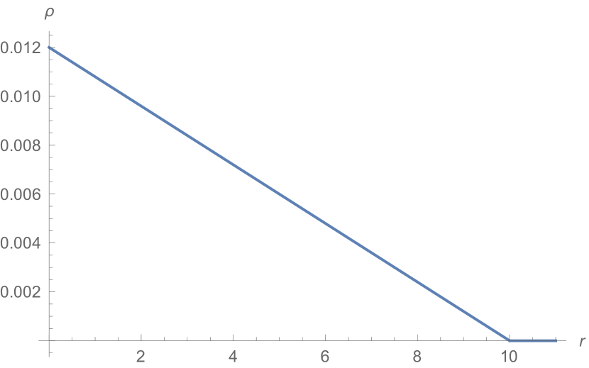
(a)

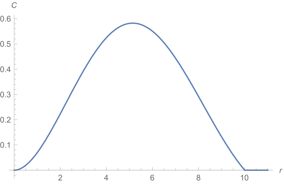
(b)

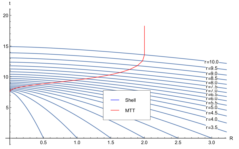
(c)

Figure 5: The graphs show the (a) density distribution $\rho_{1}$, (b) values of $C$, and (c) formation of MTT along with the shells. The MTT begins from the center of the cloud. The straight lines of MTT in (c) after the shell $r=10$ has fallen, represents the isolated horizon phase.

As seen from the $R(r,t)-t$ graph, the MTT forms out of the central singularity, evolves in a spacelike manner and approaches the isolated horizon phase at $R=2$. Although it may seem from these graphs that timelike membranes arise here, that it is not so may be verified from the graphs of $C$. This bending of graphs only indicates that the MTTs cross the foliation is intricate ways [44, 70].

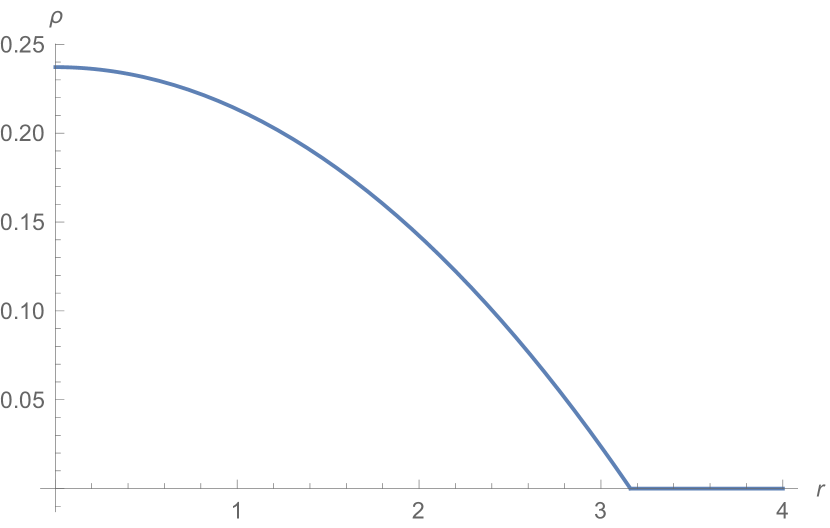
(a)

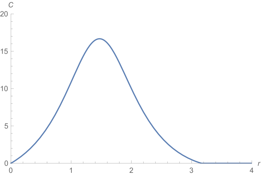
(b)

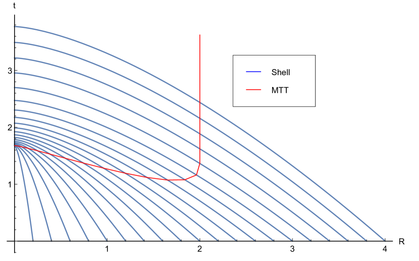
(c)

Figure 6: The graphs show the (a) density distribution $\rho_{2}$, (b) values of $C$, and (c) formation of MTT along with the shells. Note that the MTT seems to begin at $r=2.6$ and then bifurcates in a timelike manner to the singularity while another part proceeds towards the isolated horizon. However, since the signature of $C$ is always positive, the behavior of the MTT must be like that in figure 5. The timelike nature arises due to non-trivial intersection with the foliation [44, 70].

4.2.2 Bounded collapse

For the case of bounded collapse, $k(r)>0$, the parametric solutions are given by:

$$R(r,t) = \frac{F(r)}{k(r)}\cos^{2}\left(\eta/2\right)=r\cos^{2}\left(\eta/2\right)$$ (100)

$$t = \frac{F(r)}{2k(r)^{3/2}}\left(\eta+\sin\eta\right)=\frac{r^{3/2}}{\sqrt{F}}\left(\eta+\sin\eta\right),$$ (101)

where we assume the function $k(r)$ to be of the form $k(r)=F(r,t)/r$, with $F(r,t)=m(r)r^{3}$.

The collapse of the cloud begins at $\eta=0$, where $t=t_{i}=0$ and $R(r,t_{i})=r$ and reaches the singularity at $\eta=\pi$ where $R=0$. Note that the time for collapsing shells labeled by r to reach the central singularity $R=0$ is

$$t_{s}=\frac{\pi F(r)}{2\,k(r)^{3/2}}=\frac{\pi}{2m(r)^{1/2}}$$ (102)

It follows clearly from this equation (102), $t_{s}$ is not a constant (unlike the OSD collapse). So, shells with different initial radius will reach the central singularity at different times. From equation (100), we have $\eta=2\cos^{-1}(Rk/F)^{1/2}$ and hence, the proper time for the shell to reach the Schwarzschild radius $R=2M$ is correspondingly given by $\eta_{2M}=2\cos^{-1}(2M/r)^{1/2}$.

Let us now locate the AH/MTT, which for spherical symmetry, is denoted by the condition $R(t,r)=F(r,t)$. From equations (100) and (101), the equations for formation of trapped surfaces are given by:

$$R_{ah} = r_{ah}\cos^{2}\left(\eta_{ah}/2\right)$$ (103)

$$t_{ah} = \frac{1}{2[m(r_{ah})]^{1/2}}\left(\eta_{ah}+\sin{\eta_{ah}}\right).$$ (104)

In order to find $r_{ah}$, we use the trapping equation $R=F$. Taking derivative on both sides we have

$$\frac{dr_{ah}}{dt} = \frac{\dot{R}}{F^{\prime}-R^{\prime}}.$$ (105)

To obtain the derivatives appearing in the above equation, we use the equations (100) and (101) and get, after some straightforward simplifications, a complicated looking expression, relating the change of the shell radius of the AH with respect to proper time $\eta$:

$$\frac{dr_{ah}}{d\eta} = -\frac{(\sin\eta)/2+(1-k/k)^{1/2}\cos^{2}(\eta/2)}{D},$$ (106)

where the denominator $D$ is given by the following form:

$$D = (kF^{\prime}/F)-\left[(F^{\prime}/F)-(k^{\prime}/k)\right]\cos^{2}\eta/2$$ (107)

$$~{}~{}~{}~{}~{}~{}~{}~{}~{}~{}~{}~{}~{}~{}~{}~{}~{}~{}~{}~{}+[(1-k)/4k]^{1/2}\left(F^{\prime}/F-3k^{\prime}/2k\right)\left[\eta+\sin(\eta)\right].$$

Using the solutions of (106) into (103),(104) gives the equation of the trapped surfaces/apparent horizon. Also from equation (104), at this same time, the apparent horizon should be at $R=2M=F$.

These equations also give the evolution of event horizon. Just as in the previous sections, we determine the outgoing radial null geodesics which are given by

$$\frac{dr_{eh}}{dt} = \frac{[1-k(r)]^{1/2}}{R^{\prime}}$$ (108)

Now using the equations (100) into the above equation (108) we have

$$\frac{dr_{eh}}{d\eta} = -\frac{(\sin\eta/2)+(1-k/k)^{1/2}\cos^{2}(\eta/2)}{\bar{D}}$$ (109)

where the denominator $\bar{D}$ is given by the following form:

$$\bar{D} = \left[(F^{\prime}/F)-(k^{\prime}/k)\right]\cos^{2}\eta/2$$ (110)

$$~{}~{}~{}~{}~{}~{}~{}~{}~{}~{}~{}~{}~{}~{}~{}~{}~{}~{}~{}~{}-[(1-k)/4k]^{1/2}\left(F^{\prime}/F-3k^{\prime}/2k\right)\left[\eta+\sin(\eta)\right].$$

We have considered $(r_{H},\eta_{2M})$ to be the point where outer event horizon forms. Thus the equation of the interior event horizon is given by

$$R_{eh} = r_{eh}\cos\left[\frac{\eta}{2}\right]^{2}$$ (111)

We have used numerical integration to solve the above equations (106) and (109). We have all the required equations to study the LTB collapsing shells (100), apparent horizon (103) and event horizon (111). Where we have consider that the matching of interior to the exterior is done at the hypersurface when $\chi_{{}_{H}}=\pi/3$, $r_{H}=0.866$ and $m(r)=(n_{0}+rn_{1})$, such that the point where exterior even horizon formed is $\left(\eta_{2M},R_{2M}\right)=\left(2.1399,2.0\right)$. Thus all three curves collapsing shell, apparent horizon and event horizon should meet at $R=2.0$ when $\eta_{{}_{2M}}=2.1399$ for $n_{0}=1/11$ and $n_{1}=1/4$.

Examples:

(i)Let us consider the case where the density is given by

$$\rho(r)=(3M/5000)(100-r^{3})\,\Theta(100-r^{3}).$$ (112)

For this density profile too, the MTT is spacelike.

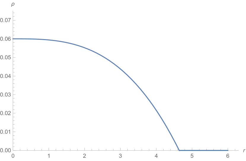
(a)

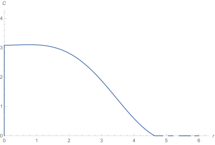
(b)

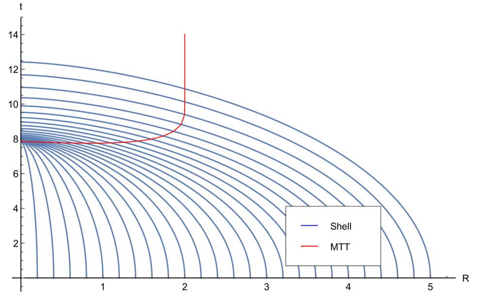
(c)

Figure 7: The graphs show the (a) density distribution, (b) values of $C$, and (c) formation of MTT along with the shells. The MTT begins from the center of the cloud. The straight lines of MTT in (c), after approximately $r=4.6$, represents the isolated horizon phase.

This may be confirmed though the $C-r$ graph (see the figures in 7). The $R-t$ graph shows that it develops from the center of the cloud and evolves in a spacelike manner to reach the isolated horizon at $R=2$. Although the graph may look to have a timelike evolution in the $R-t$ graph, it is due to the choice of foliation as explained above.

(ii)Let us consider a Gaussian profile with the density given by the following form [44]:

$$\rho(r)=\frac{m_{0}}{\pi^{3/2}r_{0}^{3}}\exp(-r^{2}/r_{0}^{2}),$$ (113)

where $m_{0}$ is the total mass of the matter cloud, $r_{0}$ is a parameter which indicates the distance where the density of the cloud decreases to $[\rho\,(0)/e]$.

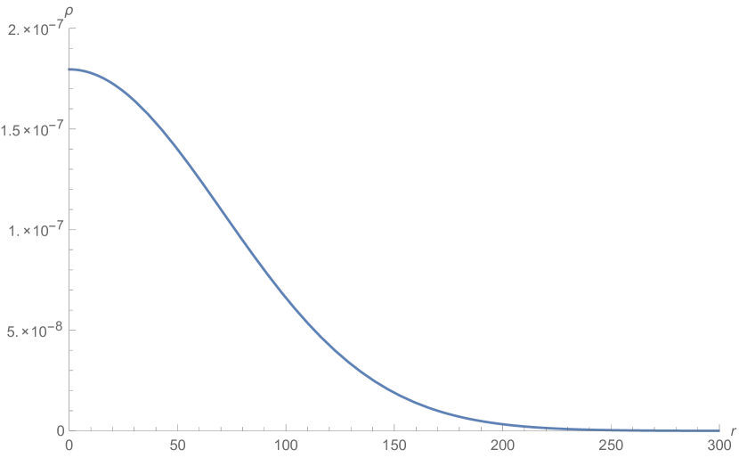
(a)

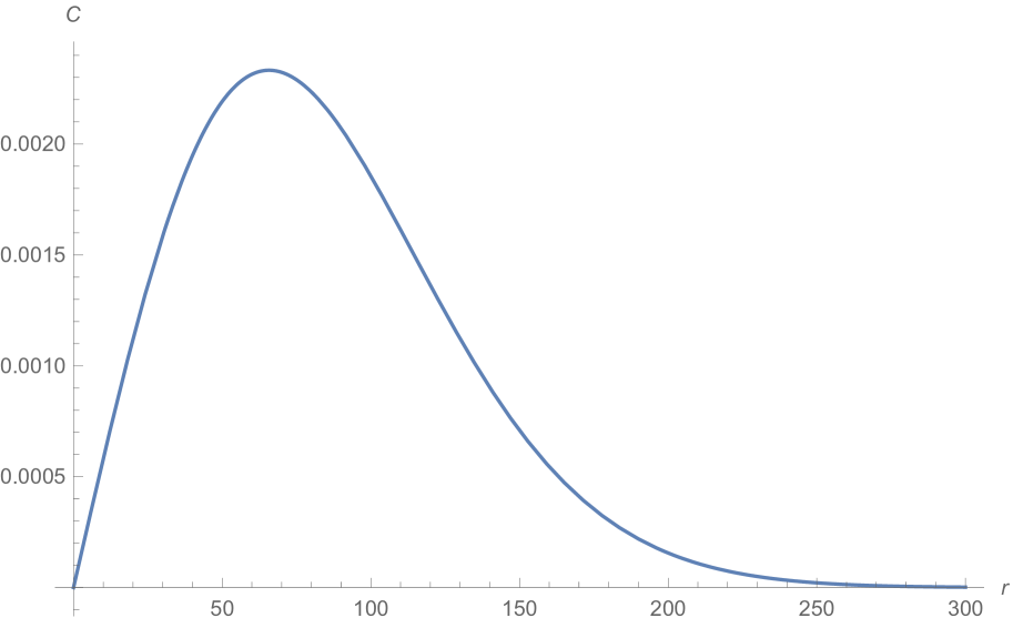
(b)

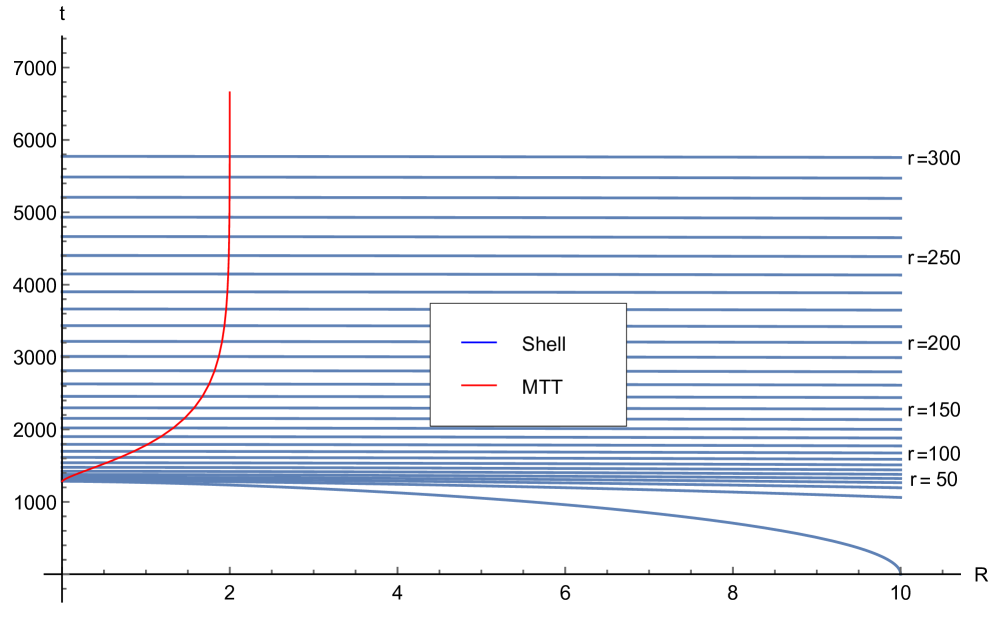
(c)

Figure 8: The graphs show the (a) density distribution, (b) values of $C$, and (c) formation of MTT along with the shells. The MTT begins from the center of the cloud. The straight lines of MTT in (c), after the shell $r=250$, represents the isolated horizon phase.

In our example, we have chosen $r_{0}=100\,m_{0}$. As usual, the MTT begins from the central singularity, and develops as a dynamical horizon until at approximately $r=200$, is begins to resemble an isolated horizon (see figure 8). This may also be confirmed from the fact that the density at $r=200$ is almost negligible. However, since the Gaussian profile almost disappears at $r=380$, the $R=2$ is also reached at that value of the shell coordinates.

(iii) Let us consider another density profile with the following form:

$$\rho(r)=\frac{m_{0}}{8\pi r_{0}^{3}}\exp(-r/r_{0}),$$ (114)

where $m_{0}$ is the total mass of the matter cloud, $r_{0}$ is a parameter which indicates the distance where the density of the cloud decreases to $[\rho\,(0)/e]$.

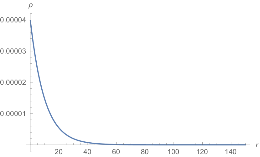
(a)

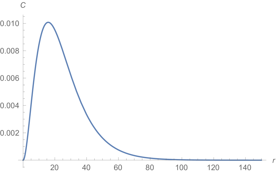
(b)

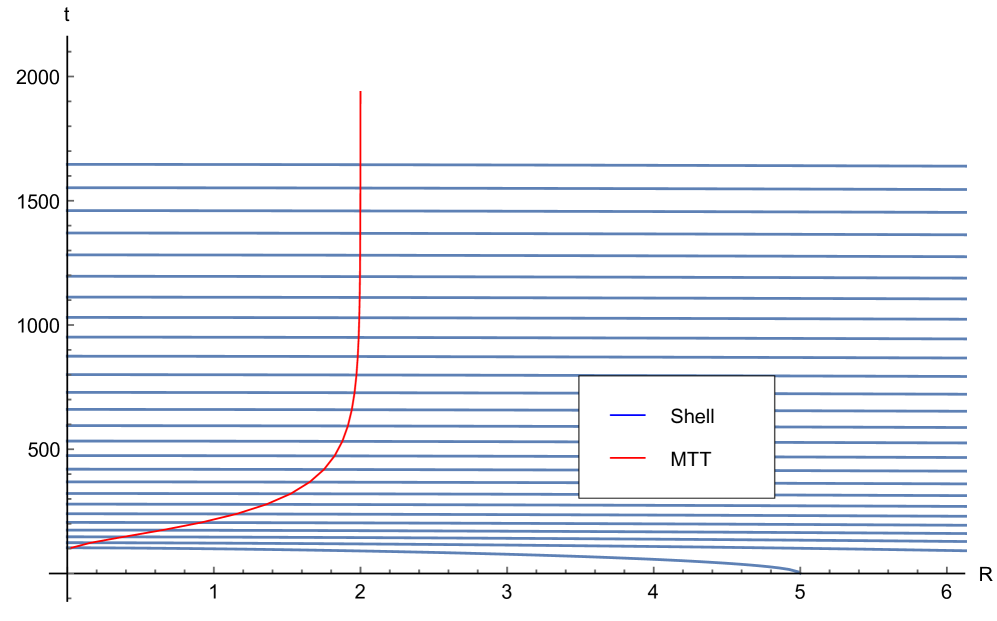
(c)

Figure 9: The graphs show the (a) density distribution, (b) values of $C$, and (c) formation of MTT along with the shells. The MTT begins from the center of the cloud. The straight lines of MTT in (c) represents the isolated horizon phase.

The MTT begins from the central singularity, and develops as a dynamical horizon until at approximately $r=70$, is begins to resemble an isolated horizon. This may also be confirmed from the fact that the density at $r=70$ is almost negligible. However, since the Gaussian profile almost disappears at $r=100$, the $R=2$ is also reached at that value of the shell coordinates. This may be seen from figure 9.

(iv) Two shells falling consecutively on a black hole: Let us assume that a black hole of mass $M$ exists, upon which a density profile of the following form falls:

$$\rho(r)=\frac{8\,(m_{0}/\,r_{0}^{3}\,)\,[(r/r_{0})-\varsigma]^{\,2}}{[2\varsigma+(3+2\varsigma^{2})\sqrt{\pi}e^{\varsigma^{2}}\{1+\operatorname{Erf}(\varsigma)\}]}\,\exp[(2r/r_{0})\varsigma-(r/r_{0})^{\,2}\,],$$ (115)

where $m_{0}=M/2$ is the mass of the shell, $2r_{0}$ is the width of each shell.

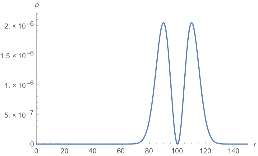
(a)

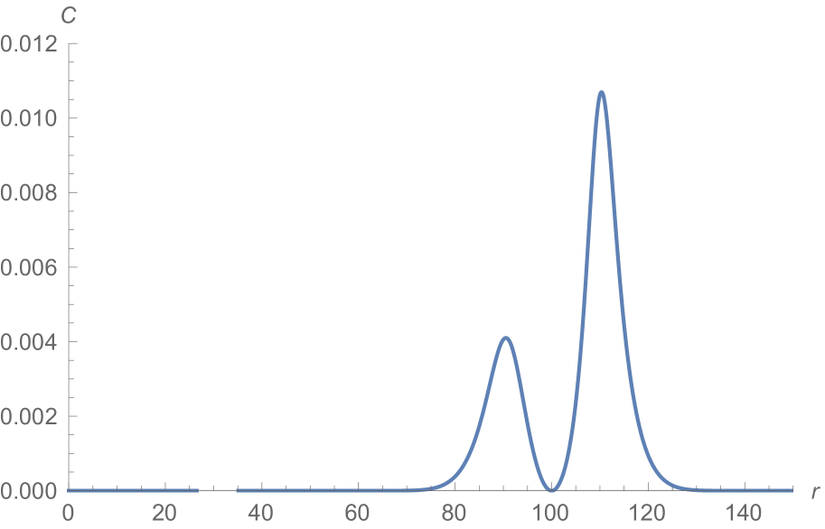
(b)

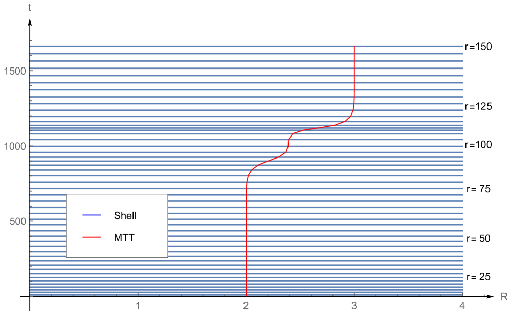
(c)

Figure 10: The graphs show the (a) density distribution, (b) values of $C$, and (c) formation of MTT along with the shells which fall consecutively on a black hole. The MTT begins from $R=2$, where the previous EH is situated. The straight lines of MTT in (c) represents the isolated horizon phase.

If we assume that the initial black hole has the Schwarzschild radius given by $\bar{r}=2M$, then the mass for each shell of radius $r(r>\bar{r})$ is then $m(r)=M+\int_{\bar{r}}^{r}\rho(\hat{r})\hat{r}^{2}\,d\hat{r}$. The quantity $\sigma$ is a parameter which denotes the position where the density vanishes. Here, we have used $M=1$, $r_{0}=10$ and $\varsigma=10$. At around $r=65$, the MTT starts to grow in a spacelike fashion and reaches approximately at $R=2.4$ at approximately $t=1014$ when the $r=100$th shell falls. Note that at this time the $C$ vanishes making the MTT null. This is expected since the density of the shell goes to zero here (see figure 10). Again, just as the next shell starts to fall, the MTT again begins to evolve in a spacelike fashion to reach $R=3$ at $t=1500$ when the shell denoted by $r=140$ has fallen in.

5 Spacetimes admitting viscous matter fields

In this section, we shall consider spacetimes due to collapse of matter whose energy- momentum tensor contains viscous matter fields. The Einstein equations derived in equation (33)-(37) shall be useful in this regard. In the following, we shall derive some general conditions about the nature of the spacetime from these equations. Additionally, it shall also arise that if one assumes some form of equation of state -type relations between some geometric scalar quantities and the density, then the situation simplifies. We shall show below that such relations are indeed possible.

First, note that one may envisage some exact relations involving the the Newman- Penrose scalar $\psi_{2}$ and the Misner- Sharp mass function [82, 83]. The quantity $\psi_{2}$ for this spacetime is given by:

$$\psi_{2} = \frac{e^{-2\beta}}{6}\left[\alpha^{\prime\prime}+{{\alpha}^{\prime}}^{\,2}-\alpha^{\prime}\beta^{\prime}+R^{\prime 2}/R^{2}-R^{\prime\prime}/R+(R^{\prime}\beta^{\prime})/R-(R^{\prime}\alpha^{\prime})/R\right]-\frac{1}{6R^{2}}$$ (116)

$$- \frac{e^{-2\alpha}}{6}\left[\ddot{\beta}+{\dot{\beta}}^{2}-\dot{\alpha}\dot{\beta}+{\dot{R}}^{2}/R^{2}-\ddot{R}/{R}-(\dot{R}\dot{\psi})/R+(\dot{R}\dot{\alpha})/R\right].$$

Using the Einstein equations, above equation (116) can be written in terms of the mass function $F(r,t)$:

$$F(r,t)=\left(\rho+\bar{p}_{t}-\bar{p}_{r}+2\eta\sigma\right)(R^{3}/3)-(\psi_{2}/2)\,R^{3},$$ (117)

where $\bar{p}_{r}=(p_{r}-\zeta\theta)$ and $\bar{p}_{t}=(p_{t}-\zeta\theta)$. The quantity $\mathcal{F}(r,t)=-\psi_{2}\,R^{3}$, has a similar stature as the mass function [82]. The equations similar to those for the mass function $F(r,t)$ given in (3) shall play an important role here and are given by:

$$\dot{\mathcal{F}} = -(1/6)\left[R^{3}\left\{\rho+\bar{p}_{t}+(2/3)\eta\sigma\right\}\right]_{,\,t}-(R^{3}/6)\left[\bar{p}_{r}-(4/3)\eta\sigma\right]_{,\,t}$$ (118)

$$\mathcal{F}^{\prime} = -(1/6)\,R^{3}\rho^{\prime}-(1/6)\left[R^{3}\left(\bar{p}_{t}-\bar{p}_{r}+2\eta\sigma\right)\right]^{\prime}$$ (119)

These two equations may be combined to extract an expression for the time derivative of the density $\dot{\rho}$:

$$\dot{\rho}e^{-\alpha}+\left[\rho+\bar{p}_{r}-(4/3)\eta\sigma\right]\left(\Theta-\sigma\right)=0.$$ (120)

On the other hand, the expression for $\dot{\rho}$ may also be derived from the Bianchi identities, given in the equation (21) and (3), and rewritten as:

$$\dot{\rho} = -\dot{\beta}\left[\rho+\bar{p}_{r}-(4/3)\eta\sigma\right]-(2\dot{R}/R)\left[\rho+\bar{p}_{t}+(2/3)\eta\sigma\right],$$ (121)

$$p_{r}^{\prime} = \left\{(4/3)\eta\sigma\right\}^{\prime}+(2R^{\prime}/R)\left(\bar{p}_{t}-\bar{p}_{r}+2\eta\sigma\right)-\alpha^{\prime}\left\{\rho+\bar{p}_{r}-(4/3)\eta\sigma\right\}.$$ (122)

Using the Bianchi identity (121) into the equation (120), we have a relation involving the matter variables and the geometric variables given by:

$$\left(\rho+\bar{p}_{r}\right)=\frac{8}{3}\eta\sigma-\frac{4}{3}\eta\theta+e^{-\alpha}\,\frac{2\dot{R}}{R\sigma}\left(\bar{p}_{t}-\bar{p}_{r}\right).$$ (123)

This equation gives some crucial input regarding the pressure anisotropy $\left(\bar{p}_{t}-\bar{p}_{r}\right)$ and its relation to the shear scalar $\sigma$. The pressure anisotropy must be interpreted as the generator of the shear scalar and hence must be proportional to it. Indeed, using the equation (123) in (121), we have:

$$\dot{\rho}=\frac{6\dot{R}^{2}}{R^{2}}e^{-\alpha}\left[2\eta+\frac{\bar{p}_{t}-\bar{p}_{r}}{\sigma}\right],$$ (124)

which makes our claim, that pressure anisotropy must lead to shear, explicit. However, we shall show below that the claim still holds even if we assume the matter density to be spatially uniform throughout the collapsing cloud. We must point out that such an assumption is not contradictory to the presence of shear or pressure anisotropy. We shall elaborate on this issue below as well as in the following sections when we take specific examples. To show this, we first derive another expression for the time change of density which involves the radial pressure only. If the density is uniform, simple integration of equations (119) implies that $\mathcal{F}(r,t)=-(R^{3}/6)\left(\bar{p}_{t}-\bar{p}_{r}+2\eta\sigma\right)$. Using this in (118) we have

$$\dot{\rho}=-(3\dot{R}/R)\left[\rho+\bar{p}_{r}-(4/3)\eta\sigma\right].$$ (125)

Now, let us rewrite the Binachi identity (121), using the equations (15) which gives us:

$$\left(\rho+\bar{p}_{r}\right)\theta=-\dot{\rho}e^{-\alpha}-\frac{2\dot{R}}{R}\left(\bar{p}_{t}-\bar{p}_{r}\right)e^{-\alpha}+\frac{4}{3}\eta\sigma^{2},$$ (126)

which may also be written in the following form, equivalent to (124):

$$\dot{\rho}e^{-\alpha}=\left[(4/3)\eta\sigma^{2}-\left(\rho+\bar{p}_{r}\right)\Theta\right]\left[1-\frac{(2/3)\left(\bar{p}_{t}-\bar{p}_{r}\right)}{\rho+\bar{p}_{r}-(4/3)\eta\sigma}\right]^{-1}.$$ (127)

The radial derivative of the equation (126) along with (127), gives the following equation:

$$\left(\rho+\bar{p}_{r}\right)\theta^{\,\prime}+\left(\rho+\bar{p}_{r}\right)^{\,\prime}\theta = \left(\dot{\rho}e^{-\alpha}\right)^{\prime}\left[1+\frac{(2/3)\left(\bar{p}_{t}-\bar{p}_{r}\right)}{\rho+\bar{p}_{r}-(4/3)\eta\sigma}\right]+\left[(4/3)\eta\sigma^{2}\right]^{\,\prime}$$ (128)

$$\,\,~{}~{}~{}~{}~{}~{}~{}~{}-\dot{\rho}e^{-\alpha}\left[\frac{(2/3)\left(\bar{p}_{t}-\bar{p}_{r}\right)}{\left(\rho+\bar{p}_{r}-(4/3)\eta\sigma\right)}\right]^{\prime},$$

which along with the radial part of Bianchi identity (122) give the following elaborate form:

$$\left(\rho+\bar{p}_{r}\right)\theta^{\,\prime} =-\left[(4/3)\eta\sigma^{\prime}-(4/3)\eta\sigma\,\alpha^{{}^{\prime}}+(2R^{{}^{\prime}}/R)\left(\bar{p}_{t}-\bar{p}_{r}+2\eta\sigma\right)\right]{\theta}$$ (129)

$$+\left[\frac{(2/3)}{\left(\rho+\bar{p}_{r}-(4/3)\eta\sigma\right)-\frac{2}{3}\left(\bar{p}_{t}-\bar{p}_{r}\right)}\right]\left[\alpha^{{}^{\prime}}\left(\rho+\bar{p}_{r}\right)\{2\eta\sigma^{2}-\bar{p}_{t}\theta\left(\bar{p}_{t}-\bar{p}_{r}\right)\}\right.$$

$$~{}~{}~{}~{}~{}~{}~{}\left.+\left\{(\rho+\bar{p}_{r})\Theta+(4/3)\eta\sigma^{2}\right\}\left\{\left(\bar{p}_{t}-\bar{p}_{r}\right)^{{}^{\prime}}-\frac{2\left(\bar{p}_{t}-\bar{p}_{r}\right)^{2}}{\left(\rho+\bar{p}_{r}-4/3\cdot\eta\sigma\right)}\right.\right.$$

$$~{}~{}~{}~{}~{}~{}~{}~{}~{}~{}~{}~{}~{}~{}\left.\left.-\frac{4\eta\sigma\left(\bar{p}_{t}-\bar{p}_{r}\right)}{\left(\rho+\bar{p}_{r}-4/3\cdot\eta\sigma\right)}\right\}-8/3\cdot\alpha^{\prime}\eta^{2}\sigma^{3}\right]+\left\{(4/3)\eta\sigma^{2}\right\}^{\prime}.$$

Several results follow directly from equation (129). Let the pressure anisotropy $(p_{t}-p_{r})$, and the viscosity parameters $\eta$ and $\zeta$ vanish. If we write $p_{r}=p_{t}\equiv p$, then the above equation reduces to:

$$\left(\rho+p\right)\theta^{\,\prime}=0.$$ (130)

This implies that for the gravitational collapse of uniform density perfect fluid with irrotational motion, the expansion scalar must be spatially uniform. Furthermore, the spacetime must be isotropic as well as conformally flat [83, 84, 85]. These results hold true even if the spacetime has bulk viscosity but negligible shear viscosity [83]. However, if the fluid is dissipative, with non- vanishing shear viscosity, these results donot hold and expansion becomes a scalar function. The situation however alters significantly if the pressure anisotropy arising through $(p_{t}-p_{r})$ is also taken into account. As may be seen from the equation (129), these anisotropies are in the same footing as the shear terms. Indeed, then one may envisage situations where the quantities arising from the dissipative forces like the shear and bulk viscosity cancel those due to anisotropy, leading to spatially uniform expansion scalar, just like for perfect fluids. Although that situation would be highly fine tuned, it is not unlikely. To summarise, we have shown that if the fluid has shear and bulk viscosity, as well as pressure anisotropy, then generically the spacetime will not admit isotropy, conformal flatness or spatially uniform expansion scalar.

This brings into question the possibility if the local anisotropy of fluids may be identified as the source of viscous effects. Given the form of these quantities in (123), (124) and in (129), this expectation holds ground. In the following, we shall assume that relation of this kind do exist, and to give form to this expectation, we assume simple linear relation among these quantities, like $(p_{t}-p_{r})\propto\sigma$. To put it on a firmer perspective, they are to be related to the density function through the following constraints: $p_{t}=k_{t}\rho$, $\sigma=k_{\sigma}\rho$, and $\theta=k_{\theta}\rho$. The values of the constants $k_{t},k_{\sigma}$ and $k_{\theta}$ shall be chosen in such a way that the spacetime preserves the spherical symmetry and that any deviation due to shear will be negligible.

5.1 Time independent mass function

To study a realistic collapse phenomena, pressure and viscosity contributions to energy momentum tensor of the collapsing cloud must be included. To begin with, let us assume that the collapsing cloud has a certain fixed radial pressure, given by $p_{r}=(4/3)\eta\sigma+\zeta\theta$. This particular combination is chosen so that the viscosity terms in the equation of motion cancel the effects of radial pressure during the collapse. This choice also keeps continuity with the study of pressureless collapse carried out in the previous sections. However, to retain the physical importance of our model, we continue to retain the combination $[p_{t}+(2/3)\eta\sigma-\zeta\theta]$ to be non- zero. This particular term includes tangential part of the pressure along with certain viscosity terms. The reasons for these choices is only mathematical simplicity. Also, as we shall see, this choice gives us a time independent Misner-Sharp mass function.

The set of the Einstein equations for gravitational collapse of matter cloud which satisfies these conditions are given by:

$$F^{\prime} = \rho\,R^{\prime}\,R^{2}$$ (131)

$$\dot{F} = -(R^{2}\dot{R})\,({p}_{r}+\frac{4}{3}\eta\sigma-\zeta\theta)=0,$$ (132)

$$\alpha^{\prime} = (2R^{\prime}/\rho R)\left[p_{t}+(2/3)\eta\sigma-\zeta\theta\right],$$ (133)

$$(\dot{G}/{G}) = 2\alpha^{\prime}(\dot{R}/R^{\prime}),$$ (134)

$$F(r,t) = R(r,t)(1-G+H),$$ (135)

where $H(r,t)=e^{-2\alpha(r,t)}\dot{R}^{2}$ and $G(r,t)=e^{-2\beta(r,t)}R^{\prime 2}$. The number of unknowns to be determined here are more than the independent Einstein equations (132)-(135), we close the system with the constraints $p_{t}=k_{t}\rho$, $\sigma=k_{\sigma}\rho$, and $\theta=k_{\theta}\rho$ given above.

Using these equations of state, solutions of the Einstein equations (133) and (134) become

$$\exp(\,2\alpha)=R^{\,4a_{1}},\hskip 28.45274pt\exp(\,2\beta)=\frac{R^{\prime 2}}{b(r)R^{\,4a_{1}}},$$ (136)

where we have introduced the constants $a_{1}=k_{t}+(2/3)\eta k_{\sigma}-\zeta k_{\theta}$. Using these redefinitions, the line element (33) may be rewritten as:

$$ds^{2}=-R^{\,4a_{1}}dt^{2}+\frac{R^{\prime 2}}{b(r)R^{\,4a_{1}}}dr^{2}+R(r,t)^{2}d\theta^{2}+R(r,t)^{2}\sin^{2}{\theta}\,d\phi^{2}$$ (137)

The equation of motion (135) is also simplified to have the following form:

$$\dot{R}=-R^{2a}\left[\frac{F(r)}{R}-1+b(r)R^{\,4a_{1}}\right]^{1/2}.$$ (138)

To study evolution of the horizon and the outgoing null geodesics (and the event horizon), and to simplify the solutions of the equation of motion (135), we choose the parameter to be $a_{1}=-(1/4)$. This choice simplifies the solution of the equation of motion (135), and the time curve of the collapsing shell is given by

$$dt = -\frac{R\,dR}{[F(r)+b(r)-R(r,t)]^{1/2}}.$$ (139)

To solve the integral, we choose a parametric form to relate the functions $R(r,t)$, $F(r)$ and $b(r)$. A particular simple choice is given as

$$R=(F/b)\cos^{2}\left(\eta/2\right).$$ (140)

Using this form, the equation of collapse simplifies and the time curve is obtained from the equation:

$$dt=\left(\frac{F^{2}}{2b^{2}}\right)\frac{\sin\eta\,\cos^{2}(\eta/2)}{[F+b-(F/b)\cos^{2}(\eta/2)]^{1/2}}\,\,d\eta.$$ (141)

The solution of this equation is the time curve of the collapsing shell and is given by

$$t = \frac{4}{3}[F+b-(F/b)\cos^{2}(\eta/2)]^{1/2}\left[F+b+(F/2b)\cos^{2}(\eta/2)\right]$$ (142)

$$~{}~{}~{}~{}~{}~{}~{}~{}~{}~{}~{}~{}~{}~{}~{}~{}~{}~{}~{}~{}~{}~{}-(4/3)\{F+b-(F/b)\}^{1/2}\left[F+b+(F/2b)\right].$$

The boundary conditions are chosen such that the collapse begins at $\eta=0$ and reaches the central singularity at $\eta=\pi$. At the beginning of the collapse, $\eta=0$ we have $R(t_{i},r)=[F(r)/b(r)]$ with $t_{i}=0$. At the end state of the collapse process when $\eta=\pi$, we naturally have $R=0$. Note that the time of formation of central singularity, or the time the shell reaches singularity, is also obtained from the above equation:

$$t_{s}=\frac{4}{3}\left[\left(F+b\right)^{\frac{3}{2}}-\{F+b-(F/b)\}^{1/2}\left\{F+b+(F/2b)\right\}\right].$$ (143)

From these equations, it is also possible to track the formation of apparent horizon and determine the exact time the shell reaches it’s Schwarzschild radius. However, for the present purposes, we shall utilize the numerical techniques from the previous sections to track the formation of the MTTs, determine its signature and eventually note how the cloud settles down to the null isolated horizon.

The dynamics of the marginally trapped surfaces (whether they are timelike, spacelike or null) depends upon the sign of the expansion parameter $C$ defined in equation (6). We take the timelike vector field to be $u^{\mu}=\chi l^{\mu}+(2\chi)^{-1}n^{\nu}$ and the spacelike vector field to be $x^{\mu}=\chi l^{\mu}-(2\chi)^{-1}n^{\nu}$.

$$T_{\mu\nu}l^{\mu}l^{\nu} = (1/4\chi)\left[\rho+p_{t}-(4/3)\eta\sigma-\zeta\theta+\left(p_{t}-p_{r}\right)\right],$$ (144)

$$T_{\mu\nu}l^{\mu}n^{\nu} = (1/2)\left[\rho-\left(p_{t}-(4/3)\eta\sigma-\zeta\theta+\left(p_{t}-p_{r}\right)\right)\right].$$ (145)

Using $p_{r}=(4/3)\eta\sigma+\zeta\theta$, the equations lead to the following form of $C$:

$$C = (1/2\chi)\left[\frac{\rho+2\left\{p_{t}-(4/3)\eta\sigma-\zeta\theta\right\}}{4\pi/\mathcal{A}-(1/2)\left[\rho-2\left\{p_{t}-(4/3)\eta\sigma-\zeta\theta\right\}\right]}\right].$$ (146)

Examples

(i) Let us consider a Gaussian profile. The density profile is same as before and is given by:

$$\rho(r)=\frac{m_{0}}{\pi^{3/2}r_{0}^{3}}\exp(-r^{2}/r_{0}^{2}),$$ (147)

where $m_{0}$ is the total mass of the matter cloud, $r_{0}$ is a parameter which indicates the distance where the density of the cloud decreases to $[\rho\,(0)/e]$.

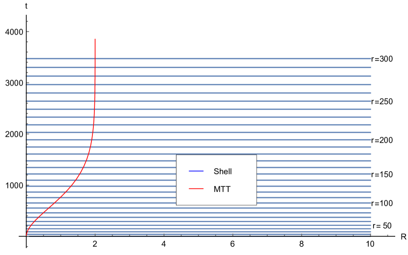
(a)

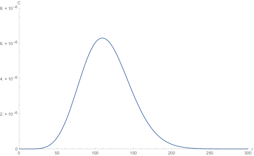
(b)

Figure 11: The graphs show the (a) formation of MTT along with the shells, (b) values of $C$. The MTT begins from the center of the cloud and remains spacelike. The straight lines of MTT in (a), after the shell at $r=250$, represents the isolated horizon phase.

Just as before, we choose $r_{0}=100\,m_{0}$. Here also, the MTT begins from the central singularity, and develops as a dynamical horizon until it approaches the isolated horizon at approximately $r=200$. This may also be confirmed from the fact that the density at $r=200$ is almost negligible. The density profile almost disappears at $r=380$, and beginning at that value of shell coordinate, the MTT remains at $R=2$. The nature of the formation of singularity is identical to the LTB case discussed in the previous sections. However the difference is now with respect to the time at which the MTT forms. For the LTB, the shell at $r=200$ forms the MTT at $t=3215$, whereas for the same choice of the density parameters, but with the choice of the parameter $a_{1}=-(1/4)$, the same shell forms the MTT at $t=1912$. The reason is that for these choices, the $p_{r}$ is now non- zero and hence contributes to faster formation of the MTT (see figure 11). There also exists contributions from the $p_{t}$ terms to the proper time of the observer falling along the shell.

(ii) For the density profile given by the following form,

$$\rho(r)=\frac{m_{0}}{8\pi r_{0}^{3}}\exp(-r/r_{0}),$$ (148)

the situation is identical to the above case for the Gaussian profile.

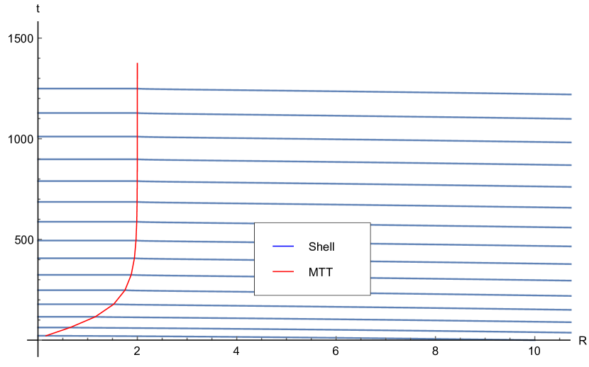
(a)

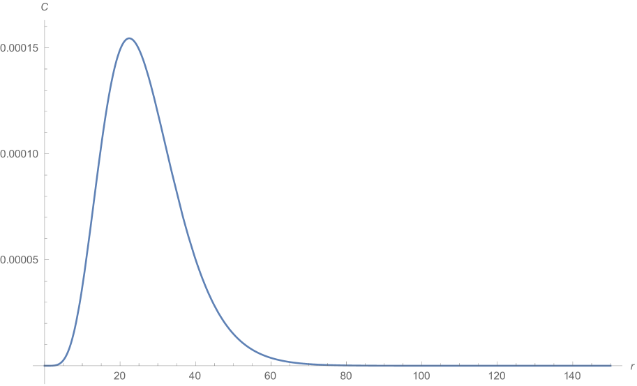
(b)

Figure 12: The formation of MTT (a), and (b) values of $C$.

The time of formation of the MTT is lower than that obtained for the LTB case. For the LTB collapse, the MTT begins from the central singularity, and develops as a dynamical horizon until at approximately $r=70$, is begins to resemble an isolated horizon. Here, the MTT formation and it’s spacelike nature is retained although the time of formation of the isolated horizon is lowered at $t=406$ from that in the LTB case which happens at $t=660$ (see figure 12).

5.2 Time dependent mass function

Let us consider the system in it’s full generality. The Einstein equations shall have all following terms:

$$\rho = \frac{F^{\prime}}{R^{2}R^{\prime}};\hskip 14.22636pt{p}_{r}=-\frac{\dot{F}}{R^{2}\dot{R}}+(4/3)\eta\sigma+\zeta\theta$$ (149)

$$\alpha^{\prime} = \frac{2R^{\prime}}{R}\frac{p_{t}-p_{r}+2\eta\sigma}{\rho+p_{r}-(4/3)\eta\sigma-\zeta\theta}-\frac{{p}_{r}^{\prime}-(4/3)\eta\sigma^{\prime}-\zeta\theta^{\prime}}{\rho+p_{r}-\frac{4}{3}\eta\sigma-\zeta\theta}$$ (150)

$$(\dot{G}/G) = (2\alpha^{\prime})(\dot{R}/R^{\prime})\,;\,\hskip 14.22636ptF(r,t)=R(1-G+H).$$ (151)

Note that due to our generality, the Misner- Sharp mass function shall acquire time dependence. To solve this set of highly nonlinear coupled equations, we assume a set of constraints on the dynamical quantities: $p_{r}=k_{r}\rho$, $p_{t}=k_{t}\rho$, $\sigma=k_{\sigma}\rho$ and $\theta=k_{\theta}\rho$. By using these conditions, the solutions of metric functions are

$$\exp(2\alpha)=\frac{R^{\,4a_{1}}}{\rho^{\,2a_{2}}},\hskip 28.45274pt\exp(2\beta)=\frac{R^{\prime}{}^{2}}{1+r^{2}B(r,t)},$$ (152)

where the parameters $a_{1}$ and $a_{2}$ are defined as $a_{1}=[k_{t}-k_{r}+2\eta k_{\sigma}]/[1+k_{r}-(4/3)\eta k_{\sigma}-\zeta k_{\theta}]$ and $a_{2}=[k_{r}-(4/3)\eta k_{\sigma}-\zeta k_{\theta}]/[1+k_{r}-(4/3)\eta k_{\sigma}-\zeta k_{\theta}]$. The line element for this spacetime may thus be written as:

$$ds^{2}=-\frac{R(r,t)^{4a_{1}}}{\rho(r,t)^{2a_{2}}}dt^{2}+\frac{R(r,t)^{\prime 2}}{1+r^{2}B(r,t)}dr^{2}+R(r,t)^{2}\,[\,d\theta^{2}+\sin^{2}{\theta}\,d\phi^{2}]$$ (153)

The equation of motion obtained from the equation (151) is reduced to the form:

$$\dot{R}=-R^{\,2a_{1}}\rho^{\,-a{{}_{2}}}\left[\frac{F(r,t)}{R}+r^{2}B(r,t)\right]^{1/2}.$$ (154)

For exact analytical solution, we introduce simplifications. Let us assume that the mass function $F(r,t)$, the metric function $B(r,t)$ and the density $\rho(r,t)$ are of the separable type:

$$F(r,t)=F_{1}(r)F_{2}(t),\,\,~{}~{}B(r,t)=B_{1}(r)B_{2}(t),\,\,~{}~{}\rho(r,t)=\rho_{1}(r)\rho_{2}(t),$$ (155)

where some of these functions are related, with the following conditions: $B_{1}(r)=k(r)/r^{2}$, $B_{2}(t)=-F_{2}(t)=-\rho_{2}(t)^{2a_{2}}$. Now, with the choice of the parametric form of $R(r,t)$, given by

$$R=[F_{1}(r)/k(r)]\,\cos^{2}\,(\eta/2),$$ (156)

the equation of motion of the collapsing cloud (154), gives the following time curve:

$$dt=\frac{[F_{1}(r)\,\cos^{2}(\eta/2)]^{(1-2a_{1})}\,\rho_{1}^{\,a_{2}}}{k(r)^{(3/2-2a_{1})}}\,d\eta.$$ (157)

The solution of this equation which determines motion of the collapsing cloud is given by complicated relations involving the Hypergeometric functions

$$t_{{shell}} = \frac{2F_{1}(r)^{1-2a_{1}}\rho_{1}(r)^{a_{2}}\cos(\eta/2)^{3-4a_{1}}}{(4a_{1}-3)k(r)^{3/2-2a_{1}}}\,\,{}_{2}F_{1}\left[\frac{1}{2},\frac{3}{2}-2a_{1};\frac{5}{2}-2a_{1};\cos^{2}(\eta/2)\right]$$ (158)

$$~{}~{}~{}~{}~{}~{}~{}~{}~{}~{}~{}~{}~{}~{}~{}~{}~{}~{}~{}~{}~{}~{}~{}~{}~{}~{}~{}~{}~{}-\frac{2\sqrt{\pi}F_{1}(r)^{1-2a_{1}}\rho_{1}(r)^{a_{2}}}{(4a_{1}-3)k(r)^{3/2-2a_{1}}}\frac{\Gamma[5/2-2a_{1}]}{\Gamma[2-2a_{1}]},$$

where ${}_{2}F_{1}(a,b;c;z)$ is the Gauss Hypergeometric function, and $\Gamma(x)$ is the Gamma function. The boundary conditions are chosen such that collapse starts at $\eta=0$, where $R(t_{i},r)=[F(r)/k(r)]$ and $t=0$. The cloud reaches the central singularity at $\eta=\pi$ where $R=0$. In the $t$- coordinates, the time of formation of central singularity is

$$t_{s}=\frac{2\sqrt{\pi}F_{1}(r)^{1-2a_{1}}\rho_{1}(r)^{a_{2}}}{(3-4a_{1})k(r)^{3/2-2a_{1}}}\frac{\Gamma[5/2-2a_{1}]}{\Gamma[2-2a_{1}]}.$$ (159)

The dynamics of the marginally trapped surfaces (whether they are timelike, spacelike or null) depends upon the sign of the expansion parameter $C$, and is given by:

$$C = \frac{1}{2\chi}\left[\frac{\rho+p_{t}-(4/3)\eta\sigma-\zeta\theta+\left(p_{t}-p_{r}\right)}{(4\pi/\mathcal{A})-(1/2)\{\rho-\{p_{t}-(4/3)\eta\sigma-\zeta\theta+\left(p_{t}-p_{r}\right)\}\}}\right].$$ (160)

Examples

(i) Gaussian: The radial pressure has decreased, and hence the time of formation of singularity or the MTT is at a larger time (see figure 13).

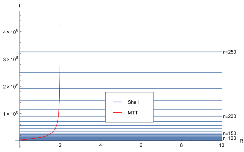
(a)

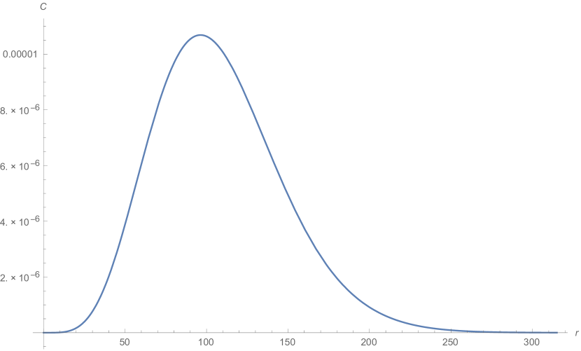
(b)

Figure 13: The graphs show the (a) formation of MTT along with the shells, (b) values of $C$. Again, note that the MTT begins from the center of the cloud and remains spacelike until it reaches the isolated horizon phase.

The MTT is still spacelike. $k_{r}=(1/2)$, $k_{t}=1/4$, $\eta=1/16$, $k_{\sigma}=1/4$, $\zeta=(1/2)$, $k_{\theta}=(3/2)$, giving $a_{1}=-0.3$ and $a_{2}=-0.37$. Notice that for $r=200$, which for the LTB case reached the isolated horizon at $t=3215$, here it happens at $t=9\times 10^{7}$, which is approximately $10^{3}$ factor higher. The reason is that with the choice of a time dependent $F(r,t)$, the radial pressure has decreased considerably and hence, the time of formation of the MTT for each shell also goes up. The nature of formation of MTT however remains identical.

(ii) Large shell: The nature of formation of MTT here is drastically different in nature from that described in the previous examples. Here, we observe formation of timelike MTTs.

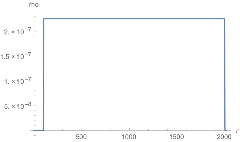
(a)

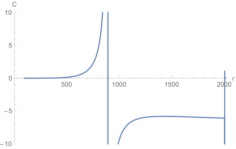
(b)

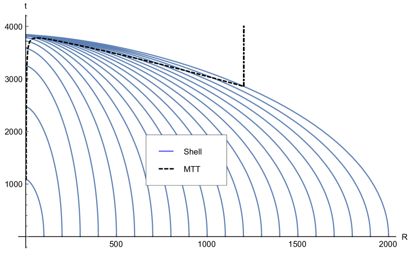
(c)

Figure 14: The graphs show the (a) formation of MTT along with the shells, (b) values of $C$. The MTT is timelike. It first forms at $t=3000$ approximately, and bifurcates in one direction to reach the IH and in another direction to match with the DH evolving from the previous black hole.

Here, for a more complicated collapse dynamics, the density profile generate a timelike tube. The MTT forms at about $r=1800$ and bifurcates to reach the initial black holes. The timelike nature of the MTT is also confirmed from the values of $C$ (figure 14). Here $k_{r}=(1/80)$, $k_{t}=1/81$, $\eta=1/16$, $k_{\sigma}=1/20$, $\zeta=(1/12)$, $k_{\theta}=(1/8)$, giving $a_{1}=0.006$ and $a_{2}=-0.002$.

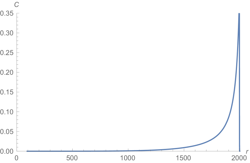
(a)

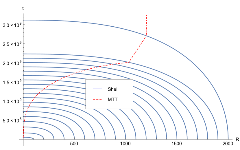
(b)

Figure 15: The graphs are for the density profile of figure 14, but with different parameters. Here, the MTT is spacelike.

However, if the following choice of parameters is made, the MTT is spacelike: $k_{r}=1/2$, $k_{t}=1/10$, $\eta=1/8$, $k_{\sigma}=1/4$, $\zeta=1/2$, $k_{\theta}=3/2$, with $a_{1}=-0.48$ and $a_{2}=-0.41$ (see figure 15).

(iii) Two consecutive shells falling on a black hole: Here $k_{r}=(1/80)$, $k_{t}=1/81$, $\eta=1/16$, $k_{\sigma}=1/20$, $\zeta=(1/12)$, $k_{\theta}=(1/8)$, giving $a_{1}=0.006$ and $a_{2}=-0.002$ (see figure 16).

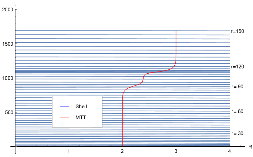
(a)

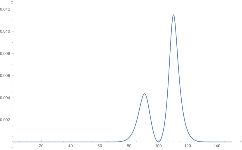
(b)

Figure 16: The graphs show the (a) formation of MTT along with the shells, (b) values of $C$. The MTT begins from the center of the cloud and remains spacelike. The straight lines of MTT in (a) represents the isolated horizon phase.

The nature of formation of MTT is identical to that described for the LTB model although the time of formation of the MTT is not delayed for these choice of parameter fields.

6 Discussions

In this paper, we have developed analytical and numerical techniques to study gravitational collapse of a large class of matter fields in Einstein’s theory. The main focus was to obtain the trapped regions and locate the marginally trapped surfaces for some general class of energy- momentum tensors, including fluids admitting bulk and shear viscosity. For the purpose of generality, we have included the homogeneous as well as inhomogeneous dust models. While the dust models have been studied earlier [3], the detail study of the formation and time- development of the EH and the MTTs for a generic class of energy- momentum tensors, through analytical as well as numerical means, to our knowledge, have not been carried out in the literature. Our analytical methods focus on two specific aspects. (see however, [44, 54, 72]). The first aspect is to use the equations of gravitational collapse in the $R(r,t)-t$ coordinate system, to trace the formation of the EH and the MTTs, simultaneously with the collapse of the matter cloud. The use of the $R(r,t)$ is specially advantageous, since it is possible to track the horizons as well as the collapsing sphere at each moment. The second aspect is the development of numerical codes to locate trapped regions and marginally trapped surfaces for each of these matter fields. Through these numerical techniques, we have ascertained the validity of the analytical calculations as well as obtained a faithful representation of the general expectations during gravitational collapse. In particular, we have obtained the signature of the MTTs during each of the collapse scenarios and a general conclusion may be reached: The MTTs in the OSD models are timelike. The situation for LTB- like collapse is more complicated. Here, for generically for $\dot{m}(r)>0$, the MTTs are spacelike and hence, are all MTTs are dynamical horizons and reach the isolated horizon phase in equilibrium. Some variations are however observed, although the effects are most likely unobservable to the observer outside the black hole. Thus, although the results are valid for spherical symmetric spacetimes, some general conclusions may possibly be drawn about the behavior of MTTs during the collapse.

While dealing with the viscous fluid, we have however kept the shear coefficient low so that the spacetime does not deviate drastically from spherically symmetry. These parameter ranges, of the coefficients arising in the energy- momentum tensor, have been utilised to numerically study the evolution of the MTTs in these cases. Out of this parameter ranges, we have further restricted to a smaller set of initial data so that we do not encounter shell- crossing during gravitational collapse or have trapped surfaces at the beginning of the process. We observe that, within a particular set of assumptions used here, it is possible to exploit the freedom of choice of equation of state and the viscosity parameters to manipulate the nature as well as time of formation of the MTT. Indeed, in the previous section, we have shown through examples, that alternate choices of initial data may lead to MTTs which are either timelike or spacelike. Furthermore, these choices also alter the time of formation of MTTs compared to the dust models, in the sense that MTT formation may be delayed or accelerated, compared to the dust models, by suitable choices in the fluid parameters. We believe that the results obtained in this paper may help in forming a general outlook about the time development of Marginally Trapped Surfaces during gravitational collapse.

An important aspect of study of the MTTs or trapped surfaces involve identifying boundary of a black hole region. The boundary of a trapped region is not known, although the Eardley conjecture claims that the event horizon of a black hole spacetime may be thought of as the boundary of (marginally outer) trapped surfaces [86]. Indeed, it has been shown that for Vaidya- type null collapse scenarios with mass $m(v)$ having upper bound, and accreting mass such that $\dot{m}(v)\geq 0$, the conjecture holds [87]. However interestingly, it has also been found that given a trapping horizon, trapped surfaces (or parts of it) may extend outside of the horizon, and into the initial flat region of the Vaidya- spacetime, and furthermore non-spherically symmetric trapped surfaces may also extend outside the standard spherically symmetric trapping horizon [74, 75, 80]. So, the exact boundary of a trapped region is not clearly specifiable as of now. A related question is then the following: if the Eardley conjecture holds, does the event horizon allow a local description? One should expect from the global nature of the EH that this should not be so. Again for Vaidya- type collapse processes, it has been shown that trapped surfaces may be constructed which extend into the future and hence acquires non- local nature. Thus, the location and nature of the boundary of a strictly trapped region remains unknown. It seems that the process of further development needs numerical study of MTTs in GR as well as in other alternate gravity theories to gain insight into the properties of MTTs. These issues will be addressed in future studies.

Appendix: Junction Conditions

The Israel- Darmois junction conditions provide a set of rules and boundary conditions which has been used in the previous sections. These boundary conditions are summarized below for some simple cases. In the following, we provide the junction conditions for a simple model: a $K=0$ OSD model as the interior spacetime joined to an exterior Schwarzschild spacetime (denoted by $\mathcal{M^{-}}$) of mass $M$ (denoted by $\mathcal{M^{+}}$), along a spacelike hypersurface $\Sigma$. Let us denote the coordinates on this surface to be $(\tau,\theta,\phi)$. From $\mathcal{M^{-}}$, we can write down the surface $\Sigma$ as $f_{-}(r,t)=r-r_{b}=0$, and hence, the induced metric on $\Sigma$ is

$$ds^{2}_{-}=a(\tau)^{2}\left(-d\tau^{2}+r_{b}^{2}\,d\Omega^{2}\,\right).$$ (161)

Note that the coordinates $t$ and $\tau$ are related through the relation $dt/d\tau=a(\tau)$. From the point of view of the exterior spacetime, the hypersurface may be described by $r=R(\tau)$ and $t=T(\tau)$, with no change in the angular variables. The line element of the exterior manifold is then given by

$$ds^{2}_{+}=-\left(Z\dot{T}^{2}-Z^{-1}\dot{R}^{2}\right)d\tau^{2}+R(\tau)^{2}\left(d\theta^{2}+\sin^{2}{\theta}d\phi\right)$$ (162)

where $Z=\left(1-2M/R\right)$. The matching of the metric immediately implies that the following two conditions hold:

$$R(\tau)=r_{b}\,a(\tau)\,;~{}~{}~{}~{}a(\tau)^{\,2}=\left[Z\left(dT/d\tau\right)^{2}-Z^{-1}\left(dR/d\tau\right)^{2}\right].$$ (163)

The normal vector field $n^{a}$ for $\mathcal{M^{-}}$ and the external spacetime $\mathcal{M^{+}}$ are given respectively by:

$$n_{a}=a(\tau)\,(dr)_{a},~{}~{}~{}~{}~{}n_{a}=-(dR/d\tau)\,(d\tau)_{a}+(dT/d\tau)\,(dr)_{a}.$$ (164)

The velocity of observer on the cloud is also determined for these two patches of spacetime separately and are given by:

$$\frac{dR(r_{b},\tau)}{d\tau}=-a(\tau)\left[F(r_{b})/R\right]^{\,1/2},$$ (165)

where the $-$ve sign is chosen to signify collapse. The velocity as observed from the external coordinates is then:

$$\frac{dR}{dT}=-\left(2M/R\right)\left(1-2M/R\right).$$ (166)

Note also that the second of the metric matching condition, along with the equation (165) implies that

$$\left(\frac{dT}{d\tau}\right)=a/(1-2M/R)$$ (167)

Using the normal vector fields, the extrinsic curvatures of the interior and the exterior spacetime may also be determined, and they give:

$$K^{-}_{\tau\tau} = 0,$$ (168)

$$K^{+}_{\tau\tau} = -\sqrt{\frac{2M}{R}}\left(1-\frac{2M}{R}\right)\ddot{T}+\dot{a}\sqrt{\frac{2M}{R}}+\frac{4M^{2}a^{2}}{\left(1-\frac{2M}{R}\right)r_{s}^{3}},$$ (169)

$$K^{-}_{\theta\theta} = R\left[1-\frac{F}{R}+\frac{2M}{R}\right]^{1/2},~{}~{}~{}~{}K^{+}_{\theta\theta}=R.$$ (170)

The $K_{\tau\tau}$ matching gives us the equation (167). The $K_{\theta\theta}$ matching gives us the equation:

$$F(r_{b})\equiv m\,r_{b}^{3}=2M.$$ (171)

A similar exercise may also be carried out to join the interior spacetime created due to viscous fluid collapse, given by equation (153), with the external Schwarzschild spacetime. In that case, the matching gives the following set of conditions. First, the $K_{\theta\theta}$ matching again gives

$$F(r_{b},\tau)\equiv m(r_{b},\tau)\,r_{b}^{3}=2M,$$ (172)

This matching, along with the condition from (27), leads to the following relation involving the radial pressure and viscosity terms at the boundary

$$p_{r}=\zeta\theta+\,(4/3)\eta\,\sigma.$$ (173)

References

- [1] S.W. Hawking and G.F.R. Ellis, The Large Scale Structure of Spacetime, Cambridge University Press, Cambridge 1975.
- [2] Robert M. Wald, General Relativity, University of Chicago Press, 1984.
- [3] L.D. Landau and E.M. Lifshitz, The Classical Theory of Fields, Pergamon Press, 1975.
- [4] P.S. Joshi, Gravitational Collapse and Spacetime Singularities, Cambridge University Press, Cambridge, 2007.
- [5] R. Penrose, Phys. Rev. Lett. 14, 57 (1965).
- [6] R. Penrose, Riv. Nuovo Cim. 1, 252 (1969) [Gen. Rel. Grav. 34, 1141 (2002)].
- [7] S. Datt, Zs. f. Phys. 108, 314 (1938).
- [8] J. R. Oppenheimer and H. Snyder, Phys. Rev. 56, 455 (1939).
- [9] G. Lemaitre, Gen. Rel. Grav. 29, 641 (1997).
- [10] R. C. Tolman, Proc. Nat. Acad. Sci. 20, 169 (1934) [Gen. Rel. Grav. 29, 935 (1997)].
- [11] H. Bondi, Mon. Not. Roy. Astron. Soc. 107, 410 (1947).
- [12] C. W. Misner and D. H. Sharp, Phys. Rev. 136, B571 (1964).
- [13] W. C. Hernandez and C. W. Misner, Astrophys. J. 143, 452 (1966).
- [14] P. S. Joshi and D. Malafarina, Int. J. Mod. Phys. D 20, 2641 (2011).
- [15] D. M. Eardley and L. Smarr, Phys. Rev. D 19, 2239 (1979).
- [16] D. Christodoulou, Commun. Math. Phys., 93, 171 (1984).
- [17] A. Papapetrou, ‘Formation of a singularity and causality’. In A Random Walk in Relativity and Cosmology, eds N. Dadhich, J. Krishna Rao, J. V. Narlikar, C. V. Vishveshwara. New Delhi: Wiley Eastern (1985).
- [18] R. P. A. C. Newman, Class. Quant. Grav. 3, 527 (1986).
- [19] A. Ori and T. Piran, Phys. Rev. Lett. 59, 2137 (1987).
- [20] R. P. A. C. Newman and P. S. Joshi, Ann. Phys. 182, 112 (1988).
- [21] I. H. Dwivedi and P. S. Joshi, Class. Quant. Grav. 6, 1599 (1989).
- [22] A. Ori and T. Piran, Phys. Rev. D 42, 1068 (1990).
- [23] K. Lake and T. Zannias, Phys. Rev. D 43 (1991) no.6, 1798.
- [24] K. Lake, Phys. Rev. D 43, no. 4, 1416 (1991).
- [25] P. S. Joshi and I. H. Dwivedi, Phys. Rev. D 47, 5357 (1993).
- [26] D. Christodoulou, Ann. Maths., 140, 607 (1994).
- [27] I. H. Dwivedi and P. S. Joshi, Commun. Math. Phys. 166, 117 (1994).
- [28] T. P. Singh and P. S. Joshi, Class. Quant. Grav. 13, 559 (1996).
- [29] S. Jhingan, P. S. Joshi and T. P. Singh, Class. Quant. Grav. 13, 3057 (1996)
- [30] T. Harada, H. Iguchi and K. i. Nakao, Phys. Rev. D 58, 041502 (1998).
- [31] T. Harada, Phys. Rev. D 58, 104015 (1998)
- [32] K. Maeda, T. Torii and M. Narita, Phys. Rev. Lett. 81, 5270 (1998).
- [33] P. S. Joshi and I. H. Dwivedi, Class. Quant. Grav. 16, 41 (1999).
- [34] H. Maeda, Phys. Rev. D 73, 104004 (2006).
- [35] R. Goswami and P. S. Joshi, Phys. Rev. D 76, 084026 (2007).
- [36] P. Yodzis, H. J. Seifert and H. Müller zum Hagen, Commun. Math. Phys. 34, no. 2, 135 (1973); ibid 37,29 (1974).
- [37] C. J. S. Clarke, The Analysis of Spacetime Singularities, Cambridge University Press,(1993).
- [38] D. Christodoulou, Ann. Maths.,149, 183 (1999).
- [39] M. Dafermos and I. Rodnianski, Clay Math. Proc. 17, 97 (2013).
- [40] O. Dreyer, B. Krishnan, D. Shoemaker and E. Schnetter, Phys. Rev. D 67, 024018 (2003).
- [41] A. Ashtekar and B. Krishnan, Living Rev. Rel. 7, 10 (2004).
- [42] I. Booth, Can. J. Phys. 83, 1073 (2005).
- [43] E. Schnetter, B. Krishnan and F. Beyer, Phys. Rev. D 74, 024028 (2006).
- [44] I. Booth, L. Brits, J. A. Gonzalez and C. Van Den Broeck, Class. Quant. Grav. 23, 413 (2006).
- [45] A M Sherif, R Goswami and S D Maharaj, Class. Quant. Grav. 36, 215001 (2019).
- [46] A M Sherif, R Goswami and S D Maharaj, Int. J. Geo. Meth. Mod. Phys. in press (2020).
- [47] S. L. Shapiro and S. A. Teukolsky, New York, USA: Wiley (1983)
- [48] T. W. Baumgarte and S. L. Shapiro, “Numerical Relativity: Solving Einstein’s Equations on the Computer,” Cambridge University Press (2010).
- [49] L. Rezzolla and O. Zanotti, Relativistic Hydrodynamics, Cambridge University Press, (2015).
- [50] L. Herrera, A. Di Prisco and E. Fuenmayor, Class. Quantum Grav. 20 (2003) 1125.
- [51] L. Herrera, Int. J. Mod. Phys. D 17 (2008) 561.
- [52] R. Chan, L. Herrera and N. O. Santos, Class. Quant. Grav. 9 (1992) L133.
- [53] R. Chan, Mon. Not. Roy. Astron. Soc. 316 588 (2000).
- [54] Y. Kanai, M. Siino and A. Hosoya, Prog. Theor. Phys. 125, 1053 (2011).
- [55] M. Blau, Lectures on General Relativity (2016).
- [56] S. Chandrasekhar, The Mathematical Theory of Black Holes, Oxford University Press, (1983).
- [57] P. Hajicek, Phys. Rev. D 36, 1065 (1987).
- [58] R. M. Wald and V. Iyer, Phys. Rev. D 44, R3719 (1991).
- [59] S. A. Hayward, Phys. Rev. D 49, 6467 (1994).
- [60] A. Chatterjee, B. Chatterjee and A. Ghosh, Phys. Rev. D 87, no. 8, 084051 (2013).
- [61] A. Ashtekar, C. Beetle, O. Dreyer, S. Fairhurst, B. Krishnan, J. Lewandowski and J. Wisniewski, Phys. Rev. Lett. 85, 3564 (2000).
- [62] A. Ashtekar, S. Fairhurst and B. Krishnan, Phys. Rev. D 62, 104025 (2000).
- [63] A. Ashtekar and B. Krishnan, Phys. Rev. Lett. 89, 261101 (2002).
- [64] A. Ashtekar and B. Krishnan, Phys. Rev. D 68, 104030 (2003).
- [65] A. Ashtekar, J. Baez, A. Corichi and K. Krasnov, Phys. Rev. Lett. 80, 904 (1998).
- [66] A. Chatterjee and A. Ghosh, Phys. Rev. D 91, 064054 (2015).
- [67] A. Chatterjee and A. Ghosh, Phys. Rev. D 92, no. 4, 044003 (2015).
- [68] I. Booth, S. Fairhurst, Whys. Rev. D 75, 084019 (2007).
- [69] A. Ashtekar and G. J. Galloway, Adv. Theor. Math. Phys. 9, no. 1, 1 (2005).
- [70] L. Andersson, M. Mars and W. Simon, Phys. Rev. Lett. 95, 111102 (2005).
- [71] L. Andersson, M. Mars and W. Simon, Adv. Theor. Math. Phys. 12, no. 4, 853 (2008).
- [72] A. Krasinski and C. Hellaby, Phys. Rev. D 69, 043502 (2004).
- [73] I. Booth and J. Martin, Phys. Rev. D 82, 124046 (2010).
- [74] I. Bengtsson and J. M. M. Senovilla, Phys. Rev. D 79, 024027 (2009)
- [75] I. Bengtsson and J. M. M. Senovilla, Phys. Rev. D 83, 044012 (2011).
- [76] I. Bengtsson, E. Jakobsson and J. M. M. Senovilla, Phys. Rev. D 88, 064012 (2013).
- [77] I. Booth and D. W. Tian, Class. Quant. Grav. 30, 145008 (2013).
- [78] B. Creelman and I. Booth, Phys. Rev. D 95, no. 12, 124033 (2017).
- [79] I. Booth, H. K. Kunduri and A. O’Grady, Phys. Rev. D 96, no. 2, 024059 (2017).
- [80] E. Schnetter and B. Krishnan, Phys. Rev. D 73, 021502 (2006)
- [81] A. B. Nielsen, M. Jasiulek, B. Krishnan and E. Schnetter, Phys. Rev. D 83, 124022 (2011).
- [82] E. N. Glass, J. Math. Phys. 20, 1508 (1979).
- [83] A. Banerjee and S.B. Dutt Chaoudhury, J. Math. Phys. 30, 867 (1989).
- [84] A. K. Raychaudhuri, Theoretical Cosmology, Oxford University Press (1979).
- [85] R. Misra and D. Srivastava, Phys. Rev. 8, 1653 (1973).
- [86] D. M. Eardley, Phys. Rev. D 57, 2299 (1998).
- [87] I. Ben-Dov, Phys. Rev. D 75, 064007 (2007).