Fractional-order susceptible-infected model: definition and applications to the study of COVID-19 main protease

Abstract

We propose a model for the transmission of perturbations across the amino acids of a protein represented as an interaction network. The dynamics consists of a Susceptible-Infected (SI) model based on the Caputo fractional-order derivative. We find an upper bound to the analytical solution of this model which represents the worse-case scenario on the propagation of perturbations across a protein residue network. This upper bound is expressed in terms of Mittag-Leffler functions of the adjacency matrix of the network of inter-amino acids interactions. We then apply this model to the analysis of the propagation of perturbations produced by inhibitors of the main protease of SARS CoV-2. We find that the perturbations produced by strong inhibitors of the protease are propagated far away from the binding site, confirming the long-range nature of intra-protein communication. On the contrary, the weakest inhibitors only transmit their perturbations across a close environment around the binding site. These findings may help to the design of drug candidates against this new coronavirus.

MSC 2010: Primary 26A33; Secondary 33E12, 92C40, 05C82

Key Words and Phrases: Caputo derivative; Mittag-Leffler matrix functions; Susceptible-Infected model; COVID-19, SARS CoV-2 protease

1 Introduction

The presence of a networked structure is one of the fundamental characteristics of complex systems in general [11, 21]. It could be argued that the main function of such networks is that of allowing the communication between the entities that form its structure. In the case of proteins, the non-covalent interactions between residues in their three-dimensional structures form inter-residue networks [11, 20]. These networks facilitate that information about one site is transmitted to and influences the behavior of another. This phenomenon–the transmission of any perturbation in protein structure and function from one site to another–is known as allostery, which represents an essential feature of protein regulation and function [10, 22]. Allostery permits that two residues geometrically distant can interact with each other. As observed experimentally by Ottemann et al. [32] a conformational change of 1Å in a residue can be transmitted to another 100Å apart. As stated long time ago, such allosteric effects can occur even when the average protein structure remains unaltered [7]. An important kind of allosteric effect is the transmission of the changes produced by a ligand interacting with a protein. Such transmission occurs from the residues proximal to the binding site to other residues distant from it. Such kind of allosteric interaction is very important for understanding the effects of drugs on their receptors, which directly impacts the drug design process [24].

It has been stressed by Berry [6] that there are striking similarities between organization schemes at different observation scales in complex systems, such as allosteric-enzyme networks, cell population and virus spreading. Recently, Miotto et al. [29] exploited these similarities between epidemic spreading and a diffusive process on a protein residue network to prove the capability of propagating information in complex 3D protein structures. Their analogy proved useful in estimating important protein properties ranging from thermal stability to the identification of functional sites [29]. In the current work, we go a step further in the exploitation of the analogy between epidemiological models and communication processes in proteins by considering the inclusion of long-range transmission effects. For this purpose, we develop here a new fractional-order Susceptible-Infected (SI) model for the transmission of perturbations through the amino acids of a protein residue network. Such perturbations are produced, for instance, by the interactions of the given protein with inhibitors, such as drugs or drug candidates. We obtain an upper bound to the exact soluction of this fractional-order SI model which is expressed in terms of the Mittag-Leffler matrix functions, and which generalizes the upper bound found by Lee et al. [23] to the non-fractional (classical) SI model.

Due to its current relevance, we apply the present approach to the study of the long-range inter-residue communication in the main protease of the new coronavirus named SARS-CoV-2 [37, 36]. This new coronavirus has produced an outbreak of pulmonary disease expanding from the city of Wuhan, Hubei province of China to the rest of the World in about 3 months [40]. One of the most important targets for the development of drugs against SARS-CoV-2 is its main protease, M^pro, whose 3-dimensional structure has been recently resolved and deposited [39] in the Protein Data Bank (PDB) [1]. It is a key enzyme for proteolytic processing of polyproteins in the virus and some chemicals have been found to bind this protein, representing potential specific drug canditades against CoV-2 [39]. Here we find that important communication between amino acids in CoV-2 M^pro occurs from the proximities of the binding site to very distant amino acids in other domains of the protein. These effects produced by the interaction with inhibitors are transmistted up to 50Å away from the binding site, confirming the long-range nature of intra-protein communication. According to our results, it seems that stronger inhibitors transmit such perturbations to longer inter-residue distances. Therefore, the current findings are important for the understanding of the mechanisms of drug action on CoV-2 M^pro, which may help to the design of drug candidates against this new coronavirus.

2 Antecedents and Motivations

2.1 Protein residue networks

The protein residue networks (PRN) (see ref. [11] Chapter 14 for details) are simple, undirected and connected graphs $G=\left(V,E\right)$, therefore their adjacency matrices are symmetric matrices of order $n\times n$ and have eigenvalues $\lambda_{1}>\lambda_{2}\geq\cdots\geq\lambda_{n}$. As the matrices are traceless, the spectral radius $\lambda_{1}>0$. Here $v_{i}\in V,$$\ i=1,\ldots,n$ are the nodes corresponding to the amino acids of a protein and two nodes $v_{i}$ and $v_{j}$ are connected by an edge $\left\{v_{i},v_{j}\right\}\in E$ if the corresponding residues (amino acids) interacts physically in the protein. They are built here by using the information reported on the Protein Data Bank [1] for the protease of CoV-2 as well as its complexes with three inhibitors (see further). The nodes of the network represent the α-carbon of the amino acids. Then, we consider cutoff radius $r_{C}$, which represents an upper limit for the separation between two residues in contact. The distance $r_{ij}$ between two residues $i$ and $j$ is measured by taking the distance between C_α atoms of both residues. Then, when the inter-residue distance is equal or less than $r_{C}$ both residues are considered to be interacting and they are connected in the PRN. The adjacency matrix $A$ of the PRN is then built with elements defined by

$$A_{ij}=\left\{\begin{array}[]{cc}H\left(r_{C}-r_{ij}\right)&i\neq j,\\ 0&i=j,\end{array}\right.$$ (2.1)

where $H\left(x\right)$ is the Heaviside function which takes the value of one if $x>0$ or zero otherwise. Here we use the typical interaction distance between two amino acids, which is equal to 7.0 Å. We have tested distances below and over this threshold obtaining, in general, networks which are either too sparse or too dense, respectively. In this work we consider the structures of the free SARS CoV-2 main protease with PDB code 6Y2E as well as the ones of the SARS CoV-2 with inhibitors 6M0K [8], 6YZE [8] and 6Y2G [39]. For details of preprocessing the reader is directed to [12].

2.2 Standard SI model

Here we state the main motivation of using a Susceptible-Infected (SI) model for studying the effects of inhibitor binding to a protein residue network in a similar way as an SIS has been used by Miotto et al. [29]. The selection of an SI model can be understood by the fact that we are interested in the early times of the dynamics. At this stage, it has been shown [23] that the SI model is most suitable than any other model. To motivate the SI model in the PRN context let us consider that an amino acid is in the binding site of a protein. Then, this amino acid is susceptible to be perturbed by the interaction with this inhibitor. Consequently, this residue can be in one of two states, either waiting to be perturbed (susceptible) or being perturbed by the interaction. Of course, this amino acid can transmit this perturbation to any other amino acid in the protein to which it interacts with. Then, if $\beta$ is the rate at which such perturbation is transmitted between amino acids, and if $s_{i}\left(t\right)$ and $x_{i}\left(t\right)$ are the probabilities that the residue $i$ is susceptible or get perturbed at time $t$, respectively, we can write the dynamics

$$\dfrac{ds_{i}\left(t\right)}{dt}=-\beta s_{i}\left(t\right)x_{i}\left(t\right),$$ (2.2)

$$\dfrac{dx_{i}\left(t\right)}{dt}=\beta s_{i}\left(t\right)x_{i}\left(t\right).$$ (2.3)

Because the amino acids can only be in the states “susceptible” or “perturbed” we have that $s_{i}\left(t\right)+x_{i}\left(t\right)=1$, such that we can write

$$\dfrac{dx_{i}\left(t\right)}{dt}=\beta\left(1-x_{i}\left(t\right)\right)x_{i}\left(t\right).$$ (2.4)

When we consider all the interactions between pairs of residues in the PRN we should transform the previous equation into a system of equations of the following form [28]:

$$\dfrac{dx_{i}\left(t\right)}{dt}=\beta\left(1-x_{i}\left(t\right)\right)\sum_{j\in\mathcal{N}}A_{ij}x_{j}\left(t\right),t\geq t_{0},$$ (2.5)

where $A_{ij}$ are the entries of the adjacency matrix of the PRN for the pair of amino acids $i$ and $j$, and $\mathcal{N}=\{1,\ldots,n\}.$ In matrix-vector form becomes:

$$\dfrac{dx\left(t\right)}{dt}=\beta\left[I_{n}-\textnormal{diag}\left(x\left(t\right)\right)\right]Ax\left(t\right),$$ (2.6)

with initial condition $x\left(0\right)=x_{0}$. The evolution of dynamical systems based on the adjacency matrix of a network have been analyzed by Mugnolo [31]. It is well-known that [23]:

1. if $x_{0}\in[0,1]^{n}$ then $x(t)\in[0,1]^{n}$ for all $t>0$;

2. $x(t)$ is monotonically non-decreasing in $t$;

3. there are two equilibrium points: $x^{\star}=0$, i.e. no epidemic, and $x^{\star}=1$, i.e. full contagion;

4. the linearization of the model around the point 0 is given by

   $$\dfrac{dx\left(t\right)}{dt}=\beta A\,x\left(t\right),$$ (2.7)

   and the solution diverges when $t\to\infty$, due to the fact that the spectral radius of $A$ is positive;

5. each trajectory with $x_{0}\neq 0$ converges asymptotically to $x^{\star}=1$, i.e. the epidemic spreads monotonically to the entire network.

The SI model can be rewritten as

$$\dfrac{1}{1-x_{i}(t)}\dfrac{dx_{i}\left(t\right)}{dt}=\beta\sum_{j\in\mathcal{N}}A_{ij}\left(1-e^{-\left(-\log\left(1-x_{j}\left(t\right)\right)\right)}\right),$$ (2.8)

which is equivalent to

$$\dfrac{dy_{i}\left(t\right)}{dt}=\beta\sum_{j\in\mathcal{N}}A_{ij}f\left(y_{j}\left(t\right)\right),$$ (2.9)

where

$$y_{i}\left(t\right)\coloneqq g\left(x_{i}\left(t\right)\right)=-\log\left(1-x_{i}\left(t\right)\right)\in\left[0,\infty\right]\ ,$$ (2.10)

and $f\left(y\right)\coloneqq 1-e^{-y}=g^{-1}\left(y\right)$.

Lee et al. [23] have considered the following linearized version of the previous nonlinear equation

$$\dfrac{d\hat{y}\left(t\right)}{dt}=\beta A\textnormal{diag}\left(1-x\left(t_{0}\right)\right)\hat{y}\left(t\right)+\beta b\left(x\left(t_{0}\right)\right),$$ (2.11)

where $\hat{x}\left(t\right)=f\left(\hat{y}\left(t\right)\right)$ in which $\hat{x}\left(t\right)$ is the approximate solution to the SI model, $\hat{y}\left(t_{0}\right)=g\left(x\left(t_{0}\right)\right)$ and

$$b\left(x\right)\coloneqq x+\left(1-x\right)\log\left(1-x\right).$$ (2.12)

They have found that the solution to this linearized model is [23]:

$$\begin{split}\hat{y}\left(t\right)&=e^{\beta\left(t-t_{0}\right)A\textnormal{diag}\left(1-x\left(t_{0}\right)\right)}g\left(x\left(t_{0}\right)\right)\\ &+\sum_{k=0}^{\infty}\dfrac{\left(\beta\left(t-t_{0}\right)\right)^{k+1}}{\left(k+1\right)!}\left[A\textnormal{diag}\left(1-x\left(t_{0}\right)\right)\right]^{k}Ab\left(x\left(t_{0}\right)\right).\end{split}$$ (2.13)

When $t_{0}=0$, $x_{i}\left(0\right)=c/n$, $i=1,2,\ldots,n$ for some positive $c$, the previous equation is transformed to

$$\hat{y}\left(t\right)=\left(1/\gamma-1\right)e^{\gamma\beta tA}\vec{1}-\left(1/\gamma-1+\log\left(\gamma\right)\right)\vec{1},$$ (2.14)

where $\gamma=1-c/n$ and $\vec{1}$ is the all-ones vector. Note that the condition $x_{i}\left(0\right)=c/n$ indicates that at initial time every amino acid has the same probability of being perturbed by the inhibitor. Lee et al. [23] have proved that this solution is an upper bound to the exact solution of the SI model. This result indicates that the upper bound to the solution of the SI model is proportional to the exponential of the adjacency matrix of the network, which is the source of the subgraph centrality [14] and of the communicability function [13] between pairs of nodes in it. In the next section of this work we obtain a generalization of this upper bound based on a fractional-order SI model, which will also be formulated there.

3 Mathematical Results

3.1 Definition of the fractional-order SI model

In the following we will consider a fractional SI model based on the Caputo fractional derivative of the logarithmic function of $1-x_{i}.$ Here, $x_{i}$ also denotes the probability that the residue $i$ get perturbed at time $t.$

First of all, we recall the definition of Caputo fractional derivative. Given $0<\alpha<1$ and a function $u:[0,\infty)\to\mathbb{R}$, we denote by $D_{t}^{\alpha}u$ the Caputo fractional derivative of $u$ of order $\alpha,$ which is given by [25]

$$D_{t}^{\alpha}u\left(t\right)=\int_{0}^{t}h_{1-\alpha}\left(t-\tau\right)u^{\prime}\left(\tau\right)\,d\tau:=\left(h_{1-\alpha}*u^{\prime}\right)\left(t\right),\quad t>0,$$

where $*$ denotes the classical convolution product on $\left(0,\infty\right)$ and $h_{\gamma}\left(t\right)\coloneqq\frac{t^{\gamma-1}}{\Gamma(\gamma)},$ for $\gamma>0.$ Observe that the previous fractional derivative has sense whenever the function is derivable and the convolution is defined (for example if $u^{\prime}$ is locally integrable). The notation $h_{\gamma}$ is very useful in the fractional calculus theory, mainly by the property $h_{\gamma}*h_{\delta}=h_{\gamma+\delta}$ for all $\gamma,\delta>0.$

Before presenting our model, we state a technical lemma which plays a key role in the main result of this section.

Lemma 3.1.

Let $u:[0,\infty)\to\mathbb{R}$ be a derivable function with $u\left(0\right)=0,$ and $0<\alpha<1.$ If $D_{t}^{\alpha}u\left(t\right)\geq 0$ for all $t>0,$ then $u\left(t\right)\geq 0.$

P r o o f..

Observe that by hypothesis $\left(h_{1-\alpha}*u^{\prime}\right)\left(t\right)\geq 0,$ therefore

$$u\left(t\right)=\int_{0}^{t}u^{\prime}\left(\tau\right)\,d\tau=\left(h_{1}*u^{\prime}\right)\left(t\right)=\left(h_{\alpha}*h_{1-\alpha}*u^{\prime}\right)\left(t\right)\geq 0.$$

$\Box$

Now, we recall that $\beta$ will denote the perturbation rate and let $s_{i}\left(t\right)$ and $x_{i}\left(t\right)$ be the probabilities that residue $i$ is susceptible or get perturbed at time $t$, respectively. Let $0<\alpha<1$, we consider the following fractional model inspired by (2.2) and (2.3):

$$\left\{\begin{array}[]{l}{\displaystyle\int_{0}^{t}h_{1-\alpha}\left(t-\tau\right)\dfrac{s_{i}^{\prime}\left(\tau\right)}{x_{i}\left(\tau\right)}\,d\tau=-\beta^{\alpha}s_{i}\left(t\right),}\\ \\ {\displaystyle\int_{0}^{t}h_{1-\alpha}\left(t-\tau\right)\dfrac{x_{i}^{\prime}\left(\tau\right)}{s_{i}\left(\tau\right)}\,d\tau=\beta^{\alpha}x_{i}\left(t\right).}\end{array}\right.$$

Since $s_{i}\left(t\right)+x_{i}\left(t\right)=1$, we have

$$\int_{0}^{t}h_{1-\alpha}\left(t-\tau\right)\dfrac{x_{i}^{\prime}\left(\tau\right)}{1-x_{i}\left(\tau\right)}\,d\tau=\beta^{\alpha}x_{i}\left(t\right).$$ (3.15)

Observe that the left-hand side of the above system is the Caputo fractional derivative of the minus logarithmic function of $1-x_{i}$ (see for instance [30]), that is,

$$D_{t}^{\alpha}(-\log(1-x_{i}))(t).$$

As in the classical SI model happens, this equation is transformed into a system of equations when we consider the interactions between the different residues in the protein according to the PRN. So, the fractional SI model which we will study is given by

$$\begin{array}[]{ll}{\displaystyle\int_{0}^{t}h_{1-\alpha}\left(t-\tau\right)\dfrac{x_{i}^{\prime}\left(\tau\right)}{1-x_{i}\left(\tau\right)}\,d\tau=\beta^{\alpha}\sum_{j\in\mathcal{N}}A_{ij}x_{j},}&i\in\mathcal{\mathcal{N}},\ t>0,\ x_{i}(0)\in[0,1].\end{array}$$ (3.16)

We can rewrite (3.16) in a matrix-vector form:

$$D_{t}^{\alpha}(-\log(1-x))(t)=\beta^{\alpha}Ax\left(t\right),$$ (3.17)

with initial condition $x\left(0\right)=x_{0},$ where $A$ is the adjacency matrix of the PRN. This fractional SI model, based on the fractional-order derivative, has not been considered in the literature under our knowledge. Other fractional compartmental models have been previously discussed in the literature (see for instance [4] and references therein).

Note that if $x_{i}(0)=1,$ then by (3.16) we have $\dfrac{x_{i}^{\prime}\left(\tau\right)}{1-x_{i}\left(\tau\right)}\geq 0$ for $s$ close to 0, and that case is not possible. So, we will consider that $x_{i}^{\star}=1$ is an equilibrium point. The same happens if $x_{i}^{\star}=0$ by the equations given for $s_{i}.$ Furthermore, if $x_{i}(0)\in(0,1),$ by Lemma 3.1 we have $-\log(1-x_{i}(t))\geq-\log(1-x_{i}(0))>0,$ then $x_{i}(t)\in(0,1),$ and therefore $x_{i}$ is non-decreasing. We deduce that if $x(0)\in[0,1]^{n}$ then $x(t)\in[0,1]^{n}$ for all $t>0,$ and there are two equilibrium points: $x^{\star}=0$, i.e. no epidemic, and $x^{\star}=1$, i.e., full contagion. Also, each trajectory with $x_{0}\neq 0$ converges asymptotically to $x^{\star}=1$, i.e. the epidemic spreads monotonically to the entire network.

One of the objects of greatest importance in the fractional calculus theory are the Mittag-Leffler functions. Let $\alpha,\nu>0,$ they are defined by

$$E_{\alpha,\nu}(z)=\sum_{k=0}^{\infty}\frac{z^{k}}{\Gamma(\alpha k+\nu)}\ ,\ z\in\mathbb{C}.$$ (3.18)

For more details on fractional calculus and Mittag-Leffler functions see the seminal works [9, 19, 26, 33, 18]. Let us note that when $\alpha=1$ this function reduces to $e^{z}$. As the exponential function, the Mittag-Leffler functions can be considered in a matrix framework. We refer the reader to Section 3.2 for more details on the Mittag-Leffler matrix functions.

Now we consider the linearization of (3.17)

$$D_{t}^{\alpha}\tilde{x}(t)=\beta^{\alpha}A\tilde{x}(t).$$ (3.19)

It is known that the solution of (3.19) is given by

$$\tilde{x}(t)=E_{\alpha,1}\left((\beta t)^{\alpha}A\right)x_{0}:=\sum_{k=0}^{\infty}\frac{(\beta t)^{\alpha k}A^{k}x_{0}}{\Gamma\left(\alpha k+1\right)},$$ (3.20)

where $x_{0}$ is the same initial condition that in the non-linearized problem. In fact the solution diverges as $t$ goes to infinity, that is,

$$\begin{split}\lim_{t\rightarrow\infty}\tilde{x}_{i}\left(t\right)&=\lim_{t\rightarrow\infty}E_{\alpha,1}\left(\left(\beta t\right)^{\alpha}\lambda_{1}\right)\psi_{1i}\sum_{j=1}^{n}\psi_{1j}x_{0j}\\ &=\lim_{t\rightarrow\infty}\sum_{k=0}^{\infty}\dfrac{\left(\left(\beta t\right)^{\alpha}\lambda_{1}\right)^{k}}{\varGamma\left(\alpha k+1\right)}\psi_{1i}\sum_{j=1}^{n}\psi_{1j}x_{0j}\\ &=\infty,\end{split}$$ (3.21)

for all $v_{i}\in V$ in $G=\left(V,E\right),$ and where $\psi_{1j}$ is the $j$th entry of the eigenvector associated to the spectral radius $\lambda_{1}$.

Observe that the fractional SI model (3.16) can be rewritten as

$$D_{t}^{\alpha}y_{i}\left(t\right)=\beta^{\alpha}\sum_{j\in\mathcal{N}}A_{ij}f\left(y_{j}\left(t\right)\right),$$

where $y_{i}(t)$ is defined as in (2.10).

Now we consider the Lee-Tenneti-Eun (LTE) type transformation [23], which is also given in (2.11), which produces the following linearized equation

$$D_{t}^{\alpha}\hat{y}\left(t\right)=\beta^{\alpha}\hat{A}\hat{y}(t)+\beta^{\alpha}Ab\left(x_{0}\right),$$ (3.22)

where $\hat{A}=A\Omega$ and $\Omega:=\text{diag}\left(1-x_{0}\right)$. Analogous to the notation used in (2.11), $\hat{x}\left(t\right)=f\left(\hat{y}\left(t\right)\right)$ in which $\hat{x}\left(t\right)$ is an approximate solution to the fractional SI model, $\hat{y}$ is the solution of (3.22) with initial condition $\hat{y}\left(0\right)=g\left(x\left(0\right)\right)$ and $b\left(x_{0}\right)$ is given in (2.12).

Theorem 3.2.

For any $t\geq 0$, we have

$$x(t)\preceq\hat{x}(t)=f(\hat{y}(t))\preceq\tilde{x}(t),$$

under the same initial conditions $x_{0}:=x(0)=\hat{x}(0)=\tilde{x}(0),$ where ${x}(t)\preceq\hat{{x}}(t)$ if $x_{i}\leq\hat{x}_{i}$ for all $i=1,\ 2,\ \dotsc,\ n$. The solution $\hat{y}$ of (3.22) is given by

$$\hat{y}\left(t\right)=E_{\alpha,1}\left((\beta t)^{\alpha}\hat{A}\right)g\left(x_{0}\right)+\sum_{k=0}^{\infty}\frac{(\beta t)^{\alpha\left(k+1\right)}\hat{A}^{k}Ab\left(x_{0}\right)}{\Gamma\left(\alpha\left(k+1\right)+1\right)},$$ (3.23)

and $\tilde{x}$ is given by (3.20). Furthermore, $\|\hat{x}(t)-x(t)\|\to 0$ and $\|\tilde{x}(t)-x(t)\|\to\infty$ as $t$ goes to infinity.

P r o o f..

First of all, by the theory of fractional calculus, it is well-known that the solution of the linearized problem (3.22) is given by

$$\hat{y}\left(t\right)=E_{\alpha,1}\left((\beta t)^{\alpha}\hat{A}\right)g\left(x_{0}\right)+\int_{0}^{t}\tau^{\alpha-1}E_{\alpha,\alpha}\left((\beta\tau)^{\alpha}\hat{A}\right)\beta^{\alpha}Ab\left(x_{0}\right)\,d\tau,$$ (3.24)

where the functions $E_{\alpha,1}(\cdot)$ and $E_{\alpha,\alpha}(\cdot)$ are defined as in (3.18). Therefore, since

$$\int_{0}^{t}\tau^{\alpha k+\alpha-1}\,d\tau=\frac{t^{\alpha k+\alpha}}{\alpha k+\alpha},$$

from (3.24) we get (3.23). For more details about linear fractional models see [2, 3, 5], and references therein. Notice that Eq. (3.23) is the generalized fractional version of the one obtained by LTE by means of their Theorem 3.2. Their specific solution is recovered when $\alpha=1$ where $E_{1,1}\left(\beta t\hat{A}\right)=\exp\left(\beta t\hat{A}\right)$ and $\Gamma\left(n+2\right)=\left(n+1\right)!$.

We have assumed that $x_{0}=x\left(0\right)=\hat{x}\left(0\right)=\tilde{x}\left(0\right),$ with $y\left(t\right)=g\left(x\left(t\right)\right)$ and $\hat{y}\left(t\right)=g\left(\hat{x}\left(t\right)\right).$ Since $y,\hat{y}$ are non-decreasing functions of $x,\hat{x},$ it is enough to prove that $y\left(t\right)\preceq\hat{y}\left(t\right)$ to get $x\left(t\right)\preceq\hat{x}\left(t\right).$ Following the paper of Lee et all, since $f$ is a concave function with $f^{\prime}\left(y\right)=e^{-y},$ we have

$$D_{t}^{\alpha}y_{i}\left(t\right)\leq\beta^{\alpha}\sum_{j\in\mathcal{N}}A_{ij}\left(1-x_{j}\left(0\right)\right)y_{j}\left(t\right)+\beta^{\alpha}\sum_{j\in\mathcal{N}}A_{ij}b\left(x_{j}\left(0\right)\right).$$

Then, since $y\left(0\right)=\hat{y}\left(0\right),$ $D_{t}^{\alpha}y\left(t\right)\preceq D_{t}^{\alpha}\hat{y}\left(t\right),$ so Lemma 3.1 implies $x\left(t\right)\preceq\hat{x}\left(t\right).$

Now, note that

$$D_{t}^{\alpha}\hat{x}_{i}\left(t\right)=D_{t}^{\alpha}f\left(\hat{y}_{i}\left(t\right)\right)=\int_{0}^{t}h_{1-\alpha}\left(t-s\right)e^{-\hat{y}_{i}\left(s\right)}\hat{y}_{i}^{\prime}\left(s\right)\,ds.$$

Furthermore (3.23) shows that $y_{i}^{\prime}\left(s\right)\geq 0$ for all $s>0,$ then

$$0\leq D_{t}^{\alpha}\hat{x}_{i}\left(t\right)\leq\int_{0}^{t}h_{1-\alpha}\left(t-s\right)\hat{y}_{i}^{\prime}\left(s\right)\,ds=D_{t}^{\alpha}\hat{y}_{i}\left(t\right).$$

Also, it is well-known [9, 18, 34] (or more recently [2, 3, 5]) that the previous Mittag-Leffler matrix functions satisfy

$$E_{\alpha,1}\left((\beta t)^{\alpha}\hat{A}\right) =\left(h_{1-\alpha}*s^{\alpha-1}E_{\alpha,\alpha}\left((\beta s)^{\alpha}\hat{A}\right)\right)\left(t\right)$$

$$=\int_{0}^{t}h_{1-\alpha}\left(t-s\right)s^{\alpha-1}E_{\alpha,\alpha}\left((\beta s)^{\alpha}\hat{A}\right)\,ds$$ (3.25)

and

$$E_{\alpha,1}\left((\beta t)^{\alpha}\hat{A}\right)I =I+\beta^{\alpha}\hat{A}\left(h_{\alpha}*E_{\alpha,1}\left((\beta s)^{\alpha}\hat{A}\right)\right)\left(t\right)$$

$$=I+\beta^{\alpha}\hat{A}\int_{0}^{t}h_{\alpha}\left(t-s\right)E_{\alpha,1}\left((\beta s)^{\alpha}\hat{A}\right)\,ds.$$ (3.26)

Then, by (3.22), (3.24), (3.25) and (3.26) one gets

$$D_{t}^{\alpha}\hat{y}\left(t\right) = \beta^{\alpha}\hat{A}E_{\alpha,1}\left((\beta t)^{\alpha}\hat{A}\right)g\left(x_{0}\right)+\beta^{\alpha}\hat{A}\left(h_{1}*s^{\alpha-1}E_{\alpha,\alpha}\left((\beta s)^{\alpha}\hat{A}\right)\right)\left(t\right)$$

$$\times \beta^{\alpha}Ab\left(x_{0}\right)+\beta^{\alpha}Ab\left(x_{0}\right)$$

$$= \beta^{\alpha}\hat{A}E_{\alpha,1}\left((\beta t)^{\alpha}\hat{A}\right)g\left(x_{0}\right)+\beta^{\alpha}\hat{A}\left(h_{\alpha}*h_{1-\alpha}*s^{\alpha-1}E_{\alpha,\alpha}\left((\beta s)^{\alpha}\hat{A}\right)\right)\left(t\right)$$

$$\times \beta^{\alpha}Ab\left(x_{0}\right)+\beta^{\alpha}Ab\left(x_{0}\right)$$

$$= \beta^{\alpha}\hat{A}E_{\alpha,1}\left((\beta t)^{\alpha}\hat{A}\right)g\left(x_{0}\right)+\beta^{\alpha}\hat{A}\left(h_{\alpha}*E_{\alpha,1}\left((\beta s)^{\alpha}\hat{A}\right)\right)$$

$$\times \left(t\right)\beta^{\alpha}Ab\left(x_{0}\right)+\beta^{\alpha}Ab\left(x_{0}\right)$$

$$= \beta^{\alpha}\hat{A}E_{\alpha,1}\left((\beta t)^{\alpha}\hat{A}\right)g\left(x_{0}\right)+E_{\alpha,1}\left((\beta t)^{\alpha}\hat{A}\right)\beta^{\alpha}Ab\left(x_{0}\right)$$

$$= \beta^{\alpha}AE_{\alpha,1}\left((\beta t)^{\alpha}\hat{A}\right)x_{0},$$

where in the last equality we have used that $\Omega g\left(x_{0}\right)+b\left(x_{0}\right)=x_{0}.$ By definition of Mittag-Leffler matrix function, it is easy to see that

$$E_{\alpha,1}\left((\beta t)^{\alpha}\hat{A}\right)x_{0}\preceq E_{\alpha,1}\left((\beta t)^{\alpha}A\right)x_{0},$$

since $\hat{A}=A\Omega$ with $\Omega=\text{diag}\left(1-x_{0}\right).$ Therefore

$$D_{t}^{\alpha}\hat{x}\left(t\right)\preceq D_{t}^{\alpha}\hat{y}\left(t\right)\preceq\beta^{\alpha}AE_{\alpha,1}\left((\beta t)^{\alpha}A\right)x_{0}=D_{t}^{\alpha}\tilde{x}\left(t\right),$$

and Lemma 3.1 implies $\hat{x}\left(t\right)\preceq\tilde{x}\left(t\right).$

Finally, it is known that $\lim_{t\to\infty}\tilde{x}_{i}\left(t\right)=\infty$ and $\lim_{t\to\infty}\hat{y}_{i}\left(t\right)=\infty.$ Since $f$ is continuous, $\lim_{t\to\infty}\hat{y}_{i}\left(t\right)=\infty,$ then $\lim_{t\to\infty}\hat{x}_{i}\left(t\right)=\lim_{t\to\infty}f\left(\hat{y}_{i}\right)\left(t\right)=1.$ Therefore, since $\lim_{t\to\infty}x_{i}\left(t\right)=1$ we conclude $\|\hat{x}\left(t\right)-x\left(t\right)\|\to 0$ and $\|\tilde{x}\left(t\right)-x\left(t\right)\|\to 0$ as $t\to\infty.$ $\Box$

Corollary 3.3.

Let $x_{0}\preceq 1$, then the solution of (3.22) can be written as

$$\hat{y}\left(t\right)=g\left(x_{0}\right)+\left[E_{\alpha,1}\left((\beta t)^{\alpha}\hat{A}\right)-I\right]\Omega^{-1}x_{0}.$$ (3.27)

P r o o f..

Let us write Eq. (3.24) in the following way

$$\hat{y}\left(t\right)=E_{\alpha,1}\left((\beta t)^{\alpha}\hat{A}\right)g\left(x_{0}\right)+\int_{0}^{t}s^{\alpha-1}E_{\alpha,\alpha}\left((\beta s)^{\alpha}\hat{A}\right)\beta^{\alpha}A\Omega\Omega^{-1}b\left(x_{0}\right)\,ds,$$ (3.28)

which can be reordered as

$$\hat{y}\left(t\right)=E_{\alpha,1}\left((\beta t)^{\alpha}\hat{A}\right)g\left(x_{0}\right)+\left[\beta^{\alpha}\hat{A}\int_{0}^{t}s^{\alpha-1}E_{\alpha,\alpha}\left((\beta s)^{\alpha}\hat{A}\right)\,ds\right]\Omega^{-1}b\left(x_{0}\right).$$ (3.29)

So, by (3.26) we have

$$\hat{y}\left(t\right)=E_{\alpha,1}\left((\beta t)^{\alpha}\hat{A}\right)g\left(x_{0}\right)+\left[E_{\alpha,1}((\beta t)^{\alpha}\hat{A})-I\right]\Omega^{-1}b\left(x_{0}\right).$$ (3.30)

Now, it is easy to check that $\Omega^{-1}b\left(x_{0}\right)=\Omega^{-1}x_{0}-g\left(x_{0}\right).$ Therefore,

$$\hat{y}\left(t\right)=E_{\alpha,1}\left((\beta t)^{\alpha}\hat{A}\right)\Omega^{-1}x_{0}-\Omega^{-1}x_{0}+g\left(x_{0}\right),$$ (3.31)

which by reordering gives the final solution. $\Box$

Let us now consider $x_{i}\left(0\right)=c/n$, $i=1,2,\ldots,n,$ where $c$ is a positive real, and let $\gamma=1-c/n.$ Noting that $\textnormal{diag}\left(1-x_{0}\right)=\gamma I$, then

$$\hat{y}\left(t\right) =\left(\frac{1-\gamma}{\gamma}\right)E_{\alpha,1}\left(t^{\alpha}\beta^{\alpha}\hat{A}\right)\vec{1}-\left(\frac{1-\gamma}{\gamma}+\log\gamma\right)\vec{1}$$

$$=\left(\frac{1-\gamma}{\gamma}\right)E_{\alpha,1}\Bigl{(}t^{\alpha}\beta^{\alpha}A\textnormal{diag}\left(1-x_{0}\right)\Bigr{)}\vec{1}-\left(\frac{1-\gamma}{\gamma}+\log\gamma\right)\vec{1}$$

$$=\left(\frac{1-\gamma}{\gamma}\right)E_{\alpha,1}\Bigl{(}t^{\alpha}\beta^{\alpha}\gamma A\Bigr{)}\vec{1}-\left(\frac{1-\gamma}{\gamma}+\log\gamma\right)\vec{1}.$$ (3.32)

We should remark that according to the result in Theorem 3.2 the solution to the fractional-order SI model obtained here represents an upper bound to the exact solution. Therefore, we will use it here as the worse-case scenario for the analysis of perturbations in real-world PRNs. This means that our results should be interpreted here not as an approximation to the solution but as the most extreme situation that can happen in the propagation of a perturbation through a protein.

3.2 Why are fractional derivatives needed to study PRNs?

As we have seen in Section 2.2 the upper bound of the SI model is linearly proportional to $e^{\alpha\beta tA}\vec{1}$, where $A$ is the adjacency matrix of the graph. That is, the only structural information about the graph which appears in the solution of the SI model is contained in $e^{\zeta A}$ where $\zeta$ is a parameter. Here we first explain how is this information encoded in the matrix exponential. Let us start by writing

$$e^{\zeta A}=\sum_{k=0}^{\infty}\dfrac{\left(\zeta A\right)^{k}}{k!}.$$ (3.33)

We recall that a walk of length $k$ in $G$ is a set of nodes $i_{1},i_{2},\ldots,i_{k},i_{k+1}$ such that for all $1\leq l\leq k$, $(i_{l},i_{l+1})\in E$. A closed walk is a walk for which $i_{1}=i_{k+1}$ [11]. Then, we state the following well-known result (see [11] and references therein).

Theorem 3.4.

The number of walks of length $k$ between the nodes $u$ and $v$ of the graph $G$ is given by $\left(A^{k}\right)_{uv}.$

This means that $\left(e^{\zeta A}\right)_{uv}$ counts the number of walks of any length between the nodes $u$ and $v$ of $G$ penalizing them by $\left(k!\right)^{-1},$ where $k$ is the length of the walk. Obviously, $\left(e^{\zeta A}\right)_{uv}$ penalizes too heavily relatively long walks. For instance, while a walk of length two contributes $0.5\zeta^{2}$ to $\left(e^{\zeta A}\right)_{uv}$, a walk of length 6 contributes $0.0014\zeta^{6}$. Then, if $\zeta<1$ the last contribution is practically null.

It is known that the transmission of perturbations through a PRN is characterized by two main properties:

1. there is a wide range of time frames, ranging from $10^{-3}$ seconds for conformational transitions to $10^{-12}$ seconds for hydrogen bond breaking, rotational relaxation and translational diffusion [38];

2. the existence of long-range transmission of effects, which has been observed to take place even between amino acids separated 100 Å apart [32]. Notice that in terms of the PRN this represents a transmission between two nodes separated by 14 edges in the network.

The function $e^{\zeta A}$ along cannot account for the previously mentioned important characteristics of protein perturbations. Once we consider a given network and a fixed value of $\zeta,$ the function $e^{\zeta A}$ can describe only one process in the wide time-window previously described. For instance, suppose that such process is one occurring at the $10^{-3}$ seconds scale. For the same network and conditions we cannot model another process occurring at the $10^{-10}$ seconds scale with the same mathematical model. At the same time this function penalizes very heavily the long-range transmission of perturbation effects, also avoiding a complete characterization of the physico-chemical process.

In contrast, the Mittag-Leffler matrix functions, which appear in the solution of the fractional-order SI model, are expressed in the following way [27, 17, 35, 15]

$$E_{\alpha,\nu}\Bigl{(}\zeta A\Bigr{)}=\sum_{k=0}^{\infty}\dfrac{\left(\zeta A\right)^{k}}{\Gamma\left(\alpha k+\nu\right)},\quad\alpha,\nu>0,.$$ (3.34)

Then, for a fixed network topology and fixed external conditions $\zeta$ we can still model several processes at different time-windows by changing the Mittag-Leffler parameter $\alpha$. For instance, we can consider a process occurring at the micro-second scale modeled by using $\alpha=1.0$, while another process occurring in the same network at the pico-second scale by using $\alpha=0.25$. This is illustrated in Fig. 3.1(a) were we plot the time evolution of the propagation of perturbations on a cycle of 15 nodes for $\zeta=1$. As can be seen the time at which 50% of the nodes are perturbed changes from 242 with $\alpha=1$ to 21 for $\alpha=0.25$. This simple graph, a cycle, is a good example of some structures appearing in PRNs, named the chordless cycles or holes. A chordless cycle, also known as induced cycle, is a cycle which contains no edge which does not itself belongs to the cycle. Holes are ubiquitous in proteins [20] and they may represent important binding sites in them.

The Mittag-Leffler matrix functions also allow to describe the second characteristic of the propagation of perturbations through proteins, i.e., the existence of long-range interactions. While $\left(e^{\zeta A}\right)_{uv}$ penalizes very heavily long-range perturbations, $E_{\alpha,1}\Bigl{(}\zeta A\Bigr{)}$ allows us to modulate such effects by changing the parameter $\alpha$. For instance, let us consider a perturbation at a given node of the cycle of 15 nodes previously considered here. This perturbation can be transmitted across the cycle in no more than 7 steps, i.e., the diameter of the graph. When $\alpha=1$, i.e., $E_{1,1}\Bigl{(}\zeta A\Bigr{)}=\exp\Bigl{(}\zeta A\Bigr{)}$, the transmission of this perturbation to nodes at more than 5 steps from the origin is practically null. As can be seen in Fig. 3.1(b) this situation changes when we drop the value of $\alpha$. When $\alpha=0.5$ we have 10% of transmission to the farthest node relative to the transmission to the nearest neighbors. When $\alpha=0.25$ the transmission to farthest neighbors is almost unchanged in relation to that of the transmission to nearest neighbors, which may seem exaggerated in physical conditions of proteins.

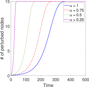
(a)

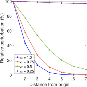
(b)

Figure 3.1: Illustration of the effects of changing the parameter $\alpha$ in the Mittag-Leffler function for the transmission of perturbations in a cycle of 15 nodes.

In closing, the Mittag-Leffler matrix functions, and consequently the use of a fractional-order SI model, are important for modeling the transmission of perturbations across PRNs because they allow to capture important spatial and temporal characteristics of protein perturbations, which are limited with the use of the classical SI model.

4 Computational Results

Here we apply our model to the study of the M^pro of SARS CoV-2 complexed with three inhibitors: PDB codes 6M0K and 6LZE from [8] and 6Y2G from [39]. We compare the results obtained with the free protease structure: PDB 6Y2E. All calculations are carried out on Matlab. For the Mittag-Leffler matrix functions we use the Matlab function “ml_matrix.m” provided by Garrappa and Popolizio [17, 16]. The three inhibitors selected for our study have been reported to display potent inhibitory capacity against SARS CoV-2. This potency is measured through their inhibitory concentration $IC_{50}$, which is the concentration of the inhibitor needed in vitro to inhibit the virus by 50%. For the simulations we use here $\beta=0.01$, $c=0.005,$ $\gamma=1-\frac{c}{n},$ and compare the results for $\alpha=\frac{1}{2}$ and when $\alpha=1$. In Fig. 4.1 we illustrate the time evolution of the number of perturbed amino acids in the complexes studied as well as in the free protease (the last curve is overlapped by that of complex with 6LZE). There are two interesting observations from these plots. First, the use of $\alpha=1/2$ produces a 10-fold reduction of the time needed to reach the steady state of the process, i.e., to perturb 100% of the amino acids in the protease. The second is that the order at which the different complexes reaches 50% of the amino acids perturbed is: 6M0K$<$6LZE$<$6Y2G for both values of $\alpha,$ which is exactly the order of potency of the inhibitors towards SARS CoV-2.

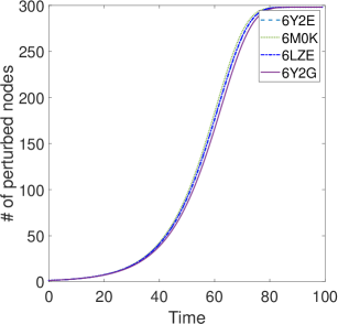
(a)

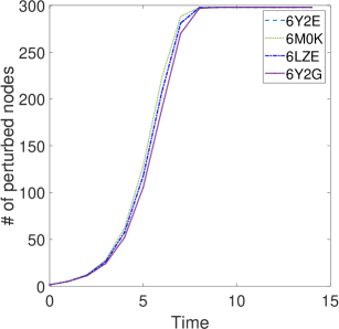
(b)

Figure 4.1: Time evolution of the upper bounds of the normal (a) and fractional (b) SI model for the main protease of CoV-2 bounded to three inhibitors as well as free with $\beta=0.01$, $\gamma=1-\frac{c}{n},$ $c=0.005.$

In order to gain more insights about the influence of the two different dynamics on the propagation of a perturbation across the CoV-2 M^pro when bounded with inhibitors we study the structural contributions from each of the structures to the SI dynamics. In doing so we calculate the relative differences in the individual components of the transmissibility of this perturbation from one residue to another, $G_{ij}^{\alpha}$,

$$\varDelta G_{ij}^{\alpha}=\dfrac{1}{n\left(n-1\right)}\sum_{i\neq j}\dfrac{G_{ij}^{\alpha}\left(\textnormal{bounded}\right)-G_{ij}^{\alpha}\left(\textnormal{free}\right)}{G_{ij}^{\alpha}\left(\textnormal{free}\right)},$$ (4.35)

where $G_{ij}^{\alpha}=[E_{\alpha,1}\biggl{(}(\beta t)^{\alpha}\gamma A\biggr{)}]_{ij}.$

We have selected the time at which 50% of the amino acids in the protease are perturbed, which occurs at $t=6$ ($\alpha=1/2$) and $t=50$ ($\alpha=1$) for doing the calculations. The rest of the parameters remain the same for both descriptors, i.e., $\beta=0.01$, $\gamma=1-\frac{c}{n},$ $c=0.005.$ We also selected the top ten pairs of amino acids according to their values of $\varDelta G_{ij}$. For these pairs we have calculated the average length $\bar{L}$ of the shortest paths connecting the pair of residues. For instance, in 6M0K for $\alpha=1.0$ the largest value of $\varDelta G_{ij}$ is for the pair L167-K269 for which the shortest path has length 8. For the same complex but using $\alpha=0.5$ the largest value of $\varDelta G_{ij}$ is for the pair L167-M276 for which the shortest path has length 10. In addition, we determine which $N_{BS}$ of these pairs of residues in the top ten ranking according to $\varDelta G_{ij}$ is involved directly in the binding site of the protease or it is bounded to one of them. For instance, for the case of the pair before mentioned for 6M0K ($\alpha=1.0$) the residue L167 is directly bounded to two amino acids in the binding site, namely E166 and P168.

	$\alpha=1.0$			$\alpha=0.5$			$IC_{50}$$\left(\mu M\right)$
Inhibitor	$\varDelta G_{ij}$ (%)	$\bar{L}$	$N_{BS}$	$\varDelta G_{ij}$ (%)	$\bar{L}$	$N_{BS}$
6M0K	147.4	8.7	6	70.7	9.1	7	$0.04\pm 0.002$
6LZE	62.3	7.5	6	13.4	8.1	6	$0.053\pm 0.005$
6Y2G	57.2	7.8	6	-4.0	5.8	3	$0.67\pm 0.18$

Table 1: Average change individual transmissibility of perturbations between amino acids in CoV-2 M^pro bounded to inhibitors relative to the free protease. The average path length $\bar{L}$ for paths between the top ten pairs of amino acids according to $\varDelta G_{ij}$ and the number of times a residues in one of these paths is located in the binding site of the protease, $N_{BS}$.

According to the results given in Table 1 we can extract the following conclusions. For $\alpha=1.0$, the values of $\varDelta G_{ij}$ indicate that the three inhibitors increase the transmissibility of perturbations across the protein in relation to the free protease. The trend in these percentages of change is parallel to that of the inhibitory power of the inhibitors. That is, the most potent inhibitor increases more the transmissibility of effects across the protease than the second most powerful one, and the least powerful is the one with the poorer increase in $\varDelta G_{ij}$. However, neither $\bar{L}$ nor $N_{BS}$ display a consistent pattern of change in relation to the values of $IC_{50}$$\left(\mu M\right)$. In contrast, when $\alpha=0.5$ we observe some significant and physically sounded trends for the three parameters studied. First, the most powerful inhibitor increases by 71% the transmissibility of perturbations through the main protease after its binding. It is followed by the second most powerful inhibitor, which increases modestly the transmissibility of perturbations by 13%. However, the weakest inhibitor does not increases, but decreases, the transmissibility of perturbations across the protein. Notice that there is one order of magnitude between the potencies of the first two inhibitors (6M0K and 6LZE) and the third one (6Y2G). In addition, here, the average length of the shortest paths connecting the pairs of residues with the largest increase in the transmissibility of effects follow the same trend as the inhibitory potency. The most potent inhibitor perturbs an average of 9 residues per perturbation path. The second most powerful inhibitor perturbs an average of 8 residues per shortest paths, and the weakest inhibitor perturbs only 6. This is a physically sounded result as the most powerful inhibitor produces a stronger effect on the protease which is “felt” by a larger number of residues in the structure. Finally, it is also remarkable that the number of residues in, or close to, the binding site, correlates with the inhibitory power of the inhibitor. In this case, the most powerful one starts 70% of the most important perturbations according to $\varDelta G_{ij}$ at the binding site, while the weakest initiates only 30% of these perturbations at the binding site.

In terms of the geometric distance between the residues in the perturbed protease we also observe similar characteristics as for the case of the length of the shortest path. For instance, for $\alpha=1$ the average geometric separation of amino acids in the 10 most perturbed pairs is 33.4 Å(6M0K), 28.7 Å(6LZE) and 29.6 Å(6Y2G). Here again we observe a clear lack of correlation with the potency of the inhibitors. However, for $\alpha=0.5$ we have 35.8 Å(6M0K), 30.5 Å(6LZE) and 21.3 Å(6Y2G), in clear agreement with the trend of inhibitory potency of the inhibitors.

5 Conclusions

There are two main conclusions in the current work. The first is that we have proposed a generalized fractional-order SI model which includes the classical SI model as a particular case. We have found an upper bound to the exact solution of this model, which under given initial conditions depends only on the Mittag-Leffler matrix function of the adjacency matrix of the graph. The most important characteristic of this fractional-order SI model is that it allows to account for long-range interactions between the nodes of a network as well as for different time-windows on the transmission of perturbations on networks by tuning the fractional parameter $\alpha$ of the model. Both characteristics are of great relevance in many different applications of complex systems ranging from biological to social systems, and in particular for the study of protein residue networks.

The second main conclusion of this work is that the fractional-order SI model allowed us to extract very important information about the interaction of inhibitors with the main protease of the SARS CoV-2. This structural information consists in the transmission of perturbations produced by the inhibitors at the binding site of the protease to very distant amino acids in other domains of the protein. More importantly, our findings suggest that the length of this transmission seems to reflect the potency of the inhibitor. That is, the more powerful inhibitors transmit perturbations to longer distances through the protein. On the contrary, weaker inhibitors do not propagate such effect beyond 6 edges from the binding site as average. Consequently, these findings are important for understanding the mechanisms of actions of such inhibitors on SARS CoV-2 M^pro and helping in the design of more potent drug candidates against this new coronavirus. Of course, the current approach can be extended and used for the analysis of other inhibitors in other proteins not only using experimental data like in here but using computational analysis of such interactions.

¹Departamento de Matemáticas, Facultad de Ciencias
Universidad de Zaragoza, 50009 Zaragoza, Spain.

e-mail: labadias@unizar.es

²Instituto Universitario de Matemáticas y Aplicaciones
Universidad de Zaragoza, 50009 Zaragoza, Spain.

email: estrada66@unizar.es

³Laboratoire Jacques-Louis Lions, Université Pierre-et-Marie-Curie (UPMC)
4 place Jussieu, 75005, Paris, France.

email: estradarodriguez@ljll.math.upmc.fr

⁴ARAID Foundation, Government of Aragón
50018 Zaragoza, Spain.

email: estrada66@posta.unizar.es

References

- [1] Protein data bank: the single global archive for 3D macromolecular structure data. Nucleic acids research, 47(D1):D520–D528, 2019.
- [2] L. Abadias, E. Alvarez, et al. Uniform stability for fractional Cauchy problems and applications. Topological Methods in Nonlinear Analysis, 52(2):707–728, 2018.
- [3] L. Abadias, C. Lizama, P. J. Miana, et al. Sharp extensions and algebraic properties for solution families of vector-valued differential equations. Banach Journal of Mathematical Analysis, 10(1):169–208, 2016.
- [4] C. N. Angstmann, A. M. Erickson, B. I. Henry, A. V. McGann, J. M. Murray, and J. A. Nichols. Fractional order compartment models. SIAM Journal on Applied Mathematics, 77(2):430–446, 2017.
- [5] E. Bazhlekova. The abstract Cauchy problem for the fractional evolution equation. Fract. Calc. Appl. Anal, 1(3):255–270, 1998.
- [6] H. Berry. Nonequilibrium phase transition in a self-activated biological network. Physical review E, 67(3):031907, 2003.
- [7] A. Cooper and D. Dryden. Allostery without conformational change. European Biophysics Journal, 11(2):103–109, 1984.
- [8] W. Dai, B. Zhang, H. Su, J. Li, Y. Zhao, X. Xie, Z. Jin, F. Liu, C. Li, Y. Li, et al. Structure-based design of antiviral drug candidates targeting the sars-cov-2 main protease. Science, 2020.
- [9] K. Diethelm. The analysis of fractional differential equations: An application-oriented exposition using differential operators of Caputo type. Springer Science & Business Media, 2010.
- [10] K. H. DuBay, J. P. Bothma, and P. L. Geissler. Long-range intra-protein communication can be transmitted by correlated side-chain fluctuations alone. PLoS computational biology, 7(9), 2011.
- [11] E. Estrada. The structure of complex networks: theory and applications. Oxford University Press, 2012.
- [12] E. Estrada. Topological analysis of sars cov-2 main protease. Chaos, in press, 2020.
- [13] E. Estrada and N. Hatano. Communicability in complex networks. Physical Review E, 77(3):036111, 2008.
- [14] E. Estrada and J. A. Rodríguez-Velázquez. Subgraph centrality in complex networks. Phys. Rev. E, 71:056103, May 2005.
- [15] D. Fulger, E. Scalas, and G. Germano. Monte Carlo simulation of uncoupled continuous-time random walks yielding a stochastic solution of the space-time fractional diffusion equation. Physical Review E, 77(2):021122, 2008.
- [16] R. Garrappa. Numerical evaluation of two and three parameter mittag-leffler functions. SIAM Journal on Numerical Analysis, 53(3):1350–1369, 2015.
- [17] R. Garrappa and M. Popolizio. Computing the matrix mittag-leffler function with applications to fractional calculus. Journal of Scientific Computing, 77(1):129–153, 2018.
- [18] R. Gorenflo, A. A. Kilbas, F. Mainardi, S. V. Rogosin, et al. Mittag-Leffler functions, related topics and applications, volume 2. Springer, 2014.
- [19] R. Gorenflo, F. Mainardi, E. Scalas, and M. Raberto. Fractional calculus and continuous-time finance iii: the diffusion limit. In Mathematical finance, pages 171–180. Springer, 2001.
- [20] G. Hu, J. Zhou, W. Yan, J. Chen, and B. Shen. The topology and dynamics of protein complexes: insights from intra–molecular network theory. Current Protein and Peptide Science, 14(2):121–132, 2013.
- [21] V. Latora, V. Nicosia, and G. Russo. Complex networks: principles, methods and applications. Cambridge University Press, 2017.
- [22] A. L. Lee et al. Frameworks for understanding long-range intra-protein communication. Current Protein and Peptide Science, 10(2):116–127, 2009.
- [23] C.-H. Lee, S. Tenneti, and D. Y. Eun. Transient dynamics of epidemic spreading and its mitigation on large networks. In Proceedings of the Twentieth ACM International Symposium on Mobile Ad Hoc Networking and Computing, pages 191–200, 2019.
- [24] S. Lu, M. Ji, D. Ni, and J. Zhang. Discovery of hidden allosteric sites as novel targets for allosteric drug design. Drug discovery today, 23(2):359–365, 2018.
- [25] F. Mainardi. Fractional calculus and waves in linear viscoelasticity: an introduction to mathematical models. World Scientific, 2010.
- [26] F. Mainardi and R. Gorenflo. On mittag-leffler-type functions in fractional evolution processes. Journal of Computational and Applied Mathematics, 118(1-2):283–299, 2000.
- [27] I. Matychyn. On computation of matrix Mittag-Leffler function. arXiv preprint arXiv:1706.01538, 2017.
- [28] W. Mei, S. Mohagheghi, S. Zampieri, and F. Bullo. On the dynamics of deterministic epidemic propagation over networks. Annual Reviews in Control, 44:116–128, 2017.
- [29] M. Miotto, L. Di Rienzo, P. Corsi, D. Raimondo, and E. Milanetti. Simulated epidemics in 3d protein structures to detect functional properties. arXiv preprint arXiv:1906.05390, 2019.
- [30] S. K. Mishra, M. Gupta, and D. K. Upadhyay. Fractional derivative of logarithmic function and its applications as multipurpose asp circuit. Analog Integrated Circuits and Signal Processing, 100(2):377–387, 2019.
- [31] D. Mugnolo. Dynamical systems associated with adjacency matrices. arXiv preprint arXiv:1702.05253, 2017.
- [32] K. M. Ottemann, W. Xiao, Y.-K. Shin, and D. E. Koshland. A piston model for transmembrane signaling of the aspartate receptor. Science, 285(5434):1751–1754, 1999.
- [33] R. Paris. Exponential asymptotics of the mittag–leffler function. Proceedings of the Royal Society of London. Series A: Mathematical, Physical and Engineering Sciences, 458(2028):3041–3052, 2002.
- [34] I. Podlubny. Fractional differential equations: an introduction to fractional derivatives, fractional differential equations, to methods of their solution and some of their applications. Elsevier, 1998.
- [35] A. Sadeghi and J. R. Cardoso. Some notes on properties of the matrix Mittag-Leffler function. Applied Mathematics and Computation, 338:733–738, 2018.
- [36] C. S. G. The International et al. The species severe acute respiratory syndrome-related coronavirus: classifying 2019-ncov and naming it SARS-CoV-2. Nature Microbiology, page 1, 2020.
- [37] F. Wu, S. Zhao, B. Yu, Y.-M. Chen, et al. A new coronavirus associated with human respiratory disease in China. Nature, 579(7798):265–269, 2020.
- [38] Y. Xu and M. Havenith. Perspective: Watching low-frequency vibrations of water in biomolecular recognition by thz spectroscopy. The Journal of chemical physics, 143(17):170901, 2015.
- [39] L. Zhang, D. Lin, X. Sun, U. Curth, C. Drosten, L. Sauerhering, S. Becker, K. Rox, and R. Hilgenfeld. Crystal structure of SARS-CoV-2 main protease provides a basis for design of improved -ketoamide inhibitors. Science, 2020.
- [40] P. Zhou, X.-L. Yang, X.-G. Wang, B. Hu, et al. A pneumonia outbreak associated with a new coronavirus of probable bat origin. Nature, 579(7798):270–273, 2020.