A branch-and-Benders-cut algorithm for a bi-objective stochastic facility location problem

Abstract

In many real-world optimization problems, more than one objective plays a role and input parameters are subject to uncertainty. In this paper, motivated by applications in disaster relief and public facility location, we model and solve a bi-objective stochastic facility location problem. The considered objectives are cost and uncovered demand, whereas the demand at the different population centers is uncertain but its probability distribution is known. The latter information is used to produce a set of scenarios. In order to solve the underlying optimization problem, we apply a Benders’ type decomposition approach which is known as the L-shaped method for stochastic programming and we embed it into a recently developed branch-and-bound framework for bi-objective integer optimization. We analyze and compare different cut generation schemes and we show how they affect lower bound set computations, so as to identify the best performing approach. Finally, we compare the branch-and-Benders-cut approach to a straight-forward branch-and-bound implementation based on the deterministic equivalent formulation.

1 Introduction

Facility location problems play an important role in long-term public infrastructure planning. Prominent examples concern the location of fire departments, schools, post offices, or hospitals. They are not only relevant in public (or former public) infrastructure planning decisions in “regular” planning situations: they are also of concern in the context of emergency planning, e.g., relief goods distribution in the aftermath of a disaster or preparation for slow onset disasters such as droughts. In many of these contexts, accurate demand figures are not available; assumed demand values rely on estimates, while their actual realizations depend, e.g., on the severity of the slow onset disaster, the demographic population development in an urban district, etc. Since facility location decisions are usually long-term investments, the uncertainty involved in the demand figures should already be taken into account at the planning stage.

Another important issue is that facility location problems often involve several objectives. On the one hand, client-oriented objectives should be optimized. For example, in cases where it is not possible to satisfy the demand to 100 percent, the total covered demand should be as high as possible. On the other hand, cost considerations also play a role. This implies that decision makers face a trade-off between client-oriented and cost-oriented goals. Instead of combining these two usually conflicting measures into one objective function, it is advisable to elucidate their trade-off relationship. Such an approach provides valuable information to the involved stakeholders and allows for better informed decisions. Following this line of thought, in this paper, we model a bi-objective stochastic facility location problem that considers cost and coverage as two competing but concurrently analyzed objectives. Furthermore, we incorporate stochastic information on possible realizations of the considered demand figures in the form of scenarios sampled from probability distributions.

Motivated by recent advances in exact methods for multi-objective integer programming, we solve this problem by combining a recently developed bi-objective branch-and-bound algorithm (Parragh and Tricoire,, 2019) with the L-shaped method (Van Slyke and Wets,, 1969), which applies Benders decomposition (Benders,, 1962) to two-stage stochastic programming problems. We integrate several enhancements, such as partial decomposition, and we compare the resulting approach to using a deterministic equivalent formulation within the same branch-and-bound framework.

This paper is organized as follows. In Section 2, we give a short overview of related work in the field of bi-objective (stochastic) facility location. In Section 3, we define the bi-objective stochastic facility location problem (BOSFLP) that is subject to investigation in this paper and we discuss L-shaped based decomposition approaches of the proposed model. In Section 4 we explain how we integrate the proposed decomposition schemes into the bi-objective branch-and-bound framework. A computational study comparing the different approaches is reported in Section 5, and Section 6 concludes the paper and provides directions for future research.

2 Related work

Our problem is a stochastic extension of a bi-objective maximal covering location problem (MCLP). The MCLP has been introduced in Church and ReVelle, (1974). It consists in finding locations for a set of $p$ facilities in such a way that a maximum population can be served within a pre-defined service distance. Obviously, in this classical formulation, the number of facilities that are to be opened is a cost measure, and the total population that can be served is a measure of demand coverage. Thus, cost occurs in a constraint, whereas the objective represents covered demand. It is natural to extend this problem to a bi-objective covering location problem (CLP) where both cost (to be minimized) and covered demand (to be maximized) are objectives. Indeed, bi-objective CLPs of this kind have been studied in several papers, see e.g. Bhaskaran and Turnquist, (1990), Harewood et al., (2002), Villegas et al., (2006), or Gutjahr and Dzubur, (2016); for further articles, we refer to Farahani et al., (2010).

Another strand of literature relevant in the present context addresses bi-objective covering tour problems (CTPs). One of the oldest CTP models, that of the maximal covering tour problem (MCTP) introduced by Current and Schilling, (1994), has already been cast in the form of a bi-objective problem. A fixed number of nodes have to be selected out of the nodes of a given transportation network for being visited by a vehicle, and a tour on these visited nodes has to be determined. The objectives are minimization of the total tour length (a cost measure) and maximization of the total demand that is satisfied within some pre-specified distance from a visited node (a measure of demand coverage).

Other multi-objective CTP formulations can be found in the following papers: Jozefowiez et al., (2007) deal with a bi-objective CTP where the second objective function of the MCTP is replaced by the largest distance between a node of some given set and the nearest visited node. Doerner et al., (2007) develop a three-objective CTP model for mobile health care units in a developing country. Nolz et al., (2010) study a multi-objective CTP addressing the problem of delivery of drinking water to the affected population in a post-disaster situation.

Most importantly for the present work, Tricoire et al., (2012) generalize the bi-objective CTP to the stochastic case by assuming uncertainty on demand. The aim is to support the choice of distribution centers (DCs) for relief commodities and of delivery tours supplying the DCs from a central depot. Demand in population nodes is assumed as uncertain and modeled stochastically. DCs have fixed given capacities, as well as vehicles. The model considers two objective functions: The first objective is cost (more precisely, the sum of opening costs for DCs and of transportation costs), and the second is expected uncovered demand. Contrary to basic covering tour models supposing a fixed distance threshold, uncovered demand is defined by the more general model assumption that the percentage of individuals who are able and willing to go to the nearest DC can be represented by a nonincreasing function of the distance to this DC. Both the demand of those individuals who stay at home and the demand of those individuals who are not supplied in a DC because of DC capacity and/or vehicle capacity limits contribute to the total uncovered demand. Because of the uncertainty on the actual demand, total uncovered demand is a random variable, the expected value of which defines the second objective function to be minimized.

The problem investigated in the present paper generalizes the bi-objective CLP to a stochastic bi-objective problem by considering demand as uncertain and modelling it by a probability distribution, in an analogous way as in Tricoire et al., (2012). Alternatively, the investigated problem can also be derived from a CTP by omitting the routing decisions and generalizing the resulting bi-objective location problem again to the stochastic case. From the viewpoint of the latter consideration, the current model can be seen as related to the special case of the problem of Tricoire et al., (2012) obtained by neglecting routing costs. However, the current model builds on refined assumptions concerning the decision structure of the two-stage stochastic program which makes the second-stage optimization problem nontrivial, contrary to Tricoire et al., (2012) where the second-stage optimization problem can be solved by elementary calculations.

Multi-objective stochastic optimization (MOSO) problems, though of eminent importance for diverse practical applications, are investigated in a more limited number of publications, compared to the vast amount of literature both on multi-objective optimization and on stochastic optimization; for surveys on MOSO, we refer the reader to Caballero et al., (2004), Abdelaziz, (2012), and Gutjahr and Pichler, (2016). Of special relevance for our present work are multi-objective two-stage stochastic programming models where the “multicriteria” solution concept is that of the determination of Pareto-efficient solutions, and where the first-stage decision contains integer decision variables. Most papers in this area assume that one of the two objectives only depends on the first-stage decision, whereas the other objective depends on the decisions in both stages. This holds also for Tricoire et al., (2012). Let us give two other examples: Fonseca et al., (2010) present a two-stage stochastic bi-objective mixed integer program for reverse logistics, with strategic decisions on location and function of diverse collection and recovery centers in the first stage, and tactical decisions on the flow of disposal from clients to centers or between centers in the second stage. The first objective is expected total cost, which depends both on the first-stage and second-stage decision, whereas the second objective, the obnoxious effect on the environment, only depends on the first-stage decision. Stochasticity is associated with waste generation and with transportation costs. Cardona-Valdés et al., (2011) deal with decisions on the location of DCs and on transportation flows in a two-echelon production distribution network. Uncertainty holds with respect to the demand. The first objective represents expected costs, whereas the second objective expresses the sum of the maximum lead times from plants to customers. The authors model the random distribution by scenarios and solve the two-stage programming model by the L-shaped method, a technique that we will also use in our present work.

Our problem has a structure similar to the models cited above: while the covered demand depends on the decisions in both stages, the cost objective is already determined by the first-stage decision. This allows the development of an efficient solution algorithm. Contrary to Tricoire et al., (2012), we will not apply an epsilon-constraint method for the determination of Pareto-efficient solutions, but use instead a more recent method developed in Parragh and Tricoire, (2019).

Finally, let us mention that the humanitarian logistics literature, which tackles facility location problems under high uncertainty and multiple objectives, has been relatively prolific with regards to multi-objective stochastic optimization models and corresponding solution techniques (cf. Gutjahr and Nolz, (2016)). Let us give two examples of papers using both Pareto optimization and two-stage stochastic programs. Khorsi et al., (2013) propose a bi-objective model with objectives “weighted unsatisfied demand” and “expected cost”. Discrete scenarios from a set of possible disaster situations are applied to represent uncertainty. The epsilon-constraint method is used to solve the model. Rath et al., (2016) deal with the uncertain accessibility of transportation links and develop a two-stage stochastic programming model where in the first stage decisions on the locations of distribution centers have to be made, and in the second stage (based on current information on road availability) the transportation flows have to be organized. Objective functions are expected total cost and expected covered demand. The structure of the two-stage stochastic program is different from that in the current paper insofar as both objectives depend on both first-stage and second-stage decision variables, which requires specific (and computationally less efficient) solution techniques. For general information on humanitarian logistics, the reader is referred to the standard textbook by Tomasini and Van Wassenhove, (2009). Two-stage stochastic programing approaches to this field (in a single-objective context) are reviewed in Grass and Fischer, (2016). A good recent example for the application of Benders decomposition to a stochastic model for humanitarian relief network design is Elçi and Noyan, (2018).

For an overview on facility location in general, we refer the reader to Hamacher and Drezner, (2002). Standard textbooks on multi-objective optimization and on stochastic programming are Ehrgott, (2005) and Birge and Louveaux, (2011), respectively.

3 Problem definition and decomposition

In the bi-objective stochastic facility location problem (BOSFLP) considered in this article, the demand at each node $i\in V$ is uncertain. We denote by $W_{i}$ the demand at node $i$, by ${\mathbf{E}}(W_{i})=w_{i}$ the expected demand at node $i$ and by $\xi_{i}$ a random variable such that $W_{i}=\xi_{i}w_{i}$. At each node $j$, a facility may be built. A facility at node $j$ has a capacity $\gamma_{j}$ and operating costs $c_{j}$. Furthermore, facilities that are farther than a certain maximum distance $d_{max}$ from a demand point may not be used to cover it. In order to take this aspect into account, we consider the set $A=\{(i,j)|i,j\in V,d_{ij}\leq d_{max}\}$ of possible assignments $(i,j)$, where $d_{ij}$ denotes the distance of demand node $i$ from a potential facility at node $j$. The two considered goals are to minimize the total costs for operating facilities and to maximize the expected covered demand. Using the following decision variables,

$$z_{j}= \begin{cases}1$ if a facility is built at node $j$ and $\cr 0$, otherwise.$\end{cases}$$

$$y_{ij} \text{ demand of population node $i$ covered by facility $j$},$$

$$u_{j} j$$ total demand covered by facility .

we formulate the BOSFLP as a two-stage stochastic program:

$$\min f_{1} =\sum_{j\in V}c_{j}z_{j}$$ (1)

$$\min f_{2} ={\mathbf{E}}(Q(z,\xi))$$ (2)

$$z_{j} \in\{0,1\} \forall j\in V.$$ (3)

Second stage:

$$Q(z,\xi) =\min_{u}(-\sum_{j\in V}u_{j})$$ (4)

subject to:

$$u_{j} \leq\sum_{i|(i,j)\in A}y_{ij} \forall j\in V,$$ (5)

$$u_{j} \leq\gamma_{j}z_{j} \forall j\in V,$$ (6)

$$y_{ij} \leq W_{i}z_{j} \forall(i,j)\in A,$$ (7)

$$\sum_{j|(i,j)\in A}y_{ij} \leq W_{i} \forall i\in V,$$ (8)

$$0 \leq y_{ij} \forall(i,j)\in A,$$ (9)

$$0 \leq u_{j} \forall j\in V.$$ (10)

Objective function (1) minimizes the total facility opening costs. Objective function (2) maximizes the expected covered demand. In order to obtain two minimization objectives, objective (2) has been multiplied by $(-1)$. Note that maximization of the expected covered demand is equivalent to minimization of the expected uncovered demand, since the expected demand is a constant. The first stage model only comprises one set of constraints which require that all $z_{j}$ variables may only take values $0$ or $1$. The second stage model consists of the objective function given in (4), representing the negative value of the total covered demand, and a number of constraints which determine the maximum possible coverage given a first stage solution. Constraints (5) link the coverage variables with the assignment variables: the covered demand at node $j$ cannot be larger than the actual demand assigned to this node. Constraints (6) make sure that the capacity of facility $j$ is not exceeded. Constraints (7) guarantee that a demand node can only be assigned to a facility if the respective facility is open. Finally, constraints (8) ensure that any part of the demand at $i$ is only covered at most once. The variables $z_{j}$ are first-stage decision variables whereas the variables $y_{ij}$ are second-stage decision variables, i.e. the latter variables can depend on the realizations of the demand values; that is, $y_{i}=y_{i}(\xi)$. Similarly, $u_{j}=u_{j}(\xi)$ and $W_{i}=W_{i}(\xi)$.

In this paper, we use a discrete set of scenarios (with equal probabilities) in order to approximate the (joint) probability distribution of the demand as estimated by the decision maker. If a Monte-Carlo simulation procedure is available for simulating demand, each realization of this procedure can be taken as a scenario. Let $N$ denote this set of scenarios. Then, using an additional index $\nu$ to denote a given scenario for the variables of the second stage problem, we obtain the following expanded or deterministic equivalent model:

$$\min f_{1} =\sum_{j\in V}c_{j}z_{j}$$ (11)

$$\min f_{2} =-\frac{1}{|N|}\sum_{\nu\in N}\sum_{j\in V}u_{j}^{\nu}$$ (12)

subject to:

$$u_{j}^{\nu} \leq\sum_{i|(i,j)\in A}y_{ij}^{\nu} \forall j\in V,\nu\in N,$$ (13)

$$u_{j}^{\nu} \leq\gamma_{j}z_{j} \forall j\in V,\nu\in N,$$ (14)

$$y_{ij}^{\nu} \leq W_{i}^{\nu}z_{j} \forall(i,j)\in A,\nu\in N,$$ (15)

$$\sum_{j|(i,j)\in A}y_{ij}^{\nu} \leq W_{i}^{\nu} \forall i\in V,{\nu}\in N,$$ (16)

$$0 \leq y_{ij}^{\nu} \forall(i,j)\in A,\nu\in N,$$ (17)

$$0 \leq u_{j}^{\nu} \forall j\in V,\nu\in N,$$ (18)

$$z_{j} \in\{0,1\} \forall j\in V.$$ (19)

This problem formulation decomposes by scenario and the L-shaped method, as introduced by Van Slyke and Wets, (1969), can be used to solve its linear relaxation. The L-shaped method relies on a master problem and one subproblem per scenario whereas the information from the subproblem is incorporated into the master problem by means of cutting planes. We distinguish feasibility and optimality cuts. In the case of complete recourse, as is the case for our problem, only optimality cuts have to be added: the solution to the first stage problem will always allow a feasible solution to the second stage problem. (This holds for our problem, since setting $y_{ij}$ and $u_{j}$ to zero produces a feasible solution.)

More precisely, using variable $\theta$ to represent the second stage objective, we obtain the following master linear program (LP):

$$\min f_{1}= \sum_{j\in V}c_{j}z_{j}$$ (20)

$$\min f_{2}= \>\theta$$ (21)

subject to:

$$-\sum_{i\in V}\max_{\nu\in N}\{W^{\nu}_{i}\} \leq\theta$$ (22)

$$0\leq z_{j} \leq 1 \forall j\in V$$ (23)

where $-\sum\limits_{i\in V}\max\limits_{\nu\in N}\{W^{\nu}_{i}\}$ provides a valid bound on $\theta$, since $Q(z,\xi)=\min\limits_{u}(-\sum\limits_{j\in V}u_{j})\geq-\sum\limits_{i\in V}\max\limits_{\nu\in N}\{W^{\nu}_{i}\}$.

As explained in Section 4, the two objectives are combined into a weighted sum and the resulting single-objective LP is iteratively solved with different weights in order to enumerate the set of efficient solutions. In that context and for a given set of weights, to determine if the obtained solution to the master weighted-sum LP is optimal, we check if optimality cuts have to be added. We denote by $z_{j}^{l}$ and $\theta^{l}$ the variable values obtained from solving the master LP and we solve for each $\nu\in N$ the following model:

$$\min(-\sum_{j\in V}u_{j})$$ (24)

subject to:

$$u_{j} \leq\sum_{i|(i,j)\in A}y_{ij} \forall j\in V,$$ (25)

$$u_{j} \leq\gamma_{j}z^{l}_{j} \forall j\in V,$$ (26)

$$y_{ij} \leq W_{i}^{\nu}z^{l}_{j} \forall(i,j)\in A,$$ (27)

$$\sum_{j|(i,j)\in A}y_{ij} \leq W_{i}^{\nu} \forall i\in V,$$ (28)

$$0 \leq y_{ij} \forall(i,j)\in A,$$ (29)

$$0 \leq u_{j} \forall j\in V.$$ (30)

Let $\mathcal{Q}(z)={\mathbf{E}}_{\xi}Q(z,\xi)$. If $\mathcal{Q}(z^{l})\leq\theta^{l}$, we terminate: optimality has been reached. Otherwise, we generate an optimality cut. Optimality cuts rely on dual information. To write the dual of the above model (24) – (30), we denote by $\lambda_{j}$ the dual variables of constraints (25), by $\pi^{l}_{j}$ the dual variables of constraints (26), by $\sigma_{ij}$ the dual variables of constraints (27), and by $\delta_{i}$ the dual variables of constraints (28):

$$\max(-\sum_{j\in V}\pi_{j}\gamma_{j}z_{j}^{l}-\sum_{(i,j)\in A}\sigma_{ij}W_{i}^{\nu}z_{j}^{l}-\sum_{i\in V}W_{i}^{\nu}\delta_{i})$$ (31)

subject to:

$$\lambda_{j}+\pi_{j} \geq 1 \forall j\in V,$$ (32)

$$\lambda_{j}-\sigma_{ij}-\delta_{i} \leq 0 \forall(i,j)\in A,$$ (33)

$$\lambda_{j} \geq 0 \forall j\in V,$$ (34)

$$\pi_{j} \geq 0 \forall j\in V,$$ (35)

$$\sigma_{ij} \geq 0 \forall(i,j)\in A,$$ (36)

$$\delta_{i} \geq 0 \forall i\in V,$$ (37)

With a bit of abuse of notation, we denote by $\pi_{j}(\xi^{\nu})$, $\sigma_{ij}(\xi^{\nu})$, and $\delta_{i}(\xi^{\nu})$ the dual variable values for a given scenario $\nu$ and the objective function value by $Q(z^{l},\xi^{\nu})=-\sum_{j\in V}\pi_{j}(\xi^{\nu})\gamma_{j}z_{j}^{l}-\sum_{(i,j)\in A}\sigma_{ij}(\xi^{\nu})W_{i}^{\nu}z_{j}^{l}-\sum_{i\in V}W_{i}^{\nu}\delta_{i}(\xi^{\nu})$. Then, the optimality cut is of the following form:

$$Q(z,\xi^{\nu})\geq Q(z^{l},\xi^{\nu}) +\big{(}\big{[}-\sum_{j\in V}\pi_{j}(\xi^{\nu})\gamma_{j}z_{j}-\sum_{(i,j)\in A}\sigma_{ij}(\xi^{\nu})W_{i}^{\nu}z_{j}-\sum_{i\in V}\delta_{i}(\xi^{\nu})W_{i}^{\nu}\big{]}$$ (38)

$$-\big{[}-\sum_{j\in V}\pi_{j}(\xi^{\nu})\gamma_{j}z_{j}^{l}-\sum_{(i,j)\in A}\sigma_{ij}(\xi^{\nu})W_{i}^{\nu}z_{j}^{l}-\sum_{i\in V}\delta_{i}(\xi^{\nu})W_{i}^{\nu}\big{]}\big{)}$$

Rearranging the terms, we obtain

$$Q(z,\xi^{\nu})\geq Q(z^{l},\xi^{\nu})+\big{(}\sum_{j\in V}\pi_{j}(\xi^{\nu})\gamma_{j}(z_{j}^{l}-z_{j})+\sum_{(i,j)\in A}\sigma_{ij}(\xi^{\nu})W_{i}^{\nu}(z_{j}^{l}-z_{j})\big{)}$$ (39)

Finally, combining over all scenarios, we obtain the optimality cut for the expected second stage objective function (with $\bar{\pi}_{j}=1/|N|\sum_{\nu}\pi_{j}(\xi^{\nu})$ and $\bar{\sigma}_{ij}=1/|N|\sum_{\nu}\sigma_{ij}(\xi^{\nu})W_{i}^{\nu}$):

$$\theta\geq\mathcal{Q}(z^{l})+\big{(}\sum_{j\in V}\bar{\pi}_{j}\gamma_{j}(z_{j}^{l}-z_{j})+\sum_{(i,j)\in A}\bar{\sigma}_{ij}(z_{j}^{l}-z_{j})\big{)}$$ (40)

Alternatively, instead of adding one optimality cut per iteration, we can also add one cut per scenario. In order to do so, a separate variable $\theta^{\nu}$ for each scenario $\nu$ has to be used, resulting in the following master LP:

$$\min f_{1}= \sum_{j\in V}c_{j}z_{j}$$ (41)

$$\min f_{2}= \frac{1}{N}\sum_{\nu\in N}\theta^{\nu}$$ (42)

subject to:

$$-\sum_{i\in V}W_{i}^{\nu} \leq\theta^{\nu}\leq 0 \forall\nu\in N$$ (43)

$$0 \leq z_{j}\leq 1 \forall j\in V$$ (44)

Then, we check each subproblem and add a cut of the form (39) in the case where $\theta^{\nu,l}<Q(z^{l},\xi^{\nu})$. In the case where all scenarios are checked and no additional cut has to be added, optimality has been reached.

4 Solution methods

In order to solve the BOSFLP, we integrate L-shaped based cut generation into the recently introduced bi-objective branch-and-bound framework of Parragh and Tricoire, (2019). In what follows, we first describe the key ingredients of the branch-and-bound framework and thereafter how we combine it with the L-shaped method.

4.1 Bi-objective branch-and-bound

Without loss of generality, we consider a bi-objective minimization problem. The bi-objective branch-and-bound (BIOBAB) algorithm of Parragh and Tricoire, (2019) generalizes the single-objective concept of branch-and-bound to two objectives. We first introduce the notion of lower and upper bound set. Thereafter, we explain the main loop of the algorithm and we describe several enhancements.

4.1.1 Lower and upper bound sets

During the execution of the BIOBAB algorithm, instead of single numerical values, upper and lower bound sets are computed. These rely on the notion of bound set introduced by Ehrgott and Gandibleux, (2006). A subset $L$ of the objective space is called a lower bound set of the feasible set $Y$ in objective space if $\forall y\in Y\exists x\in L:y\geq x$, where $y\geq x$ iff $y_{i}\geq x_{i}(i=1,2)$. Starting from the root node, at each node of the branch-and-bound tree, a lower bound (LB) set is calculated. The special LB set we use corresponds to the lower left boundary of the convex hull of the feasible set of the current node LP in objective space. This boundary can be described by its corner points which can be efficiently computed by means of an algorithm that is similar to that of Aneja and Nair, (1979). This algorithm consists in solving a series of single-objective weighted-sum problems by systematically enumerating a finite set of weight combinations. In our case, this means that the two objectives are combined into a weighted sum and we solve a (linear) relaxation of the weighted-sum problem with the appropriate weight combination at every step of the LB generation algorithm. The image of the solution to each relaxed weighted-sum problem gives a corner point of the boundary in objective space. In a first step, the algorithm computes the two extreme solutions, i.e., the best solution optimizing $f_{1}$ and the best solution optimizing $f_{2}$. Let $a$ denote the point in objective space which is the image of the optimal solution for $f_{1}$ and $b$ the point in objective space which is the image of the optimal solution for $f_{2}$. In order to obtain the best possible value for the respective other objective function, lexicographic minimization is used. The next step consists in identifying the weights for finding the next solution of the LB set. These weights are derived from $a$ and $b$. Let $a_{1}$ and $a_{2}$ denote the coordinates of $a$ and $b_{1}$ and $b_{2}$ the coordinates of $b$. Then the weights to obtain the next solution of the LB set are $w_{2}=b_{1}-a_{1}$ and $w_{1}=a_{2}-b_{2}$. Let the image of this new solution in objective space be denoted by $c$. Then we look for additional solutions between $a$ and $c$ and between $c$ and $b$, in the same way as before. For further details we refer to Parragh and Tricoire, (2019).

The thus obtained LB set is then filtered using a set of known solutions, called the upper bound (UB) set. The UB set corresponds to all integer feasible solutions obtained during the search that have not been found to be dominated so far. In order to fathom a node, the whole LB set of this node must be dominated by the UB set. Note that the LB set and the UB set are conceptually different; while the former is a continuous set, the latter is a discrete set. This is illustrated in Figure 1. In the example of Figure 1, the current node cannot be fathomed since the UB set does not dominate the LB set.

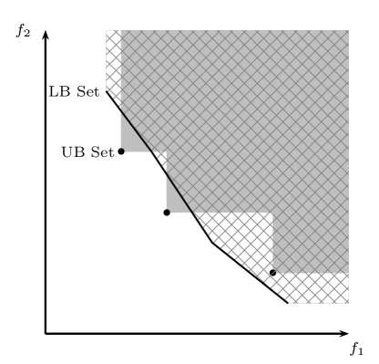
Figure 1: LB set (continuous) of a given branch-and-bound node, current UB set (dots), region dominated by LB set (grid pattern), region dominated by UB set (gray) in objective space. Non-dominated feasible solutions have to lie in the white grid-pattern area.

4.1.2 Tree generation and branching rules

Algorithm 1 shows the main loop of the BIOBAB algorithm. Function $push(C,x)$ adds $x$ to an existing collection of nodes $C$ and function $pop(C)$ retrieves a node from $C$. They are used to add and retrieve the nodes of the branch-and-bound tree. A node in the branch-and-bound tree represents a set of branching decisions. Depending on the data structure employed for $C$, different tree exploration strategies can be obtained. We use depth-first search. The algorithm can take a starting UB set as input in order to speed up the search. In our case, the UB set passed to the algorithm is empty and it is updated every time a new integer solution is found.

Algorithm 1 $BIOBAB(UB)$

1:  $rootNode\leftarrow\emptyset$

2:  $C\leftarrow\emptyset$

3:  $push(C,rootNode)$

4:  while $C\neq\emptyset$ do

5:     $node\leftarrow pop(C)$

6:     $LB\leftarrow bound(node,UB)$

7:     $LB\leftarrow filter(LB,UB)$

8:     if $LB\neq\emptyset$ then

9:        $newBranches\leftarrow branch(LB)$

10:        for all $decision\in newBranches$ do

11:           $push(C,node\cup\{decision\})$

12:        end for

13:     end if

14:  end while

15:  return  $UB$

A key component of the BIOBAB algorithm of Parragh and Tricoire, (2019) is a branching rule that works on the objective space, which is referred to as objective space branching. It allows to discard dominated regions of the search space even if a given node cannot be fathomed. The information whether or not objective space branching can be performed is obtained in the filtering step: whenever the current UB set allows to discard regions from the lower bound set and the resulting LB set is discontinuous, objective space branching in combination with variable branching is performed and each new branch (or node) corresponds to a different continuous subset of the discontinuous LB set. In the example depicted in Figure 1, the filtering operation results in a discontinuous LB set consisting of three continuous subsets.

Whenever the filtered LB set is not discontinuous, standard variable branching rules are applied. In this case, the binary variable to branch on is selected based on information from all corner point solutions of the LB set: the variable that is fractional in the highest amount of corner points is selected for branching. Ties are broken by selecting the variable with lowest average distance to 0.5. If this is not enough, ties are broken by selecting the variable whose average value has the lowest distance to 0.5.

4.1.3 Enhanced objective space filtering

Another key component of the algorithm of Parragh and Tricoire, (2019) are enhanced objective space filtering rules that rely on the observation that the objective values of integer solutions may only take certain values. In the simplest case, they are restricted to integer values. In Parragh and Tricoire, (2019), only integer problems are addressed, where all coefficients in the objective function may only assume integer values. In this case, it is easy to observe that integer solutions may only assume integer objective values. In this paper, we solve a mixed integer program (the $y_{ij}$ and $u_{j}$ variables may assume fractional values). However, the continuous variables only appear in the second objective function. Thus, for the first objective function the same reasoning as in Parragh and Tricoire, (2019) can be used. Our second objective function depends on continuous variables and, in addition, we divide by the number of scenarios to obtain the expected value. However, we can still exploit the ideas of Parragh and Tricoire, (2019). The reasoning is as follows. Let us assume that all coefficients are integer valued (both in the constraints and in the objective functions). This implies that the capacities $\gamma_{j}$ of the distribution centers are integer valued as well as the demands at the demand nodes $W_{i}$. Then, it is easy to see that, in any optimal solution for a given scenario, at each distribution center, either the capacities are fully used (we maximize covered demand) or, in the case of excessive capacities, the entire demand of the reachable demand nodes is covered, resulting in an integer valued objective function. Now, fractional values can only be due to the term $1/|N|$. Since this term is constant, we can simply multiply the second objective function by $|N|$ to obtain integer valued results. If we do not want to do that, the constant term $1/|N|$ still allows us to know the granularity of the admissible values of the objective function; any region in the objective space which does not contain any admissible values can be removed from further consideration. This observation can be used to prune LB segments and to speed up the LB set computation procedure. For further details we refer to Parragh and Tricoire, (2019).

4.2 Lower bound set generation and integration with L-shaped method

Integrating the L-shaped method into BIOBAB mainly affects the lower bound set generation scheme. In what follows we first present the employed master program and then the employed cut generation strategies.

4.2.1 Master program

In a first step, we set up the master LP. Let $w_{1}$ and $w_{2}$ denote the weights as described in 4.1.1 and $\bar{f}_{1}$ and $\bar{f}_{2}$ the upper bounds on $f_{1}$ and $f_{2}$ respectively, we obtain the following generic master LP for the multi-cut version:

$$\min w_{1}\sum_{j\in V}c_{j}z_{j}+w_{2}\frac{1}{|N|}\sum_{\nu\in N}\theta^{\nu}$$ (45)

subject to:

$$-\sum_{i\in V}W_{i}^{\nu}\leq\theta^{\nu} \leq 0 \forall\nu\in N$$ (46)

$$\sum_{j\in V}c_{j}z_{j} \leq\bar{f}_{1}$$ (47)

$$\frac{1}{|N|}\sum_{\nu\in N}\theta^{\nu} \leq\bar{f}_{2}$$ (48)

$$0\leq z_{j} \leq 1 \forall j\in V$$ (49)

To obtain the single cut version of the master LP, $1/|N|\sum\limits_{\nu\in N}\theta^{\nu}$ has to be replaced by $\theta$. However, preliminary experiments indicated that, as expected, the multi-cut version performs better than the single cut version. For that reason, we focus on the multi-cut version. The model features bounds on both objectives to allow for easy updates in the case of objective space branching, which is realized by updating these bounds to discard dominated regions of the objective space. The weights in the objective function are determined by the algorithm of Aneja and Nair, (1979). For each weight combination the L-shaped method is applied, i.e. optimality cuts (see Section 3) are generated as explained in the subsequent Section.

In order to strenghten the above master LP, we can use the following valid inequalities:

$$-\sum_{j\in V}z_{j}\gamma_{j} \leq\theta^{\nu} \forall\nu\in N$$ (50)

They rely on the fact that the maximum coverage level is bounded by the total capacity of the number of opened facilities. By doing so, in the case where capacities are tight, we anticipate that fewer optimality cuts have to be added.

4.2.2 Optimality cut generation strategies

In the general case, the master program is solved, each scenario subproblem is solved and in the case where $\theta^{\nu}$ is currently under-estimated an optimality cut is added and the master program is solved again. Optimality is attained if no additional cut has to be added. However, it is clearly not necessary to check all scenarios for valid cuts at each iteration: we can stop cut generation as soon as at least one cut has been found. In order to do so, several strategies can be envisaged and our preliminary experiments showed that the following strategy works reasonably well: at each call to the optimality cut generation routine, we do not start to check for cuts with the first scenario but we start with the scenario following the last scenario for which a cut was generated, i.e. if scenario 2 generated the last cut, in the next iteration we check scenario 3 first and iterate over the scenarios such that scenario 2 is the one checked last. This way, we always check first one of the scenarios that have not been checked for the longest time. In terms of cut management, we maintain a global cut pool and we keep all generated cuts in this pool.

In the single objective case it has been observed, e.g. by Adulyasak et al., (2015), that considerable performance gains are achieved if optimality cuts are only generated at incumbent solutions. Motivated by the success in the single objective domain, we transfer this idea to multi-objective optimization. We recall that we generate bound sets which are obtained by systematically solving a series of weighted-sum problems. In the current context, each weighted-sum problem corresponds to solving the above master program with the L-shaped method. In the case where fewer optimality cuts than necessary or even no optimality cuts are added, objective two is under-estimated and therefore we have a valid lower bound on the true value of objective two. This means that we do not really need to generate optimality cuts at each weighted-sum solution but we can restrict cut generation to those weighted-sum solutions which are integer feasible (mimicking the idea of adding cuts only at incumbent solutions). In the following we denote such a solution as an incumbent solution.

In the case where we find an incumbent solution, we do generate cuts then re-solve the modified LP with the same set of weights, in a loop, until one of two things happens:

1. the solution is not integer any more

2. the solution is integer and no more cuts can be generated

The point thus obtained is then used as usual for LB set calculation purposes. Figure 2 depicts the situation where points $a$ and $b$ have been generated during LB set generation and the next step consists in investigating the segment between $a$ and $b$. For this purpose the objective weights are set to $w_{2}=b_{1}-a_{1}$ and $w_{1}=a_{2}-b_{2}$ as described above and we obtain point $c$. Without cutting plane generation, the segments $(a,c)$ and $(c,b)$ would be investigated (dashed lines in the figure) by the LB set generation scheme. Now let us assume that $c$ is an incumbent. This means that optimality cuts are generated and the cut generation loop results in a solution whose image in objective space is the point $c^{\prime}$.

This point is above line $(a,b)$. This is an issue, as the LB set algorithm only expects points below or on that line; this can lead to a non-convex LB set, because not every point in the convex hull boundary used the same cuts, i.e. the LP changed during the process. However the branch-and-bound algorithm relies on a convex LB set. Therefore, in such an eventuality, the new point is discarded for LB set calculation purpose, and the segment $(a,b)$ is kept as valid (albeit not tight) LB segment. The LB segment is valid since the objective function value level curve of $c^{\prime}$, depicted by a dotted line in Figure 2, is a valid LB (set) (Stidsen et al.,, 2014).

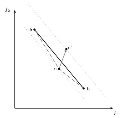
Figure 2: LB points $a$ and $b$, new “incumbent” point $c$, through cut generation lifted to $c^{\prime}$

4.2.3 Partial decomposition

Following Crainic et al., (2016), partial decomposition appears to be a viable option to obtain further speedups in the context of a Benders type algorithm. It refers to incorporating some of the scenarios into the master problem. Let $N^{*}$ denote the set of scenarios that are incorporated into the master LP, different strategies regarding which scenario should be part of $N^{*}$ can be envisaged. In the simplest case, the first scenario is put into $N^{*}$. After preliminary testing we decided to keep the scenario with lowest deviation from the average scenario, plus the $k$ scenarios with highest deviation.

5 Computational experiments

The previously described algorithms have been implemented using Python and Gurobi 8. The algorithms are run on a cluster with Xeon E5-2650v2 CPUs at 2.6 GHz. Each job is allocated 8 GB of memory and two hours of CPU effort. Multi-threading is disabled in Gurobi. In what follows, we first give an overview of the considered benchmark instances. Thereafter, we compare the different methods and we discuss the obtained results.

5.1 Benchmark instances

We use a set of 26 instances which are derived from real world data from the region of Thiès in western Senegal (for further details on these data we refer to Tricoire et al., (2012)). These instances feature between 9 and 29 vertices. Only 10 scenarios were used in Tricoire et al., (2012); we use 10, 50, 100, 200, 300, 400, 500, 600, 700, 800, 900 and 1000 scenarios for each instance. Scenarios are generated using a procedure similar to the one in Tricoire et al., (2012). Using more scenarios improves the quality of the approximation of the real situation but typically requires additional CPU effort.

5.2 Cut separation settings

We compare several settings:

• no decomposition: all constraints are considered explicitly in the master problem, no cuts are generated during the branch-and-bound algorithm,

• base: base L-shaped method. No partial decomposition, no valid inequalities, cuts are systematically generated when they are violated.

• partial decomposition: the scenario with lowest deviation from average is built in the master problem, as well as the 4 samples with highest deviation.

• valid inequalities: the valid inequalities described at the end of Section 4.2.1 are added to the master problem.

• incumbent cuts: cuts are generated systematically at the root node of the tree search, then only on incumbent solutions, as described in Section 4.2.2.

• incumbent cuts + valid inequalities: Both strategies are used.

We first compare all settings in terms of CPU effort. Since there are 6 settings, 26 instances and 12 sample sizes, there are 1872 runs to compare. For that reason we present performance profiles. A performance profile is a chart that compares the performance of various algorithms (Dolan and Moré,, 2002). The performance of a setting for a given instance is the ratio of the CPU effort required with this setting for this instance over the best known CPU effort for the same instance. The best performance achievable is always 1. On a performance profile, performance is indicated on the $x$-axis while the $y$-axis indicates the ratio of instances solved with at least that level of performance by a certain setting. If a certain setting does not converge in solving a given instance within the allotted CPU budget, then this setting does not provide a performance for that instance.

Figure 3 provides a comparison of the performance profiles of all six settings on all instances and all sample sizes.

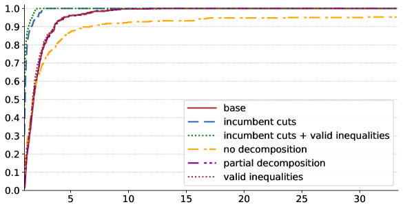
Figure 3: Performance profile: all settings on all test instances and all sample sizes.

The only setting that does not always converge using the CPU budget is no decomposition, thus already emphasizing the need for decomposition. We can also see that some settings are sometimes ten times slower than others. The two settings that only generate cuts on incumbent solutions appear to dominate the others.

For further insight, we now look at box plots for the same experimental data. We use the ggplot2 R package (Wickham,, 2016). Runs for which the algorithm does not converge are discarded. For the sake of readability, we only consider instances with at least 700 scenarios. This box plot is depicted in Figure 4.

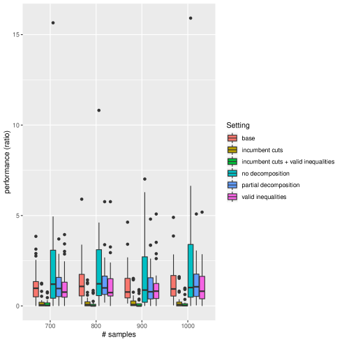
Figure 4: Box plot: all settings on all test instances, large sample sizes only.

We can now see that in certain cases, some methods are actually more than 15 times slower than the best method. It appears even more clearly that on large instances, which are the most interesting ones since they provide a better approximation of reality, settings generating cuts only for incumbent solutions perform better.

We now look at the two best settings only, in order to determine whether the valid inequalities provide any kind of significant improvement. For that purpose we first look at the performance profiles. They are depicted in Figure 5.

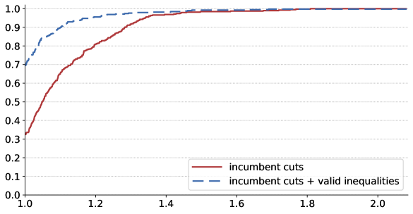
Figure 5: Performance profile: best settings on all test instances and all sample sizes.

The setting that includes valid inequalities is not always the best, as indicated by the fact that it does not start at 1. However, its curve is way above the one from the setting without valid inequalities, indicating a better performance overall. In general, neither setting offers any very bad performance.

We also provide a box plot for the two best settings in Figure 6.

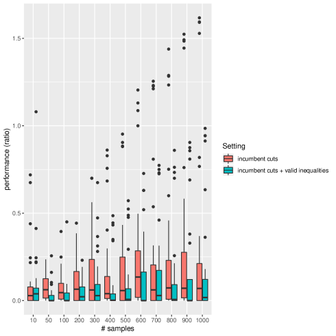
Figure 6: Box plot: best settings on all test instances and all sample sizes.

As we can see the worst performance is below 2, meaning than no setting is ever twice as slow as the best know setting. This, together with prior graphics, indicates that generating cuts only at incumbent solutions is the main cause of good performance. However, there is a clear trend in favor of the setting that also includes valid inequalities, observed for all sample sizes but the smallest (10).

Based on these observations, it is clear that the best setting is the one which both (i) only generates cuts at incumbent solutions and (ii) includes valid inequalities in the master problem, i.e. incumbent cuts + valid inequalities.

5.3 Benchmark data

In order to facilitate future comparisons, we provide detailed results on each instance for the overall best setting, which is incumbent cuts + valid inequalities. These results can be found in Appendix A.

6 Conclusions and outlook

We have defined a bi-objective facility location problem (BOSFLP), which considers both a deterministic objective (cost minimization) and a stochastic one (population coverage maximization), approximated using a sampling approach. The aim of the BOSFLP is to determine the set of efficient solutions using the Pareto approach, but aiming for good approximations with regard to the stochastic objective means considering large samples of random realizations, which makes standard approaches impractical. We decomposed the original problem and integrated Benders decomposition (L-shaped method) in a bi-objective branch-and-bound (BIOBAB) algorithm. This is, to the best of our knowledge, the first time that Benders decomposition has been integrated in a bi-objective branch-and-bound algorithm. Experiments show that the decomposition approach outperforms the explicit consideration of all samples in the original model.

We also implemented several known improvements to the L-shaped method, and adapted them to the bi-objective context. Among all settings, we observed that generating Benders cuts only at the root node and at integer solutions speeds up the search considerably. The developed strategy for integrating cutting plane generation into the lower bound set algorithm generalizes to any type of cut and thus paves the way for the development of general purpose bi-objective branch-and-cut algorithms relying on bound sets. We also observed that valid inequalities on bounds for sample-dependent values of the stochastic objective bring a significant improvement. In both cases, experimental observations were significant enough to justify making these recommendations permanent, at least in the context of the BOSFLP.

Research perspectives include the incorporation of additional enhancements into the L-shaped method. Crainic et al., (2016) propose to use more sophisticated partial decomposition strategies, such as the clustering-mean strategy in which similar scenarios are clustered and a good representative from each cluster is incorporated into the master program, or the convex hull strategy, where scenarios that include other scenarios in their convex hull are integrated in the master program. Magnanti and Wong, (1981) suggest improvements based on the notion of Pareto optimal cuts, a concept which has also been successfully employed by Adulyasak et al., (2015). The literature on the single-objective L-shaped method is abundant, and there are still lessons to be learnt in applying these techniques to the bi-objective context. Moreover, as illustrated by Tricoire et al., (2012), in the bi-objective context there is potential for improvements that rely on the interaction of the two objectives; one of our future goals is to develop bi-objective specific improvements for Benders decomposition techniques.

Acknowledgments

This work has been funded by the Austrian Science Fund (FWF): P31366 and P23589. This support is gratefully acknowledged.

Appendix A Benchmark results

We report benchmark results for the best setting, incumbent cuts + valid inequalities. Other settings may offer a better performance in some cases, but this is the setting that works best overall. Each table corresponds to a different sample size, and each table row provides indicators for one run. Indicators for each run are the number of vertices in the instance (vertices), the number of linear programs solved (LPs), the number of branch-and-bound nodes (B&B nodes), the number of cuts generated (cuts) and the CPU effort in seconds (CPU).

Instance	vertices	LPs	B&B nodes	cuts	CPU (s)
Ndiakhene	9	11	1	35	0.19
Cherif_Lo	10	143	21	78	0.44
Thienaba	10	122	33	56	0.35
Ndieyene_Shirak	11	164	25	92	0.52
Notto_Gouye_Diama	11	34	7	95	0.3
Malicounda_Wolof	12	16	1	48	0.24
Mbayene	12	220	41	69	0.56
Pekesse	12	68	7	92	0.4
Thiadiaye	13	25	3	77	0.31
Thilmanka	14	25	1	60	0.31
Mont_Roland	15	71	9	110	0.54
Sandira	15	32	5	80	0.37
Koul	16	245	39	126	0.86
Meouane	17	137	31	125	0.61
Neugeniene	17	130	11	129	0.75
Ndiass	18	25	1	148	0.58
Pire_Goureye	18	243	31	143	1.0
Merina_Dakhar	19	116	19	150	0.86
Ngandiouf	19	763	167	72	1.71
Nguekhokh	19	63	3	156	0.77
Touba_Toul	20	511	105	183	1.46
Tassette	21	425	79	252	1.75
Diender_Guedj	22	1075	197	271	2.91
Ndiagagniao	24	4632	1165	254	7.26
Notto	28	6311	1591	262	10.6
Pout	29	5391	1513	321	8.91

Table 1: Indicators for incumbent cuts + valid inequalities (10 samples).

Instance	vertices	LPs	B&B nodes	cuts	CPU (s)
Ndiakhene	9	10	1	105	0.34
Cherif_Lo	10	166	17	288	1.47
Thienaba	10	125	27	250	1.17
Ndieyene_Shirak	11	443	83	279	2.32
Notto_Gouye_Diama	11	19	3	191	0.66
Malicounda_Wolof	12	16	1	115	0.51
Mbayene	12	267	45	238	2.01
Pekesse	12	250	31	329	2.22
Thiadiaye	13	31	3	167	0.85
Thilmanka	14	25	1	125	0.75
Mont_Roland	15	167	31	256	1.6
Sandira	15	67	17	179	1.3
Koul	16	205	31	296	2.69
Meouane	17	75	9	317	2.31
Neugeniene	17	115	11	362	2.78
Ndiass	18	170	39	359	2.46
Pire_Goureye	18	322	67	369	4.25
Merina_Dakhar	19	504	115	313	3.76
Ngandiouf	19	357	67	252	4.23
Nguekhokh	19	83	3	321	2.93
Touba_Toul	20	968	203	541	7.54
Tassette	21	349	51	481	6.16
Diender_Guedj	22	1131	231	678	9.62
Ndiagagniao	24	3549	901	802	20.21
Notto	28	10613	2733	928	55.29
Pout	29	4640	1205	721	24.47

Table 2: Indicators for incumbent cuts + valid inequalities (50 samples).

Instance	vertices	LPs	B&B nodes	cuts	CPU (s)
Ndiakhene	9	11	1	185	0.52
Cherif_Lo	10	166	15	557	3.11
Thienaba	10	125	27	462	2.21
Ndieyene_Shirak	11	306	63	601	4.34
Notto_Gouye_Diama	11	53	11	307	1.41
Malicounda_Wolof	12	16	1	250	0.9
Mbayene	12	216	31	367	3.18
Pekesse	12	110	13	626	2.96
Thiadiaye	13	46	7	370	1.89
Thilmanka	14	24	1	267	1.42
Mont_Roland	15	487	99	651	4.67
Sandira	15	37	5	311	2.01
Koul	16	228	37	678	5.76
Meouane	17	147	23	542	4.79
Neugeniene	17	232	31	597	6.12
Ndiass	18	213	49	700	6.2
Pire_Goureye	18	412	93	783	8.85
Merina_Dakhar	19	465	101	571	7.12
Ngandiouf	19	289	57	464	8.47
Nguekhokh	19	418	71	810	9.77
Touba_Toul	20	2040	437	1082	20.34
Tassette	21	179	19	834	9.15
Diender_Guedj	22	1062	219	1197	20.11
Ndiagagniao	24	3231	817	1454	39.72
Notto	28	15976	4073	1695	141.32
Pout	29	6290	1659	1486	62.84

Table 3: Indicators for incumbent cuts + valid inequalities (100 samples).

Instance	vertices	LPs	B&B nodes	cuts	CPU (s)
Ndiakhene	9	11	1	454	1.19
Cherif_Lo	10	191	17	1127	7.04
Thienaba	10	139	25	781	4.48
Ndieyene_Shirak	11	199	39	825	6.94
Notto_Gouye_Diama	11	20	3	580	2.37
Malicounda_Wolof	12	17	1	405	1.88
Mbayene	12	252	43	745	7.67
Pekesse	12	392	61	1401	9.73
Thiadiaye	13	33	3	537	3.26
Thilmanka	14	25	1	488	3.34
Mont_Roland	15	650	141	1471	12.47
Sandira	15	70	15	574	5.16
Koul	16	423	79	1445	14.95
Meouane	17	145	19	931	9.03
Neugeniene	17	242	33	1105	12.35
Ndiass	18	308	77	1180	13.19
Pire_Goureye	18	720	155	1618	21.44
Merina_Dakhar	19	560	127	1135	15.81
Ngandiouf	19	364	71	843	19.1
Nguekhokh	19	471	97	1473	18.5
Touba_Toul	20	1419	275	2316	40.58
Tassette	21	319	53	1567	23.5
Diender_Guedj	22	2232	463	2598	63.0
Ndiagagniao	24	4238	1125	1806	69.05
Notto	28	12136	3121	2686	217.35
Pout	29	5609	1469	2739	115.0

Table 4: Indicators for incumbent cuts + valid inequalities (200 samples).

Instance	vertices	LPs	B&B nodes	cuts	CPU (s)
Ndiakhene	9	11	1	630	1.62
Cherif_Lo	10	181	23	1385	10.43
Thienaba	10	172	35	1281	5.48
Ndieyene_Shirak	11	343	45	1579	14.72
Notto_Gouye_Diama	11	16	1	984	3.48
Malicounda_Wolof	12	17	1	595	2.78
Mbayene	12	211	31	981	9.13
Pekesse	12	295	43	1611	12.07
Thiadiaye	13	47	7	1025	6.16
Thilmanka	14	25	1	620	4.98
Mont_Roland	15	577	115	1683	17.02
Sandira	15	56	11	931	7.73
Koul	16	416	79	1745	20.66
Meouane	17	242	41	1419	16.26
Neugeniene	17	209	25	1573	20.51
Ndiass	18	511	113	2200	26.37
Pire_Goureye	18	396	65	1784	28.09
Merina_Dakhar	19	461	111	1626	25.53
Ngandiouf	19	342	61	1123	26.73
Nguekhokh	19	285	57	1868	23.96
Touba_Toul	20	1877	377	3125	69.57
Tassette	21	255	33	2104	32.76
Diender_Guedj	22	2077	417	3506	104.28
Ndiagagniao	24	5820	1409	4107	205.17
Notto	28	9836	2497	3624	302.43
Pout	29	6867	1829	4184	212.21

Table 5: Indicators for incumbent cuts + valid inequalities (300 samples).

Instance	vertices	LPs	B&B nodes	cuts	CPU (s)
Ndiakhene	9	11	1	720	2.12
Cherif_Lo	10	103	9	1832	11.16
Thienaba	10	145	29	1649	11.08
Ndieyene_Shirak	11	208	29	1968	14.97
Notto_Gouye_Diama	11	16	1	1055	4.35
Malicounda_Wolof	12	17	1	926	4.71
Mbayene	12	293	55	1415	17.67
Pekesse	12	278	27	2603	21.68
Thiadiaye	13	32	3	1319	7.89
Thilmanka	14	25	1	921	7.47
Mont_Roland	15	516	105	2108	23.31
Sandira	15	64	13	1266	11.55
Koul	16	391	77	2486	29.5
Meouane	17	208	35	1815	20.94
Neugeniene	17	165	23	2400	26.68
Ndiass	18	667	157	2731	39.02
Pire_Goureye	18	515	103	2665	39.09
Merina_Dakhar	19	698	163	2205	35.16
Ngandiouf	19	601	115	1633	45.38
Nguekhokh	19	420	109	2604	36.78
Touba_Toul	20	1752	347	5580	110.54
Tassette	21	290	37	2809	50.14
Diender_Guedj	22	1172	241	4265	99.05
Ndiagagniao	24	3502	835	4297	184.15
Notto	28	15150	3825	7627	724.75
Pout	29	7215	1903	6584	337.43

Table 6: Indicators for incumbent cuts + valid inequalities (400 samples).

Instance	vertices	LPs	B&B nodes	cuts	CPU (s)
Ndiakhene	9	11	1	870	2.84
Cherif_Lo	10	109	11	2375	16.8
Thienaba	10	215	41	1962	14.68
Ndieyene_Shirak	11	689	143	3782	35.66
Notto_Gouye_Diama	11	35	7	1325	7.6
Malicounda_Wolof	12	17	1	999	5.44
Mbayene	12	178	33	1561	16.44
Pekesse	12	386	53	3319	31.52
Thiadiaye	13	160	33	2400	14.45
Thilmanka	14	24	1	1265	8.8
Mont_Roland	15	632	131	3226	35.6
Sandira	15	66	13	1491	13.3
Koul	16	411	75	3569	49.5
Meouane	17	187	33	2325	28.24
Neugeniene	17	225	27	2836	40.15
Ndiass	18	465	139	2943	42.23
Pire_Goureye	18	707	151	3290	53.78
Merina_Dakhar	19	687	149	2490	41.37
Ngandiouf	19	746	159	1844	57.26
Nguekhokh	19	765	199	3464	55.49
Touba_Toul	20	1446	293	5629	125.24
Tassette	21	203	29	3100	46.08
Diender_Guedj	22	2549	545	6222	219.84
Ndiagagniao	24	3175	811	4359	216.4
Notto	28	10300	2627	7026	677.45
Pout	29	9699	2615	7750	531.69

Table 7: Indicators for incumbent cuts + valid inequalities (500 samples).

Instance	vertices	LPs	B&B nodes	cuts	CPU (s)
Ndiakhene	9	11	1	1000	3.22
Cherif_Lo	10	194	21	2697	26.34
Thienaba	10	243	59	2480	15.39
Ndieyene_Shirak	11	377	57	3911	40.69
Notto_Gouye_Diama	11	25	3	1627	7.89
Malicounda_Wolof	12	16	1	1200	6.12
Mbayene	12	286	59	1856	21.41
Pekesse	12	117	11	3329	24.19
Thiadiaye	13	46	7	1991	13.96
Thilmanka	14	25	1	1340	10.53
Mont_Roland	15	766	161	4389	56.04
Sandira	15	68	13	1811	13.83
Koul	16	370	69	4140	55.05
Meouane	17	269	47	2951	42.71
Neugeniene	17	170	17	3262	51.38
Ndiass	18	468	113	3462	53.77
Pire_Goureye	18	736	149	3864	81.04
Merina_Dakhar	19	630	141	3022	53.24
Ngandiouf	19	343	65	2549	68.44
Nguekhokh	19	893	225	4289	81.24
Touba_Toul	20	1410	237	7485	185.48
Tassette	21	359	55	3737	76.48
Diender_Guedj	22	1747	383	6754	197.8
Ndiagagniao	24	4169	1085	6062	348.91
Notto	28	10196	2545	7830	824.91
Pout	29	5767	1547	7242	417.66

Table 8: Indicators for incumbent cuts + valid inequalities (600 samples).

Instance	vertices	LPs	B&B nodes	cuts	CPU (s)
Ndiakhene	9	11	1	1416	4.94
Cherif_Lo	10	199	21	3102	30.55
Thienaba	10	191	39	2310	22.69
Ndieyene_Shirak	11	395	69	4471	44.67
Notto_Gouye_Diama	11	23	3	1804	7.97
Malicounda_Wolof	12	16	1	2105	9.5
Mbayene	12	192	25	2385	29.63
Pekesse	12	241	35	4197	37.8
Thiadiaye	13	49	7	2341	15.59
Thilmanka	14	24	1	1745	13.53
Mont_Roland	15	634	127	4459	55.65
Sandira	15	61	13	2272	20.31
Koul	16	472	93	4649	73.74
Meouane	17	148	23	3526	37.49
Neugeniene	17	338	59	3648	60.13
Ndiass	18	609	141	4299	82.22
Pire_Goureye	18	620	121	4307	81.37
Merina_Dakhar	19	1046	249	4454	88.32
Ngandiouf	19	418	73	2874	81.81
Nguekhokh	19	1112	281	5363	94.39
Touba_Toul	20	3078	677	7367	254.06
Tassette	21	365	61	4757	90.2
Diender_Guedj	22	1862	393	7655	271.29
Ndiagagniao	24	3690	937	6732	362.6
Notto	28	12753	3273	9053	1153.8
Pout	29	8741	2339	12372	892.39

Table 9: Indicators for incumbent cuts + valid inequalities (700 samples).

Instance	vertices	LPs	B&B nodes	cuts	CPU (s)
Ndiakhene	9	11	1	1390	4.67
Cherif_Lo	10	214	23	4416	37.43
Thienaba	10	182	37	2525	20.82
Ndieyene_Shirak	11	253	43	4035	36.19
Notto_Gouye_Diama	11	45	9	2249	12.34
Malicounda_Wolof	12	17	1	1615	8.8
Mbayene	12	219	37	2676	35.43
Pekesse	12	103	13	3857	29.22
Thiadiaye	13	49	7	2735	19.43
Thilmanka	14	24	1	1580	14.12
Mont_Roland	15	582	113	4445	58.15
Sandira	15	83	17	2110	24.33
Koul	16	472	91	5776	93.74
Meouane	17	237	39	3863	58.61
Neugeniene	17	258	39	3767	75.57
Ndiass	18	330	85	4427	66.73
Pire_Goureye	18	554	111	4735	80.23
Merina_Dakhar	19	357	73	3849	63.43
Ngandiouf	19	572	107	3332	103.31
Nguekhokh	19	784	223	5581	93.88
Touba_Toul	20	2121	427	8548	258.43
Tassette	21	297	39	5746	110.27
Diender_Guedj	22	2298	487	8687	351.12
Ndiagagniao	24	4547	1109	9431	548.11
Notto	28	14639	3699	11121	1522.24
Pout	29	5104	1275	10398	651.21

Table 10: Indicators for incumbent cuts + valid inequalities (800 samples).

Instance	vertices	LPs	B&B nodes	cuts	CPU (s)
Ndiakhene	9	11	1	1555	5.21
Cherif_Lo	10	117	11	3715	34.87
Thienaba	10	228	49	3486	30.81
Ndieyene_Shirak	11	385	67	4937	51.89
Notto_Gouye_Diama	11	63	13	2352	14.58
Malicounda_Wolof	12	17	1	2135	10.49
Mbayene	12	295	59	3287	42.85
Pekesse	12	315	45	4949	54.64
Thiadiaye	13	43	7	3120	22.09
Thilmanka	14	25	1	2040	17.46
Mont_Roland	15	906	201	7784	113.98
Sandira	15	77	17	2643	27.51
Koul	16	448	87	5799	102.2
Meouane	17	292	53	4488	76.73
Neugeniene	17	245	35	5181	85.7
Ndiass	18	554	129	6010	108.32
Pire_Goureye	18	446	81	6068	123.23
Merina_Dakhar	19	561	113	4709	107.37
Ngandiouf	19	474	87	3664	107.18
Nguekhokh	19	520	151	5168	89.1
Touba_Toul	20	2233	449	12664	380.63
Tassette	21	489	85	5656	134.4
Diender_Guedj	22	2848	617	11535	492.3
Ndiagagniao	24	4065	1009	10882	642.0
Notto	28	9397	2361	11463	1171.44
Pout	29	7902	2129	14670	1056.83

Table 11: Indicators for incumbent cuts + valid inequalities (900 samples).

Instance	vertices	LPs	B&B nodes	cuts	CPU (s)
Ndiakhene	9	11	1	1725	5.56
Cherif_Lo	10	123	17	5043	40.84
Thienaba	10	172	35	3807	34.49
Ndieyene_Shirak	11	288	51	6377	62.43
Notto_Gouye_Diama	11	20	3	2491	12.72
Malicounda_Wolof	12	16	1	2190	11.7
Mbayene	12	305	59	3728	39.78
Pekesse	12	154	15	5669	46.5
Thiadiaye	13	268	59	5460	40.66
Thilmanka	14	25	1	2445	20.35
Mont_Roland	15	808	169	7302	106.04
Sandira	15	59	13	2846	29.49
Koul	16	408	79	6350	108.44
Meouane	17	277	51	5350	83.05
Neugeniene	17	182	23	4886	81.65
Ndiass	18	332	87	5734	88.5
Pire_Goureye	18	559	113	6854	138.85
Merina_Dakhar	19	448	91	4683	85.16
Ngandiouf	19	660	139	4171	129.67
Nguekhokh	19	717	199	6110	121.03
Touba_Toul	20	1845	397	8545	292.24
Tassette	21	305	51	7060	154.45
Diender_Guedj	22	1714	385	10891	389.12
Ndiagagniao	24	3906	915	11495	793.63
Notto	28	13451	3429	13171	2019.97
Pout	29	7246	1965	15670	1159.21

Table 12: Indicators for incumbent cuts + valid inequalities (1000 samples).

References

- Abdelaziz, (2012) Abdelaziz, F. B. (2012). Solution approaches for the multiobjective stochastic programming. European Journal of Operational Research, 216(1):1 – 16.
- Adulyasak et al., (2015) Adulyasak, Y., Cordeau, J.-F., and Jans, R. (2015). Benders decomposition for production routing under demand uncertainty. Operations Research, 63(4):851–867.
- Aneja and Nair, (1979) Aneja, Y. P. and Nair, K. P. K. (1979). Bicriteria transportation problem. Management Science, 25:73–78.
- Benders, (1962) Benders, J. F. (1962). Partitioning procedures for solving mixed-variables programming problems. Numerische mathematik, 4(1):238–252.
- Bhaskaran and Turnquist, (1990) Bhaskaran, S. and Turnquist, M. A. (1990). Multiobjective transportation considerations in multiple facility location. Transportation Research Part A: General, 24(2):139–148.
- Birge and Louveaux, (2011) Birge, J. R. and Louveaux, F. (2011). Introduction to stochastic programming. Springer Science & Business Media.
- Caballero et al., (2004) Caballero, R., Cerda, E., Muos, M., and Rey, L. (2004). Stochastic approach versus multiobjective approach for obtaining efficient solutions in stochastic multiobjective programming problems. European Journal of Operational Research, 158:633–648.
- Cardona-Valdés et al., (2011) Cardona-Valdés, Y., Álvarez, A., and Ozdemir, D. (2011). A bi-objective supply chain design problem with uncertainty. Transportation Research Part C, 19:821–832.
- Church and ReVelle, (1974) Church, R. and ReVelle, C. R. (1974). The maximal covering location problem. Papers in regional science, 32(1):101–118.
- Crainic et al., (2016) Crainic, T. G., Rei, W., Hewitt, M., and Maggioni, F. (2016). Partial benders decomposition strategies for two-stage stochastic integer programs. Technical report, Technical Report 37, CIRRELT.
- Current and Schilling, (1994) Current, J. R. and Schilling, D. A. (1994). The median tour and maximal covering tour problems: Formulations and heuristics. European Journal of Operational Research, 73(1):114–126.
- Doerner et al., (2007) Doerner, K., Focke, A., and Gutjahr, W. J. (2007). Multicriteria tour planning for mobile healthcare facilities in a developing country. European Journal of Operational Research, 179(3):1078–1096.
- Dolan and Moré, (2002) Dolan, E. D. and Moré, J. J. (2002). Benchmarking optimization software with performance profiles. Mathematical Programming, 91(2):201–213.
- Ehrgott, (2005) Ehrgott, M. (2005). Multicriteria Optimization. Springer Berlin Heidelberg.
- Ehrgott and Gandibleux, (2006) Ehrgott, M. and Gandibleux, X. (2006). Bound sets for biobjective combinatorial optimization problems. Computers & Operations Research, 34:2674–2694.
- Elçi and Noyan, (2018) Elçi, Ö. and Noyan, N. (2018). A chance-constrained two-stage stochastic programming model for humanitarian relief network design. Transportation research part B: methodological, 108:55–83.
- Farahani et al., (2010) Farahani, R. Z., SteadieSeifi, M., and Asgari, N. (2010). Multiple criteria facility location problems: A survey. Applied Mathematical Modelling, 34(7):1689–1709.
- Fonseca et al., (2010) Fonseca, M., García-Sánchez, A., Ortega-Mier, M., and Saldanha da Gama, F. (2010). A stochastic bi-objective location model for strategic reverse logistics. TOP, 18:158–184.
- Grass and Fischer, (2016) Grass, E. and Fischer, K. (2016). Two-stage stochastic programming in disaster management: A literature survey. Surveys in Operations Research and Management Science, 21(2):85–100.
- Gutjahr and Dzubur, (2016) Gutjahr, W. J. and Dzubur, N. (2016). Bi-objective bilevel optimization of distribution center locations considering user equilibria. Transportation Research Part E: Logistics and Transportation Review, 85:1 – 22.
- Gutjahr and Nolz, (2016) Gutjahr, W. J. and Nolz, P. C. (2016). Multicriteria optimization in humanitarian aid. European Journal of Operational Research, 252(2):351–366.
- Gutjahr and Pichler, (2016) Gutjahr, W. J. and Pichler, A. (2016). Stochastic multi-objective optimization: a survey on non-scalarizing methods. Annals of Operations Research, 236:475–499.
- Hamacher and Drezner, (2002) Hamacher, H. W. and Drezner, Z. (2002). Facility location: applications and theory. Springer Science & Business Media.
- Harewood et al., (2002) Harewood, S. et al. (2002). Emergency ambulance deployment in barbados: a multi-objective approach. Journal of the Operational Research Society, 53(2):185–192.
- Jozefowiez et al., (2007) Jozefowiez, N., Semet, F., and Talbi, E.-G. (2007). The bi-objective covering tour problem. Computers & operations research, 34(7):1929–1942.
- Khorsi et al., (2013) Khorsi, M., Bozorgi-Amiri, A., and Ashjari, B. (2013). A nonlinear dynamic logistics model for disaster response under uncertainty. significance, 3:4.
- Magnanti and Wong, (1981) Magnanti, T. L. and Wong, R. T. (1981). Accelerating benders decomposition: Algorithmic enhancement and model selection criteria. Operations research, 29(3):464–484.
- Nolz et al., (2010) Nolz, P. C., Doerner, K. F., Gutjahr, W. J., and Hartl, R. F. (2010). A bi-objective metaheuristic for disaster relief operation planning. In Advances in multi-objective nature inspired computing, pages 167–187. Springer.
- Parragh and Tricoire, (2019) Parragh, S. N. and Tricoire, F. (2019). Branch-and-bound for bi-objective integer programming. INFORMS Journal on Computing.
- Rath et al., (2016) Rath, S., Gendreau, M., and Gutjahr, W. J. (2016). Bi-objective stochastic programming models for determining depot locations in disaster relief operations. International Transactions in Operational Research, 23(6):997–1023.
- Stidsen et al., (2014) Stidsen, T., Andersen, K. A., and Dammann, B. (2014). A branch and bound algorithm for a class of biobjective mixed integer programs. Management Science, 60(4):1009–1032.
- Tomasini and Van Wassenhove, (2009) Tomasini, R. M. and Van Wassenhove, L. N. (2009). From preparedness to partnerships: case study research on humanitarian logistics. International Transactions in operational research, 16(5):549–559.
- Tricoire et al., (2012) Tricoire, F., Graf, A., and Gutjahr, W. (2012). The bi-objective stochastic covering tour problem. Computers & Operations Research, 39:1582–1592.
- Van Slyke and Wets, (1969) Van Slyke, R. and Wets, R. (1969). L-shaped linear programs with applications to optimal control and stochastic programming. SIAM Journal on Applied Mathematics, pages 638–663.
- Villegas et al., (2006) Villegas, J. G., Palacios, F., and Medaglia, A. L. (2006). Solution methods for the bi-objective (cost-coverage) unconstrained facility location problem with an illustrative example. Annals of Operations Research, 147(1):109–141.
- Wickham, (2016) Wickham, H. (2016). ggplot2: Elegant Graphics for Data Analysis. Springer-Verlag New York.