Federated Stochastic Gradient Langevin Dynamics

Abstract

Stochastic gradient MCMC methods, such as stochastic gradient Langevin dynamics (SGLD), employ fast but noisy gradient estimates to enable large-scale posterior sampling. Although we can easily extend SGLD to distributed settings, it suffers from two issues when applied to federated non-IID data. First, the variance of these estimates increases significantly. Second, delaying communication causes the Markov chains to diverge from the true posterior even for very simple models. To alleviate both these problems, we propose conducive gradients, a simple mechanism that combines local likelihood approximations to correct gradient updates. Notably, conducive gradients are easy to compute, and since we only calculate the approximations once, they incur negligible overhead. We apply conducive gradients to distributed stochastic gradient Langevin dynamics (DSGLD) and call the resulting method federated stochastic gradient Langevin dynamics (FSGLD). We demonstrate that our approach can handle delayed communication rounds, converging to the target posterior in cases where DSGLD fails. We also show that FSGLD outperforms DSGLD for non-IID federated data with experiments on metric learning and neural networks.

1 Introduction

Gradient-based Markov Chain Monte Carlo (MCMC) methods are the de facto standard to sample from Bayesian posteriors. However, computing gradients exactly can be prohibitive even for moderately large data sets. Following the success of stochastic gradients in large-scale optimization and inspired by [Welling and Teh, 2011], many MCMC algorithms were adapted to leverage fast but noisy gradient evaluations computed on mini-batches of data [Ma et al., 2015]. Examples include stochastic gradient Langevin dynamics (SGLD) [Welling and Teh, 2011], stochastic gradient Hamiltonian Monte Carlo (SGHMC) [Chen et al., 2014], and Riemann manifold Hamiltonian Monte Carlo (RMHMC) [Girolami and Calderhead, 2011]. These methods have established themselves as popular choices for scalable Bayesian inference.

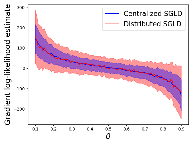
Figure 1: Comparison between gradient estimators using centralized (SGLD) and distributed data (DSGLD), for a model with Bernoulli likelihood and uniform prior. We computed gradients using 5 samples from a total of 30 observations generated from fair coin tosses. For DSGLD, we simulate the federated non-IID regime splitting data between 3 equally-available shards of same size but distinct means – $0.1$, $0.5$ and $0.9$. The confidence bars reflect one standard deviation. DSGLD (red) shows higher variance than SGLD (blue) even for this simple case.

Complementary to data subsampling, which underlies the use of stochastic gradients, we can also split data across several workers and use distributed computations to scale up MCMC [Neiswanger et al., 2014, Scott et al., 2016, Terenin et al., 2020, Wang et al., 2015, Nemeth and Sherlock, 2018, Mesquita et al., 2019]. In particular, Ahn et al. [2014] extend stochastic gradient MCMC using a simple estimator that accounts for data partitions and propose distributed SGLD (DSGLD). More specifically, DSGLD operates passing a Markov chain between computing nodes and using only local data to estimate gradients at each step. The gradient estimates are then scaled accordingly to correct the bias.

Despite the popularity of stochastic gradient MCMC, no work has considered applications to federated learning. Notably, federated data arise independently in different clients/devices, and communication or privacy constraints prevent it from being disclosed to a server. As a consequence, data are often partitioned in a non-IID fashion. We argue that distributed methods such as vanilla DSGLD are inappropriate for the non-IID regime. In practice, this regime significantly amplifies the variance of stochastic gradients. Figure 1 illustrates this phenomenon for a simple model with Bernoulli likelihood. In turn, this can lead to poor mixing rates and slow convergence[Dubey et al., 2016]. Additionally, in federated settings, we want to avoid frequent communication, which can introduce bias and cause DSGLD to diverge from the target posterior [Ahn et al., 2014].

To mitigate these problems, we propose conducive gradients, a zero-mean stochastic function that aggregates approximations of each client’s likelihood factor. These approximations are computed independently on the client-side before and communicated only once. We add our conducive gradient to the gradient estimator proposed by Ahn et al. [2014] to derive a novel method, which we call federated stochastic gradient Langevin dynamics (FSGLD). We demonstrate that i) FSGLD converges to the true posterior in cases where DSGLD fails, and ii) FSGLD outperforms DSGLD in federated non-IID scenarios.

In general, we can compute conducive gradients in constant time and, since we compute the local approximations only once, FSGLD has the same computational complexity as DSGLD. We also provide convergence bounds for FSGLD and use these results to gain insight regarding how to efficiently choose local likelihood approximations which minimize the bound. Furthermore, we provide analysis for DSGLD since no formal analysis is available in the literature. There are well-established analyses of convergence for SGLD in serial settings[Chen et al., 2015, Nagapetyan et al., 2017, Baker et al., 2019, Teh et al., 2016, Vollmer et al., 2016], which we use as a starting point due to their relatively straightforward formulation.

We organize the remainder of this work as follows. In Section 2, we establish the notation and provide a brief review of serial and distributed SGLD. In Section 3, we introduce the concept of conducive gradients and use it to derive a novel SGLD algorithm tailored to federated data. In Section 4, we show convergence bounds for both our method and DSGLD. In Section 5, we show experimental results. Finally, we discuss related work in Section 6 and draw conclusions in Section 7.

2 Background and notation

Let $\mathbf{x}=\{x_{1},\ldots,x_{N}\}$ be a data set of size $N$ and let $p(\theta|\mathbf{x})\propto p(\theta)\prod_{i=1}^{N}p(x_{i}|\theta)$ be the density of a posterior distribution from which we wish to draw samples. Langevin dynamics [Neal, 2011] is a family of MCMC methods which utilizes the gradient of the log-posterior,

$$\nabla\log p(\theta|\mathbf{x})=\nabla\log p(\theta)+\sum_{i=1}^{N}\nabla\log p(x_{i}|\theta),$$

to generate proposals in a Metropolis-Hastings sampling scheme. For large data sets, computing the gradient of the log-likelihood with respect to the entire data set $\mathbf{x}$ becomes expensive. To mitigate this problem, stochastic gradient Langevin dynamics (SGLD) [Welling and Teh, 2011] uses stochastic gradients to approximate the full-data gradient.

Denoting by $\nabla\log p(\mathbf{x}^{(m)}|\theta_{t})=\sum_{x\in\mathbf{x}^{(m)}}\nabla\log p(x|\theta_{t})$ the gradient of the log-likelihood with respect to a minibatch $\mathbf{x}^{(m)}$ of size $m$, SGLD draws samples from the target distribution using a stochastic gradient update of the form

$$\theta_{t+1}=\theta_{t}+\frac{h_{t}}{2}v(\theta_{t})+\eta_{t},$$ (1)

in which $h_{t}$ is the step size, $\eta_{t}$ is a noise variable sampled from $\mathcal{N}(0,h_{t}I)$ and where

$$v(\theta_{t})=\nabla\log p(\theta_{t})+\frac{N}{m}\nabla\log p(\mathbf{x}^{(m)}|\theta_{t}).$$ (2)

In theory, step size is annealed according to a schedule satisfying $\sum_{t=1}^{\infty}h_{t}=\infty$ and $\sum_{t=1}^{\infty}h_{t}^{2}<\infty$. Note that as $h_{t}\rightarrow 0$, the Metropolis-Hastings acceptance rate goes asymptotically to one and thus, the accept-reject step is typically ignored in SGLD. While a proper annealing schedule yields an asymptotically exact algorithm, constant step sizes are commonly used in practice.

2.1 DSGLD

Ahn et al. [2014] propose DSGLD as an extension of SGLD to distributed settings (DSGLD), where we find data $\mathbf{x}$ to be partitioned into $S$ non-overlapping shards $\mathbf{x}_{s}$, each held by a client, such that $\mathbf{x}=\{\mathbf{x}_{1},\ldots,\mathbf{x}_{S}\}$. More specifically, DSGLD uses a modified version of the update in Equation 1 which is better suited for distributed data. The main idea is that in each iteration, a mini-batch is sampled within a shard, say $\mathbf{x}_{s}$, and the shard itself is sampled by a scheduler with probability $f_{s}$, with $\sum_{s=1}^{S}f_{s}=1$ and $f_{s}>0$ for all $s$. This results in the update

$$\theta_{t+1}=\theta_{t}+\frac{h_{t}}{2}v_{s_{t}}(\theta_{t})+\eta_{t},$$ (3)

in which $v$ is an unbiased gradient estimator given by

$$v_{s_{t}}(\theta_{t})=\nabla\log p(\theta_{t})+\frac{N_{s_{t}}}{f_{s_{t}}m}\nabla\log p(\mathbf{x}_{s_{t}}^{(m)}|\theta_{t}),$$ (4)

and where $N_{s_{t}}$ denotes the size of shard $\mathbf{x}_{s_{t}}$, chosen at time $t$. Intuitively, if a mini-batch of $m$ data points is chosen uniformly at random from $\mathbf{x}_{s_{t}}$, then $N_{s_{t}}/m$ scales $\nabla\log p(\mathbf{x}_{s_{t}}^{(m)}|\theta_{t})$ to be an unbiased estimator for $\nabla\log p(\mathbf{x}_{s_{t}}|\theta_{t})$ , while $f_{s_{t}}^{-1}$ further scales this gradient to be an unbiased estimator for $\nabla\log p(\mathbf{x}|\theta_{t})$.

A downside of this approach is the constant communication between workers. To alleviate this problem, Ahn et al. [2014] propose taking multiple update steps within the same shard before moving to another worker. Nonetheless, this reduction in communication costs comes at the expense of some loss in asymptotic accuracy. It is worth noting that, while the data are distributed, we can still understand DSGLD chains as entirely serial procedures. In practice, however, distributed settings are naturally amenable to running multiple chains in parallel.

3 FSGLD: Federated inference using conducive gradients

In DSGLD, stochastic gradient updates are computed on mini-batches sampled within the data shard of a specific client, which adds bias to the updates and increases variance globally. This is especially significant if for non-IID federated data, when shards are heterogeneous and likelihood contributions vastly differ between two devices. To counteract this, we would like to make the local updates benefit from other shards’ information, ideally without significantly increasing either computational cost or memory requirements. Our strategy to achieve this goal is to augment the local updates, in Equation 3, with an auxiliary gradient computed on a tractable surrogate for the full-data likelihood $p(\mathbf{x}|\theta)$.

We assume here that the surrogate, denoted as $q(\theta)$, factorizes over shards, such as $q(\theta)=\prod_{s}q_{s}(\theta)$, where each $q_{s}(\theta)$ is itself a surrogate for $p(\mathbf{x}_{s}|\theta)$, i.e. the likelihood w.r.t. an entire shard $s$. Given these surrogates, we define the conducive gradient w.r.t. shard $s$ as

$$g_{s}(\theta) =\nabla\log q(\theta)-\frac{1}{f_{s}}\nabla\log q_{s}(\theta).$$

Using the conducive gradient $g_{s}$ we define our novel update rule as

$$\begin{split}\theta_{t+1}=\theta_{t}&+\frac{h_{t}}{2}\bigg{(}v_{s_{t}}(\theta_{t})+g_{s_{t}}(\theta_{t})\bigg{)}+\eta_{t}.\end{split}$$ (5)

Algorithm 1 describes our method, federated stochastic Langevin dynamics (FSGLD). We discuss the validity of our novel gradient estimator ($v_{s}+g_{s}$) in Section 4.

Remark 1 (Controlling exploration).

Note that conducive gradients can alternatively be written as

$$g_{s}(\theta)=\nabla\log\frac{q(\theta)}{q_{s}(\theta)^{f_{s}^{-1}}},$$ (6)

making it explicit that these terms encourage the exploration of regions in which we believe, based on the approximations $q$ and $q_{s}$, the posterior density to be high but the density within shard $s$ to be low. We can explicitly control the extent of this exploration by multiplying the conducive gradient by a constant $\alpha>0$ to obtain the modified gradient estimator:

$$\frac{N_{s}}{f_{s}m}\nabla\log p(\mathbf{x}_{s}^{(m)}|\theta)+\alpha g_{s}(\theta).$$ (7)

Algorithm 1 FSGLD

Client-side Update($T$, $\theta_{0}$, $s$)

Given: Total number of iterations $T$, step sizes $\{h_{t}\}_{t=0}^{T-1}$, initial chain state $\theta_{0}$, client number $s$.

for  $t=0\ldots T-1$ do

     Sample a mini-batch $\mathbf{x}_{s}^{(m)}$ of size $m$ from $\mathbf{x}_{s}$

     $d_{s}\leftarrow\nabla\log p(\theta)+\frac{1}{f_{s}}\frac{N_{s}}{m}\nabla\log p(\mathbf{x}_{s}^{(m)}|\theta)$ $\triangleright$ DSGLD estimator

     $g_{s}\leftarrow-\frac{1}{f_{s}}\nabla\log q_{s}(\theta)+\nabla\log q(\theta)$ $\triangleright$ Conducive gradient

     $\theta_{t+1}\leftarrow\theta_{t}+\frac{h_{t}}{2}(d_{s}+g_{s})+\eta_{t}$ $\triangleright$ According to Eq. (5) end for

Reassign_chain($\theta_{0},\ldots,\theta_{T}$) $\triangleright$ Send chain to server

Server-side Reassign_chain($\theta_{0},\ldots,\theta_{T}$)

Given: Client probabilities $f_{1},\ldots,f_{S}$.

Store the received chain

$c\sim\texttt{Categorical}(f_{1},\ldots,f_{S})$ $\triangleright$ Choose a client at random.

Update($T$, $\theta_{T}$, $c$) $\triangleright$ Pass on chain to client $c$.

3.1 Choice of surrogates $q_{1},\ldots,q_{S}$

The key idea in choosing $q_{s}$ is to obtain an approximation of $p(\mathbf{x}_{s}|\theta)$ with a parametric form, and to choose the parametric form such that $\nabla\log q_{s}(\theta)$ computation is inexpensive. It is particularly beneficial if the gradient can be computed in a single gradient evaluation instead of iterating over all data, of size $N_{s}$, of said shard $s$. Exponential family distributions are especially convenient for this purpose, as they are closed under product operations, enabling us to compute $\nabla\log q(\theta_{t})$ in a single gradient evaluation. This keeps the additional cost of our method negligible even when $S\gg m$. More specifically, with exponential family surrogates, this cost is constant with respect to the number of clients $S$.

In this work, we use a simulation-based approach to compute $q_{s}$ by first drawing from $p_{s}\propto p(\mathbf{x}_{s}|\theta)$ locally employing SGLD, and using the resulting samples to compute the parameters of an exponential family approximation. To avoid communication overhead, $q_{1},\ldots,q_{S}$ can be computed independently in parallel for each of the data shards and then communicated to the coordinating server once, before the FSGLD steps take place.

4 Analysis

In this section, we analyze the convergence of both DSGLD and the proposed FSGLD. While simple, our results reflect the impact of heterogeneity among data shards and, additionally, our bounds for FSGLD also provide deeper insight on our strategy for choosing the surrogates $q_{1},\ldots,q_{S}$. We provide proofs in the supplementary material.

4.1 Convergence of DSGLD

We begin by analyzing the convergence of DSGLD under the same framework used for the analysis of SGLD by [Chen et al., 2015] and subsequently adopted by [Dubey et al., 2016], who directly tie convergence bounds to the variance of the gradient estimators. Besides certain regularity conditions (see Appendix A) adopted in these works, which we outline in the supplementary material, we make the following assumption:

Assumption 1.

The gradient of the log-likelihood of individual elements within each shard is bounded, i.e., $\|\nabla\log p(x_{i}|\theta)\|\leq\gamma_{s}$, for all $\theta$ and $x_{i}\in\mathbf{x}_{s}$, and each $s\in\{1,\ldots,S\}$.

We then proceed to derive the following bound on the convergence in mean squared error (MSE) of the Monte Carlo expectation $\hat{\phi}=T^{-1}\sum_{t=1}^{T}\phi(\theta_{t})$ of a test function $\phi$ with respect to its expected value $\overline{\phi}=\int\phi(\theta)p(\theta|\mathbf{x})\,d\theta$.

Theorem 1.

Let $h_{t}=h\,$ for all $t\in\{1,\ldots,T\}$. Under standard regularity conditions and Assumption 1, the MSE of DSGLD for a smooth test function $\phi$ at time $K=hT$ is bounded, for some constant $C$ independent of $T$ and $h$, in the following manner:

$$\mathbb{E}\left(\hat{\phi}-\overline{\phi}\right)^{2}\leq C\Bigg{(}\frac{\sum_{s}\frac{N_{s}^{2}}{f_{s}}\gamma_{s}^{2}}{mT}+\frac{1}{hT}+h^{2}\Bigg{)}.$$

The bound in Theorem 1 depends explicitly on the ratio between squared shard sizes and their selection probabilities. This follows the intuition that both shard sizes and their availability play a role in the convergence speed of DSGLD.

Remark 2 (SGLD as a special case).

Note also that bound for DSGLD generalizes previous results for SGLD [Dubey et al., 2016]. More specifically, if we combine all shards into a single data set $\mathbf{x}=\cup_{s}\mathbf{x}_{s}$ and let $\gamma\geq\gamma_{1},\ldots,\gamma_{s}$, we recover the bound for SGLD:

$$\mathbb{E}\left(\hat{\phi}-\overline{\phi}\right)^{2}\leq C\left(\frac{{N^{2}}\gamma^{2}}{mT}+\frac{1}{hT}+h^{2}\right).$$

Note that the constant $\gamma$ in the remark above is an upper-bound on the gradient log-likelihood for any specific data point in $\mathbf{x}$.

4.2 Convergence of FSGLD

The following result states that when $g_{s}(\theta)$ is added to the stochastic gradient in a DSGLD setting, the resulting estimator remains a valid estimator for the gradient of the full-data log-likelihood.

Lemma 1.

Assume $\log q_{1},\ldots,\log q_{S}$ are Lipschitz continuous. Given a data set $\mathbf{x}$ partitioned into shards $\mathbf{x}_{1},\ldots,\mathbf{x}_{S}$, with respective sample sizes $N_{1},\ldots,N_{S}$ and shard selection probabilities $f_{1},\ldots,f_{S}$, the following gradient estimator,

$$\frac{N_{s}}{f_{s}m}\nabla\log p(\mathbf{x}_{s}^{(m)}|\theta)+g_{s}(\theta),$$

is an unbiased estimator of $\nabla\log p(\mathbf{x}|\theta)$ with finite variance.

With the validity of our estimator established, we now provide the convergence bound for FSLGD, stated in the following theorem.

Lemma 2.

If $\,\log q_{1},\ldots,\log q_{S}$ are everywhere differentiable and Lipschitz continuous, then the average value of $\|\nabla\log p(x_{i}|\theta)-N_{s}^{-1}\nabla\log q_{s}(\theta)\|^{2}$, taken over $x_{i}\in\mathbf{x}_{s}$, is bounded by some $\epsilon_{s}^{2}$, for each $\theta$.

Theorem 2.

Let $h_{t}=h$ for all $t\in\{1,\ldots,T\}$. Assume $\log q_{1},\ldots,\log q_{S}$ are Lipschitz continuous. Under standard regularity conditions (Appendix A) and Assumption 1, the MSE of FSGLD(defined in Algorithm 1) for a smooth test function $\phi$ at time $K=hT$ is bounded, for some constant $C$ independent of $T$ and $h$ in the following manner:

$$\begin{split}\mathbb{E}&\left(\hat{\phi}-\overline{\phi}\right)^{2}\leq C\Bigg{(}\frac{1}{mT}{\sum_{s}\frac{N_{s}^{2}}{f_{s}}\epsilon_{s}^{2}}+\frac{1}{hT}+h^{2}\Bigg{)}.\end{split}$$

In other words, Theorem 2 tells us that we can counteract the effect of data heterogeneity by choosing surrogates $q_{s}$’s that make the constants $\epsilon_{s}^{2}$’s as small as possible.

Remark 3 (Revisiting the choice of $q_{s}$’s).

Naturally, the choice of $q_{s}$ exherts direct influence on $\epsilon_{s}^{2}$. Doing so analytically is difficult, but we can get further insight if we choose $q_{s}$ that achieves

$$\min_{q_{s}}\max_{\theta}\|\nabla\log p(\mathbf{x}_{s}|\theta)-\nabla\log q_{s}(\theta)\|^{2},$$ (8)

which itself minimizes an upper-bound for $\epsilon_{s}^{2}$. Note that Equation 8 reaches its minimum when $q_{s}(\theta)$ is equal to $p(\mathbf{x}_{s}|\theta)$. Therefore, it is sensible to choose $q_{s}$ that approximates the local likelihood contributions as well as possible, as previously described in Subsection 3.1. We provide further details about the upper-bound in the supplementary material.

5 Experiments

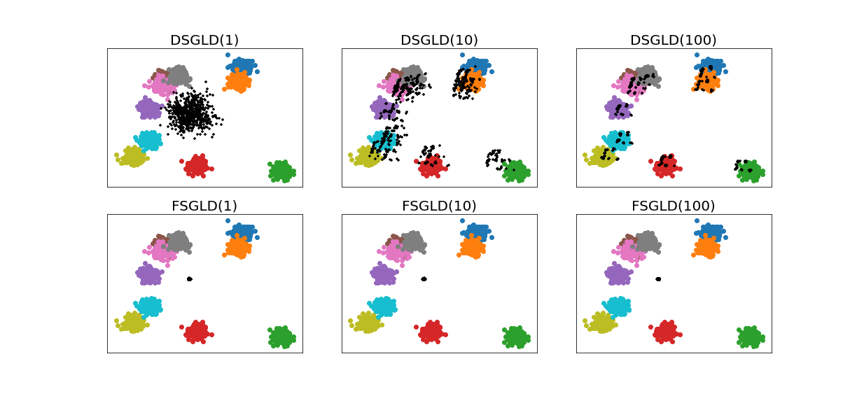
Figure 2: Posterior samples of the global mean (black) in DSGLD and FSGLD, as a function of the number of shard-local updates (shown in parentheses in each title). The colored dots are the data samples, different shards having different color. FSGLD converges to the target posterior in all cases, while DSGLD approaches a mixture of local posteriors as the number of local updates increases. For reference, 3(a) shows samples from the analytical posterior.

In this Section, we demonstrate the performance of our method (FSGLD) for increasingly complex models under the non-IID data regime, which is a defining characteristic of federated settings.

In Subsection 5.1, we show that DSGLD quickly diverges from the true posterior as the frequency of communication decreases, even for very simple models. On the other hand FSGLD easily circumvents this pathology with the help of conducive gradients. In Subsection 5.2, we consider the task of inferring Bayesian metric learning posteriors from highly non-IID data. Finally, in Subsection 5.3, we show how our method can be employed to learn Bayesian neural networks in a distributed fashion, comparing it against DSGLD for both federated IID and non-IID data.

While these models are progressively more complex, we highlight that, using simple multivariate Gaussians as the approximations $q_{1},\ldots,q_{S}$ to each client’s likelihood function, we are still able to obtain good and computationally scalable results for FSGLD. For the first set of experiments, we derive analytic forms for the approximations $q_{s}$, which is only possible due to the simplicity of the target model. For the remaining experiments, we employ SGLD independently for $s=1,\ldots,S$ and use the samples obtained to compute the mean vector and covariance matrix that parameterize $q_{s}$. We implemented all experiments using PyTorch . We also show additional experiments in the supplementary material.

It is important to highlight that, due to our choice of exponential family surrogates, the cost of evaluating conducive gradients in the following experiments compares to an additional prior evaluation.

5.1 non-IID data and delayed communication

An ideal sampling scheme would, in theory, update the chain once at a device and immediately pass it over to another device in the next iteration. However, such a short communication cycle would result in a large overhead and is unrealistic in federated settings. To ameliorate the problem, Ahn et al. [2014] proposed making a number of chain updates before moving to another device. However, the authors reported that as the number of iterations within each client and shard increases, the algorithm tends to lose sample efficiency and effectively sample from a mixture of local posteriors, $\frac{1}{S}\sum_{s=1}^{S}p(\theta|\mathbf{x}_{s})$, instead of the true posterior. With heterogeneous data shards, the effect is particularly noticeable. In this experiment, we illustrate the pathology and show how FSGLD overcomes it.

Model: We consider inference for the mean vector $\mu$ of normally distributed data under the simple model

$$p(\mu|\mathbf{x})\propto\mathcal{N}(\mu|\mathbf{0},I)\prod_{s=1}^{S}\mathcal{N}(\mathbf{x}_{s}|\mu,I).$$ (9)

Setting: We generate $S=10$ disjoint subsets $\mathbf{x}_{1},\ldots,\mathbf{x}_{S}$ of size $200$, each respectively from $\mathcal{N}(\mu_{1},I)$ with $\mu_{1}$ uniformly sampled from the $[-6,6]\times[-6,6]$ square (the colored dots in Fig 2). We then perform inference on the overall mean $\mu$ using the model (9). We sample the same number of posterior samples using both DSGLD and FSGLD with fixed step-size $h=10^{-4}$, mini-batch size $m=10$ and $f_{1}=\cdots=f_{S}=1/S$. The first $20000$ samples were discarded, and the remaining ones were thinned by 100.

Choice of $q_{s}$’s: We use analytic Gaussian surrogates $q_{s}(\theta)=\mathcal{N}(\theta|\overline{\mathbf{x}}_{s},N^{-1}I)$, for each $s=1\ldots S$. Note that $q_{s}$ here is exactly likelihood function induced by the shard $\mathbf{x}_{s}$.

Results: Figure 2 shows the posterior samples as a function of the number of local updates the method takes before passing the chain to the next device. For comparison, Figure 3(a) shows samples from the analytical posterior. As we can see from the results, the proposed method (FSGLD) converges adequately to the true posterior while DSGLD diverges towards a mixture of local approximations. This discrepancy becomes more prominent as we further increase the number of local updates, therefore delaying communication. Figure 3(b) compares the convergence in terms of the number of posterior samples. While DSGLD with a hundred local updates converges as fast as FSGLD, it plateaus at a higher MSE. Note that in contrast with DSGLD, FSGLD is insensitive to the number of local updates in the current experiment.

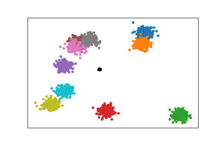
(a)

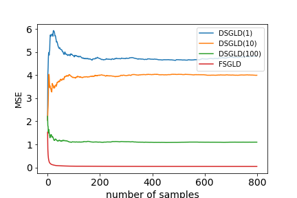
(b)

Figure 3: (a) Samples from the analytical posterior, for comparison with Figure 2. (b) Quantitative comparison of MSE $|\bar{\mu}-\hat{\mu}|^{2}$ in estimating the global mean, as a function of the number of posterior samples, showing FSGLD clearly outperforms DSGLD. Numbers in parentheses indicate number of successive local shard updates; for FSGLD the curves are almost identical, independently of the number, and only one is shown. Only FSGLD converges to $\bar{\mu}$.

Quantifying $\epsilon_{s}^{2}$’s.

Theorem 2 states that the upper-bound on the MSE of FSGLD deteriorates as $\epsilon_{1}^{2},\ldots,\epsilon_{S}^{2}$ increase. While computing $\epsilon_{s}^{2}$’s is intractable for most models, we can approximate it in this simple case using a grid. The same can be done for $\gamma_{s}^{2}$’s, which govern the DSGLD bound in a similar manner. Figure 4 shows that $\epsilon_{s}^{2}\ll\gamma_{s}^{2}$ for all shards $s$. This phenomenon also corroborates with the results in 3(b), which show that the MSE of FSLGD converges to much smaller values than DSGLD.

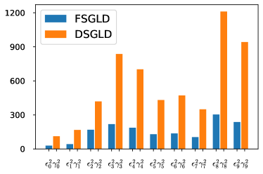
Figure 4: The constants $\epsilon_{s}^{2}$’ s, which govern our method (FSGLD), are much smaller than $\gamma_{s}^{2}$’ ’s from DSGLD, resulting in tighter bounds. The bar plot shows grid-based approximations these for these values in the mean estimation model, in Equation 9.

5.2 Metric learning

Given sets of similar $\mathcal{S}$ and dissimilar $\mathcal{D}$ pairs of vectors from $\mathcal{X}=\{x_{n}\}_{n=1}^{N}\in\mathbb{R}^{D}$, metric learning concerns the task of learning a distance metric matrix $A\in\mathbb{R}^{D\times D}$ such that the Mahalanobis distance

$$\|x_{i}-x_{j}\|_{A}=\sqrt{(x_{i}-x_{j})^{\intercal}A(x_{i}-x_{j})}$$

is low if $(x_{i},x_{j})\in\mathcal{S}$ and high if $(x_{i},x_{j})\in\mathcal{D}$.

Model: We consider inference on the Bayesian metric learning model proposed by Yang et al. [2007], in which it is assumed that $A$ can be expressed as $\sum_{k}\gamma_{k}\mathbf{v}_{k}\mathbf{v}_{k}^{\intercal}$ where $\mathbf{v}_{1},\ldots,\mathbf{v}_{K}$ are the top $K$ eigenvectors of $X=[x_{1}^{\intercal},\ldots,x_{N}^{\intercal}]$. The likelihood function for each pair $(x_{i},x_{j})$ from $\mathcal{S}$ or $\mathcal{D}$ is given by

$$\begin{split}y_{ij}|(x_{i},x_{j}),A,\mu\sim&\text{Ber}\left(\frac{1}{1+\exp\left(y_{ij}\left(\|x_{i}-x_{j}\|_{A}^{2}-\mu\right)\right)}\right)\end{split}$$

where $y_{ij}$ equals one if $(x_{i},x_{j})\in\mathcal{S}$ and equals zero, if $(x_{i},x_{j})\in\mathcal{D}$. While having $\bm{\gamma}=[\gamma_{1},\ldots,\gamma_{K}]\succ 0$ is enough to guarantee that $A$ is positive definite and defines distance metric, this requirement is relaxed and a diagonal Gaussian prior is put both on $\bm{\gamma}$ and $\mu$. For a more thorough treatment, we refer the reader to the original work by Yang et al. [2016].

Setting: We have devised a dataset for metric learning based on the Spoken Letter Recognition (isolet) data, which encompasses 7797 examples split among 26 classes. We have created $|\mathcal{S}|=5000$ and $|\mathcal{D}|=5000$ pairs of similar and dissimilar vectors, respectively, using the labels of the isolet examples, i.e., samples are considered similar if they belong to the same class and dissimilar otherwise. To obtain a federated non-IID dataset, we split these pairs into $S=10$ data shards of identical size, in a manner that there is no overlap in the classes used to create the sets of pairs $\mathcal{S}_{s}$ and $\mathcal{D}_{s}$ in each shard $s=1\ldots S$. Additionally, we created another thousand pairs of equally split similar and dissimilar examples that we hold out for the test.

Choice of $q_{s}$’s: We set $f_{1}=\ldots=f_{S}=\frac{1}{S}$ and run both DSGLD and FSGLD with constant step size $10^{-3}$ and mini-batch size $m=256$. We use simple Gaussian approximations for $q_{1},\ldots,q_{S}$, with mean and covariance parameters computed numerically using three thousand samples from

$$\prod_{(x_{i},x_{j})\in\mathcal{S}_{s}\cup\mathcal{D}_{s}}\text{Ber}\left(y_{i}\big{|}\frac{1}{1+\exp\left(y_{ij}\left(\|x_{i}-x_{j}\|_{A}^{2}-\mu\right)\right)}\right),$$

obtained running SGLD independently for each client. It is worth highlight that these approximations are only computed once at the beginning of training, and then communicated to the server. Appendix F.2 shows additional results using Laplace approximations.

Results: Figure 5 shows results in terms of average log-likelihood as a function of the number of samples. The results show that $i$) FSGLD achieves better performance than DSGLD both in learning and on test data; and $ii$) FSGLD is more communication-efficient than DSGLD, i.e., it converges faster. Furthermore, FSGLD exhibits overall lower standard deviation.

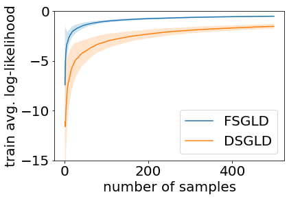
(a)

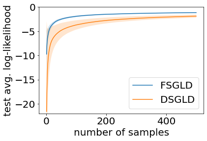
(b)

Figure 5: Metric learning. Average log-likelihood values as a function of the number of samples for both DSGLD and FSGLD, measured on (a) learning data and (b) on a held-out set of test samples.The curves show the mean and standard deviation (error bars) for ten repetitions of the experiment, with different random seeds. FSGLD converges faster and to better predictions than DSGLD, both for training data and for test data.

5.3 Bayesian neural networks

We now gauge the performance of the proposed FSGLD for posterior inference on a deep Multi-Layer Perceptron (MLP) both for federated IID and for federated non-IID data.

Model: We consider an MLP with three hidden layers. The first two hidden layers consist of $18$ nodes each, and the last one of $8$. We equip all hidden nodes with the rectified linear unit (ReLU) activation function, and we apply the Softmax function to the output of the network. Since we employ this network for a classification task, we use the cross-entropy loss function.

Setting: For this experiment, we create a series of $S=30$ label-imbalanced data shards based on the SUSY dataset. For the IID case, we draw the proportions $\pi_{1},\ldots\pi_{S}$ of positive samples in each shard $s=1,\ldots,S$ from a symmetric Beta distribution with parameters $a=b=100$. In this case, each data shard is approximately balanced. For the non-IID case, we sample the proportions from a Beta with both parameters equal to $0.5$ instead. When $a=b=0.5$, half of the shards tend to have mostly positive and the other half tends to have mostly negative labels, enforcing diversity between shards.

All the shards mentioned above comprise $9\times 10^{4}$ samples, and we hold out an additional balanced shard for evaluation. We ran FSGLD and DSGLD, with even shard selection probabilities, for $5\times 10^{3}$ rounds of communication, between which $40$ shard-local updates take place. For both methods, we adopt fixed step-size $h=10^{-4}$ and use mini-batches of size $m=50$. The first $2\times 10^{4}$ samples were discarded for each method, and the remaining ones were thinned by two.

Choice of $q_{s}$’s: Similarly to the previous experiment, we computed the conducive terms by drawing three thousand samples independently from densities proportional to the local likelihoods and imposing diagonal-multivariate normal approximations based on these samples.

Results: Table 1 shows results in terms of average log-likelihood, evaluated on test and train data. For the non-IID case, FSGLD significantly outperforms DSGLD on the test set. It is worth noting the low average log-likelihood achieved by DSGLD during training is a clear sign that it converged to models that do not generalize well. For the IID case, both methods perform similarly. In both cases, FSGLD shows a steep decrease in variance.

Table 1: MLPs. Average log-likelihood for MLPs learned with DSGLD and FSGLD. For the non-IID case, FSGLD clearly learns better models. For the IID case, both methods show similar performance. Results reflect the outcome of ten repetitions (mean $\pm$ standard deviation). For all cases, FSGLD results in smaller standard deviation.

		Homogenous	Heterogenous
		(IID)	(non-IID)
DSGLD	train	-0.69$\pm$0.001	-0.44$\pm$0.062
	test	-0.70$\pm$0.001	-1.11$\pm$0.312
FSGLD	train	-0.69$\pm$0.00022	-0.67$\pm$0.03
	test	-0.69$\pm$0.00022	-0.67$\pm$0.03

6 Related work

Variance reduction for stochastic optimization. Variance reduction has been previously explored to improve the convergence of stochastic gradient descent [e.g. Johnson and Zhang, 2013, Defazio et al., 2014b, a]. While federated optimization has gained increasing attention [Konecný et al., 2016], variance reduction for distributed stochastic gradient descent has received only limited attention [De and Goldstein, 2016, Li et al., 2020] so far.

Variance reduction for serial SG-MCMC. Previous works by Dubey et al. [2016], Baker et al. [2019] have proposed strategies to alleviate the effect of high variance in SGLD, for serial settings. Dubey et al. [2016] proposed two algorithms, SAGA-LD and SVRG-LD, both of which are based on using previously evaluated gradients to approximate gradients for data points not visited in a given iteration. The first algorithm, SAGA-LD, requires a record of individual gradients for each data point to be maintained. In the second one, SVRG-LD, the gradient on the entire data set needs to be periodically evaluated. The recently proposed SGLD-CV Baker et al. [2019] uses posterior mode estimates to build control variates, which are added to the gradient estimates to speed up convergence. Like SGLD-CV, our algorithm can be seen as a control variate method [Ripley, 1987], but designed for distributed (federated) settings.

Distributed/parallel SG-MCMC. In the context of distributed SGLD, Li et al. [2019] did some work proposing different communication protocols and analyzing their impact on convergence. Differently from our work, they do not focus on the impact of heterogeneity among data shards, which is key to federated settings.

7 Conclusion

In this work, we propose conducive gradients, a simple yet effective mechanism that leverages approximations of each device’s likelihood contribution and improves the convergence of SGLD for federated data.

We demonstrate i) that our method converges in scenarios where DSGLD fails, and ii) that it significantly outperforms DSGLD in federated non-IID scenarios. Additionally, our method can be seen as a variance reduction strategy for DSGLD. To the best of our knowledge, this is the first treatment of SG-MCMC for federated settings.

We also analyze the convergence of DSGLD to understand the influence of both data heterogeneity and device availability. We also show convergence bounds for FSGLD and discuss how it supports our choice of local likelihood surrogates.

Furthermore, given suitable surrogates $q_{1},\ldots,q_{S}$, such as exponential family approximations, FSGLD can be simultaneously made efficient both in terms of memory and computation, imposing no significant overhead compared to DSGLD. Nonetheless, we believe that, for very complex models, it could be useful to update the conducive terms as the chains navigate the posterior landscape. We also leave open the possibility of employing more expressive or computationally cheaper surrogates $\{q_{s}\}_{s=1}^{S}$, such as non-parametric methods or variational approximations.