Spectroscopic Orbits of Eleven Nearby, Mid-to-Late M Dwarf Binaries

Abstract

We present the spectroscopic orbits of eleven nearby, mid-to-late M dwarf binary systems in a variety of configurations: two single-lined binaries (SB1s), seven double-lined binaries (SB2s), one double-lined triple (ST2), and one triple-lined triple (ST3). Eight of these orbits are the first published for these systems, while five are newly identified multiples. We obtained multi-epoch, high-resolution spectra with the TRES instrument on the 1.5m Tillinghast Reflector at the Fred Lawrence Whipple Observatory located on Mt. Hopkins in AZ. Using the TiO molecular bands at $7065--7165$ Å, we calculated radial velocities for these systems, from which we derived their orbits. We find LHS 1817 to have in a 7-hour period a companion that is likely a white dwarf, due to the ellipsoidal modulation we see in our MEarth-North light curve data. We find G 123-45 and LTT 11586 to host companions with minimum masses of 41 $M_{Jup}$ and 44 $M_{Jup}$ with orbital periods of 35 and 15 days, respectively. We find 2MA 0930$+$0227 to have a rapidly rotating stellar companion in a 917-day orbital period. GJ 268, GJ 1029, LP 734-34, GJ 1182, G 258-17, and LTT 7077 are SB2s with stellar companions with orbital periods of 10, 96, 34, 154, 5, and 84 days; LP 655-43 is an ST3 with one companion in an 18-day orbital period and an outer component in a longer undetermined period. In addition, we present radial velocities for both components of L 870-44AB and for the outer components of LTT 11586 and LP 655-43.

1 Introduction

Stellar multiplicity is known to be a decreasing function of primary mass, where low-mass main sequence stars have stellar companions less frequently than more massive stars. The multiplicity rate (MR) is the percentage of all systems with a particular primary mass that are multiple, regardless of whether the system is double, triple, or higher order. Solar-type stars have an MR of roughly 46% (Raghavan et al., 2010),  while the MR for M dwarfs appears to be converging on values around 27% (Duchêne & Kraus, 2013; Ward-Duong et al., 2015; Winters et al., 2019). Suggestions for this observed mass dependence include the dynamical stripping of companions from their more massive primaries on gigayear timescales and/or a metallicity dependence in the binary formation environment (Duchêne & Kraus, 2013); this topic remains an area of active research.

However, the closest M dwarfs have not been surveyed comprehensively with the high-resolution techniques necessary to detect companions at the smallest separations, so our understanding of the distribution of the orbital parameters (periods, mass ratios, separations, eccentricities) of M dwarf binaries remains incomplete. Orbital measurements provide important constraints to binary star formation and evolutionary models at the low-mass end of the stellar main sequence. For example, binary star formation models can be probed by fitting the shape of the orbital period distribution. Differentiating between a log-normal or a power law fit would illuminate whether star formation has a preferred spatial scale or follows a scale-free process, respectively, in the formation of binaries (Duchêne & Kraus, 2013). Stars with large space motions are typically old, while slow-moving stars are typically young. Evolutionary models can be constrained by exploring multiplicity as a function of space motion by using the gamma velocity of the system, a valuable result of orbit measurements. Winters et al. (2019) found a decreasing trend of stellar multiplicity with increasing tangential velocity for M dwarfs. The calculation of three dimensional $UVW$ space motions from the combination of gamma velocities with the proper motions of binary systems permits a robust investigation of this trend. Further, the resulting minimum masses from orbit measurements, when combined with inclinations from astrometric orbits (where the components are unresolved), yield dynamical masses for these low-mass objects. Yet, within 25 pc, only a few dozen M dwarf systems have measured spectroscopic orbits, mostly with early-type M dwarf primaries; within 15 pc, only nine mid-to-late M-dwarf (0.1 – 0.3 M_⊙) multiples have published spectroscopic orbits (Lacy, 1977; Delfosse et al., 1999a; Ségransan et al., 2000; Nidever et al., 2002; Baroch et al., 2018).

Part of the reason for the dearth of spectroscopic orbits with M dwarf primaries is that their intrinsically low luminosities have made them historically challenging targets to study. This faintness is compounded by the multi-epoch observations required to detect radial velocity variations. Thus, early spectroscopic work on M dwarfs focused on bright, typically early-type M dwarf targets (Duquennoy & Mayor, 1988; Marcy & Benitz, 1989; Tokovinin, 1992; Mazeh et al., 2003).

However, the M dwarf spectral sequence spans a magnitude difference of 11.2 in $M_{V}$ (8.8 – 20.0 mag) and a factor of 8 in mass (0.08 – 0.64 M/M_⊙). Thus, the orbital parameters of binaries with more massive, early-type M dwarf primaries are not necessarily predictive of those with mid-to-late M dwarf primaries. More work needs to be done to characterize binaries with later-type primaries. Fortunately, modern spectrographs now allow us to push toward fainter targets and larger samples, as illustrated by the work presented in Delfosse et al. (1999a, b); Nidever et al. (2002); Shkolnik et al. (2010); Davison et al. (2014); Baroch et al. (2018).

We are conducting an all-sky, volume-complete, multi-epoch, high-resolution spectroscopic survey of 412 mid-to-late M dwarfs (0.1 – 0.3 M_⊙) within 15 pc for companions. For targets north of $\delta$ $=-$15°, we are using the Tillinghast Reflector Echelle Spectrograph (TRES) on the 1.5m telescope at the Fred Lawrence Whipple Observatory (FLWO) on Mt. Hopkins, AZ. For targets south of $\delta=-$15°, we are using the CTIO HIgh ResolutiON (CHIRON) spectrograph at the Cerro Tololo Inter-American Observatory / Small and Moderate Aperture Research Telescope System (CTIO / SMARTS) 1.5m telescope. During the TRES portion of our survey, we have discovered six new spectroscopic multiple systems to-date. One system, LHS 1610Ab, was previously presented in Winters et al. (2018); we do not include it here. Here we present the spectroscopic orbits of eleven multiples containing 24 components; in addition, we present the velocities of L 870-44AB, a very long-period binary that shows doubled lines, for which we have not measured an orbit. Future papers from this project will present the full sample of mid-to-late M dwarfs within 15 pc, along with their radial and rotational velocities, H_α equivalent widths, $UVW$ space motions, and a thorough analysis of the multiplicity of this volume-complete sample.

2 Sample Selection

All of the systems presented here were thought to have primary masses 0.1 – 0.3 M/M_⊙ and to lie within 15 pc (corresponding to a parallax $\pi>66.67$ mas), either via a trigonometric parallax or a photometric distance estimate. Results from the Gaia second data release (DR2) (Gaia Collaboration et al., 2018; Lindegren et al., 2018) provided new or revised parallaxes for all of them. As expected, systems that were discovered to be nearly equal-luminosity binaries that previously had only photometric distance estimates now lie beyond 15 pc via their trigonometric parallax, as light from the unresolved secondary made the system overluminous and resulted in an underestimated photometric distance. This was the case for three systems presented here: L 870-44, LP 655-43, LP 734-34. In addition, G 258-17 had a parallax that placed it beyond 25 pc, of which we became aware only after we discovered it was a new SB2 and began measuring its orbit. Table 2 lists the astrometric data from the Gaia DR2 for the systems presented here, where the coordinates were adjusted for proper motion from the epoch of the 2MASS observations to epoch 2000.0 using the DR2 proper motions (Gaia Collaboration et al., 2018) and the 2MASS right ascenscion, declination, and Julian date (Skrutskie et al., 2006) for each object. We additionally list the best-known distance at the time before the availability of the DR2, which led to the inclusion of each system in our sample, as well as the DR2 parallax. The initial parallaxes listed for GJ 1029AB and GJ 268AB represent weighted mean parallaxes.

Masses were estimated using the M_K mass-luminosity relation (MLR) by Benedict et al. (2016) under the assumption that the objects were single stars. Three exceptions to this are GJ 268AB, LTT 11586AcB, and LTT 7077AB, which were already reported in the literature to be spectroscopic binaries. We elected to measure the orbit of GJ 268AB as a check for our method (see §4.3.1) with the knowledge that the primary’s mass was within the range of our sample (i.e., from the orbit presented in Delfosse et al., 1999a). We chose to measure the spectroscopic orbits of LTT 11586AcB and LTT 7077AB, systems with no published orbits, under the assumption that they were nearly-equal-magnitude binaries and that the primary masses from the measured orbits would then fall within the range of targeted stellar masses in our sample. Table 2 provides the optical and infrared photometric data for the sample, where available. All photometry measured by Weis (i.e., Weis, 1991, 1996, 1999) has been converted to the Johnson-Kron-Cousins (JKC) system using the relation in Bessell & Weis (1987). In addition, we list each object’s initial mass estimate (from the initial parallaxes in Table 2, in combination with the $K-$band magnitude in Table 2), and the types of spectroscopic multiple for each system. We note that the initial mass estimates are incorrect, as they include light from the companion star and/or their initial distances were erroneous. We list them here to illustrate how these objects came to be intially included in our sample. More accurate masses can be derived from the results of our orbit determinations under the assumption that there are no more unresolved stars in the system. We also indicate whether the multiple system is a new discovery (‘New Mult?’) and whether the orbit presented here is the first orbit measured for the system (‘First Orbit?’). We note that, aside from GJ 1029AB, L 870-44AB, GJ 268AB, and GJ 1182AB, these are the first spectroscopic orbits measured for these systems. In the cases of GJ 1029AB and GJ 1182AB, we only became aware of their previously published orbits by Baroch et al. (2018) after we had completed our orbit determinations for those systems. L 870-44AB has no published orbit, and we do not report one here.

Table 1: Astrometric Data for Multiple Systems

Name	2MASS ID	R.A.	decl.	$\mu_{\rm RA}$	$\mu_{\rm decl}$	$\pi_{init}$	Ref	$\pi_{DR2}$
		(hh:mm:ss)	(dd:mm:ss)	(mas yr-1)	(mas yr-1)	(mas)		(mas)
GJ 1029AB	01053732$+$2829339	01:05:37.6	$+$28:29:34	1914.461	-188.452	83.70$\pm$2.19	1,3	79.84$\pm$0.34
L 870-44AB	01463681$-$0838578	01:46:36.8	$-$08:38:58	412.840	-182.424	68.49$\pm$10.6*	5	39.10$\pm$1.05
LP 655-43ABC	04380252$-$0556132	04:38:02.5	$-$05:56:13	-63.909	-180.631	68.03$\pm$10.9*	5	27.19$\pm$0.30
LTT 11586AcB	05074924$+$1758584	05:07:49.2	$+$17:58:58	32.012	-261.584	101.90$\pm$6.00	2	86.10$\pm$0.31
LHS 1817Ab	06052936$+$6049231	06:05:29.4	$+$60:49:23	289.645	-788.403	71.30$\pm$2.20	1	61.13$\pm$0.15
GJ 268AB	07100180$+$3831457	07:10:01.8	$+$38:31:46	-439.670	-944.785	163.41$\pm$1.78	3,4	164.64$\pm$0.13
2MA 0930+0227AB	09305084$+$0227202	09:30:50.8	$+$02:27:20	-33.530	80.977	71.30$\pm$7.20	2	44.50$\pm$0.37
LP 734-34AB	12102834$-$1310234	12:10:28.4	$-$13:10:24	246.653	-343.832	71.94$\pm$11.7*	5	45.45$\pm$0.08
G 123-45Ab	12362870$+$3512007	12:36:28.7	$+$35:12:01	-360.030	-117.185	88.20$\pm$1.70	1	84.01$\pm$0.21
GJ 1182AB	14153253$+$0439312	14:15:32.6	$+$04:39:31	-744.931	-766.435	71.70$\pm$3.40	3	71.11$\pm$0.39
G 258-17AB	17411611$+$7226320	17:41:16.1	$+$72:26:32	-124.133	301.274	77.60$\pm$5.00	1	33.53$\pm$0.05
LTT 7077AB	17462934$-$0842362	17:46:29.4	$-$08:42:37	-44.202	-428.041	77.18$\pm$1.71	6	76.59$\pm$0.08

References. — (1) Dittmann et al. (2014); (2) Finch et al. (2018); (3) van Altena et al. (1995); (4) van Leeuwen (2007); (5) Winters et al. (2015); (6) Winters et al. (2017).

Note. — Proper motions $\mu_{\rm RA}$, $\mu_{\rm decl}$ and parallaxes $\pi_{DR2}$ are from the Gaia DR2 (Gaia Collaboration et al., 2018; Lindegren et al., 2018). An * next to the $\pi_{init}$ indicates that the listed ‘parallax’ is a photometric distance estimate.

Table 2: Photometric and Spectroscopic Data for Multiple Systems

Name	$G$	$V_{J}$	$R_{KC}$	$I_{KC}$	Ref	$J$	$H$	$K_{s}$	massinit	Type	New	First
	(mag)	(mag)	(mag)	(mag)		(mag)	(mag)	(mag)	(M/M⊙)		Mult?	Orbit?
GJ 1029AB	12.97	14.79J	13.29J	11.37J	4	9.486J	8.881J	8.550J	0.16$\pm$0.02	SB2	no	no
L 870-44AB	11.73	12.99J	11.82J	10.30J	5	8.832J	8.237J	7.994J	0.28$\pm$0.06	SB2	no	N/A
LP 655-43ABC	12.91	14.44J	13.14J	11.41J	1	9.730J	9.136J	8.818J	0.18$\pm$0.04	ST3	yes	yes
LTT 11586AcB	10.69	11.80J	10.69J	9.32J	3	8.023J	7.446J	7.178J	0.27$\pm$0.03	ST2	no	yes
LHS 1817Ab	12.30	13.69	12.50	10.84	4	9.096	8.464	8.176	0.24$\pm$0.02	SB1	no	yes
GJ 268AB	9.93	11.42J	10.16J	8.45J	4	6.731J	6.152J	5.846J	0.32$\pm$0.02	SB2	no	no
2MA 0930+0227AB	12.40	$\cdots$	$\cdots$	$\cdots$	$\cdots$	9.415J	8.856J	8.578J	0.19$\pm$0.03	SB2	yes	yes
LP 734-34AB	12.32	13.83J	12.52J	10.85J	6	9.292J	8.684J	8.412J	0.21$\pm$0.04	SB2	yes	yes
G 123-45Ab	12.26	13.80	12.45	10.77	2	9.113	8.542	8.261	0.18$\pm$0.02	SB1	yes	yes
GJ 1182AB	12.67	14.30J	12.95J	11.09J	4	9.433J	8.936J	8.618J	0.18$\pm$0.02	SB2	no	no
G 258-17AB	13.34	$\cdots$	$\cdots$	$\cdots$	$\cdots$	10.275J	9.706J	9.442J	0.12$\pm$0.02	SB2	yes	yes
LTT 7077AB	11.27	12.72J	11.44J	9.78J	6	8.198J	7.693J	7.353J	0.35$\pm$0.02	SB2	no	yes

Note. — ‘J’ indicates that the photometry is joint and therefore includes light from one or more companions. ‘SB1’: single-lined binary, ‘SB2’: double-lined binary, ‘ST2’: double-lined triple, ‘ST3’: triple-lined triple. Gaia $G$ photometry from Gaia Collaboration et al. (2018); 2MASS $JHK$ photometry from Skrutskie et al. (2006).

References. — (1) Reid et al. (2002); (2) RECONS, in prep (Silverstein et al.); (3) Weis (1991); (4) Weis (1996); (5) Weis (1999); (6) Winters et al. (2015).

3 Data Acquisition

We observed each object between UT 2016 October 14 and 2020 January 08 using TRES on the FLWO 1.5m Tillinghast Reflector. TRES is a high-throughput, cross-dispersed, fiber-fed, echelle spectrograph. We used the medium fiber ($2\farcs 3$ diameter) for a resolving power of $R\simeq 44\,000$. The spectral resolution of the instrumental profile is 6.7 km s^-1 at the center of all echelle orders. For calibration purposes, we acquired a thorium-argon hollow-cathode lamp spectrum through the science fiber both before and after every science spectrum. Exposure times ranged from $120$s to $3$ $\times$ $1200$s in good conditions, achieving a signal-to-noise ratio of 3-25 per pixel at $7150\ {\rm\AA}$ (the pixel scale at this wavelength is $0.059\ {\rm\AA~{}pix^{-1}}$). These exposure times were increased where necessary in poor conditions. The spectra were extracted and processed using the standard TRES pipeline (Buchhave et al., 2010).

We describe here the temperature and pressure control of TRES. TRES has two stages of temperature control. The spectrograph is housed inside a custom enclosure with fine temperature control, which in turn is located in the coude room, which has coarse temperature control. The temperature is monitored at more than a dozen key locations and the values are reported in the header of each observation. Over several hours the variation is typically less than about 0.1 K at the spectrograph bench and echelle grating, with slow drifts from season to season of about 1 K. There is no pressure control, so all science observations are sandwiched between wavelength calibrations using a thorium-argon hollow-cathode lamp. Drifts in the zero point of the velocity system are monitored using nightly observations of well-established radial-velocity standard stars, typically 3 or 4 per night. These procedures are able to correct for drifts in the zero point of the velocity system to better than 10 m s^-1 from month to month, and better than about 30 m s^-1 since 2013. Orbital solutions for bright slowly-rotating stars typically have rms velocity residuals of 20 m s^-1, which is a good indicator of the single-measurement precision when photon noise does not set the limit.

4 Spectroscopic Analysis & Radial Velocity Measurements

We use a template spectrum of Barnard’s Star, observed on UT 2018 July 19, to perform cross-correlations based on the methods described in Kurtz & Mink (1998). Barnard’s Star is a slowly rotating (130.4 days, Benedict et al., 1998) M4.0 dwarf (Kirkpatrick et al., 1991) for which we adopt a Barycentric radial velocity of $-110.3\pm 0.5\ {\rm km\ s^{-1}}$, derived from presently unpublished CfA Digital Speedometer (Latham et al., 2002) measurements taken over 17 years. We see negligible rotational broadening in our Barnard’s Star template, in agreement with the $v\sin i$ of 0.07 km s^-1 expected from the 130.4-day photometric rotation period noted above. This is also consistent with the $v\sin i$ upper limit of $2~{}{\rm km\ s^{-1}}$ reported by Reiners et al. (2018). We use the wavelength range 7065 to 7165Å (echelle aperture 41) for the correlations, a region that is dominated by TiO bandhead features in mid-to-late M dwarfs, which provide many lines for the radial velocity (RV) measurements (Irwin et al., 2011). Part of the red end of the aperture is not included, as it is contaminated by telluric absorption features.

For the double- and triple-lined systems, we use a least-squares deconvolution (LSD; Donati et al., 1997) method to identify double- or multi-lined systems and to estimate the initial light ratios between the components. We then used these as starting points for todcor and tricor (Zucker & Mazeh, 1994; Zucker et al., 1995), which calculate the RV of each component in the double- and triple-lined systems, respectively. As with the single-lined systems, we used our observed Barnard’s Star spectrum as the template for all components. In each case, we search for the light ratio with the maximum correlation peak in echelle aperture 41, which we then uniformly apply to all observations of each system to measure the velocities. This assumes that there are no significant photometric or spectroscopic variations in any of the stars in the system.

Aside from LHS 1817A, LTT 11586B, and 2MA 0930AB, none of the primary stars or components show any appreciable rotational broadening at the resolution of the TRES spectra, so there was no need to broaden the template spectrum in order to obtain a good match. Therefore, we assumed a $v\sin i$ of zero for all systems presented here, except for the three noted above. Because the light ratio is dependent upon the $v\sin i$ in the double-lined systems, we chose ever finer grids of $v\sin i$, for which we determined the light ratio that produced the maximum correlation peak via todcor. We then fit preliminary orbits based on each set of resulting RVs. We chose the $v\sin i$ and light ratio that resulted in an orbital fit to the RVs with the smallest residuals. For the three systems noted above, the projected rotational velocities used to calculate the RVs are indicated in the the notes on those systems.

We use the Wilson method (Wilson, 1941) to estimate the initial mass ratio q $=$ m₂/m₁ and gamma velocity of the system as inputs for the orbital fit. In short, we plot the velocities of the primary component as a function of the velocities of the secondary component. The negative slope of a linear fit to the velocities provides the mass ratio, and the y-intercept divided by ($1+q$) provides the gamma velocity.

Variations in the instrumental line profile on the order of 0.1 km s^-1 result in systematic errors on components’ velocities that render them unreliable when their velocity difference is less than roughly 2 km s^-1. We thus adopt 3.4 km s^-1, i.e., half the spectral resolution of TRES, as a conservative upper limit to the components’ velocity difference and omit data where it is less than this.

For systems that had MEarth data, we searched for evidence of eclipses, which we are able to rule out for LHS 1817 and G 123-45.

4.1 Orbit determination

To determine orbital parameters, we used the same method as previously reported in Irwin et al. (2011); Winters et al. (2018). We fit a standard eccentric Keplerian orbit to the radial velocities of the appropriate components in each system using the emcee package (Foreman-Mackey et al., 2013) to obtain samples from the posterior probability density function of the parameters using Markov Chain Monte Carlo (MCMC).

Estimation of velocity uncertainties from cross-correlation analysis is a notoriously difficult problem, particularly in the case of multiple lined systems, so instead, and for consistency across all the orbital solutions regardless of the number of spectroscopic components, we take a simpler approach and derive the appropriate velocity uncertainties $\sigma$ during model fitting. Separate uncertainties were allowed for each system component because these can sometimes differ substantially, for example in SB2 systems with light ratios very far from unity or with differing amounts of rotational broadening.

In order to reduce the influence of lower quality spectra on the results, the data points were weighted using the square of the normalized peak cross correlation ($h_{i}$, as defined by Tonry & Davis (1979)), where the resulting weights are $1/h_{i}^{2}$ for data point $i$. This is equivalent to adopting a velocity uncertainty of $\sigma/h_{i}$ on data point $i$. These resulting values are reported in Table 3, but it is important to note that they are not conventional, independent velocity uncertainties but are rather derived from the orbit model and are dependent on the assumption that the orbit model is the correct description of the data. We note that we do not include the 0.5 km s^-1 uncertainty on Barnard’s Star’s RV when fitting the orbit for each system. This is because the orbit-fitting depends only on the relative velocity in all parameters except the gamma velocity, and including this uncertainty would cause the total uncertainties to be severely overestimated.

In practice, each solution must be validated by comparing the derived value of $\sigma$ to our expectations based on simulated data or experience from analysis of similar data sets. The standard test of comparing the $\chi^{2}$ value to the number of degrees of freedom as a metric for goodness of fit is rendered useless by fitting for the uncertainty (such solutions always produce this value of $\chi^{2}$, by construction).

The resulting model has 7 free parameters for single-lined orbits, and 9 for double-lined orbits. Five of these are common to both cases: the epoch of inferior conjunction $T_{0}$, the orbital period $P$, systemic radial velocity $\gamma$, $e\cos\omega$, and $e\sin\omega$, where $e$ is eccentricity and $\omega$ is the argument of periastron. For single-lined orbits the remaining pair of parameters are the velocity semi-amplitude $K$ and velocity uncertainty $\sigma$. We calculate masses for the primary components of the single-lined systems using the $K_{s}$ magnitude in Table 2 and the updated parallax $\pi_{DR2}$ listed in Table 2. For double-lined orbits the remaining four parameters are the mass ratio $q$, the sum of the velocity semi-amplitudes of the two components $K_{1}+K_{2}$, and the separate velocity uncertainties for each component $\sigma_{1}$ and $\sigma_{2}$.

This procedure results in a likelihood for the single-lined orbit model (closely following the derivation in Gregory 2005) of:

$$p(D|M)={\exp\left[-\sum_{i=1}^{N}{h_{i}^{2}(v_{i}-m(t_{i}))^{2}\over{2\sigma^{2}}}\right]\over{\sqrt{\prod_{i=1}^{N}2\pi\left({\sigma^{2}\over{h_{i}^{2}}}\right)}}}$$ (1)

where $D$ denotes the data and $M$ the model, $v_{i}$ are the individual radial velocities for each data point $i$ (with $N$ data points total), $h_{i}$ are their normalized peak cross-correlation values, and $m(t_{i})$ is the Keplerian model evaluated at data point $i$ (time $t_{i}$). The product of the normalization constants of the Gaussian distributions for the data points appearing in the denominator of Eq. (1) is often omitted but must be included explicitly when fitting for $\sigma$ because it is no longer constant. In practice, we calculate $\log p(D|M)$ when implementing this method to avoid the exponential and product in Eq. (1) but we have given the equation for the likelihood itself for clarity.

For double-lined orbits each observation results in a pair of velocities, and these were treated as two data points using the same likelihood formulation, but substituting the appropriate $\sigma_{1}$ or $\sigma_{2}$ parameters as needed for each component to replace $\sigma$ in Eq. (1) and calculating the model velocity for the respective component in place of $m$.

For the $\sigma$ parameters we adopt modified Jeffreys priors of the form:

$$p(\sigma)\propto{1\over{\sigma+\sigma_{a}}}$$ (2)

where $\sigma>0$ and $\sigma_{a}>0$ is a constant. The value of $\sigma_{a}$ was set to $10\%$ of the estimated velocity uncertainty, following Gregory (2005), Eq. (16) and surrounding discussion.

The choice of $e\sin\omega$ and $e\cos\omega$ as jump parameters was made for mathematical convenience but has the undesirable feature of producing a linearly increasing prior on $e$ if uniform priors are adopted on these two parameters. In order to avoid this we include a factor of $1/e$ in the prior and reject any points with $e\geq 1$ to convert this to a uniform prior on $e\in[0,1)$.

Uniform improper priors were adopted on all other parameters, resulting in an overall prior probability density function proportional to the product of the factors from Eq. (2) and $1/e$ from the previous paragraph. This was then combined with the $\log$ likelihood from above to obtain the $\log$ posterior returned by the objective function to emcee.

The MCMC simulations were initialized using a Levernberg-Marquardt (L-M) fit of the function $m$ for the Keplerian parameters, and the rms of the residuals of the data about this model were used to initialize the $\sigma$ parameters. One hundred walkers, as described by the emcee method, were then populated with initial values derived by perturbing the L-M fit results by Gaussian random deviates with a standard deviation of $3$ times the estimated parameter uncertainties from the L-M to ensure different starting points for each walker and burned in for $1\times 10^{4}$ samples, followed by $5\times 10^{4}$ samples of the posterior probability density function retained for analysis. The samples from all of the walkers were combined assuming independence resulting in a total of $5\times 10^{6}$ samples, which were converted to a central value and uncertainty using the median and $68.3$ percentile of the absolute deviation from the median, respectively.

This paper also includes orbits for two more complicated triple systems. For these solutions we simply extended the model already described above to allow for a variable $\gamma$ velocity, but otherwise ignored the additional component during fitting and MCMC analysis. These additional (outer) components have incomplete orbits and large period ratios so these models simply used linear or quadratic functions for the $\gamma$ velocity.

We describe each system individually here, ordered from single- to triple-lined systems and by RA within each section. The measured RVs for each system, along with their internal uncertainties, are reported in Table 3. We show the orbital fits to the TRES RVs (top) and residuals to the fits (bottom) in Figures 1 – 7, with primaries shown in blue, secondaries in green, and tertiaries in red. Error bars are smaller than the points in the orbital fit plots, in most cases, and are repeated in the residuals plots. The orbital parameters for GJ 268AB are listed in Table 4, and we present the orbital parameters for all other systems in Table 5, ordered by RA. The only exception is L 870-44AB; no orbit has been derived yet for this system because there are not yet enough data for a robust period determination. Finally, we assign component designations with capital letters if we see the spectral lines and lower case letters if we do not see the lines; for example, we use ‘Ab’ for the single-lined binaries and ‘AB’ for the double-lined binaries. For the triple systems, the component indicators are assigned according to the height of the peak of each component in the least squares deconvolution analysis, where the primary component has the largest peak and is assigned the designation ‘A’.

4.2 Single-lined Systems

We describe the two single-lined systems, LHS 1817Ab and G 123-45Ab.

4.2.1 LHS 1817Ab

This system is a single-lined, spectroscopic binary that was suggested by Newton et al. (2016) to be multiple because of an unphysically metal-rich estimate of the star’s metallicity. We obtained 24 observations of LHS 1817A with S/N per spectral resolution element of 5-18. The typical data processing of the spectra of our targets involves median combining the three exposures usually acquired to minimize the effects of radiation events. However, the combined spectra of this target result in exposure times of 900 - 2700s and comprise a significant fraction of the 7.4-hour orbital period (roughly 3 – 10%), resulting in the velocities smearing. Therefore, we analyze the individual spectra from each set of exposures to calculate the velocities. This generally results in lower, but still usable, correlation function peak heights. We use the mean $v\sin i$ of $27.9\pm 1.3$ km s^-1 from all epochs, in agreement with that of $29.7\pm 2.6$ km s^-1 reported by Kesseli et al. (2018), to calculate the velocities. We estimate a mass of $0.290\pm 0.014$ M/M_⊙ for the primary star. We find an orbital period of $0.30992678\pm 0.00000048$ days, an eccentricity of $0.0063\pm 0.0031$, and a minimum mass ratio of $0.9343\pm 0.0035$. Our measured orbital period is in agreement with the photometric rotation period reported by Newton et al. (2016) and indicates that the system has synchronized, as expected due to the short orbital period. We show the orbital fit and velocity residuals in the left panel of Figure 1.

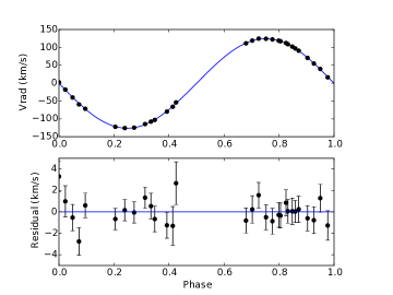
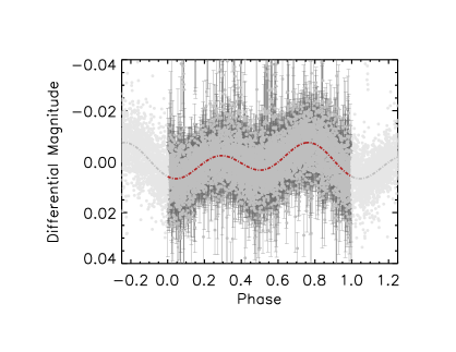
Figure 1: The orbital fit (left) and light curve (right) of LHS 1817A. (Left) The best orbital fit to the velocities is shown in the top panel, while residuals to the fit are indicated in the bottom panel. (Right) The MEarth light curve of LHS 1817A, phase-folded to the orbital (and rotational) period of $0.3099267\pm 0.0000014$ days. The dash-dot red line indicates the fit that includes the ellipsoidal modulation due to the white dwarf. The lighter shaded regions at phases -0.25-0.0 and 1.0-1.25

are duplicated portions of the light curve.

The resulting minimum mass ratio from our orbital fit is near unity, but we do not see a second set of spectral lines from the companion. We therefore expect that the companion is a white dwarf. We have five years of MEarth (Nutzman & Charbonneau, 2008; Irwin et al., 2015) data for this target, taken UT 2011 October 11 – 2016 October 30. The light curve shows two peaks, an indication of ellipsoidal modulation, where a massive companion is tidally distorting the M dwarf into an ellipsoidal shape. This lends strength to our assumption that the companion is a white dwarf. We modeled the ellipsoidal modulation by fitting to the light curve a sine curve plus a second harmonic model. We show the light curve with our fit to the ellipsoidal variation in the right panel of Figure 1, phase-folded to the photometric rotation period.

The amplitude of the ellipsoidal variation depends on inclination as $sin^{2}i$, the ratio of the stellar radius to the semi-major axis $R_{1}/a$, the mass ratio $q$, and limb darkening and gravity darkening (e.g., Shporer 2017). The dependence on inclination is different from that of the semi-amplitude $K$ as a function of the same parameters, so it is possible to infer the inclination by combining these constraints.

In order to do so, we estimate the stellar radius using the mass-luminosity and mass-radius relations, and obtain limb darkening and gravity darkening coefficients from the tabulations of Claret et al. (2012), which require the effective temperature.

We estimate the radius of the M dwarf to be $0.293\pm 0.027$ R_⊙ using the empirical single star mass-radius relation in Boyajian et al. (2012), based on the mass of the star ($0.290\pm 0.014$ M_⊙) calculated using the MLR by Benedict et al. (2016). We note that these relations may not be entirely appropriate for this system, as the M dwarf component likely accreted material from the white dwarf’s progenitor when it evolved off the main sequence. We also find it to be slightly overluminous in the $V-$ and $K-$bands; thus, it falls among the blended photometry binary sequence on an observational Hertzsprung-Russel diagram. We note that the system is X-ray-bright, as previously reported by Shkolnik et al. (2012).

We estimate the effective temperature by combining two relations. Using the Stefan-Boltzmann Law we obtain a value of $3333\pm 150$ K, using the method previously described by Dittmann et al. (2017); Ment et al. (2019). From the ($V-J$), ($J-H$) relation in Mann et al. (2015, 2016), we calculate the effective temperature to be $3207\pm 77$ K. We adopt the unweighted mean of these two values $3270\pm 150$ K.

To infer the inclination, we assume all the signal seen in the second harmonic in the light curve analysis is due to ellipsoidal variation, ignoring the fundamental, which seems to be spot-dominated. While the second harmonic will inevitably be somewhat polluted by spots, the phase being fairly consistent with that of the orbital solution implies that most of the signal is due to the ellipsoidal modulation.

We use an MCMC analysis to obtain the posterior for the inclination, including the mass-luminosity and mass-radius relations, limb darkening and gravity darkening table lookups inside this procedure to allow for the uncertainties. Gaussian priors were adopted for the orbital period, second harmonic semi-amplitude, effective temperature, K magnitude, and parallax derived from the observations as appropriate and the resulting posterior for the inclination analysed as described in §4.1.

The resulting estimate for the orbital inclination is 27.8$\pm$0.96°. This yields a mass for the white dwarf of 1.03$\pm$0.08 M_⊙ and a mass ratio of $3.57\pm 0.14$ for the system.

As a comparison, we can also independently estimate the inclination if we assume that the rotational axis of the M dwarf is aligned with the orbital axis of the binary system. Because we know the photometric rotation period $P_{rot}$ of the M dwarf, as well as its $v\sin i$, we use the relation $P_{rot}*v\sin i=2\pi R\sin i$. We note that the magnitude of the $v\sin i$ may not be due entirely to rotational broadening and may have an additional broadening contribution from other sources for which we have not accounted. From these admittedly imperfect assumptions and adopting ten percent errors for the rotation period, we estimate the inclination of the system to be $36.3\pm 6.3$°. From this inclination, we calculate a mass of $0.64^{+0.25}_{-0.14}$ M_⊙ for the white dwarf, which results in a mass ratio of $2.21^{+0.87}_{-0.50}$ for the system.

Table 3: Radial Velocities for Multiple Systems

BJD	A $v_{\rm rad}$	B $v_{\rm rad}$	C $v_{\rm rad}$	$h$
(days)	(${\rm km\ s^{-1}}$)	(${\rm km\ s^{-1}}$)	(${\rm km\ s^{-1}}$)
GJ 1029AB
2457759.6280	-20.121$\pm$0.123	0.474$\pm$0.964	$\cdots$	0.802994
2457944.9249	-19.027$\pm$0.121	0.165$\pm$0.945	$\cdots$	0.819148
2457993.9720	-6.797$\pm$0.122	-17.107$\pm$0.952	$\cdots$	0.813055
2458002.8908	-7.730$\pm$0.117	-17.120$\pm$0.916	$\cdots$	0.845087
2458027.8068	-13.272$\pm$0.112	-9.713$\pm$0.874	$\cdots$	0.885454
2458034.8799	-16.250$\pm$0.109	-3.582$\pm$0.849	$\cdots$	0.912088
2458042.7260	-19.790$\pm$0.115	0.208$\pm$0.903	$\cdots$	0.857204
2458050.7436	-18.108$\pm$0.111	-1.706$\pm$0.870	$\cdots$	0.889733
2458055.8456	-13.808$\pm$0.109	-9.021$\pm$0.853	$\cdots$	0.907916
2458063.7882	-8.912$\pm$0.114	-14.354$\pm$0.890	$\cdots$	0.869500
2458082.6561	-6.668$\pm$0.113	-18.136$\pm$0.880	$\cdots$	0.879921
2458090.7040	-7.083$\pm$0.120	-18.430$\pm$0.936	$\cdots$	0.826577
2458107.7450	-8.910$\pm$0.116	-13.698$\pm$0.909	$\cdots$	0.851294

Note. — The velocities for the first system in our sample are shown to illustrate the form and content of this table. The full electronic table is available in the online version of the paper.

4.2.2 G 123-45Ab

This is a new single-lined spectroscopic binary. We obtained 19 spectra with S/N per spectral resolution element of 19-39 and see no evidence of broadening due to rotation. We estimate a mass of $0.185\pm 0.014$ M/M_⊙ for the primary star. We find an orbital period of $34.7557\pm 0.0041$ days, an eccentricity of $0.3758\pm 0.0024$, and a minimum mass ratio of $0.20903\pm 0.00049$ for the system. We measure the minimum mass of the companion to be $40.510\pm 0.096$ M_J, significantly below the sub-stellar boundary. We show the resulting orbital fit to the velocities in the left panel of Figure 2.

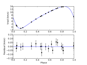
Figure 2: The orbital fits of G 123-45A and GJ 268AB. The best orbital fits to the data for G 123-45A (left) and GJ 268AB (right) are shown in the top panels, while residuals to the fit are indicated in the bottom panels.

4.3 Double-lined Systems

We present the orbit of GJ 268 to illustrate the robustness of our method for double-lined binaries, followed by the results for the remaining systems.

4.3.1 GJ 268AB

The orbit for this well-known, double-lined binary has been previously published (Tomkin & Pettersen, 1986; Delfosse et al., 1999a). We chose to measure the orbit of this system in order to compare the results of our method with previous results. We acquired 10 spectra with S/N per spectral resolution element of 23-34. We see no evidence of rotational broadening and use a light ratio of 0.692 to derive the velocities of the components with todcor. All the velocities were well-separated, with none needing to be discarded. We show the results of our analysis, along with those from Delfosse et al. (1999a) in Table 4. There is excellent agreement between the two orbital solutions, when taking into account the 0.5 km s^-1 RV uncertainty of our Barnard’s Star template. We present the orbital fit for GJ 268AB in the right panel of Figure 2.

Table 4: Comparison of GJ 268AB Orbital Parameters

Parameter	This Work	Delfosse et al. (1999a)
MCMC parameters
$e\cos\omega$	$-0.2721\pm 0.0018$	$\cdots$
$e\sin\omega$	$-0.1736\pm 0.0016$	$\cdots$
$T_{0}$ (BJD)	$2457675.4569\pm 0.0064$	$\cdots$
$P$ (days)	$10.42673\pm 0.00010$	$10.4265\pm 0.00002$
$q$	$0.8505\pm 0.0022$	$0.851\pm 0.001$
$\gamma$ (km s-1)	$42.337\pm 0.039$	$41.83\pm 0.03$
$(K_{1}+K_{2})$ (km s-1)	$75.78\pm 0.13$	$75.67\pm 0.07$
$\sigma_{1}$ (km s-1)	$0.084\pm 0.028$	$\cdots$
$\sigma_{2}$ (km s-1)	$0.131\pm 0.038$	$\cdots$
Derived parameters
$e$	$0.3227\pm 0.0018$	$0.321\pm 0.001$
$\omega$ (deg)	$212.54\pm 0.30$	$212.1\pm 0.3$
$a\sin i$ (AU)	$0.06873\pm 0.00011$	$\cdots$
$(M_{1}+M_{2})\sin^{3}i$ (${\rm M}_{\odot}$)	$0.39854\pm 0.00186$	$0.398\pm 0.001$
$M_{1}\sin^{3}i$ (${\rm M}_{\odot}$)	$0.21535\pm 0.00110$	$0.215\pm 0.001$
$M_{2}\sin^{3}i$ (${\rm M}_{\odot}$)	$0.18319\pm 0.00081$	$0.183\pm 0.001$
$T_{\rm peri}$ (BJD)	$2457677.9835\pm 0.0081$	$2450149.902\pm 0.008$
${\alpha}_{ast}$ (mas)	0.7	$\cdots$

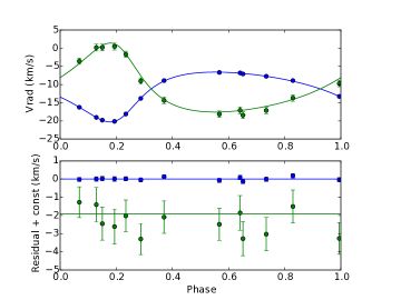
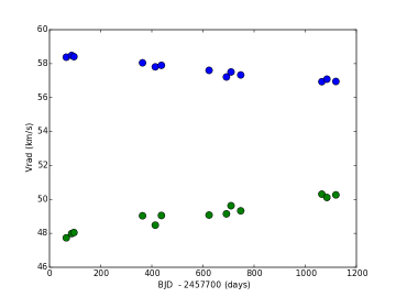
Figure 3: The orbital fit of GJ 1029AB (left) and the radial velocities of L 870-44AB (right).

4.3.2 GJ 1029AB

An orbit for this system was reported in Baroch et al. (2018); we independently detected the presence of doubled lines in 2017 and proceeded to measure the orbit. We gathered 15 spectra with S/N per spectral resolution element of 13-21. We see negligible rotational broadening. We discarded two epochs with insufficient velocity separation, and used a light ratio of 0.223 to calculate the velocities. We find an orbital period of $95.76\pm 0.18$ days, in agreement with the period reported in Baroch et al. (2018). We measure an eccentricity of $0.3786\pm 0.0067$ and a mass ratio of $0.722\pm 0.026$. We show the resulting orbital fit in the right panel of Figure 3.

4.3.3 L 870-44AB

This system was included in our initial sample with a photometric distance of 14.6$\pm$2.2 pc (Winters et al., 2015), but the Gaia DR2 reports a trigonometric distance of 25.6$\pm$0.7 pc. Jódar et al. (2013) reported a visual companion detected with lucky imaging to have an angular separation of 0$\farcs$238 at a position angle of 189° in 2008 with a $\Delta$ $I$ of 1.37 mag between the components.

We report the detection of double lines in the spectrum of this object and a long-term trend in the velocities. With twelve spectra of S/N per spectral resolution element of 16-34 taken over nearly three years, we estimate the orbital period of this system to be roughly 19 years. This is in agreement with the roughly 18-year orbital period we estimate from the lucky imaging results, assuming a circular orbit with a semi-major axis equal to the angular separation. The flux ratio of 0.369 derived from our TODCOR analysis of the spectra near 710 nm is roughly in agreement with the reported magnitude difference at $I$ in Jódar et al. (2013) (corresponding to a flux ratio of 0.28), so we are confident that the component observed in our spectra is the same. Neither component show detectable rotational broadening. Using the Wilson method, we derive a mass ratio of $0.60\pm 0.05$ and a gamma velocity of $54.4\pm 1.5$ km s^-1. We do not report an orbit for this system; thus, we do not report uncertainties on the RVs. We show the RVs of the components as a function of time in the right panel of Figure 3, and we include our measured radial velocities, without uncertainties, in Table 3.

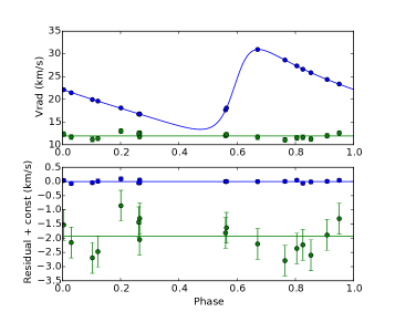
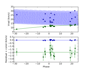
Figure 4: The folded (left) and unfolded (right) orbital fits of LTT 11586AcB, where the unfolded orbit illustrates the velocity drift, modeled as a quadratic, of the outer ‘B’ component.

4.3.4 LTT 11586AcB

This is a known triple system, which is reported to be an SB1 (Jeffers et al., 2018) with a visual component resolved with lucky imaging (Cortés-Contreras et al., 2017) with a $\Delta$ $I_{\rm KC}$ of $1.96\pm 0.05$ mag at a separation of $0\farcs 540\pm 0\farcs 003$. We confirm that it is a triple system where we see doubled spectral lines and present the orbit of the inner SB1 here. We refer to the primary component as ‘A’, the widely separated component, whose spectral lines we detect, as ‘B’, and the primary’s unseen companion as ‘c’.

We obtained 20 spectra of this system with S/N per spectral resolution element of 15-41. We estimate masses for A and B by converting the $\Delta$ $I_{\rm KC}$ to $\Delta$ $K_{\rm s}$ using the relations in Riedel et al. (2014) and then using the MLR by Benedict et al. (2016). We find masses for A and B of $0.289\pm 0.017$ and $0.134\pm 0.014$ M/M_⊙. We determine a light ratio of 0.202 between A and B and use a rotational velocity of 4 km s^-1 for the B to calculate the velocities of A and B, constraining the velocities of B to be between 8 and 15 km s^-1. We fit a quadratic drift ($\ddot{\gamma}$) to B and discarded three observations with insufficient velocity separation between A and B. We find an orbital period of $15.04547\pm 0.00041$ days, an eccentricity of $0.5029\pm 0.0055$, and a minimum mass ratio of $0.1462\pm 0.0014$ for the SB1. The unseen component of the SB1, c, for which we measure a minimum mass of $44.27\pm 0.44$ M_J, is significantly below the stellar-substellar boundary. We show the orbit in the left panel of Figure 4. We also show the unfolded orbit in the right panel to illustrate the velocity drift of the outer B component in the system. We do not report velocity uncertainties for the B component; the uncertainties shown in the orbital fits for this component are the rms of the velocities.

We calculate a mass ratio of $0.40\pm 0.02$ for B/Ac. Assuming a circular orbit and a semi-major axis between Ac and B equal to the reported angular separation in Cortés-Contreras et al. (2017), we estimate an orbital period for B around Ac of 23 years.

4.3.5 2MA 0930+0227AB

This new double-lined spectroscopic binary had no existing spectrum in the literature when it was added to our target list. We detected a faint secondary that had significant rotation and gathered 25 spectra of the system with S/N per spectral resolution element of 15-28. We adopted a light ratio of 0.404 to calculate the radial velocities with rotational velocities of 3 and 26 km s^-1 for the primary and secondary components, respectively. We determine an orbital period of $916.8\pm 2.5$ days, an eccentricity of $0.1928\pm 0.0046$, and a mass ratio of $0.667\pm 0.035$ for 2MA 0930+0227AB. We show the orbital solution to the TRES data in the left panel of Figure 5. We note that the residuals to the fit of the B component’s velocities are large due to the faintness and large rotational broadening of the component.

4.3.6 LP 734-34AB

This new double-lined spectroscopic binary had no existing spectrum or parallax in the literature when it was added to our target list. We acquired 24 spectra of LP 734-34AB with a S/N per spectral resolution element of 8-29. We estimate a light ratio of 0.905 to derive the velocities with negligible broadening. The removal of six epochs with poorly-separated velocities, as well as the flipping of the components’ velocities for the ninth, eleventh, and sixteenth observations, yields a sensible fit for the orbit, which we show in the right panel of Figure 5. We find an orbital period of $33.6551\pm 0.0046$ days, an eccentricity of $0.423\pm 0.010$, and a mass ratio of $0.956\pm 0.010$ for this system.

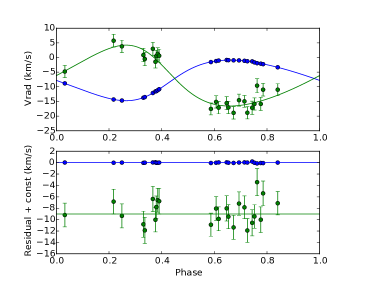
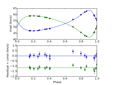
Figure 5: The orbits of 2MA 0930+0227AB (left) and LP 734-34AB (right).

4.3.7 GJ 1182AB

This object was noted in Jenkins et al. (2009) as having a possible binary component, and an orbit for this system was reported in Baroch et al. (2018). As with GJ 1029, we independently discovered this double-lined system in 2017 and began measuring the orbit. We obtained 17 spectra of GJ 1182AB with S/N per spectral resolution element of 11-24 from which we derive a light ratio of 0.197 with no correction for rotational broadening applied. We discarded three epochs with insufficient velocity separation, and measure a $154.23\pm 0.51$-day orbital period, in agreement with that reported in Baroch et al. (2018). We find an eccentricity of $0.5362\pm 0.0022$ and a mass ratio of $0.6606\pm 0.0095$ for this system. We show the orbit in the left panel of Figure 6.

4.3.8 G 258-17AB

G 258-17 is a wide companion to the more massive star HD 161897 and is found at an angular separation of 89$\farcs$8 at a position angle of 28.3° from the primary, as noted by Tokovinin (2014). We initially overlooked an existing $Hipparcos$ parallax (van Leeuwen, 2007) for HD 161897 of $33.30\pm 0.47$ mas and included the star in our sample based on the parallax by Dittmann et al. (2014); however, the Gaia DR2 parallax for G 258-17 of $33.5254\pm 0.0492$ mas is in agreement with that by van Leeuwen (2007). We report the discovery of a near-equal luminosity companion to G 258-17, making the system a hierarchical triple. We acquired 11 spectra of G 258-17AB with a S/N per spectral resolution element of 19-32. We see negligible rotational broadening in the spectra and use a flux ratio of 0.986 to calculate the velocities. We omitted one epoch due to insufficient velocity separation between the components. Because todcor can sometimes confuse components in nearly-equal-luminosity systems, we reversed the velocities of the components for the first, third, and fourth observations, assuming that the brightest component was the primary. We find an orbital period of $4.741475\pm 0.000018$ days, an eccentricity of $0.00495\pm 0.00096$, and a mass ratio of $1.0003\pm 0.0019$. We show our orbital fit to the velocities in the right panel of Figure 6.

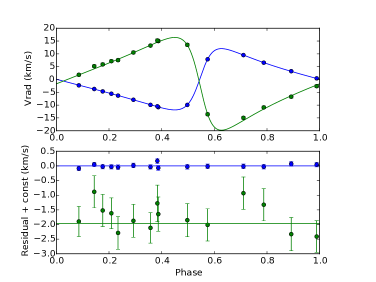
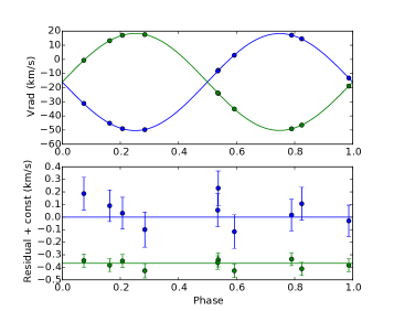
Figure 6: The orbital fits of GJ 1182AB (left) and G 258-17AB (right).

4.3.9 LTT 7077AB

This object was not initially included in our sample because, although it is nearer than 15 pc, the estimated mass of the primary from $M_{K}$ is 0.35 M_⊙. However, this system was noted by Malo et al. (2014) to be a double-lined spectroscopic binary, so we chose to observe this system under the assumption that a deblended $K$ magnitude and/or a measured orbit would result in a primary mass within our range of interest. We obtained 17 spectra of LTT 7077AB with S/N per spectral resolution element of 6-21. We assumed zero rotational broadening and find a light ratio of 0.901. We discarded two data points because the velocities were not widely separated and reversed the components’ velocities for the first observation. We measure an orbital period of $83.926\pm 0.032$ days, an eccentricity of $0.0640\pm 0.0021$, and a mass ratio of $0.9341\pm 0.0031$ for LTT 7077AB. We show the orbit in the left panel of Figure 7.

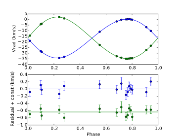
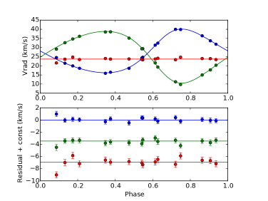
Figure 7: The orbital fits of LTT 7077AB (left) and LP 655-43ABC (right).

4.4 Triple-lined System: LP 655-43ABC

This is a new triple-lined system. We gathered 16 spectra of LP 655-43ABC with S/N per spectral resolution element of 13-26. The three components are resolved for only three epochs. We derive a light ratio of 0.76 for the secondary-to-primary pair of components and 0.40 for the tertiary-to-primary pair, which we used to calculate the velocities. We fix the velocities for the third component to be between 22 and 26 km s^-1. We see negligible rotational broadening for any of the components. We measure for LP 655-43AB an orbital period of $18.3715\pm 0.0084$ days, an eccentricity of $0.1994\pm 0.0078$, and a mass ratio of $0.844\pm 0.014$. We show the orbit in Figure 7. The velocity uncertainties for the C component shown in Figure 7 are the standard deviation of the calculated velocities, as we did not fit this component in our MCMC analysis. A photometric rotation period reported by Newton et al. (2018) of 18.38 days, in agreement with the orbital period of 18.38 days for the inner SB2, indicates that the orbit of the inner pair has synchronized.

Because the velocities of the C component do not significantly vary, we also compared the POSS-1 red plate image taken 1953.933 to the UK Schmidt $I-$band image taken 2001.804 to ensure that the SB2 had not moved on top of a background star. No other star is seen at the current position of the system. In addition, there is only one Gaia DR2 data point at the location of the system, so C is not a background star with a separate (and discrepant) parallax.

Table 5: Orbital Elements for Binaries

Name	MCMC Parameter	MCMC Value	Derived Parameter	Derived Value
GJ 1029AB
	$e\cos\omega$	$-0.3280\pm 0.0069$	$e$	$0.3786\pm 0.0067$
	$e\sin\omega$	$-0.1891\pm 0.0084$	$\omega$ (deg)	$210.0\pm 1.3$
	$T_{0}$ (BJD)	$2457741.08\pm 0.56$	$a\sin i$ (AU)	$0.1331\pm 0.0027$
	$P$ (days)	$95.76\pm 0.18$	$(M_{1}+M_{2})\sin^{3}i$ (${\rm M}_{\odot}$)	$0.03430\pm 0.00210$
	$q$	$0.722\pm 0.026$	$M_{1}\sin^{3}i$ (${\rm M}_{\odot}$)	$0.01991\pm 0.00150$
	$\gamma$ (km s-1)	$-11.189\pm 0.036$	$M_{2}\sin^{3}i$ (${\rm M}_{\odot}$)	$0.01439\pm 0.00061$
	$(K_{1}+K_{2})$ (km s-1)	$16.34\pm 0.34$	$T_{\rm peri}$ (BJD)	$2457761.58\pm 0.54$
	$\sigma_{1}$ (km s-1)	$0.099\pm 0.028$	$\cdots$	$\cdots$
	$\sigma_{2}$ (km s-1)	$0.774\pm 0.161$	${\alpha}_{ast}$ (mas)	$4.6$
LP 655-43AB
	$e\cos\omega$	$0.1324\pm 0.0082$	$e$	$0.1994\pm 0.0078$
	$e\sin\omega$	$-0.1487\pm 0.0088$	$\omega$ (deg)	$311.7\pm 2.7$
	$T_{0}$ (BJD)	$2458036.080\pm 0.069$	$a\sin i$ (AU)	$0.04322\pm 0.00036$
	$P$ (days)	$18.3715\pm 0.0084$	$(M_{1}+M_{2})\sin^{3}i$ (${\rm M}_{\odot}$)	$0.03191\pm 0.00080$
	$q$	$0.844\pm 0.014$	$M_{1}\sin^{3}i$ (${\rm M}_{\odot}$)	$0.01731\pm 0.00046$
	$\gamma$ (km s-1)	$26.550\pm 0.072$	$M_{2}\sin^{3}i$ (${\rm M}_{\odot}$)	$0.01460\pm 0.00038$
	$(K_{1}+K_{2})$ (km s-1)	$26.12\pm 0.22$	$T_{\rm peri}$ (BJD)	$2458029.89\pm 0.12$
	$\sigma_{1}$ (km s-1)	$0.288\pm 0.060$	$\cdots$	$\cdots$
	$\sigma_{2}$ (km s-1)	$0.339\pm 0.071$	${\alpha}_{ast}$ (mas)	0.2
LTT 11586Ac
	$e\cos\omega$	$0.1202\pm 0.0090$	$e$	$0.5029\pm 0.0055$
	$e\sin\omega$	$-0.4882\pm 0.0074$	$\omega$ (deg)	$283.8\pm 1.2$
	$T_{0}$ (BJD)	$2458108.670\pm 0.073$	$T_{\rm peri}$ (BJD)	$2458102.629\pm 0.039$
	$P$ (days)	$15.04547\pm 0.00041$	$a_{1}\sin i$ (AU)	$0.010529\pm 0.000095$
	$\gamma$ (km s-1)	$21.112\pm 0.024$	$f_{1}(M)$ (${\rm M}_{\odot}$)	$0.000688\pm 0.000019$
	$\dot{\gamma}$ (km s-1 day-1)	$-0.002323\pm 0.000093$	$q_{\rm min}$	$0.1462\pm 0.0014$
	$\ddot{\gamma}$ (km s-1 day-1 day-1)	$0.00000172\pm 0.00000035$	$a_{\rm min}$ (AU)	$0.082527\pm 0.000035$
	$K$ (km s-1)	$8.81\pm 0.11$	$M_{2,{\rm min}}$ (${\rm M}_{\odot}$)	$0.04226\pm 0.00042$
	$\sigma$ (km s-1)	$0.058\pm 0.014$	$M_{2,{\rm min}}$ (${\rm M}_{\rm Jup}$)	$44.27\pm 0.44$
	$\cdots$	$\cdots$	${\alpha}_{ast}$ (mas)	$>0.1$
LHS 1817Ab
	$e\cos\omega$	$-0.0002\pm 0.0033$	$e$	$0.0063\pm 0.0031$
	$e\sin\omega$	$0.0053\pm 0.0032$	$\omega$ (deg)	$93\pm 37$
	$T_{0}$ (BJD)	$2458357.72859\pm 0.00029$	$T_{\rm peri}$ (BJD)	$2458357.731\pm 0.032$
	$P$ (days)	$0.30992678\pm 0.00000048$	$a_{1}\sin i$ (AU)	$0.0035702\pm 0.0000089$
	$\gamma$ (km s-1)	$-0.71\pm 0.35$	$f_{1}(M)$ (${\rm M}_{\odot}$)	$0.06321\pm 0.00048$
	$K$ (km s-1)	$125.33\pm 0.31$	$q_{\rm min}$	$0.9343\pm 0.0035$
	$\sigma$ (km -1)	$0.75\pm 0.11$	$a_{\rm min}$ (AU)	$0.0073917\pm 0.0000044$
	$\cdots$	$\cdots$	$M_{2,{\rm min}}$ (${\rm M}_{\odot}$)	$0.2709\pm 0.0010$
	$\cdots$	$\cdots$	$M_{2,{\rm min}}$ (${\rm M}_{\rm Jup}$)	$283.8\pm 1.0$
	$\cdots$	$\cdots$	${\alpha}_{ast}$ (mas)	$>0.1$
2MA 0930$+$0227AB
	$e\cos\omega$	$-0.0950\pm 0.0048$	$e$	$0.1928\pm 0.0046$
	$e\sin\omega$	$-0.1677\pm 0.0037$	$\omega$ (deg)	$240.5\pm 1.2$
	$T_{0}$ (BJD)	$2457910.7\pm 2.6$	$a\sin i$ (AU)	$1.433\pm 0.045$
	$P$ (days)	$916.8\pm 2.5$	$(M_{1}+M_{2})\sin^{3}i$ (${\rm M}_{\odot}$)	$0.467\pm 0.044$
	$q$	$0.667\pm 0.035$	$M_{1}\sin^{3}i$ (${\rm M}_{\odot}$)	$0.280\pm 0.032$
	$\gamma$ (km s-1)	$-7.161\pm 0.025$	$M_{2}\sin^{3}i$ (${\rm M}_{\odot}$)	$0.187\pm 0.012$
	$(K_{1}+K_{2})$ (km s-1)	$17.32\pm 0.54$	$T_{\rm peri}$ (BJD)	$2458262.3\pm 2.6$
	$\sigma_{1}$ (km s-1)	$0.0580\pm 0.0094$	$\cdots$	$\cdots$
	$\sigma_{2}$ (km s-1)	$1.8149\pm 0.2633$	${\alpha}_{ast}$ (mas)	$7$
LP 734-34AB
	$e\cos\omega$	$0.2839\pm 0.0092$	$e$	$0.423\pm 0.010$
	$e\sin\omega$	$0.3139\pm 0.0080$	$\omega$ (deg)	$47.89\pm 0.93$
	$T_{0}$ (BJD)	$2457868.220\pm 0.066$	$a\sin i$ (AU)	$0.04786\pm 0.00034$
	$P$ (days)	$33.6551\pm 0.0046$	$(M_{1}+M_{2})\sin^{3}i$ (${\rm M}_{\odot}$)	$0.01292\pm 0.00028$
	$q$	$0.956\pm 0.010$	$M_{1}\sin^{3}i$ (${\rm M}_{\odot}$)	$0.00661\pm 0.00014$
	$\gamma$ (km s-1)	$52.890\pm 0.031$	$M_{2}\sin^{3}i$ (${\rm M}_{\odot}$)	$0.00631\pm 0.00014$
	$(K_{1}+K_{2})$ (km s-1)	$17.08\pm 0.19$	$T_{\rm peri}$ (BJD)	$2457866.693\pm 0.061$
	$\sigma_{1}$ (km s-1)	$0.156\pm 0.036$	$\cdots$	$\cdots$
	$\sigma_{2}$ (km s-1)	$0.128\pm 0.031$	${\alpha}_{ast}$ (mas)	$0.1$
G 123-45Ab
	$e\cos\omega$	$-0.1153\pm 0.0022$	$e$	$0.3758\pm 0.0024$
	$e\sin\omega$	$0.3577\pm 0.0025$	$\omega$ (deg)	$107.86\pm 0.35$
	$T_{0}$ (BJD)	$2457754.486\pm 0.063$	$T_{\rm peri}$ (BJD)	$2457755.218\pm 0.069$
	$P$ (days)	$34.7557\pm 0.0041$	$a_{1}\sin i$ (AU)	$0.021874\pm 0.000046$
	$\gamma$ (km s-1)	$7.431\pm 0.012$	$f_{1}(M)$ (${\rm M}_{\odot}$)	$0.0011559\pm 0.0000073$
	$K$ (km s-1)	$7.388\pm 0.017$	$q_{\rm min}$	$0.20903\pm 0.00049$
	$\sigma$ (km s-1)	$0.0382\pm 0.0075$	$a_{\rm min}$ (AU)	$0.126519\pm 0.000020$
	$\cdots$	$\cdots$	$M_{2,{\rm min}}$ (${\rm M}_{\odot}$)	$0.038671\pm 0.000091$
	$\cdots$	$\cdots$	$M_{2,{\rm min}}$ (${\rm M}_{\rm Jup}$)	$40.510\pm 0.096$
	$\cdots$	$\cdots$	${\alpha}_{ast}$ (mas)	$>0.3$
GJ 1182AB
	$e\cos\omega$	$0.0593\pm 0.0055$	$e$	$0.5362\pm 0.0022$
	$e\sin\omega$	$-0.5329\pm 0.0021$	$\omega$ (deg)	$276.35\pm 0.58$
	$T_{0}$ (BJD)	$2457782.9\pm 1.6$	$a\sin i$ (AU)	$0.3596\pm 0.0040$
	$P$ (days)	$154.23\pm 0.51$	$(M_{1}+M_{2})\sin^{3}i$ (${\rm M}_{\odot}$)	$0.2608\pm 0.0077$
	$q$	$0.6606\pm 0.0095$	$M_{1}\sin^{3}i$ (${\rm M}_{\odot}$)	$0.1570\pm 0.0054$
	$\gamma$ (km -1)	$-0.625\pm 0.041$	$M_{2}\sin^{3}i$ (${\rm M}_{\odot}$)	$0.1038\pm 0.0023$
	$(K_{1}+K_{2})$ (km -1)	$30.05\pm 0.29$	$T_{\rm peri}$ (BJD)	$2457713.3\pm 1.5$
	$\sigma_{1}$ (km -1)	$0.068\pm 0.017$	$\cdots$	$\cdots$
	$\sigma_{2}$ (km -1)	$0.484\pm 0.099$	${\alpha}_{ast}$ (mas)	$5.8$
G 258-17AB
	$e\cos\omega$	$-0.00118\pm 0.00070$	$e$	$0.00495\pm 0.00096$
	$e\sin\omega$	$-0.00475\pm 0.00106$	$\omega$ (deg)	$256.0\pm 9.5$
	$T_{0}$ (BJD)	$2457826.5789\pm 0.0017$	$a\sin i$ (AU)	$0.029903\pm 0.000034$
	$P$ (days)	$4.741475\pm 0.000018$	$(M_{1}+M_{2})\sin^{3}i$ (${\rm M}_{\odot}$)	$0.15866\pm 0.00053$
	$q$	$1.0003\pm 0.0019$	$M_{1}\sin^{3}i$ (${\rm M}_{\odot}$)	$0.07932\pm 0.00023$
	$\gamma$ (km -1)	$-16.019\pm 0.018$	$M_{2}\sin^{3}i$ (${\rm M}_{\odot}$)	$0.07934\pm 0.00032$
	$(K_{1}+K_{2})$ (km -1)	$68.608\pm 0.077$	$T_{\rm peri}$ (BJD)	$2457828.76\pm 0.13$
	$\sigma_{1}$ (km -1)	$0.117\pm 0.031$	$\cdots$	$\cdots$
	$\sigma_{2}$ (km -1)	$0.048\pm 0.017$	${\alpha}_{ast}$ (mas)	$\cdots$
LTT 7077AB
	$e\cos\omega$	$-0.0186\pm 0.0019$	$e$	$0.0640\pm 0.0021$
	$e\sin\omega$	$0.0612\pm 0.0021$	$\omega$ (deg)	$106.9\pm 1.6$
	$T_{0}$ (BJD)	$2458290.87\pm 0.12$	$a\sin i$ (AU)	$0.27559\pm 0.00048$
	$P$ (days)	$83.926\pm 0.032$	$(M_{1}+M_{2})\sin^{3}i$ (${\rm M}_{\odot}$)	$0.3964\pm 0.0020$
	$q$	$0.9341\pm 0.0031$	$M_{1}\sin^{3}i$ (${\rm M}_{\odot}$)	$0.2049\pm 0.0011$
	$\gamma$ (km s-1)	$-16.661\pm 0.023$	$M_{2}\sin^{3}i$ (${\rm M}_{\odot}$)	$0.1915\pm 0.0011$
	$(K_{1}+K_{2})$ (km s-1)	$35.795\pm 0.062$	$T_{\rm peri}$ (BJD)	$2458294.34\pm 0.38$
	$\sigma_{1}$ (km s-1)	$0.102\pm 0.021$	$\cdots$	$\cdots$
	$\sigma_{2}$ (km s-1)	$0.092\pm 0.020$	${\alpha}_{ast}$ (mas)	$0.5$

Note. — The uncertainty on the systemic velocity $\gamma$ for each system does not include the systematic uncertainty of 0.5 km s^-1 from the Barnard’s Star template radial velocity, which should be added in quadrature when calculating the total uncertainty on $\gamma$.

5 Discussion

We have measured the spectroscopic orbits of eleven binaries with mid-to-late M dwarf components, including the well-known SB2 GJ 268AB. Within 15 pc, we contribute to the currently known M dwarf multiples population orbital parameters for two new possible brown dwarf and one new M dwarf companion in three systems (G 123-45, LTT 11586, LTT 7077). At distances 15-25 pc, we add system parameters for a new white dwarf and two new M dwarf components in three systems (LHS 1817, 2MA 0930, LP 734-34). And beyond 25 pc, we contribute orbital parameters for two new M dwarf companions in two systems (G 258-17, LP 655-43). In addition, we present RVs for the components of L 870-44 and for the B and C components of LTT 11586 and LP 655-43, respectively.

If the three possible sub-stellar components that we have discovered to-date (including LHS 1610b, which we reported in Winters et al. (2018)) are found to be indeed sub-stellar-mass objects, this would represent a doubling from 0.8% (3/376) to 1.6% (6/376) in the number of mid-to-late M dwarf primaries known to host brown dwarf companions within 15 pc. It is likely that they eluded detection because previous radial velocity surveys of these types of stars have typically obtained only a single observation.

Our discovery of a new, nearby, white dwarf - M dwarf system (LHS 1817Ab) provides an intriguing glimpse into stellar evolution. The M dwarf is unlikely to have been able to survive the violent environment that resulted in the creation of the white dwarf at the current separation ($a_{\rm min}=0.00766$ AU). Thus, the system evolved to the observed configuration over time. This system joins the rare examples of nearby M dwarf - white dwarf systems, a combination found to-date in only 2% of the known multiple systems with M dwarf primaries within 25 pc (Winters et al., 2019). The white dwarf component is a new member of the white dwarf population within 25 pc (Holberg et al., 2016; Subasavage et al., 2017; Hollands et al., 2018).

Some of the new systems presented here will be benchmark systems because of the possibility of deriving the true masses for the components. While recent results from the Robo-AO survey indicate that the Gaia DR2 does not resolve binaries with separations less than roughly 1″ (Ziegler et al., 2018), the final Gaia data release will publish astrometric orbits for binary systems. We therefore estimate in the $R_{\sc KC}$ filter the magnitudes of the astrometric perturbations ${\alpha}_{ast}$ of the systems reported here. For double-lined systems, we begin with an estimated $\Delta K$ magnitude between the components. We then varied the magnitude difference and calculated the component masses using the MLR by Benedict et al. (2016) and the resulting mass ratio until it agreed with the mass ratio from our orbital solution. We then converted the final $\Delta K$ to $\Delta R_{\sc KC}$ using the relations in Riedel et al. (2014) and followed the prescription in van de Kamp (1975) to calculate the magnitude of the astrometric perturbation. For the single-lined systems, we use $q_{min}$, $a_{1}\sin i$ converted to arcseconds via the parallax, and assume a $\Delta K$ of 10 magnitudes. Thus, our estimates for the single-lined systems are lower limits. We estimate the magnitudes of astrometric perturbations for our systems to range between 0.0 mas to 7.0 mas and list them in Table 5. The astrometric perturbations of the near-equal-mass systems with small separations between components (LP 734-34 and G 258-17) will likely not be detected by Gaia, as the shift in the position of the photocenter is below the anticipated astrometric precision for binaries with small magnitude differences between the components (0.2 mas; Lindegren et al., 2018). GJ 1029, GJ 268, 2MA 0930, GJ 1182, and LTT 7077 have estimated perturbations of 4.6, 0.7, 7.0, 5.8, and 0.5 mas, respectively. These will be benchmark systems, as the astrometric orbital solutions from Gaia will provide the orbital inclinations that will enable the calculation of the true masses of each component.

The orbits that we have measured help to fill in some of the gaps in our knowledge of the period, separation, eccentricity, and mass ratio distributions for M dwarf multiple stars. Duchêne & Kraus (2013) find that the separation distribution for M dwarfs across all spectral sub-types peaks at 5.3 AU, whereas recent results from Winters et al. (2019) found peaks of 4 AU and 20 AU for the volume-limited 10 pc and 25 pc M dwarf samples, respectively. The true answer is likely closer to 5 AU, but the closest M dwarfs have not yet been comprehensively surveyed with the multi-epoch, high-resolution techniques necessary to detect companions at such separations. We are resolving this incompleteness with our high-resolution spectroscopic and speckle imaging surveys (Winters et al., in prep). A full analysis of orbital parameter distributions for mid-to-late M dwarfs is beyond the scope of this paper, but will be addressed once the southern hemisphere portion of our spectroscopic survey is complete.

References

- Baroch et al. (2018) Baroch, D., Morales, J. C., Ribas, I., et al. 2018, A&A, 619, A32
- Benedict et al. (1998) Benedict, G. F., McArthur, B., Nelan, E., et al. 1998, AJ, 116, 429
- Benedict et al. (2016) Benedict, G. F., Henry, T. J., Franz, O. G., et al. 2016, AJ, 152, 141
- Bessell & Weis (1987) Bessell, M. S., & Weis, E. W. 1987, PASP, 99, 642
- Boyajian et al. (2012) Boyajian, T. S., von Braun, K., van Belle, G., et al. 2012, ApJ, 757, 112
- Buchhave et al. (2010) Buchhave, L. A., Bakos, G. Á., Hartman, J. D., et al. 2010, ApJ, 720, 1118
- Claret et al. (2012) Claret, A., Hauschildt, P. H., & Witte, S. 2012, A&A, 546, A14
- Cortés-Contreras et al. (2017) Cortés-Contreras, M., Béjar, V. J. S., Caballero, J. A., et al. 2017, A&A, 597, A47
- Davison et al. (2014) Davison, C. L., White, R. J., Jao, W.-C., et al. 2014, AJ, 147, 26
- Delfosse et al. (1999a) Delfosse, X., Forveille, T., Beuzit, J.-L., et al. 1999a, A&A, 344, 897
- Delfosse et al. (1999b) Delfosse, X., Forveille, T., Udry, S., et al. 1999b, A&A, 350, L39
- Dittmann et al. (2014) Dittmann, J. A., Irwin, J. M., Charbonneau, D., & Berta-Thompson, Z. K. 2014, ApJ, 784, 156
- Dittmann et al. (2017) Dittmann, J. A., Irwin, J. M., Charbonneau, D., et al. 2017, Nature, 544, 333
- Donati et al. (1997) Donati, J.-F., Semel, M., Carter, B. D., Rees, D. E., & Collier Cameron, A. 1997, MNRAS, 291, 658
- Duchêne & Kraus (2013) Duchêne, G., & Kraus, A. 2013, ARA&A, 51, 269
- Duquennoy & Mayor (1988) Duquennoy, A., & Mayor, M. 1988, A&A, 200, 135
- Finch et al. (2018) Finch, C. T., Zacharias, N., & Jao, W.-C. 2018, AJ, 155, 176
- Foreman-Mackey et al. (2013) Foreman-Mackey, D., Hogg, D. W., Lang, D., & Goodman, J. 2013, PASP, 125, 306
- Gaia Collaboration et al. (2018) Gaia Collaboration, Brown, A. G. A., Vallenari, A., et al. 2018, A&A, 616, A1
- Gregory (2005) Gregory, P. C. 2005, ApJ, 631, 1198
- Holberg et al. (2016) Holberg, J. B., Oswalt, T. D., Sion, E. M., & McCook, G. P. 2016, MNRAS, 462, 2295
- Hollands et al. (2018) Hollands, M. A., Tremblay, P.-E., Gänsicke, B. T., Gentile-Fusillo, N. P., & Toonen, S. 2018, MNRAS, 480, 3942
- Irwin et al. (2015) Irwin, J. M., Berta-Thompson, Z. K., Charbonneau, D., et al. 2015, in Cambridge Workshop on Cool Stars, Stellar Systems, and the Sun, Vol. 18, 18th Cambridge Workshop on Cool Stars, Stellar Systems, and the Sun, ed. G. T. van Belle & H. C. Harris, 767–772
- Irwin et al. (2011) Irwin, J. M., Quinn, S. N., Berta, Z. K., et al. 2011, ApJ, 742, 123
- Jeffers et al. (2018) Jeffers, S. V., Schöfer, P., Lamert, A., et al. 2018, A&A, 614, A76
- Jenkins et al. (2009) Jenkins, J. S., Ramsey, L. W., Jones, H. R. A., et al. 2009, ApJ, 704, 975
- Jódar et al. (2013) Jódar, E., Pérez-Garrido, A., Díaz-Sánchez, A., et al. 2013, MNRAS, 429, 859
- Kesseli et al. (2018) Kesseli, A. Y., Muirhead, P. S., Mann, A. W., & Mace, G. 2018, AJ, 155, 225
- Kirkpatrick et al. (1991) Kirkpatrick, J. D., Henry, T. J., & McCarthy, Jr., D. W. 1991, ApJS, 77, 417
- Kurtz & Mink (1998) Kurtz, M. J., & Mink, D. J. 1998, PASP, 110, 934
- Lacy (1977) Lacy, C. H. 1977, ApJ, 218, 444
- Latham et al. (2002) Latham, D. W., Stefanik, R. P., Torres, G., et al. 2002, AJ, 124, 1144
- Lindegren et al. (2018) Lindegren, L., Hernández, J., Bombrun, A., et al. 2018, A&A, 616, A2
- Malo et al. (2014) Malo, L., Artigau, É., Doyon, R., et al. 2014, ApJ, 788, 81
- Mann et al. (2015) Mann, A. W., Feiden, G. A., Gaidos, E., Boyajian, T., & von Braun, K. 2015, ApJ, 804, 64
- Mann et al. (2016) —. 2016, ApJ, 819, 87
- Marcy & Benitz (1989) Marcy, G. W., & Benitz, K. J. 1989, ApJ, 344, 441
- Mazeh et al. (2003) Mazeh, T., Simon, M., Prato, L., Markus, B., & Zucker, S. 2003, ApJ, 599, 1344
- Ment et al. (2019) Ment, K., Dittmann, J. A., Astudillo-Defru, N., et al. 2019, AJ, 157, 32
- Newton et al. (2016) Newton, E. R., Irwin, J., Charbonneau, D., et al. 2016, ApJ, 821, 93
- Newton et al. (2018) Newton, E. R., Mondrik, N., Irwin, J., Winters, J. G., & Charbonneau, D. 2018, AJ, 156, 217
- Nidever et al. (2002) Nidever, D. L., Marcy, G. W., Butler, R. P., Fischer, D. A., & Vogt, S. S. 2002, ApJS, 141, 503
- Nutzman & Charbonneau (2008) Nutzman, P., & Charbonneau, D. 2008, PASP, 120, 317
- Raghavan et al. (2010) Raghavan, D., McAlister, H. A., Henry, T. J., et al. 2010, ApJS, 190, 1
- Reid et al. (2002) Reid, I. N., Kilkenny, D., & Cruz, K. L. 2002, AJ, 123, 2822
- Reiners et al. (2018) Reiners, A., Zechmeister, M., Caballero, J. A., et al. 2018, A&A, 612, A49
- Riedel et al. (2014) Riedel, A. R., Finch, C. T., Henry, T. J., et al. 2014, AJ, 147, 85
- Ségransan et al. (2000) Ségransan, D., Delfosse, X., Forveille, T., et al. 2000, A&A, 364, 665
- Shkolnik et al. (2012) Shkolnik, E. L., Anglada-Escudé, G., Liu, M. C., et al. 2012, ApJ, 758, 56
- Shkolnik et al. (2010) Shkolnik, E. L., Hebb, L., Liu, M. C., Reid, I. N., & Collier Cameron, A. 2010, ApJ, 716, 1522
- Shporer (2017) Shporer, A. 2017, PASP, 129, 072001
- Skrutskie et al. (2006) Skrutskie, M. F., Cutri, R. M., Stiening, R., et al. 2006, AJ, 131, 1163
- Subasavage et al. (2017) Subasavage, J. P., Jao, W.-C., Henry, T. J., et al. 2017, AJ, 154, 32
- Tokovinin (2014) Tokovinin, A. 2014, AJ, 147, 87
- Tokovinin (1992) Tokovinin, A. A. 1992, A&A, 256, 121
- Tomkin & Pettersen (1986) Tomkin, J., & Pettersen, B. R. 1986, AJ, 92, 1424
- Tonry & Davis (1979) Tonry, J., & Davis, M. 1979, AJ, 84, 1511
- van Altena et al. (1995) van Altena, W. F., Lee, J. T., & Hoffleit, D. 1995, VizieR Online Data Catalog, 1174, 0
- van de Kamp (1975) van de Kamp, P. 1975, ARA&A, 13, 295
- van Leeuwen (2007) van Leeuwen, F. 2007, A&A, 474, 653
- Ward-Duong et al. (2015) Ward-Duong, K., Patience, J., De Rosa, R. J., et al. 2015, MNRAS, 449, 2618
- Weis (1991) Weis, E. W. 1991, AJ, 102, 1795
- Weis (1996) —. 1996, AJ, 112, 2300
- Weis (1999) —. 1999, AJ, 117, 3021
- Wilson (1941) Wilson, O. C. 1941, ApJ, 93, 29
- Winters et al. (2015) Winters, J. G., Henry, T. J., Lurie, J. C., et al. 2015, AJ, 149, 5
- Winters et al. (2017) Winters, J. G., Sevrinsky, R. A., Jao, W.-C., et al. 2017, AJ, 153, 14
- Winters et al. (2018) Winters, J. G., Irwin, J., Newton, E. R., et al. 2018, AJ, 155, 125
- Winters et al. (2019) Winters, J. G., Henry, T. J., Jao, W.-C., et al. 2019, AJ, 157, 216
- Ziegler et al. (2018) Ziegler, C., Law, N. M., Baranec, C., et al. 2018, AJ, 156, 259
- Zucker & Mazeh (1994) Zucker, S., & Mazeh, T. 1994, ApJ, 420, 806
- Zucker et al. (1995) Zucker, S., Torres, G., & Mazeh, T. 1995, ApJ, 452, 863