Simultaneously exciting two atoms with photon-mediated Raman interaction

Abstract

We propose an approach to simultaneously excite two atoms by using cavity-assisted Raman process in combination with cavity photon-mediated interaction. The system consists of a two-level atom and a $\Lambda$-type or V-type three-level atom, which are coupled together with a cavity mode. Having derived the effective Hamiltonian, we find that under certain circumstances a single photon can simultaneously excite two atoms. In addition, multiple photons and even a classical field can also simultaneously excite two atoms. As an example, we show a scheme to realize our proposal in a circuit QED setup, which is artificial atoms coupled with a cavity. The dynamics and the quantum statistical properties of the process are investigated with experimentally feasible parameters.

I Introduction

The light matter interaction has been an important topic since the foundation of the modern physics R1 ; R2 . Recent activities with the aim for realizing quantum information process add more significance on this area since photons provide a convenient medium to control and couple quantum systems R3 ; R4 ; R5 ; R6 . Among these efforts, two-photon absorption and emission process, where two photons are adsorbed or emitted simultaneously by an atom or a molecule, have been extensively investigated R7 ; R8 . However, the reverse phenomenon, one single photon simultaneously excited two atoms or two atoms jointly emitted one single photon, has been rarely studied. Recently, it is rather remarkable that Luigi Garziano et al. R9 have theoretically demonstrated that one photon can simultaneously excite two or more atoms in ultrastrong-coupling (USC) regime R10 ; R11 ; R12 ; R13 of cavity quantum electrodynamics (QED) R2 . In USC regime where the strength of the coupling between the atom and cavity is comparable to the atom and cavity energy scales, the usual rotating-wave approximation (RWA) R14 ; R15 is no longer valid, and the effect of the counter-rotating terms becomes important. In this condition, one photon simultaneously excite two or more atoms via intermediate virtual states connected by these counter-rotating process, can happen deterministically R9 . However, although a few experiments have recently achieved USC regime in solid-state quantum system R11 ; R12 ; R13 , it is difficult to manipulate and readout the state of the atom and cavity individually in this regime with the existing technology, hindering the observation of this novel phenomenon. In order to get rid of the USC obstacle and excite two atoms with single photon in the conventional strong coupling regime R16 ; R17 , we investigate a model which combines cavity-assisted Raman process with cavity photon-mediated interaction.

Commonly, cavity-assisted Raman process employs two field modes interacting with a three-level atom to induce a two-photon coupling between the field modes and the atom. The two field modes are dubbed the pump mode and stokes mode, respectively. This process has been widely studied both theoretically and experimentally for $\Lambda$-type systems R18 ; R19 ; R20 ; R21 and $\Xi$-type systems R22 ; R23 . In general, a Raman interaction Hamiltonian can be obtained by adiabatically eliminating an auxiliary level of a three-level system, yielding an effective two-level system with two-photon coupling R18 ; R19 ; R24 .

On the other hand, it is well known that the exchange of real or virtual photons between two distant atoms results a photon-mediated interaction, which can be used as a general tool to distribute quantum information among different atoms in quantum information processing R5 ; R6 ; R25 ; R26 . Recently, with the fast progress of solid-state quantum information processing R27 ; R28 ; R29 , people have demonstrated the cavity photon-mediated interaction between two distant artificial atoms R30 ; R31 in the circuit QED system, which is a solid-state version of cavity QED. The cavity photon-mediated interaction between artificial atoms is frequently used to couple two qubits and generate entanglement R32 ; R33 ; R34 .

In this work, by combining the cavity-assisted Raman process with cavity photon-mediated interaction, we propose a new approach to simultaneously excite two atoms in the strong coupling regime of cavity QED. We consider a system of a two-level atom and a $\Lambda$-type or V-type three-level atom off-resonantly coupled to a cavity mode, as shown in Fig. 1. By using a unitary transformation, we have obtained an effective Hamiltonian that reflects the essential physics of the process, a single photon can simultaneously excite two atoms. Furthermore, we generalize above process to different cases and find that multiple photons and even a classical field can simultaneously excite two atoms. In addition, we propose a scheme to realize our proposal in a circuit QED architecture, which consists of two tunable-gap flux qubits R35 ; R36 ; R37 capacitively coupled to a superconducting coplanar waveguide resonator R38 . Using experimentally feasible parameters, we numerically simulate the quantum dynamics of this system. It is found that the quantum statistics of this interesting phenomena may provide insight into the essence of this physical process. In particular, we discuss the time evolution of equal-time second-order correlation function in the present work R9 ; R39 ; R40 .

Contrary to that of Luigi Garziano et al. R9 which requires the ultrastrong coupling, our scheme can be realized in the conventional strong coupling regime, in which the system can be well described by the Jaynes-Cummings (JC) Hamiltonian R14 ; R15 . Therefore, one can accurately manipulate the state of the cavity and the atom individually, and extract the quantum information from this system with high fidelity R29 . By using our scheme, one may easily observe this interesting phenomena with the state-of-art technology.

The rest of this paper is organized as follows. In Sec.II, we introduce our model and derive the effective Hamiltonian. In Sec.III, we generalize the effective Hamiltonian derived in Sec.II, and consider several special cases. In Sec.IV, we show a scheme to realize our proposal in a circuit QED architecture, and give the numerical analysis of the dynamics and quantum statistical properties of the process using experimentally feasible parameters. In Sec.V, we give conclusions of our investigation and point out some potential applications.

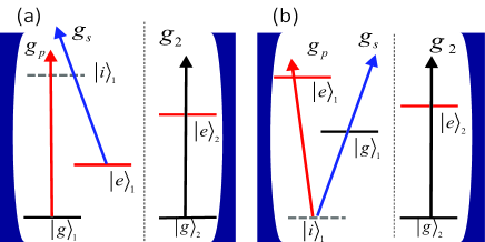
Figure 1: (Color online) Energy level diagram of the system. A system of a two-level atom and a $\Lambda$-type (a) or V-type (b) three-level atom both off-resonantly coupled to a cavity mode. The arrows denotes the coupling between the atom and the cavity mode and the gray dashed line represents the ancillary level in the three-level atom.

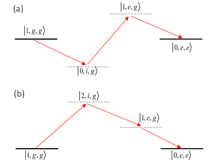
Figure 2: (Color online) Sketch of the process in third-order perturbation theory dominantly contributes to the effective coupling between the bare states $|1,g,g\rangle$ and $|0,e,e\rangle$. (a) and (b) correspond the system depicted in Fig. 1(a) and (b), respectively. The red dashed arrows denote the virtual transitions that doe not conserve the energy, and the gray dashed lines represent the intermediate virtual states.

II the model and hamiltonian

We firstly consider a physical system constituted by a two-level atom and a $\Lambda$-type three-level atom as shown in Fig. 1(a). Both atoms are strongly coupled to a cavity mode. Using the usual RWA, we obtain the Hamiltonian of this system ($\hbar=1$)

$$\begin{aligned} H=H_{0}+H_{I},\end{aligned}$$ (1)

where

$$\begin{aligned} H_{0}=\omega_{c}a^{\dagger}a+\sum_{j=g,e,i}\omega_{j}|j\rangle_{1}\langle j|+\omega_{2}\sigma_{2}^{+}\sigma_{2}^{-},\end{aligned}$$ (2)

contains the energy of a cavity mode, a $\Lambda$-type three-level atom, and a two-level atom, respectively. The second term describes the strong coupling between the two atoms and the cavity mode,

$$\begin{aligned} H_{I}=g_{p}a|i\rangle_{1}\langle g|+g_{s}a|i\rangle_{1}\langle e|+g_{2}a\sigma_{2}^{+}+H.c.,\end{aligned}$$ (3)

here $H.c.$ stands for Hermitian conjugate, $a^{\dagger}$ and $a$ are the creation and annihilation operator for a cavity mode with frequency $\omega_{c}$, respectively. $\sigma_{2}^{\pm}$ are the ladder operators for the two-level atom with transition frequency $\omega_{2}$. $\omega_{j}\,(j=g,e,i)$ is the transition frequency of the three-level atom from ground to excited state $|j\rangle_{1}$. $g_{k}\,(k=p,s,2)$ denotes the coupling strength between the two atoms and the cavity mode. For simplicity, we define $\omega_{g}=0$ in the following discussion.

We consider that the system operates in the dispersive regime, where the atom-cavity detuning is much larger than the coupling strength between them. Then we have $|\Delta_{p}|=|\omega_{i}-\omega_{c}|\gg g_{p},$ $|\Delta_{s}|=|\omega_{i}-\omega_{e}-\omega_{c}|\gg g_{s},$ and $|\Delta_{2}|=|\omega_{2}-\omega_{c}|\gg g_{2}$. The frequency of the cavity mode satisfies $\omega_{c}\approx\omega_{e}+\omega_{2}$. By using the third-order perturbation theory R9 or a unitary transformation R20 ; R41 (The detailed derivation is given in Appendix A), we can write the effective Hamiltonian for our system:

$$\begin{aligned} H_{eff}=&\omega_{c}a^{\dagger}a+\omega_{1}\sigma_{1}^{+}\sigma_{1}^{-}+\omega_{2}\sigma_{2}^{+}\sigma_{2}^{-}\\ &+(\chi a\sigma_{1}^{+}\sigma_{2}^{+}+H.c.),\end{aligned}$$ (4)

where

$$\begin{aligned} \chi=\frac{g_{s}g_{2}}{3}(\frac{1}{\Delta_{s}}+\frac{1}{\Delta_{2}})\frac{g_{p}}{\Delta_{p}}+\frac{g_{p}g_{s}}{3}(\frac{1}{\Delta_{p}}+\frac{1}{\Delta_{s}})\frac{g_{2}}{\Delta_{2}},\end{aligned}$$ (5)

$\sigma_{1}^{\pm}$ are the ladder operators for a reduced two-level system of frequency $\omega_{1}\,(\omega_{e})$ formed by the lowest two levels ($|g\rangle_{1}$ and $|e\rangle_{1}$) of the $\Lambda$-type three-level atom. For simplicity, we have omit the term which constitutes a renormalization of the two atoms and cavity energy levels in Eq. (4) and also throughout the rest of the main text (see the Appendix A, this renormalization of the energy level is a result of dispersive coupling between the atom and the cavity mode). In addition, since the system is operated in the dispersive regime, it is a good approximation to still use the the bare states R59 , which are the eigenstates of the uncoupled Hamiltonian $H_{0}$, instead of the transformed basis (dressed-state basis). We will use this approximation in whole paper. For a physical system constituted by a two-level atom and a V-type three-level atom as shown in Fig. 1(b), we can use same procedure and obtain similar results (see Appendix B).

The last term in Eq. (4), $\chi a\sigma_{1}^{+}\sigma_{2}^{+}+H.c.$, describes a coherent coupling between one photon and two atoms with strength $\chi$. This implies that one can simultaneously excite two atoms with one single cavity photon. As shown in Fig. 2(a), we present the whole process in third-order perturbation theory which leads to the effective coupling between the bare states $|1,g,g\rangle$ and $|0,e,e\rangle.$ For the state vector of the bare state $\left|n,j,k\right\rangle$, the first number denotes the photon number state of the cavity, the second and third entries denote the state of the three-level atom and the two-level atom, respectively. The transition between $|1,g,g\rangle$ and $|0,e,e\rangle$ is connected by three virtual transitions. Fig. 2(b) shows the process for the system depicted in Fig. 1(b).

Although one can obtain the effective coupling between $|1,g,g\rangle$ and $|0,e,e\rangle$ from the perturbation theory, two alternative explanations based on Raman-type process and cavity photon-mediated interaction can better illustrate the mechanism of the process.

(1) The $\Lambda$-type three-level atom is off-resonantly coupled to the cavity mode. This leads to an effective two-photon Raman coupling $a^{\dagger}a(\sigma_{1}^{+}+\sigma_{1}^{-})$ R42 . The coupling strength $J_{a}\sim g_{p}g_{s}(\frac{1}{\Delta_{p}}+\frac{1}{\Delta_{s}})$. Furthermore, exchanging a virtual photon between the reduced two-level atom and the second two-level atom results an effective Hamiltonian $(a\sigma_{1}^{+}\sigma_{2}^{+}+H.c.)$ with coupling strength $\chi_{a}\sim\frac{J_{a}g_{2}}{\Delta_{2}}$.

(2) The cavity photon-mediated interaction between the two atoms results an effective coupling ($a^{\dagger}|g\rangle_{1}\langle i|+H.c.$) R30 ; R41 ; R43 with coupling strength $J_{b}\sim g_{s}g_{2}(\frac{1}{\Delta_{s}}+\frac{1}{\Delta_{2}})$. For the $\Lambda$-type three-level atom, we may think this cavity photon-mediated coupling as atomic-type Stokes mode, and the cavity mode as the pump mode. Therefore, when the three-level system is driven by the two modes, we can adiabatically eliminate the auxiliary level of the three-level atom. Now the three-level atom reduces to an effective two-level atom, and an effective coupling between the two atoms and the cavity mode $(a\sigma_{1}^{+}\sigma_{2}^{+}+H.c.)$ is obtained. The coupling strength is $\chi_{b}\sim\frac{J_{b}g_{p}}{\Delta_{p}}$.

The above two different approaches both include a Raman-type process assisted by the ancillary level $|i\rangle_{1}$ and cavity photon-mediated coupling. It is apparently that the two effective coupling strength $\chi_{a}$ and $\chi_{b}$ correspond to the two terms in Eq. (5). From this qualitative viewpoint, the above process can be easily generalized to the various cases, as shown in the following section.

III simultaneously exciting two atoms: general formulation

In this section, we give a general formulation for the process of simultaneously exciting two atoms.

The physics of a three-level atom interacting with two field modes (quantum or classical) were studied extensively R15 ; R44 . In these systems, cavity-assisted Raman process can leads to two-photon coupling. The Hamiltonian is given by $(a_{p}^{\dagger}a_{s}\sigma^{-}+H.c.)$ for $\Lambda$- or V-type atoms R21 and $(a_{p}^{\dagger}a_{s}^{\dagger}\sigma^{-}+H.c.)$ for $\Xi$-type atoms R22 , where $\sigma^{\pm}$ are the ladder operator for the reduced two-level system, $a_{p}$ and $a_{s}$ are the annihilation operators for the two field modes (the pump mode and the stokes mode), respectively. For the case of classical field mode, one can simply replace the $a_{p}$ or $a_{s}$ with $\epsilon e^{-i(\omega_{d}t+\phi)}$ , where $\epsilon$ and $\phi$ are the real amplitude and phase of the classical field at frequency $\omega_{d}$.

Combining these Raman-assisted two-photon coupling with cavity photon-mediated interaction, we can obtain a general approach to simultaneously excite two atoms.

III.1 two photons simultaneously excite two atoms

Here, we consider the process of two photons exciting two atoms. By jointly absorbing two photons, two atoms are excited from their ground state to the excited state. We noted that in the whole process the single photon can not be absorbed by any one of the two atoms. This resonant interaction between two photons and two atoms can be described with the Hamiltonian (in the interaction picture, and $\hbar=1$),

$$\begin{aligned} H^{I}=\chi_{2}(a)^{2}\sigma_{1}^{+}\sigma_{2}^{+}+H.c.,\end{aligned}$$ (6)

where $a$ $(a^{\dagger})$ is the photon annihilation (creation) operator, $\sigma_{q}^{\pm}(q=1,2)$ are the ladder operators for the $q$th atom, and $\chi_{2}$ denotes the coupling strength.

This effective model can be realized in a system consisting of two three-level atoms. One is $\Lambda$-type and we denote the states as $|g\rangle_{1},|e\rangle_{1},$and $|i\rangle_{1}$. The other is $\Xi$-type and we denote the states as $|g\rangle_{2},|i\rangle_{2},$and $|e\rangle_{2}$. Both atoms are dispersively coupled to a cavity mode. Under the frequency matching condition, by using the fourth-order perturbation theory R9 , we can obtain an effective interaction Hamiltonian, which can be described by Eq. (6). According to fourth-order perturbation theory, the transition between $|2,g,g\rangle$ and $|0,e,e\rangle$ is enabled by paths with four virtual transitions. One trivial example of such path is $|2,g,g\rangle\longrightarrow|1,i,g\rangle\longrightarrow|2,e,g\rangle\longrightarrow|2,e,i\rangle\longrightarrow|2,e,e\rangle$.

Following the same procedure as that used in Sec. II, we give a qualitative explanation of the above effective coupling instead of a full analytical derivation. Firstly, for the two three-level atoms, cavity-assisted Raman process can leads to two-photon coupling interaction, which is given by $a^{\dagger}a(\sigma_{1}^{-}+\sigma_{1}^{+})$ for the $\Lambda$-type atom and $(a^{\dagger})^{2}\sigma_{2}^{-}+(a)^{2}\sigma_{2}^{+}$ for the $\Xi$-type atom. Here $\sigma_{1}^{\pm}$ are the ladder operators for a reduced two-level system formed by the lowest two levels $|g\rangle_{1}$ and $|e\rangle_{1}$ of the $\Lambda$-type three-level atom. $\sigma_{2}^{\pm}$ are the ladder operators acting on the ground and second excited states ($|g\rangle_{2}$ and $|e\rangle_{2}$) of the $\Xi$-type three-level atom. It is apparently that the two reduced two-level atoms are both coupled to a common cavity mode. By exchanging virtual photon with the cavity, a effective coupling between two atoms and two photons is obtained, which can be described by $H_{I}$ in Eq. (6). In fact, since the number of the excitations is conserved in this case, this effective coupling can also be realized in two-atom Tavis-Cummings systemR46 operating in the dispersive regime. According to the second-order perturbation theory, the effective coupling between the states $|2,g,g\rangle$ and $|0,e,e\rangle$ is enabled by paths with two virtual transitions. For example, one of such a path is $|2,g,g\rangle\longrightarrow|1,g,e\rangle\longrightarrow|0,e,e\rangle$.

For multi-photon transitions, we can simply replace $(a^{\dagger})^{2}\sigma_{2}^{-}+(a)^{2}\sigma_{2}^{+}$ with $(a^{\dagger})^{n}\sigma_{2}^{-}+(a)^{n}\sigma_{2}^{+}$. Therefore, we can easily extend the process to the multi-photon case and obtain the effective coupling $a^{n}\sigma_{1}^{+}\sigma_{2}^{+}+H.c$.

III.2 a class field simultaneously excite two atoms

From Eq. (4), we know that in the interaction picture the general Hamiltonian for simultaneously exciting two atoms with one photon is

$$\begin{aligned} H^{I}=\chi(a\sigma_{1}^{+}\sigma_{2}^{+}+H.c.).\end{aligned}$$ (7)

In the parametric approximation, the cavity mode is treated as a classical field without depletion. Thus, by replacing $a$ with $\epsilon e^{-i\phi}$, we transform the Hamiltonian to

$$\begin{aligned} H^{I}=\chi^{\prime}(\sigma_{1}^{+}\sigma_{2}^{+}e^{-i\phi}+H.c.),\end{aligned}$$ (8)

where the effective coupling strength is $\chi^{\prime}=\chi\epsilon$, $\epsilon$ and $\phi$ are the real amplitude and phase of the classical field. For simplicity, we set $\phi=0$ in the following discussion.

This effective model can be realized in a physical system depicted in Fig. 1. However, we need to apply a classical driving field on the three-level atom. This classical driving field is introduced as a classical pump mode. For example, we consider a system depicted in Fig. 1(a). When we apply a classical driving field only on the $\Lambda$-type three-level atom, the Hamiltonian of the system is

$$\begin{aligned} &H=H_{0}+H_{int},\\ &H_{int}=H_{I}+H_{D}\end{aligned}$$ (9)

with $H_{0}$ $(H_{I})$ being given in Eq. (2) (Eq. (3)). The third term comes from the drive of the $\Lambda$-type three-level atom,

$$\begin{aligned} H_{D}=\varepsilon e^{-i\omega_{d}t}|i\rangle_{1}\langle g|+\varepsilon^{\prime}e^{-i\omega_{d}t}|i\rangle_{1}\langle e|+H.c.,\end{aligned}$$ (10)

where $\varepsilon$ and $\varepsilon^{\prime}$ are the real amplitude of the classical driving field with frequency $\omega_{d}$. Then we can rearrange the terms in $H_{int}$, and rewrite $H_{int}$ as

$$\begin{aligned} H_{int}&=(\varepsilon e^{-i\omega_{d}t}|i\rangle_{1}\langle g|+g_{s}a|i\rangle_{1}\langle e|+g_{2}a\sigma_{2}^{+}+H.c.)\\ &+(g_{p}a|i\rangle_{1}\langle g|+\varepsilon^{\prime}e^{-i\omega_{d}t}|i\rangle_{1}\langle e|+H.c.),\end{aligned}$$ (11)

where the terms in the first line have the same form as that of the Hamiltonian in Eq. (3) except replacing the quantum pump mode $(g_{p}a|i\rangle_{1}\langle g|+H.c.)$ with a classical pump mode $(\varepsilon e^{-i\omega_{d}t}|i\rangle_{1}\langle g|+H.c.)$. The terms in the second line have no contribution to the process except shifting the frequency of the energy level in our setting. By analogy with the mechanism discussed in last section, we can simultaneously excite two atoms with a classical driving field.

We still consider that the atom-cavity system operates in the dispersive regime, and the $\Lambda$-type three-level system is off-resonantly driven by the classical field. Then $|\Delta_{d}|=|\omega_{i}-\omega_{d}|\gg\varepsilon$ and $|\Delta_{d}^{\prime}|=|\omega_{i}-\omega_{e}-\omega_{d}|\gg\varepsilon^{\prime}$. The frequency of the classical driving field satisfies $\omega_{d}\approx\omega_{e}+\omega_{2}$. Following the derivation in Sec. II, we can write the effective Hamiltonian in the interaction picture,

$$\begin{aligned} H^{I}_{d}=\chi_{d}(\sigma_{1}^{+}\sigma_{2}^{+}+H.c.),\end{aligned}$$ (12)

where $\sigma_{1}^{\pm}$ are the ladder operators for a reduced two-level system with frequency $\omega_{1}$ formed by the lowest two levels of the $\Lambda$-type three-level atom. The effective coupling strength is

$$\begin{aligned} \chi_{d}=\frac{g_{s}g_{2}}{3}(\frac{1}{\Delta_{s}}+\frac{1}{\Delta_{2}})\frac{\varepsilon}{\Delta_{d}}+\frac{\varepsilon g_{s}}{3}(\frac{1}{\Delta_{d}}+\frac{1}{\Delta_{s}})\frac{g_{2}}{\Delta_{2}}.\end{aligned}$$ (13)

This classical field-induced amplitude- and phase-tunable two-atom coupling can be dubbed the two-photon coherent pump R45 . When the system is initially prepared in the state $|g,g\rangle$, the two-atom GHZ state $(|g,g\rangle+|e,e\rangle)/\sqrt{2}$ can be obtained by applying the classical field on the three level atom after a time $t=\pi/(4\chi_{d})$.

IV physical implementation

With the recent rapid progress in quantum information processing, investigation has been extended from cavity QED systems to circuit QED systems, in which superconducting qubits R47 act as artificial atoms and can strongly interact with a single-mode field at microwave frequencies. The artificial atoms with a long coherence time can be engineered to have different energy level diagrams, including V-type R48 ; R49 , $\Delta$-type R37 , and $\Xi$-type R50 ; R51 . The transition frequency of the atoms can be controlled by a local magnetic flux bias. On the other hand, the superconducting resonator with high quality factor can be easily designed and fabricated with the existing technology. Moreover, one can manipulate the state of the resonator and the artificial atom individually, and read out the states of these system with high fidelity R29 . These features along with the potential of scaling up make the circuit-QED system an attractive platform for studying quantum optics and quantum information processing.

In this section, we show that a single cavity photon can simultaneously excite two atoms in a circuit QED architecture. We numerically simulate the dynamics and quantum statistical properties of the process using experimentally feasible parameters. The numerical calculation were performed using the PYTHON package QuTiP R52 ; R53 .

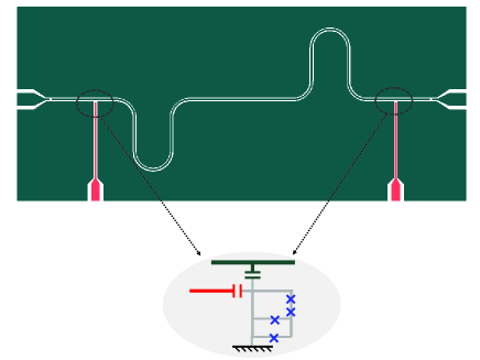
Figure 3: (Color online) Schematic of the superconducting system consisting of two tunable-gap flux qubits with local microwave driving lines (light gray, red online), which are both located in a transmission line resonator (dark gray, green online).

IV.1 implementation in circuit quantum electrodynamics

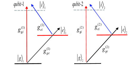
Figure 4: (Color online) Energy level diagram of the two flux qubits. The $\Delta$-type three-level system is off-resonantly coupled to the cavity mode. The present system, which is formed by a pair of identical units (represented by single line and double line, respectively), can be seen as a dimer of the system described in Fig. 1(a). The gray dashed line represents the ancillary level in the three-level system.

As shown in Fig. 3, we consider two tunable-gap flux qubits capacitively coupled to a superconducting coplanar waveguide resonator R36 ; R37 in the strong coupling regime. The flux qubit can be manipulated by a local microwave driving line. To initialized the state of the cavity, we can add an additional frequency tunable qubit (not shown in Fig. 3), which allows us to pump photon into the resonator R54 ; R55 ; R56 . Treating the tunable-gap flux qubit as a $\Delta$-type three-level system and using the usual RWA, we can describe the full system with Hamiltonian ($\hbar=1$)

$$\begin{aligned} &H=\omega_{c}a^{\dagger}a+\sum_{q=1,2}\sum_{j=g,e,i}\omega^{(q)}_{j}|j\rangle_{q}\langle j|+H_{I},\\ &H_{I}=\sum_{q=1,2}a(g^{(q)}_{ge}|e\rangle_{q}\langle g|+g^{(q)}_{gi}|i\rangle_{q}\langle g|+g^{(q)}_{ei}|i\rangle_{q}\langle e|)+H.c,\end{aligned}$$ (14)

where $\omega_{c}$ is cavity frequency, $\omega_{j}^{(q)}$ is the transition frequency from ground state to excited state $|j\rangle_{q}$ of the $q$th flux qubit, and $g_{jk}^{(q)}$ is the qubit-resonator coupling strength for the $q$th flux qubit. For easy reference, we define $\omega_{g}^{(q)}=0$ in the following discussion. We assume that our system operates in the dispersive regime. Then $|\Delta_{2}^{(q)}|=|\omega_{e}^{(q)}-\omega_{c}|\gg g_{ge}^{(q)}$, $|\Delta_{s}^{(q)}|=|\omega_{i}^{(q)}-\omega_{e}^{(q)}-\omega_{c}|\gg g_{ei}^{(q)}$, and $|\Delta_{p}^{(q)}|=|\omega_{i}^{(q)}-\omega_{c}|\gg g_{gi}^{(q)}$. The frequency of the cavity satisfies the frequency matching condition $\omega_{c}\approx\sum_{q=1,2}\omega_{e}^{(q)}$.

As shown in Fig. 4, the present system can be seen as a dimer of the system depicted in Fig. 1(a). Writing out all terms of the summation and rearranging them, one can rewrite $H_{I}$ to

$$\begin{aligned} H_{I}&=(g^{(1)}_{gi}a|i\rangle_{1}\langle g|+g^{(1)}_{ei}a|i\rangle_{1}\langle e|+g^{(2)}_{ge}a|e\rangle_{2}\langle g|+H.c.)\\ &+(g^{(2)}_{gi}a|i\rangle_{2}\langle g|+g^{(2)}_{ei}a|i\rangle_{2}\langle e|+g^{(1)}_{ge}a|e\rangle_{1}\langle g|+H.c.)\end{aligned}$$ (15)

The terms in the first and second line both have the same form as Eq. (3). By analogy with the system discussed in Sec. II, one can also simultaneously excite two atoms with a single cavity photon in this Circuit-QED system. Moreover, it is apparently that except for a path which is the same as that shown in Fig. 2(a), there is another path generating the effective coupling between the states $|1,g,g\rangle$ and $|0,e,e\rangle$ after considering the third-order perturbation. The path is $|1,g,g\rangle\longrightarrow|0,g,i\rangle\longrightarrow|1,g,e\rangle\longrightarrow|0,e,e\rangle$, where $\left|n,j,k\right\rangle$ labels the states of the cavity mode and two three-level systems.

To take into account that our system operates in the dispersive regime, we can eliminate the direct atom-cavity coupling by using the unitary transformation

$$\begin{aligned} U=\exp[\sum_{q=1,2}&\frac{g_{gi}^{(q)}}{\Delta_{p}^{(q)}}a^{\dagger}\left|g\right\rangle_{q}\left\langle i\right|+\frac{g_{ei}^{(q)}}{\Delta_{s}^{(q)}}a^{\dagger}\left|e\right\rangle_{q}\left\langle i\right|\\ &+\frac{g_{ge}^{(q)}}{\Delta_{2}^{(q)}}a^{\dagger}\left|g\right\rangle_{q}\left\langle e\right|-H.c.]\end{aligned}$$ (16)

Following the derivation in Sec. II, we can write the effective Hamiltonian,

$$\begin{aligned} H_{eff}=&\omega_{c}a^{\dagger}a+\omega_{1}\sigma_{1}^{+}\sigma_{1}^{-}+\omega_{2}\sigma_{2}^{+}\sigma_{2}^{-}\\ &+(\chi_{eff}a\sigma_{1}^{+}\sigma_{2}^{+}+H.c.),\end{aligned}$$ (17)

where

$$\begin{aligned} \chi_{eff}=&\frac{g^{(1)}_{ei}g^{(2)}_{ge}}{3}(\frac{1}{\Delta_{s}^{(1)}}+\frac{1}{\Delta_{2}^{(2)}})\frac{g^{(1)}_{gi}}{\Delta_{p}^{(1)}}\\ &+\frac{g^{(1)}_{gi}g^{(1)}_{ei}}{3}(\frac{1}{\Delta_{p}^{(1)}}+\frac{1}{\Delta_{s}^{(1)}})\frac{g^{(2)}_{ge}}{\Delta_{2}^{(2)}}\\ &+\frac{g^{(2)}_{ei}g^{(1)}_{ge}}{3}(\frac{1}{\Delta_{s}^{(2)}}+\frac{1}{\Delta_{2}^{(1)}})\frac{g^{(2)}_{gi}}{\Delta_{p}^{(2)}}\\ &+\frac{g^{(2)}_{gi}g^{(2)}_{ei}}{3}(\frac{1}{\Delta_{p}^{(2)}}+\frac{1}{\Delta_{s}^{(2)}})\frac{g^{(1)}_{ge}}{\Delta_{2}^{(1)}},\end{aligned}$$ (18)

$\sigma_{q}^{\pm}$ are the ladder operators for a qubit formed by the lowest two levels $|g\rangle_{q}$ and $|e\rangle_{q}$ of the $q$th three-level system. The frequency of the qubit is $\omega_{q}.$

IV.2 numerical analysis

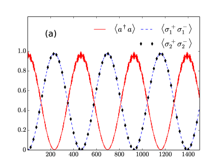
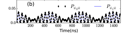
Figure 5: (Color online) Numerical simulation of the nondissipative dynamics. (a) Temporal evolution of the cavity mean photon number $\langle a^{\dagger}a\rangle$ and the qubit mean excitation number $\langle\sigma_{q}^{+}\sigma_{q}^{-}\rangle$ for the initial states $\left|1,g,g\right\rangle$. It can be found that the system undergoes ordinary vacuum Rabi oscillations between $\left|1,g,g\right\rangle$ and $\left|0,e,e\right\rangle$, showing the coherent and reversible excitation exchange between the two qubits and a cavity mode with probability approaching one. This demonstrates that a single photon is absorbed and emitted by the two qubits jointly in a reversible and coherent way. (b) Population leakage to the auxiliary third level of the two three-level systems. In the whole process, the real occupation of the third level is far less than one.

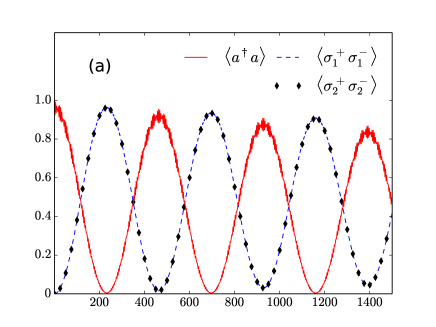
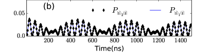
Figure 6: (Color online) Numerical simulation of the dynamics under the influence of dissipation. (a) Temporal evolution of the cavity mean photon number $\langle a^{\dagger}a\rangle$ and the qubit mean excitation number $\langle\sigma_{q}^{+}\sigma_{q}^{-}\rangle$ for the initial states $\left|1,g,g\right\rangle$. (b) Population leakage to the auxiliary third level of the two three-level systems.

To study the feasibility of the proposal, we have performed numerical calculations based on the Hamiltonian in Eq. (14). Note that in the previous effective Hamiltonian in Eq. (17), we do not include analytical expressions for the frequency shifts due to the renormalization and modification caused by the dispersive coupling between the qubit and the cavity mode. However, we take them into account by numerically scanning the cavity frequency to compensate these frequency shift. Therefore, the frequency matching condition can be fulfilled.

For simplicity and without loss of generality, we consider the two tunable-gap flux qubits as two identical $\Delta$-type three-level systems. In what follows, all the numerical analysis are done with the frequencies of cavity and flux qubit, $\omega_{c}/2\pi=7.9655\,GHz$, $\omega_{e}^{(q)}/2\pi=4.00\,GHz$, and $\omega_{i}^{(q)}/2\pi=7.00\,GHz$. The coupling strength are $g_{ge}^{(q)}/2\pi=120\,MHz$, $g_{ei}^{(q)}/2\pi=180\,MHz$, and $g_{gi}^{(q)}/2\pi=100\,MHz$. The cavity photon decay rates and the flux qubit relaxation rates are $\kappa/2\pi=\gamma_{ge}^{(q)}/2\pi=\gamma_{gi}^{(q)}/2\pi=0.01\,MHz$, and $\gamma_{ei}^{(q)}/2\pi=0.015\,MHz$, respectively. Further, we also consider that our system is initially prepared in the state $\left|1,g,g\right\rangle$.

Firstly, we study the dynamics of the system in the absence of dissipation. In Fig. 5, we present the time evolution of the mean photon number $\langle a^{\dagger}a\rangle$ and the qubit mean excitation number $\langle\sigma_{q}^{+}\sigma_{q}^{-}\rangle$. It can be observed from this ordinary oscillation between $\left|1,g,g\right\rangle$ and $\left|0,e,e\right\rangle$ that a single photon is absorbed and emitted by the two qubits jointly with probability approaching one. The period of the oscillation is about 460 $ns$, which is in good agreement with the value calculated based on the effective coupling strength $\chi_{eff}$, $T=\pi/\chi_{eff}=444$ $ns$. Fig. 5(b) shows the population leakage of the auxiliary third level of the two three-level systems. We can find that in the whole process the real occupation of the third level is far less than one.

We now discuss the influence of cavity decay and qubit relaxation on this ongoing physical process. This can be done by solving the master equation (see the Appendix C). In Fig. 6, as expected, the amplitude of the oscillation gets damped due to cavity decay and qubit relaxation. However, one can still observe the oscillation between $\left|1,g,g\right\rangle$ and $\left|0,e,e\right\rangle$.

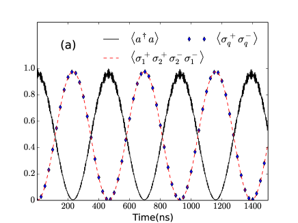
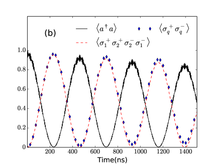
Figure 7: (Color online) Temporal evolution of the the qubit mean excitation number $\langle\sigma_{q}^{+}\sigma_{q}^{-}\rangle$, and the equal-time second-order correlation function $G_{q}^{(2)}=\langle\sigma_{1}^{+}\sigma_{2}^{+}\sigma_{2}^{-}\sigma_{1}^{-}\rangle$ with the system prepared in the state $\left|1,g,g\right\rangle$. (a) shows dynamics in the absence of dissipation and (b) for dynamics under the influence of dissipation. In the nondissipative case, the $\langle\sigma_{q}^{+}\sigma_{q}^{-}\rangle$ and $G_{q}^{(2)}$ almost coincide. This almost perfect two-qubit correlation function is a direct signature that the two qubits are excited jointly. As expected, the oscillation amplitude gets damped under the influence of dissipation. We also observed that the two-qubit correlation function $G_{q}^{(2)}$ goes almost to zero when the cavity mean photon number $\langle a^{\dagger}a\rangle$ is at maximum. This behavior indicates that the photon is not absorbed by a single qubit instead the two qubits jointly.

Most importantly, studying the quantum statistics of this interesting phenomena may provide insight into the essence of this physical process. We particularly focus on the time evolution of equal-time second-order correlation function. In Fig. 7, we display the numerical result of the time evolution of the two-qubit correlation function $G_{q}^{(2)}=\langle\sigma_{1}^{+}\sigma_{2}^{+}\sigma_{2}^{-}\sigma_{1}^{-}\rangle$, which describes the quantum correlation between the emitted photons from the two qubits into noncavity modes R9 . For easy comparison, we also display the numerical result of the time evolution of the qubit mean excitation number $\langle\sigma_{q}^{\dagger}\sigma_{q}^{-}\rangle$ and the mean photon number $\langle a^{\dagger}a\rangle$. We observe that the qubit mean excitation number $\langle\sigma_{q}^{+}\sigma_{q}^{-}\rangle$ and $G_{q}^{(2)}$ almost coincide at any time in the nondissipative case, as shown in Fig. 7(a). This is a signature of almost perfect two-qubit correlation: if one qubit is excited, the other is also excited R9 ; R39 . This behavior indicates that the photon is directly absorbed by the two qubits jointly. Fig. 7(b) shows the influence of dissipation on the time evolution of the equal-time two-qubit correlation function. Compared with the mean qubit excitation number, the equal-time two-qubit correlation function seemes to be more fragile to the system damping. However, during the time evolution, it is notable that the two-qubit correlation function $G_{q}^{(2)}$ goes almost to zero when the cavity mean photon number $\langle a^{\dagger}a\rangle$ is at maximum. This implies that the cavity photon is not absorbed by a single qubit instead the two qubits jointly R40 .

V conclusion

In summary, we have shown that a system consisting of a two-level atom and a $\Lambda$-type or V-type three-level atom off-resonantly coupled to a cavity mode can exhibit anomalous vacuum Rabi oscillations, indicating that two atoms can be simultaneously excited by a single photon and jointly emit a photon into the cavity mode in a reversible and coherent process. Furthermore, we have shown a scheme to realize this interesting phenomena in a circuit QED architecture, and study the quantum statistics of , in particular, the time evolution of equal-time second-order correlation function. Our numerical calculation shows a clear signature that a single photon can be directly absorbed by two atoms simultaneously. In addition, we show that multi-photons and even a classical field can also simultaneously excite two atoms.

These process can be exploited for realizing efficient atom-atom or atom-photon entanglement source R9 . It can also be used for the implementation of novel schemes for the control and manipulation of atomic and cavity states. The resonant coupling between one photon and two atoms may paves the way for investigating multi-atom interaction mediated by cavity photon or multi-qubit mixing process R57 . Although, the model we introduced in this work is at single atom level, one can also apply this model to hybrid quantum system formed by spin or atomic ensemble R58 . This opens up a new possibility for quantum information on hybrid quantum system.

Appendix A

In this appendix, we provide a detailed derivation of the effective Hamiltonian in Eq. (4). We start from the original Hamiltonian in Eq.(1) which is composed of an unperturbed part $H_{0}$ with known eigenvalues and eigenstates and a small perturbation part $H_{I}$. Our system operates in the dispersive regime, where the atom-cavity detuning is larger than the coupling strengths between them. We have $|\Delta_{p}|=|\omega_{i}-\omega_{c}|\gg g_{p},$ $|\Delta_{s}|=|\omega_{i}-\omega_{e}-\omega_{c}|\gg g_{s},$ and $|\Delta_{2}|=|\omega_{2}-\omega_{c}|\gg g_{2}$. The frequency of the cavity mode satisfies the frequency matching condition $\omega_{c}\approx\omega_{e}+\omega_{2}$. For easy reference, we set $\omega_{g}=0$ hereafter.

Considering the system is operated in the dispersive regime, we can eliminate the direct atom-cavity coupling using a unitary transformation

$$\begin{aligned} H_{eff}=e^{-X}He^{X},\end{aligned}$$ (19)

where $X$ is chosen such that the direct coupling between the atom-cavity $H_{I}$ in the transformed Hamiltonian disappear. Here, we choose

$$\begin{aligned} X=\frac{g_{p}}{\Delta_{p}}a^{\dagger}\left|g\right\rangle\left\langle i\right|+\frac{g_{s}}{\Delta_{s}}a^{\dagger}\left|e\right\rangle\left\langle i\right|+\frac{g_{2}}{\Delta_{2}}a^{\dagger}\sigma_{2}^{-}-H.c.,\end{aligned}$$ (20)

so that it satisfies $[H_{0},X]=-H_{I}$. By expanding to the third order of the small parameters ($\frac{g_{p}}{\Delta_{p}},\frac{g_{s}}{\Delta_{s}},\frac{g_{2}}{\Delta_{2}}$), we have

$$\begin{aligned} &e^{-\lambda X}(H_{0}+\lambda H_{I})e^{\lambda X}=(H_{0}+\lambda H_{I})\\ &+\lambda[(H_{0}+\lambda H_{I}),X]+\frac{\lambda^{2}}{2!}[[(H_{0}+\lambda H_{I}),X],X]\\ &+\frac{\lambda^{3}}{3!}[[[(H_{0}+\lambda H_{I}),X],X],X]+O(\lambda^{4})\\ &=H_{0}+\frac{\lambda^{2}}{2}[H_{I},X]+\frac{\lambda^{3}}{3}[[H_{I},X],X]+O(\lambda^{4}),\end{aligned}$$ (21)

where $\lambda$ is introduced to show the orders in the perturbation expansion, and would be set to 1 after the calculations. Under the frequency matching condition, by keeping resonant terms only (in the rotating wave approximation), one can obtain the effective Hamiltonian:

$$\begin{aligned} H_{eff}=&\widetilde{\omega}_{c}a^{\dagger}a+\widetilde{\omega}_{1}\sigma_{1}^{+}\sigma_{1}^{-}+\widetilde{\omega}_{2}\sigma_{2}^{+}\sigma_{2}^{-}+\widetilde{\omega}_{i}|i\rangle_{1}\langle i|\\ &+(\chi a\sigma_{1}^{+}\sigma_{2}^{+}+H.c.),\end{aligned}$$ (22)

where

$$\begin{aligned} \chi=\frac{g_{s}g_{2}}{3}(\frac{1}{\Delta_{s}}+\frac{1}{\Delta_{2}})\frac{g_{p}}{\Delta_{p}}+\frac{g_{s}g_{p}}{3}(\frac{1}{\Delta_{s}}+\frac{1}{\Delta_{p}})\frac{g_{2}}{\Delta_{2}},\end{aligned}$$ (23)

and $\sigma_{1}^{\pm}$ are the ladder operators for a reduced two-level system formed by the lowest two levels ($|g\rangle_{1},|e\rangle_{1}$) of the three-level atom. $\widetilde{\omega}_{c}=\omega_{c}-\frac{g_{p}^{2}}{\Delta_{p}}-\frac{g_{2}^{2}}{\Delta_{2}}$, $\widetilde{\omega}_{2}=\omega_{2}+\frac{g^{2}}{\Delta_{2}}+\frac{2g^{2}}{\Delta_{2}}a^{\dagger}a$ ,$\widetilde{\omega}_{i}=\omega_{i}+(\frac{g_{p}^{2}}{\Delta_{p}}+\frac{g_{s}^{2}}{\Delta_{s}})+(\frac{g_{p}^{2}}{\Delta_{p}}+\frac{g_{s}^{2}}{\Delta_{s}})a^{\dagger}a$, and $\widetilde{\omega}_{1}=\omega_{e}+(\frac{g_{p}^{2}}{\Delta_{p}}-\frac{g_{s}^{2}}{\Delta_{s}})a^{\dagger}a$ are the renormalization transition frequencies of the cavity and two atoms, which is due to atom-cavity dispersive coupling. Since our system is initially prepared in $|1,g,g\rangle$, it is apparently that $|i\rangle_{1}$ is decoupled from our system, leading to a negligible occupation probability on the this level in the whole process. Therefore, we can rewrite the effective Hamiltonian in Eq.(A4)

$$\begin{aligned} H_{eff}=&\widetilde{\omega}_{c}a^{\dagger}a+\widetilde{\omega}_{1}\sigma_{1}^{+}\sigma_{1}^{-}+\widetilde{\omega}_{2}\sigma_{2}^{+}\sigma_{2}^{-}\\ &+(\chi a\sigma_{1}^{+}\sigma_{2}^{+}+H.c.).\end{aligned}$$ (24)

It is worth to point out when we transform Hamiltonian with a unitary operator, the state (basis) also need to be transformed. This means that the operator in Eq. (A4) and Eq. (A6) are the dressed-state operators, i.e., operator represented via dressed-state basis (transformed basis). However, our system operates in the dispersive regime, the dressed-state can be well approximated by the bare states R59 , which are the eigenstates of the uncoupled Hamiltonian $H_{0}$.

Appendix B

Using the similar procedures in section II, we can obtain the effective Hamiltonian of a system consisting of a two-level atom and a V-type three-level atom off-resonantly coupled to a cavity mode as depicted in the Fig. 1(b) of the main text. Similar to the previous procedure, we start from the Hamiltonian ($\hbar=1$),

$$\begin{aligned} &H=H_{0}+H_{I}\\ &H_{0}=\omega_{c}a^{\dagger}a+\sum_{j=g,e,i}\omega_{j}|j\rangle_{1}\langle j|+\omega_{2}\sigma_{2}^{+}\sigma_{2}^{-},\\ &H_{I}=g_{p}a|e\rangle_{1}\langle i|+g_{s}a|g\rangle_{1}\langle i|+g_{2}a\sigma_{2}^{+}+H.c.\end{aligned}$$ (25)

For easy reference, we define $\omega_{i}=0$ hereafter. When atom-cavity detuning are large enough, $|\Delta_{2}|=|\omega_{2}-\omega_{c}|\gg g_{2},|\Delta_{p}|=|\omega_{e}-\omega_{c}|\gg g_{p},$and $|\Delta_{s}|=|\omega_{g}-\omega_{c}|\gg g_{s}$. We can eliminate the direct atom-cavity coupling using the unitary transformation

$$\begin{aligned} &H_{eff}=e^{-S}He^{S},\\ &S=\frac{g_{p}}{\Delta_{p}}a^{\dagger}\left|i\right\rangle\left\langle e\right|+\frac{g_{s}}{\Delta_{s}}a^{\dagger}\left|i\right\rangle\left\langle g\right|+\frac{g_{2}}{\Delta_{2}}a^{\dagger}\sigma_{2}^{-}-H.c.,\end{aligned}$$ (26)

where $S$ satisfies $[H_{0},S]=-H_{I}$. Further, we assume that the frequency of the cavity mode is $\omega_{c}\approx\omega_{e}-\omega_{g}+\omega_{2}$. Following the same procedure as that in Appendix A, we can obtain an effective Hamiltonian

$$\begin{aligned} H_{eff}=&\widetilde{\omega}_{c}a^{\dagger}a+\widetilde{\omega}_{1}\sigma_{1}^{+}\sigma_{1}^{-}+\widetilde{\omega}_{2}\sigma_{2}^{+}\sigma_{2}^{-}+\\ &+(\chi a\sigma_{1}^{+}\sigma_{2}^{+}+h.c.),\end{aligned}$$ (27)

where

$$\begin{aligned} \chi=\frac{g_{s}g_{p}}{3}(\frac{1}{\Delta_{p}}+\frac{1}{\Delta_{s}})\frac{g_{2}}{\Delta_{2}}+\frac{g_{s}g_{2}}{3}(\frac{1}{\Delta_{s}}+\frac{1}{\Delta_{2}})\frac{g_{p}}{\Delta_{p}}\end{aligned}$$ (28)

is the effective coupling strength between the two atom and cavity, and $\sigma_{1}^{\pm}$ are the ladder operators for a reduced two-level system formed by the two levels ($|g\rangle_{1},|e\rangle_{1}$) of the three-level atom. $\widetilde{\omega}_{c}=\omega_{c}+\frac{g_{s}^{2}}{\Delta_{s}}-\frac{g_{2}^{2}}{\Delta_{2}}$, $\widetilde{\omega}_{2}=\omega_{2}+\frac{g_{2}^{2}}{\Delta_{2}}+\frac{2g_{2}^{2}}{\Delta_{2}}a^{\dagger}a$ and $\widetilde{\omega}_{1}=(\omega_{e}-\omega_{g})+(\frac{g_{p}^{2}}{\Delta_{p}}-\frac{g_{s}^{2}}{\Delta_{s}})+(\frac{g_{p}^{2}}{\Delta_{p}}-\frac{g_{s}^{2}}{\Delta_{s}})a^{\dagger}a$ are the renormalization transition frequencies of the cavity and two atoms. The last term in Eq. (B3) implies that one can simultaneously excite two atoms with one cavity photon in the system depicted in Fig. 1(b).

Appendix C

We study the influence of cavity decay and atom relaxation on the process by solving the master equations. By including cavity decay and atom relaxation terms we obtain the master equation:

$$\begin{aligned} \frac{d\rho}{dt}=&-i[H,\rho]+\kappa\mathcal{L}[a]+\sum_{q=1,2}(\gamma^{(q)}_{ge}\mathcal{L}[|g\rangle_{q}\langle e|]\\ &+\gamma^{(q)}_{ei}\mathcal{L}[|e\rangle_{q}\langle i|]+\gamma^{(q)}_{gi}\mathcal{L}[|g\rangle_{q}\langle i|]),\end{aligned}$$ (29)

where the Hamiltonian $H$ is given in Eq. (14), $\rho$ is the reduced density matrix of the system, $\mathcal{L}[O]=O\rho O^{\dagger}-O^{\dagger}O\rho/2-\rho O^{\dagger}O/2$, $\kappa$ and $\gamma_{jk}^{(q)}$ denote the photon decay rate and the relaxation rate of the $(|j\rangle_{q},|k\rangle_{q})$ two level systems, respectively.

References

- (1) C. Cohen-Tannoudji, J. Dupont-Roc, and G. Grynberg, Atom-Photon Interactions: Basic Processes and Applications (Wiley, New York, 1992).
- (2) S. Haroche and J. M. Raimond, Exploring the Quantum: Atoms, Cavities and Photons (Oxford University Press, Oxford, 2006).
- (3) C. Monroe, Nature (London) 416, 6877 (2002).
- (4) H. J. Kimble, Nature (London) 453, 7198 (2008).
- (5) T. D. Ladd, F. Jelezko, R. Laflamme, Y. Nakamura, C. Monroe, and J. L. O’Brien, Nature (London) 464, 45 (2010).
- (6) A. Reiserer and G. Rempe, Rev. Mod. Phys. 87, 1379 (2015).
- (7) F. DellAnno, S. De Siena, and F. Illuminati, Phys. Rep. 428, 53 (2006).
- (8) P. T. C. So, C. Y. Dong, B. R. Masters, and K. M. Berland, Annu. Rev. Biomed. Eng. 2, 399 (2000).
- (9) L. Garziano, V. Macrì, R. Stassi, O. Di Stefano, F. Nori, and S. Savasta, Phys. Rev. Lett. 117(4), 043601 (2016).
- (10) J. Bourassa, J. M. Gambetta, A. A. Abdumalikov, O. Astafiev, Y. Nakamura, and A. Blais, Phys. Rev. A 80, 032109 (2009).
- (11) T. Niemczyk, F. Deppe, H. Huebl, E. P. Menzel, F. Hocke, M. J. Schwarz, J. J. García-Ripoll, D. Zueco, T. Hümmer, E. Solano, A. Marx, and R. Gross, Nature Phys. 6, 772 (2010).
- (12) P. Forn-Díaz, J. Lisenfeld, D. Marcos, J. J. Garcí a-Ripoll, E. Solano, C. J. P. M. Harmans, and J. E. Mooij, Phys. Rev. Lett. 105, 237001 (2010).
- (13) A. Fedorov, A. K. Feofanov, P. Macha, P. Forn-Díaz, C. J. P. M. Harmans, and J. E. Mooij, Phys. Rev. Lett. 105, 060503 (2010).
- (14) E. T. Jaynes and F. W. Cummings, Proc. IEEE 51, 89 (1963).
- (15) B. W. Shore and P. L. Knight, J. Mod. Opt. 40, 1195 (1993).
- (16) R. J. Thompson, G. Rempe, and H. J. Kimble, Phys. Rev. Lett. 68, 1132 (1992).
- (17) A. Wallraff, D. I. Schuster, A. Blais, L. Frunzio, R.-S. Huang, J. Majer, S. Kumar, S. M. Girvin, and R. J. Schoelkopf, Nature (London) 431, 162 (2004).
- (18) C. C. Gerry and J. H. Eberly, Phys. Rev. A 42, 6805 (1990).
- (19) D. A. Cardimona, V. Kovanis, M. P. Sharma, and A. Gavrielides, Phys. Rev. A 43, 3710 (1991).
- (20) M. Alexanian and S. K. Bose, Phys. Rev. A 52, 2218 (1995).
- (21) Y. Wu, Phys. Rev. A 54, 1586 (1996).
- (22) Y. Wu and X. Yang, Phys. Rev. A 56, 2443 (1997).
- (23) S. Zeytinoğlu, M. Pechal, S. Berger, A. A. Abdumalikov Jr., A. Wallraff, and S. Filipp Phys. Rev. A 91, 043846 (2015).
- (24) A. Imamoglu, D. D. Awschalom, G. Burkard, D. P. DiVincenzo, D. Loss, M. Sherwin, and A. Small, Phys. Rev. Lett. 83, 4204 (1999).
- (25) J. I. Cirac, P. Zoller, H. J. Kimble, and H. Mabuchi, Phys. Rev. Lett. 78, 3221 (1997).
- (26) M. Nielsen and I. Chuang, Quantum computation and quantum information (Cambridge university press, 2010).
- (27) R. Hanson and D. D. Awschalom, Nature (London) 453, 1043 (2008).
- (28) D. D. Awschalom, L. C. Bassett, A. S. Dzurak, E. L. Hu, and J. R. Petta, Science 339, 1174 (2013).
- (29) M. H. Devoret and R. J. Schoelkopf, Science 339, 1169 (2013).
- (30) J. Majer, J. M. Chow, J. M. Gambetta, J. Koch, B. R. Johnson, J. A. Schreier, L. Frunzio, D. I. Schuster, A. A. Houck, A. Wallraff, A. Blais, M. H. Devoret, S. M. Girvin, and R. J. Schoelkopf, Nature (London) 449, 443 (2007).
- (31) M. R. Delbecq, L. E. Bruhat, J. J. Viennot, S. Datta, A. Cottet, and T. Kontos, Nat. Commun. 4, 1400 (2013).
- (32) L. DiCarlo, M. D. Reed, L. Sun, B. R. Johnson, J. M. Chow, J. M. Gambetta, L. Frunzio, S. M. Girvin, M. H. Devoret, and R. J. Schoelkopf, Nature (London) 467, 574 (2010).
- (33) L. DiCarlo, J. M. Chow, J. M. Gambetta, L. S. Bishop, B. R. Johnson, D. I. Schuster, J. Majer, A. Blais, L. Frunzio, S. M. Girvin, and R. J. Schoelkopf, Nature (London) 460, 240 (2009).
- (34) J. M. Chow, A. D. Córcoles, J. M. Gambetta, C. Rigetti, B. R. Johnson, J. A. Smolin, J. R. Rozen, G. A. Keefe, M. B. Rothwell, M. B. Ketchen, and M. Steffen, Phys. Rev. Lett. 107, 080502 (2011).
- (35) F. G. Paauw, A. Fedorov, C. J. P. M Harmans, and J. E. Mooij, Phys. Rev. Lett. 102, 090501 (2009).
- (36) Z. H. Peng, Y.-X. Liu, J. T. Peltonen, T. Yamamoto, J. S. Tsai, and O. Astafiev, Phys. Rev. Lett. 115, 223603 (2015).
- (37) T. Yamamoto, K. Inomata, K. Koshino, P.-M. Billangeon, Y. Nakamura, and J. S. Tsai, New J. Phys. 16, 015017 (2014).
- (38) M. Göppl, A. Fragner, M. Baur, R. Bianchetti, S. Filipp, J. M. Fink, P. J. Leek, G. Puebla, L. Steffen, and A. Wallraff, J. Appl. Phys. 104, 113904 (2008).
- (39) L. Garziano, A. Ridolfo, R. Stassi, O. Di Stefano, and S. Savasta, Phys. Rev. A 88, 063829 (2013).
- (40) L. Garziano, R. Stassi, V. Macrì, A. F. Kockum, S. Savasta, and F. Nori, Phys. Rev. A 92, 063830 (2015).
- (41) A. Blais, R.-S. Huang, A. Wallraff, S. M. Girvin, and R. J. Schoelkopf, Phys. Rev. A 69, 062320 (2004).
- (42) S. J. D. Phoenix and P. L. Knight, J. Opt. Soc. Am. B 7, 116 (1990).
- (43) A. Blais, J. Gambetta, A. Wallraff, D. I. Schuster, S. M. Girvin, M. H. Devoret, and R. J. Schoelkopf, Phys. Rev. A 75, 032329 (2007).
- (44) H. I. Yoo and J. H. Eberly, Phys. Rep. 118, 239 (1985).
- (45) E. Kapit, Phys. Rev. A 92, 012302 (2015).
- (46) M. Tavis and F. W. Cummings, Phys. Rev. 170, 379 (1968).
- (47) J. Clarke and F. K. Wilhelm, Nature (London) 453, 1031 (2008).
- (48) É. Dumur, B. Küng, A. K. Feofanov, T. Weissl, N. Roch, C. Naud, W. Guichard, and O. Buisson, Phys. Rev. B 92, 020515 (2015).
- (49) S. J. Srinivasan, A. J. Hoffman, J. M. Gambetta, and A. A. Houck, Phys. Rev. Lett. 106, 083601 (2011).
- (50) Y.-X. Liu, J. Q. You, L. F. Wei, C. P. Sun, and F. Nori, Phys. Rev. Lett. 95, 087001 (2005).
- (51) J. Q. You and F. Nori, Nature (London) 474, 589 (2011).
- (52) J. R. Johansson, P. D. Nation, and F. Nori, Compu. Phys. Commun. 183, 1760 (2012).
- (53) J. R. Johansson, P. D. Nation, and F. Nori, Compu. Phys. Comm. 184, 1234 (2013).
- (54) A. A. Houck, D. I. Schuster, J. M. Gambetta, J. A. Schreier, B. R. Johnson, J. M. Chow, L. Frunzio, J. Majer, M. H. Devoret, S. M. Girvin, and R. J. Schoelkopf, Nature (London) 449, 328 (2007).
- (55) M. Hofheinz, E. M. Weig, M. Ansmann, R. C. Bialczak, E. Lucero, M. Neeley, A. D. O’Connell, H. Wang, J. M. Martinis, and A. N. Cleland, Nature (London) 454, 310 (2008).
- (56) M. Hofheinz, H. Wang, M. Ansmann, R. C. Bialczak, E. Lucero, M. Neeley, A. D. O’Connell, D. Sank, J. Wenner, J. M. Martinis, and A. N. Cleland, Nature (London) 459, 546 (2009).
- (57) R. Stassi, V. Macrì, A. F. Kockum, O. Di Stefano, A. Miranowicz, S. Savasta, and F. Nori, arXiv:1702.00660 (2017).
- (58) Z. Xiang, S. Ashhab, J. Q. You, and F. Nori, Rev. Mod. Phys. 85, 623 (2013).
- (59) G. Zhu, D. G. Ferguson, V. E. Manucharyan, and J. Koch, Phys. Rev. B 87, 024510 (2013).