An efficient computational framework for naval shape design and optimization problems by means of data-driven reduced order modeling techniques

Abstract

This contribution describes the implementation of a data–driven shape optimization pipeline in a naval architecture application. We adopt reduced order models (ROMs) in order to improve the efficiency of the overall optimization, keeping a modular and equation-free nature to target the industrial demand. We applied the above mentioned pipeline to a realistic cruise ship in order to reduce the total drag. We begin by defining the design space, generated by deforming an initial shape in a parametric way using free form deformation (FFD). The evaluation of the performance of each new hull is determined by simulating the flux via finite volume discretization of a two-phase (water and air) fluid. Since the fluid dynamics model can result very expensive — especially dealing with complex industrial geometries — we propose also a dynamic mode decomposition (DMD) enhancement to reduce the computational cost of a single numerical simulation. The real–time computation is finally achieved by means of proper orthogonal decomposition with Gaussian process regression (POD-GPR) technique. Thanks to the quick approximation, a genetic optimization algorithm becomes feasible to converge towards the optimal shape.

1 Introduction and motivations

A shape optimization problem consists of finding the geometric configuration of an object that maximizes the performance of such object. Due to the number and the complexity of methods to integrate together — i.e. a shape parametrization algorithm, a numerical solver, an optimization procedure —, this task remains challenging even nowadays. One of the most common problems is the computational cost required to solve the mathematical model, necessary to predict the performance of the deformed object. Addressing complex phenomena, even exploiting high-performance facilities, the total computational load may make the procedure unfeasible, since the performance evaluation has to be repeated for each new deformed configuration.

In this work, we extend the computational pipeline already presented in [4], using two different reduced order modeling (ROM) approaches to address the high computational demand of optimization problems based on partial differential equations (PDEs) in parametric domains. The goal is obtaining the optimal shape of the input object — in our case, the naval hull of a cruise ship — with a resonable demand of computational resources. For different version of this shape optimization pipeline, we suggest [5] for a POD reduction to geometrical parametrization and [34, 22] for an additional parameter space analysis by means of active subspace property. ROM provides a model simplification, bartering a slightly increased error in the model output with a remarkable reduction of the computational cost. The real–time response of such models helps to accelerate the entire optimization process. Other similar framework regarding ROM have been presented in [29, 35].

In details, the two adopted ROM techniques are: i) the data–driven proper orthogonal decomposition (POD) coupled with Gaussian process regression (GPR) for the approximation of the solution manifold for the parametric model, and ii) the dynamic mode decomposition (DMD) algorithm to estimate the regime state of the transient fluid dynamics problem. Exploiting these techniques, not only we need a limited number of high–fidelity (and expensive) simulations but we are able even to reduce the computational cost of the latter. The main advantage is that the optimization procedure, which has to iterate towards the optimum, uses the reduced order model to estimate the performance of any new deformed object in a very quickly manner. An additional value of the proposed framework is the complete modularity for the data-driven nature of the ROM methods. In fact, they are based only on the output of the system, without the necessity to know the governing equations or, from a technical viewpoint, to access to the discrete operators of the problem. We propose in this work an application on the shape optimization of a cruise ship, but the pipeline can be easily modified to plug different algorithms or software. All these features make the framework especially suited for industry, thanks to the huge speedup in optimization — but also design — contexts and the natural capacity to be even coupled with commercial software.

The work is structured as following: in section 2 we described in the details how the components are combined together, going into the deeper mathematical formulation of all of them in the next subsections. In particular: subsection 2.1 will focus on the free-form deformation (FFD), the algorithm used for the shape parametrization; subsection 2.2 will introduce the full-order model we adopt and its numerical solution using the finite volume (FV) approach; subsubsection 2.2.1 and subsection 2.3 will introduce the algorithmic formulation of the DMD and POD-GPR techniques, respectively; subsection 2.4 will summarize the genetic algorithm (GA), i.e. the optimization method we used. Finally, in section 3 we present the numerical setting of the resistance minimization problem for a parametric cruise ship and the results obtained by applying the described framework on it, before proposing a conclusive comment and some future perspectives in section 4.

2 The complete computational pipeline

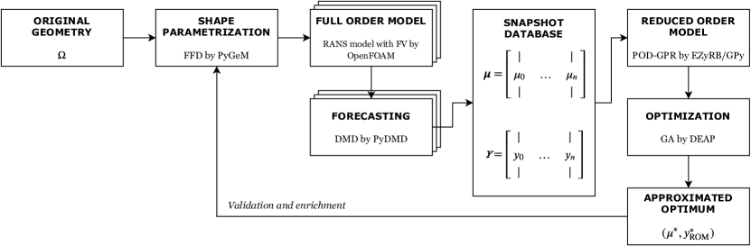
Figure 1: The flowchart of the complete computational pipeline.

This section focuses on the integration of all the components into a single pipeline capable of optimizing an input object with a generic shape $\Omega\in\mathbb{R}^{3}$. We will provide details about the methodologies stack, specifying the interfaces between methods in order to let the reader capable to understand the workflow. The proposed framework can be however, thanks to the data-driven feature, easily extended, replacing one or more tecnhniques, increasing integrability of such pipeline.

As first ingredient, we need a map $\mathcal{M}:\mathbb{R}^{3}\to\mathbb{R}^{3}$ that, depending on some numeric parameters, deforms the original domain such that $\Omega(\bm{\mu})=\mathcal{M}(\Omega,\bm{\mu})$. Dealing with complex geometries, we chose the free-form deformation (FFD) [32] to deform the original object, because of its capability to preserve continuity on the surface derivatives and to perform global deformation even with few parameters. The parameters $\bm{\mu}\in P\subset\mathbb{R}^{P}$, for this method, control the displacement of some points (along some directions) belonging to a lattice of points around the object. This motion produce a deformation in all the space embedded by the lattice. Chosen the parameter space $P$, we sample this latter $N$ times to obtain the set $\{\bm{\mu}_{i}\}_{i=1}^{N}$, and, using the FFD, the corresponding set of deformed shapes $\{\Omega(\bm{\mu}_{i})\}_{i=1}^{N}$.

The performance of all the samples have to be evaluated, using an accurate numerical solver. In this case, since the analyzed problem is related to an incompressible turbulent multiphase flow, we use the Reynolds-averaged Navier–Stokes (RANS) equations with the volume of fluid (VOF) approach to describe the mathematical model, and a finite volume (FV) discretization to numerically solve it. Such model requires, both for the complex geometry and the complexity of equations, a not-negligible amount of computational resources. Even if, as in this case, the number of these high-fidelity simulations is limited to $N$, the overall load may result too big. We can gain additional speedup exploiting the dynamic mode decomposition (DMD) [19] to predict the regime state of the simulation. In our test, the time-dependent problem shows a quasi-periodic behaviour, continuing to oscillate around the asymptotic configurations. DMD catches this kind of patterns in the temporal evolution of a system, allowing to easily make predictions with a good accuracy. We can combine the two techniques, by computing the initial temporal snapshots — aka the output of interest of such system at a certain time — with the high-fidelity model, then feeding the DMD algorithms with the latter in order to predict the regime snapshots. We define the snapshots $\mathbf{y}_{i}^{k}$ as the output of interest of the parametric domain $\Omega(\bm{\mu}_{i})$ at time $k$: the regime state $\mathbf{y}_{i}^{m+c}$ is then predicted collecting the snapshots $\{\mathbf{y}_{i}^{j}\}_{j=0}^{m}$, for $i=1,\dotsc,N$. It is important to specify that the computational grids built around the objects $\Omega(\bm{\mu}_{i})$ are not enforced to share the same topology, or the same number of degrees of freedom, but for the DMD is necessary that the grids do not change during the temporal evolution of the system. In this work we do not use the pressure and velocity fields as output of interest, but directly to the distribution of total resistance (over the surface of hull). Since the data-driven approach, this does not imply any additional complexity. Our database contains thus the discrete distribution of the total resistance for all the samples.

After this step, we obtain a set of $N$ pairs composed by the input parameters and the regime states, that is $\{(\bm{\mu}_{i},\mathbf{y}_{i}^{m+c})\}_{i=1}^{N}$. In case of output with different dimensions, we need to project the solution from the FV discretized space to the original deformed geometry $\Omega(\bm{\mu})$. Being originated by the FFD, all the geometries share the same topology. Assuming the geometry $\Omega$ is discretized in $\mathcal{N}$ degrees of freedom, the resulting new pairs are defined as $(\bm{\mu}_{i},\hat{\mathbf{y}}_{i})$, with $\bm{\mu}_{i}\in P$ and $\hat{\mathbf{y}}_{i}\in\mathbb{R}^{\mathcal{N}}$, for $i=1,\dotsc,N$.

Proper orthogonal decomposition (POD) [12] is now involved to reduce the dimensionality of the snapshots. The outputs $\hat{\mathbf{y}}_{i}\in\mathbb{R}^{\mathcal{N}}$ are projected onto the POD space, which typically has a very lower dimensions, obtaining the reduced space representation $\mathbf{c}_{i}\in\mathbb{R}^{N_{\text{POD}}}$ of the original states. The input-output pairs are now $(\bm{\mu}_{i},\mathbf{c}_{i})$ for $i=1,\dotsc,N$: assuming that a mapping $F:P\to\mathbb{R}^{N_{\text{POD}}}$ exists between input and output such that $\mathbf{c}=F(\bm{\mu})$, we can exploit the collected outputs to approximate the output itself for different parameter value using any interpolation/regression method. In this contribution, we adopt a Gaussian process regression (GPR) [27] to approximate the input-output relation with a Bayesian approach. Other examples for the POD-GPR coupling can be found in [11, 25]. Finally, the low-dimensional output is projected back to the full-order space to obtain the approximated solution. Combining the techniques, we are able to build a reduced order model based only on the system output capable to provide an approximation of the output $\mathbf{y}^{j}_{\text{ROM}}$ for untried parameters $\bm{\mu}_{j}$ in real-time. In our test, we remember we use the resistance distribution as output of interest.

The optimization procedure is then applied over the reduced order model, by computing the objective function on the state predicted using POD-GPR. Thanks to the negligible time required for the performance evaluation of a new shape, we can explore the parameter space with a genetic algorithm (GA) [16] to converge to the optimal shape. The quanity to minimize, in our numerical experiments, is the total resistance, that is nothing but the intergral of corresponding field. The objective function relies hence on the previously mentioned methods, since to compute it we need to project the POD-GPR approximation over the new shape obteined by FFD. At the end, we get the optimal parameter $\bm{\mu}^{*}$ and correspondent (approximated) output $\mathbf{y}^{*}_{\text{ROM}}$. Such parameter can be used to restart the pipeline, performing the morphing over the geometry then testing it by using the high-fidelity solver for the validation of the result. Non only: this latter simulation can be further exploited by adding it to the snapshots database, resulting in an iterative process where the approximated output is used for the reduced order model, enriching in this way the accuracy of the model itself.

Free-form deformation for shape parametrization

Free-form deformation (FFD) is a geometric tool, extensively employed in computer graphics, used to deform a rigid object based on the movement of some predefined control points. Introduced in [32], it has seen various improvements over the years. The reader can refer for example for a more recent review [2] and [20] and [30] for a coupling with ROM techniques. The main idea behind FFD is to define a regular lattice of points around the object (or part of it) and manipulate the whole embedded space by moving some of those control points. Mathematically, this is obtained by mapping the physical space enclosed by the lattice to a unit cube $D=[0,1]^{d}$ by using an invertible map $\psi:\mathbb{R}^{d}\to D$.

Inside the unit cube we define a cubic lattice of control points, with $L$,$M$ and $N$ points respectively in $x$,$y$ and $z$ directions:

$$P^{0}_{l,m,n}=\begin{pmatrix}l/L\\ m/M\\ n/N\end{pmatrix}\in D,$$ (1)

where $l=0,\dotsc,L$, $m=0,\dotsc,M$ and $n=0,\dotsc,N$ . We move these points by adding a motion $\mu_{l,m,n}$ such that:

$$P_{l,m,n}=P^{0}_{l,m,n}+\bm{\mu}_{l,m,n}.$$ (2)

The parametric map $\hat{T}:D\to D$ that performs the deformation of reference space is then defined by:

$$\hat{T}(s,t,p;\bm{\mu})=\sum_{l=0}^{L}\sum_{m=0}^{M}\sum_{n=0}^{N}b_{l}^{L}(s)b_{m}^{M}(t)b_{n}^{N}(p)P_{l,m,n},$$ (3)

where:

$$\begin{array}[]{l}b_{l}^{L}(s)=\binom{L}{l}(1-s)^{(L-l)}s^{l},\\ b_{m}^{M}(t)=\binom{M}{m}(1-t)^{(M-m)}t^{m},\\ b_{n}^{N}(p)=\binom{N}{n}(1-p)^{(N-n)}p^{n}.\\ \end{array}$$ (4)

The FFD map $T:\mathbb{R}^{3}\to\mathbb{R}^{3}$ is then composed as it follows:

$$T(\cdot;\bm{\mu})=(\psi^{-1}\circ\hat{T}\circ\psi)(\cdot;\bm{\mu}).$$ (5)

We applied the FFD algorithm directly to input object using the open source Python package called PyGeM [26].

Finite volume for high-fidelity database

We now discuss the full order model (FOM), which generates what we call the high fidelity solution. The Reynolds–averaged Navier–Stokes (RANS) equations
model the turbulent incompressible flow around the naval hull, while for the modeling of the two different phases — e.g. water and air — we adopt the volume of fluid (VOF) technique [15]. The equations governing our system are then:

$$\begin{cases}\frac{\partial\bar{u}}{\partial t}+(\bar{u}\cdot\nabla)\bar{u}+\frac{1}{\rho}\nabla\bar{p}-\nabla\cdot\nu\nabla\bar{u}-\nabla\cdot(\tilde{u}\otimes\tilde{u})=0,\\ \nabla\cdot\bar{u}=0,\\ \frac{\partial\alpha}{\partial t}+\nabla\cdot(\bar{u}\alpha)=0,\\ \end{cases}$$ (6)

where $\bar{u}$ and $\tilde{u}$ refer the mean and fluctuating velocity after the RANS decomposition, $\bar{p}$ denote the (mean) pressure, $\rho$ is the density, $\nu$ the kinematic viscosity and $\alpha$ is the discontinuous variable belonging to interval $[0,1]$ representing the fraction of the second flow in the infinitesimal volume.

The first two equations are the continuity and momentum conservation, while the third one represent the transport equation for the VOF variable $\alpha$. The Reynolds stresses tensor $\tilde{u}\otimes\tilde{u}$ can be modeled by adding additional equations in order to close the system: in this work, we use the $\text{SST}k-\omega$ turbulence model [21]. For the multiphase nature of the flow, the density $\rho$ and the kinematic viscosity $\nu$ are defined using an algebraic formula expressing them as a convex combination of the corresponding properties of the two flows:

$$\begin{array}[]{l}\rho=\alpha\rho_{1}+(1-\alpha)\rho_{2},\\ \nu=\alpha\nu_{1}+(1-\alpha)\nu_{2}.\end{array}$$ (7)

To solve such problem, we apply the finite volume (FV) approach. We adopted a $1^{st}$ order implicit Euler scheme for the temporal discretization, while for the spatial scheme we apply the linear upwind one. Regarding the software, the simulation is carried out using the C++ library OpenFOAM [23].

Dynamic mode decomposition for regime state prediction

Dynamic mode decomposition (DMD) is a data-driven ROM technique that approximates the evolution of a complex dynamical system as the combination of few features linearly evolving in time [31, 19]. The basic idea is to provide a low-dimensional approximation of the Koopman operator [18] based on few temporarily equispaced snapshots of the studied system. DMD assumes the evolution of the latter can be expressed as:

$$\mathbf{y}_{k+1}=\mathbf{A}\mathbf{y}_{k},$$ (8)

where $\mathbf{y}_{k+1}\in\mathbb{R}^{\mathcal{N}}$ and $\mathbf{y}_{k}\in\mathbb{R}^{\mathcal{N}}$ are two snapshots at the time $t=k$ and $t=k+1$, respectively, while $\mathbf{A}$ refers to a discrete linear operator. A least-square approach can be used to calculate this operator. After collecting a set of snapshots defined as $\{\mathbf{y}_{t_{0}+k\Delta t}\}_{k=0}^{M}$, we can arrange them into two matrices $\mathbf{Y}=\begin{bmatrix}\mathbf{y}_{0}&\dotsc&\mathbf{y}_{M-1}\end{bmatrix},\dot{\mathbf{Y}}=\begin{bmatrix}\mathbf{y}_{1}&\dotsc&\mathbf{y}_{M}\end{bmatrix}\in\mathbb{R}^{\mathcal{N}\times M}$ such that the correspondent columns of the two matrices represent two sequential snapshots.

We can now minimizing the error $\|\mathbf{A}\mathbf{Y}-\dot{\mathbf{Y}}\|_{F}$ by the following matrix multiplication $\mathbf{A}=\dot{\mathbf{Y}}\mathbf{Y}^{\dagger}$, where the symbol ^† indicates the Moore-Penrose pseudoinverse. While we can already use the operator $\mathbf{A}$ to analyze the system, in practice because of its considerable dimension and the difficulties that would arise in order to obtain it numerically. DMD uses then the singular value decomposition (SVD) to compute the reduced space onto which projecting the operator. Formally

$$\mathbf{Y=U\Sigma V}^{T},$$ (9)

where $\mathbf{U}\in\mathbb{R}^{\mathcal{N}\times M}$, $\mathbf{\Sigma}\in\mathbb{R}^{M\times M}$ and $\mathbf{V}\in\mathbb{R}^{M\times M}$. The left singular vectors (the columns of $\mathbf{U}$) span the optimal low-dimensional space, allowing us to project the operator $\mathbf{A}$ onto it:

$$\mathbf{\tilde{A}=U}^{T}\mathbf{AU=U}^{T}\mathbf{\dot{Y}V\Sigma}^{-1}$$ (10)

to compute the reduced operator. The interesting feature is that the eigenvalues of $\mathbf{\tilde{A}}$ are equal to the non-zero ones of the high dimensional operator $\mathbf{A}$, and also the eigenvectors of the two operators are related each other [36]. In particular:

$$\mathbf{\Phi=\dot{Y}V\Sigma}^{-1}\mathbf{W},$$ (11)

where $\Phi$ is the matrix containing the $\mathbf{A}$ eigenvectors, the so-called DMD modes, and $\mathbf{W}$ is the matrix of $\tilde{\mathbf{A}}$ eigenvectors. Defining $\mathbf{\Lambda}$ as the diagonal matrix of eigenvalues, we have:

$$\mathbf{Y}\approx\mathbf{A}\mathbf{X}=\mathbf{\Phi}\mathbf{\Lambda}\mathbf{\Phi}^{\dagger}\mathbf{X}$$ (12)

that implies that any snapshots can be approximated computing $\mathbf{y}_{k}=\mathbf{\Phi}\mathbf{\Lambda}^{k}\mathbf{\Phi}^{\dagger}\mathbf{y}_{0}$.

We apply the DMD on the snapshots coming from the full-order model (discussed in subsection 2.2) in order to perform fewer temporal iterations using the high-fidelity solver, and predict the output we are interested to analyze in order to gain an additional considerable speedup. The results are obtained using PyDMD [7], a Python package that implements the most common version of DMD.

Reduced order model exploiting proper orthogonal decomposition

Reduced basis (RB) is a ROM method that approximates the solution manifold of a parametric problem using a low number of basis functions that form what we call the reduced basis [28, 12]. In this community, proper orthogonal decomposition (POD) is a widespread technique [3, 33] since its capability to provide orthogonal basis that have an energetically hierarchy. While a possible approach for turbulent flows involving projection-based ROM is available in [13], we prefer the data-driven approach for the higher integrability in many industrial workflows. POD needs as input a matrix containing samples of the solution manifold. We define $\mathcal{N}$ the number of degrees of freedom of our numerical model and $\mathbf{y}\in\mathbb{R}^{\mathcal{N}}$ its solution for a generic parameter $\bm{\mu}$. Thus, the snapshots matrix $\mathbf{Y}\in\mathbb{R}^{\mathcal{N}\times n}$ is defined as:

$$\mathbf{Y}=\left[\begin{array}[]{cccc}\vrule&\vrule&&\vrule\\ \mathbf{y}_{1}&\mathbf{y}_{2}&\ldots&\mathbf{y}_{n}\\ \vrule&\vrule&&\vrule\end{array}\right].$$ (13)

The POD basis is defined as basis that maximizes the similarity (as measured by the square of the scalar product) between the snapshots matrix and its elements, under the constraint of orthonormality. Formally, the POD basis $\{\psi_{i}\}_{i=0}^{l}$ of dimension $l$ is defined as:

$$\max_{\psi_{1},\dotsc\psi_{l}}\sum_{i=1}^{l}\sum_{j=1}^{n}|\langle\mathbf{y}_{j},\psi_{i}\rangle_{\mathbb{R}^{\mathcal{N}}}|^{2}$$ (14)

such that $\langle\tilde{\psi_{i}},\tilde{\psi_{i}}\rangle_{\mathbb{R}^{\mathcal{N}}}=\delta_{i,j}$, for $1\leq i,j\leq l$. Singular value decomposition (SVD) is a method that computes the POD basis [37] by decomposing the snapshots matrix:

$$\mathbf{Y}=\mathbf{U}\mathbf{\Sigma}\mathbf{V}^{*},$$ (15)

where matrices $\mathbf{U}\in\mathbb{R}^{\mathcal{N}\times n}$ and $\mathbf{V}\in\mathbb{R}^{n\times n}$ are unitary while $\mathbf{\Sigma}\in\mathbb{R}^{n\times n}$ is diagonal. In particular, the columns of $\mathbf{U}$ are POD basis. We project the original snapshots onto the POD space to have a low-dimensional representation. In matrix form:

$$\mathbf{C}=\mathbf{U}^{T}\mathbf{Y},\quad\mathbf{c}\in\mathbb{R}^{n\times n}.$$ (16)

The columns of $\mathbf{C}$ are the modal coefficients $\mathbf{c}_{i}\in\mathbb{R}^{n}$.

We can now exploit this reduced space in order to build a probabilistic response surface using the Gaussian process regression (GPR) [27]. In particular, assuming there is a natural relation $F:P\to\mathbb{R}^{n}$ between our geometric parameters $\bm{\mu}$ and the low-dimensional output $\mathbf{c}$ such that $\mathbf{c}=F(\bm{\mu})$, we try to approximate it with a multivariate Gaussian distribution. We define:

$$f(\bm{\mu})\sim\text{GP}(\mathcal{M}(\bm{\mu}),\mathcal{K}(\bm{\mu},\bm{\mu})),$$ (17)

where $\mathcal{M}$ refers to the mean of the distribution and $\mathcal{K}$ to its covariance. There are many possible choices for the covariance function $\mathcal{K}:P\times P\to\mathbb{R}$, in our case we use the the squared exponential one defined as $\mathcal{K}_{SE}(\bm{\mu}_{i},\bm{\mu}_{j})=\sigma^{2}\exp(-\frac{1}{2}\|\bm{\mu}_{i}-\bm{\mu}_{j}\|^{2})$. The prior joint Gaussian distribution for the outputs $\mathbf{c}$ results then

$$\mathbf{c}|\mathbf{\bm{\mu}}\sim~{}\mathcal{N}(0,\mathcal{K}(\bm{\mu},\bm{\mu})).$$ (18)

For sake of simplicity we assume that the GP has mean equal to zero: the entire process results defined only by the covariance function. In order to specify the GP for our dataset, we need to maximize the marginal likelihood varying the hyper-parameters of the covariance function, in this case only the $\sigma$. Once obtained the output distribution, we can just sample it at the test parameters to predict the output — which, we remember, is the low-dimensional snapshot — by exploiting the joint distribution:

$$\bar{\mathbf{c}}|\bar{\bm{\mu}},\bm{\mu},\mathbf{c}\sim\mathcal{N}(\mathbf{m},\mathbf{C})$$ (19)

with

$$\begin{array}[]{ll}\mathbf{m}&=\mathcal{K}(\bar{\bm{\mu}},\bm{\mu})\mathcal{K}(\bm{\mu},\bm{\mu})^{-1}\mathbf{c},\\ \mathbf{C}&=\mathcal{K}(\bar{\bm{\mu}},\bar{\bm{\mu}})-\mathcal{K}(\bar{\bm{\mu}},\bm{\mu})\mathcal{K}(\bm{\mu},\bm{\mu})^{-1}\mathcal{K}(\bm{\mu},\bar{\bm{\mu}}),\end{array}$$ (20)

where $\bm{\mu}$ and $\bar{\bm{\mu}}$ refer to the input parameters and the test parameters, and where $\mathbf{c}$ and $\bar{\mathbf{c}}$ are the corresponding train and test output.

We compute the modal coefficients of all (untested) new parameters. To approximate the high-dimensional snapshots we need just to back map the modal coefficients to the original space. In matricial form:

$$\bar{\mathbf{y}}=\mathbf{U}\bar{\mathbf{c}}$$ (21)

An additional gain of such method is the complete division between two computational phases often called offline and online steps We can easily note that, to collect the input snapshots, we initially need to compute several snapshots using the chosen high-fidelity model. This is the most expensive part, and usually is carried out on powerful machines. This offline step is fortunately independent from the online one, where actually the snapshots are combined to span the reduced space and approximate the new reduced snapshots. Since this latter can be easily performed on standard laptops, the computational splitting in two steps allows also to efficiently exploit all different resources.

For the implementation, we developed and released this verion of data-driven POD in the numerical open source package EZyRB [6], exploiting the library GPy [10] for the GPR step.

Genetic algorithm for global optimization

Genetic algorithms (GA) denote in literature the family of computational methods that are inspired by Darwin’s theory of evolution. In an optimization context, emulating the natural behaviour of living beings, this methodology gained popularity due to its easy application and the capability to not get blocked in local minima. The algorithm was initially proposed by Holland in [16, 17, 1] and it is based on few fundamental steps: selection, mutation and mate. We consider any sample of the parameter domain as an individual $\bm{\mu}_{i}\in P\subset\mathbb{R}^{P}$ with $P$ chromosomes. The fitness of the individuals is quantify by a scalar objective function $f:P\to\mathbb{R}$. We define the initial population $\mathbf{M}^{0}=\{\bm{\mu}_{i}\}_{i=1}^{N_{0}}$ composed by $N_{0}$ individuals that are randomly created within the parameter space. The corresponding fitnesses are compute and the evolutive process of individuals starts.

The first step is the selection of the best individuals in the population. Intuitively, the basic approach results chosing the $N$ individuals that have the highest fitnesses, but for large population, or simply to reinforce the stocastich component of the method, a propabilistic selection can be performed. The selected individuals are often refered as the offspring that will breed the future generation.

We are now ready to reproduce the random evolution of such individuals. This is done in the mutation and mate steps. In the mutation, chromosomes of the individuals can change, partially or entirelly, in order to create the new individuals. Several approaches are available for the mutation, but usually they are based to a mutation probability to reproduce the aleatory nature of evolution. In the mate step, individuals are coupled into pairs and, still randomly, the chromosomes of the parent individuals are combined to originate the two children. In particular, the mate step emulates the reproduction step, and for this reason can be usually called also cross-over.

The population is now composed by the new (mated and mutated) individuals. Iterating this process, the population will converge toward the optimal individual, but depending on the shape of fitness function it may requires many generations to converge.

For the numerical experiments, we use the GA implementation provided by the DEAP [9] package, an open source library for evolutionary algorithms.

3 Numerical results: a cruise ship shape optimization

In this section, we will present the results obtained by applying the described computational pipeline to optimize the shape of a cruise ship. We maintain the same structure of the previous section, discussing the intermediate results for any mentioned technique.

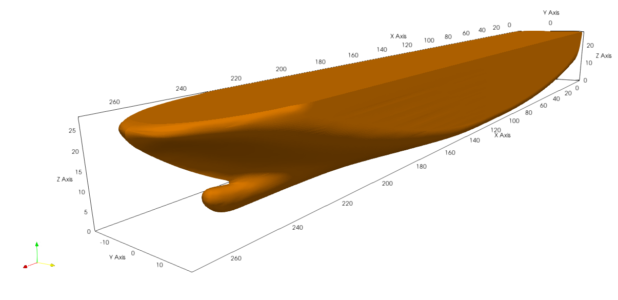
Figure 2: The undeformed hull.

Free-form deformation

We set the domain $D$, aka the space enclosed by the lattice of FFD control points, in order to deform only the immersed part of the hull, in the proximity of the bow. The lattice is illustrated in Figure 3, and we can see that it is positioned, in $x$ direction, on sections $10,12,14,16,18,20$ and 22. For $z$ direction, the points are displaced around the waterline, while along $y$ axis the points are positioned for the entire width of the ship. In total, $539$ FFD points are used.

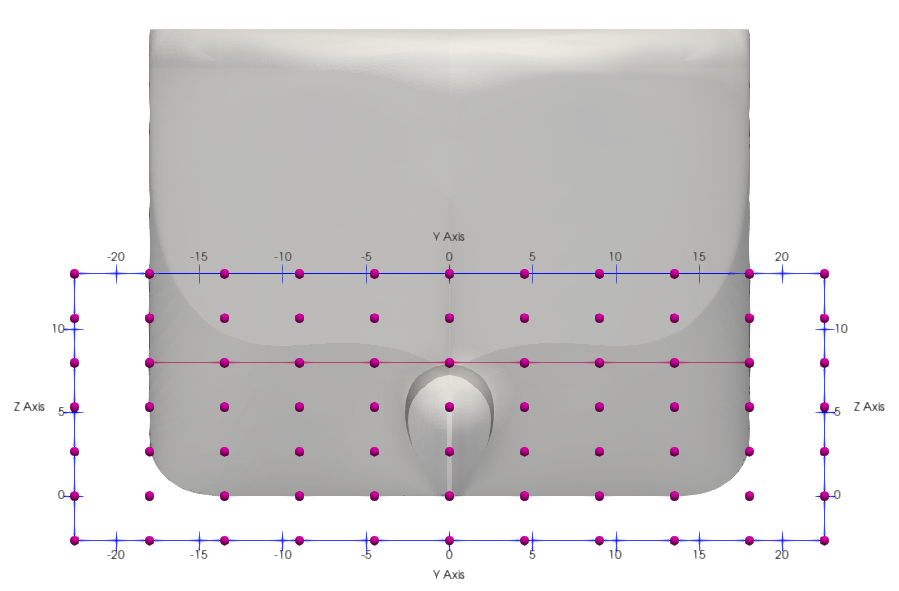
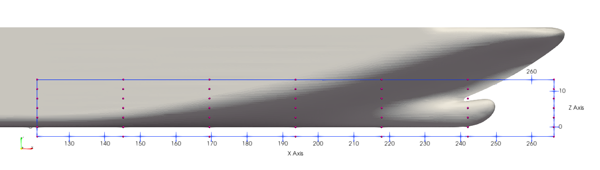
Figure 3: $x$- and $y$-normal view of the set $D$ (in blue) and the lattice of points $P^{0}_{l,m,n}$ (in red) over the undeformed hull.

Concerning the motion of such points only part of the points in the lattice are displaced: we use $6$ parameters to control the movements along $x$ (the first three parameters) and along $y$. An example of this motion is sketched in Figure 4, where red arrows refers to control points movements. The layers corresponding to sections $10,12,20$ and $22$ remain fixed, together with the two upper and lower layers, the two far left and the two far-right layers and, finally, the layer over the longitudinal symmetry plane. Except for this last one, that is kept fixed to maintain symmetry, the other layers are kept fixed in order to achieve the continuity and smoothness of the shapes, required especially in the $x$ direction where the deformation must link in a smooth way to the rest of the boat.

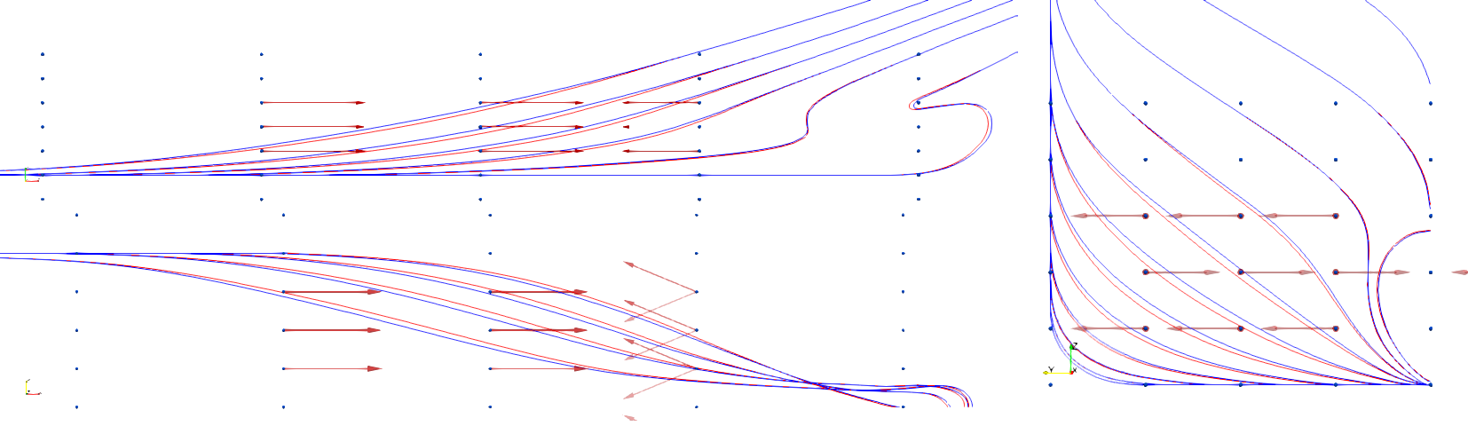
Figure 4: Example of shape morphing with $\bm{\mu}~{}=~{}[0.08,0.08,-0.06,0.08,-0.08,0.08]$

The parameter range have been chosen in order to avoid a high decrease of the hull volume and, at the same time, explores a large variety of new shapes. In details, we have a tolerance of the $1\permil$ for the volume constraint. With a trial and error approach we define the parameter ranges, obtaining a parameter space that is $P=[-0.08,0.08]^{6}$ (the dimension of such space is the number of parameters, $6$ in this test). We underline that the parameters refer to the motion normalized for the $D$ length along the corresponding direction.

We create a set of $100$ samples taking with uniform distribution on the parametric space. These are the input parameters of the high-fidelity database required for ROM.

Finite volume discretization

We simulate the flow pasting around the ship using the FV method, computing for each deformed object the distribution of the total resistance over the hull. The simulations are run on model scale ($1:25$). The computational grid (defined in $[-39,24]\times[-29,0]\times[-24,6]$) is built from scratch around all the deformed hulls, enforcing the mesh quality. The computational grid counts $\approx$1.5\text{\times}{10}^{6}$$ cells. To the VOF model, we need an extra refinement around the waterline in order to avoid a diffusive behavior of the fraction variable $\alpha$, which is discontinuous. A region of the computation grid is reported in Figure 5 for demonstrative purpose.

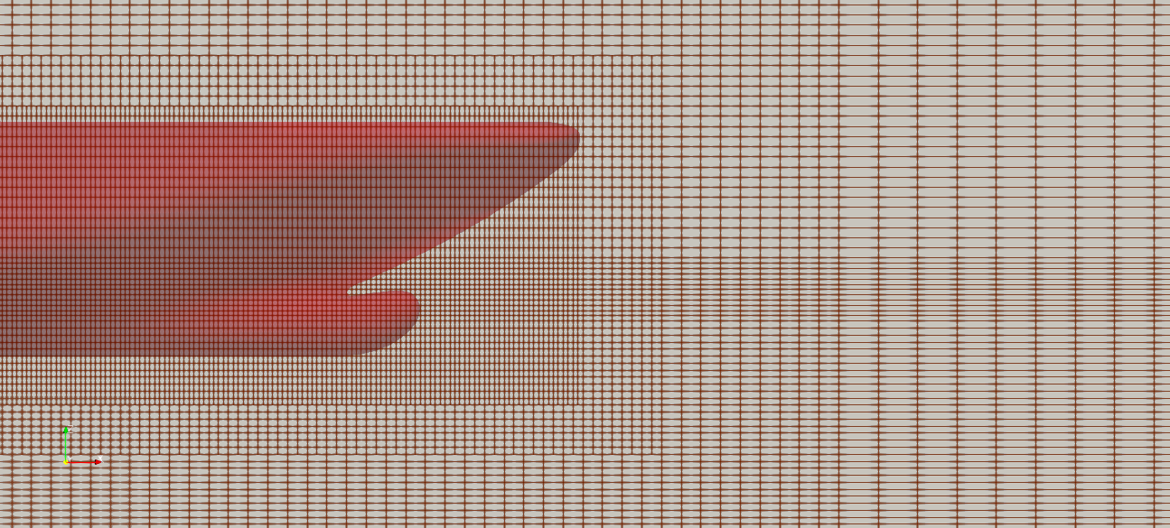
Figure 5: The refined computational grid

The numerical schemes adopted are mentioned in subsection 2.2, and we report in Table 1 the main physical quantities we fix in our setting. The Reynolds number is near to $2\text{\times}{10}^{7}$.

Table 1: Summary of the numerical variable for VOF-RANS model

inlet velocity $u$	$2.263\,36\text{\,}\mathrm{m}\text{\,}{\mathrm{s}}^{-1}$
water density $\rho_{W}$	$1.09\text{\times}{10}^{-6}\text{\,}\mathrm{m}^{2}\mathrm{/}\mathrm{s}$
air density $\rho_{A}$	$1.09\text{\times}{10}^{-5}\text{\,}\mathrm{m}^{2}\mathrm{/}\mathrm{s}$
water kinematic viscosity $\nu_{W}$	$998.8\text{\,}\mathrm{k}\mathrm{g}\mathrm{/}\mathrm{m}^{3}$
air kinematic viscosity $\nu_{A}$	$1\text{\,}\mathrm{k}\mathrm{g}\mathrm{/}\mathrm{m}^{3}$
dissipation rate $\omega$	$70.497\,21\text{\,}\mathrm{s}^{-1}$
turbulent kinetic energy $k$	$7.6841\text{\times}{10}^{-4}\text{\,}\mathrm{m}^{2}\mathrm{/}\mathrm{s}^{2}$

The integration in time is carried out for $t\in[0,40]~{}$\mathrm{s}$$, with an initial step of $\Delta t=$1\text{\times}{10}^{-3}\text{\,}\mathrm{s}$$ and an adjustable time-stepping governed by the Courant number (we impose it to be lower than $5$). We clarify that, even if the time stepping is not fixed, we save the equispaced temporal snapshots of the system in order to feed the DMD algorithm. In this work, we are interested to the total resistance of the ship: after computing the pressure, velocity and fraction variable unknowns (from the VOF-RANS model), we can exploit them in order to calculate the resistance distribution (both the viscous and the friction terms) over the hull surface. Regarding the computing time, on a parallel architecture with $40$ processes, the simulation lasts approximately $8$ hours.

Dynamic mode decomposition

We applied DMD on the results of the FOM. It is important to specify that we fit a DMD model for each geometric deformation, as a sort of post-processing on the output. We train the model using the snapshots $\{\mathbf{y}_{i}\}_{i=0}^{40}$ for $i=t_{\text{dmd}}^{0}+i\Delta t_{\text{dmd}}$, with $t_{\text{dmd}}^{0}=$20\text{\,}\mathrm{s}$,\Delta t_{\text{dmd}}=$0.5\text{\,}\mathrm{s}$$. The first $20\text{\,}\mathrm{s}$ of the simulation are discarded since they are not particularly meaningful for the boundary conditions propagation.

Figure 6: First 5 DMD eigenvalues for a single simulation.

In this contribution, we analyze the DMD operator from a spectral perspectives. Figure 6 reports in fact the eigenvalues (computed for a single simulation) after projecting the output onto a POD space of dimension $5$. The position of eigenvalues in the complex plane provide information about the dynamics of all the DMD modes. In particular, the imaginary part is related to frequency, while the distance between them and the unit circle is related to the growth-rate. We can neglect the dumped modes (the two eigenvalues inside the circle) since their contribution is useless for future dynamics and focus on the remaining ones: two modes present a stable oscillatory trend, that actually catch the asymptotic oscillations of the FOM, and the last one ($1+0i$) is practically constant. We isolate the contribution of only this latter mode, assuming it represents the regime state to which the FOM converges, using it as final output. In our setting, having built the computational grid for all the deformed ships from scratch, we need as last step to project the resistance distribution over the initial geometry $\Omega(\bm{\mu})$, in order to ensure same dimensionality for all the outputs. In our case we use a closest neighbors interpolation. Thanks to the application of DMD, we can perform fewer time iterations in the full-order model: in this case we can reduce the simulated seconds from $60$ to $40$, approximating the regime state with DMD. This of course implies a reduction of $\nicefrac{{1}}{{3}}$ of the overall time required to run all the simulations.

Proper orthogonal decomposition with Gaussian process regression

We exploit the collected database in order to build a kind of probabilistic response surface to predict the resistance of new shapes. We remember the starting set is composed by $100$ input-output pairs $\{(\bm{\mu}_{i},\mathbf{y}_{i})\}_{i=1}^{100}$, where $\bm{\mu}$ is the geometrical parameters provided to FFD and $\mathbf{y}$ is the resistance distribution over the deformed hull. Of the entire set, we use the $80\%$ for train the POD-GPR framework and exploit the remaining pairs to test our method. Firstly we applied the POD on the snapshots matrix to reduce the dimension of the output.

Figure 7: Values of $\frac{\sigma_{i}}{\sigma_{0}}$ for the first 40 singular values, ordered from the highest to the lowest value.

In this case the singular values extracted are reported in Figure 7 from an energetic perspective. The decay-rate is not very steep, probably due to the discontinuous component for the VOF variable $\alpha$, which is directly involved in the resistance computation.

Figure 8: Sensitivity analysis on the accuracy of POD-GPR method varying the number of POD modes used. The number of snapshots is fixed to $80$.

Despite this, the POD allows to remarkably reduce the dimension of the output, simplifying the next phase. We exploit the computed modal coefficient in order to optimize the GP, then query for the new parametric solutions. To measure the accuracy, we propose in Figure 8 and Figure 9 two different sensitivity analysis varying the number of POD modes used to span the reduced space and the number of snapshots to train the method, respectively. For sake of completeness, we compare the results with similar data-driven methodologies that involve, instead the GPR, other interpolation techniques for modal coefficient approximation, as the linear interpolation one or the radial basis function (RBF) one. We propose here the simplest RBF interpolation, but we make the reader aware that better results can be achieved tuning the smoothness of RBF, producing a non-interpolating RBF method. For more details we refer [24]. The error refers to the mean relative error computed on the test dataset (of dimension $20$), using the resistance distribution coming from DMD as truth solution. The GPR method is able to reach the minimum error respect to the other interpolation, resulting in a relative error near to $5\%$ adopting $20$ modes, but reducing its accuracy increasing the number of modes. This trend is shown also by RBF error, that after an initial decreasing, becomes very large for many modes.

Figure 9: Sensitivity analysis on the accuracy of POD-GPR method varying the number of snapshots. The number of POD modes is fixed to $20$.

Varying the number of snapshots (Figure 9), the difference between RBF and GPR is even more evident. While the RBF reaches an error slightly less than the $8\%$, the GPR is able to stay beyond the $6\%$ with $80$ snapshots. We note that we get the highest difference between the methods using few snapshots: the GPR shows higher accuracy even with few samples and a pretty constant trend for database with greater dimension.

Figure 10: Value of total resistance over the bulbous bow for the FOM (on the left) and for the ROM (on the right).

Finally, we conclude with a graphical visualization of the resistance distribution on (a limited region of) the hull in Figure 10, comparing the ROM approximation with the FOM validation. Even if the difference is notable, the reduced model can express the main physics behaviour of the original model. Regarding the computational cost reduction, the reduced model can approximate the parametric solution only sampling an already defined distribution, and even on a personal laptop it takes no more than few seconds, whereas the FV solver takes $8$ hours, resulting in a very huge speedup.

Genetic algorithm

The goal of the entire pipeline is the minimization of the total resistance (only in the direction of the flow). To ensure feasibility of the deformed shape from the engineering viewpoint, we add a penalization on the hulls whose volume is lower that $999\permil$ of the original hull. In other words, we penalize the configurations that lead a volume decrease greater than $\nicefrac{{1}}{{1000}}$ with respect to the original volume. Our optimization problem reads:

$$\underset{\bm{\mu}}{\text{min}}\left\{\begin{aligned} &\smallint_{\Omega(\bm{\mu})}\tau_{x}\rho-pn_{x}\quad&\text{if}\smallint_{\Omega(\bm{\mu})}\rho gh&\geq 0.999\smallint_{\Omega}\rho gh\\ &\infty&\text{otherwise}&\\ \end{aligned}\right.$$ (22)

where $\tau_{x}$ is the $x$ component of the (viscous and turbulent) tangential stresses, $\rho$ is the density of the fluid (computed according to the VOF model), $p$ is the pressure, $n_{x}$ is the $x$ component of the normal to the surface, $g$ is the gravity acceleration and $h$ is the distance between the surface and the waterline ($\smallint_{\Omega}\rho gh$ results the volume of the immersed hull using an hydrostatic approach). To compute the objective function for a generic parameters, we need to perform the FFD morphing then project the POD-GPR solutions over the deformed ship, in order to numerically compute such integral. We clarify that with the reduced order model returns the distribution of viscous and pressure forces over the hull, that is $\tau\rho-p$ in $\Omega(\bm{\mu})$. As already mentioned, these methods have a negligible computational cost, allowing us to optimize the shape in a very efficient manner. Despite its easiness of application, GA requires a good tuning of the hyper-parameters to result successful. In this work, we applied the one point crossover [8] for the mate procedure, while for the mutation a Gaussian mutation [14] with $\sigma=0.1$ has been involved. We set the mate and mutation probability to $0.8$ and $0.2$, respectively. Moreover, we use an initial population dimension $N_{0}=200$, reducing it to $N=30$ during the evolution. The stopping criteria in this case is the number of generations, which is set to $15$. Robustness of this setting is proved in Figure 11, where $15$ different runs have been run and, for each run, the optimal shape is plotted both in terms of resistance and volume.

Figure 11: Optimal shapes produced by $15$ different application of GA, in terms of resistance and volume as percentage respect to the original ship.

We can note in fact that all the runs have converged to the same fitness, despite the stochastic component of the method itself, ensuring that the hyper-parameters are set to fully explore the parameter space (and then globally converge to the optimal point). The penalization we impose avoids the creation of unfeasible deformations: the optimum of all the runs show a slight decreased volume, but within the initial tolerance, while the resistance results decreased by more than the $4\%$.

We specify that this is the optimum for the reduced model. In order to obtain an accurate value, the optimal parameter can be plug in the pipeline and the optimal shape is then validated using the full-order FV method. Additionally, this latter can be insert in the snapshots database and used to enrich the precision of the POD-GPR model. In our case, after the validation, the gain in term of resistance is lower with respect to the ROM approximation, but reaching the $3.3\%$ it results in a very good outcome in the engineering context.

4 Conclusion and future perspectives

In this work, we propose a complete computational framework for shape optimization problems. To overcome the computational barrier, the dynamic mode decomposition (DMD) and the proper orthogonal decomposition with Gaussian process regression (POD-GPR) are involved. This pipeline aims at reducing the number of high-fidelity simulation needed to converge to the optimal shape, making its application very useful in all the context where the performance evaluation of the studied object results computationally expensive. We applied such framework to an industrial shape optimization problem, minimizing the total resistance of a cruise ship advancing in calm water. Exploitation of ROM techniques drastically reduces the overall time, and even if the accuracy of the reduced model is decreased (with respect to the full-order one) the final outcome presents a remarkable reduction of the resistance ($3.3\%$).

Future developments regarding this integrated methodology may interest the extension to constraint optimization problems, the involvement of machine learning techniques in the optimization procedure, or a greedy approach that enriches the reduced order model by adding iteratively the approximated optimal shape.

References

- [1] T. Back. Evolutionary algorithms in theory and practice: evolution strategies, evolutionary programming, genetic algorithms. Oxford University Press, 1996.
- [2] F. Ballarin, A. Manzoni, G. Rozza, and S. Salsa. Shape optimization by free-form deformation: Existence results and numerical solution for Stokes flows. Journal of Scientific Computing, 60(3):537–563, 2014.
- [3] F. Ballarin, G. Rozza, and Y. Maday. chapter Reduced-order semi-implicit schemes for fluid-structure interaction problems, pages 149–167. Springer International Publishing, 2017.
- [4] N. Demo, M. Tezzele, G. Gustin, G. Lavini, and G. Rozza. Shape optimization by means of proper orthogonal decomposition and dynamic mode decomposition. In Technology and Science for the Ships of the Future: Proceedings of NAV 2018: 19th International Conference on Ship & Maritime Research, pages 212–219. IOS Press, 2018.
- [5] N. Demo, M. Tezzele, A. Mola, and G. Rozza. A complete data-driven framework for the efficient solution of parametric shape design and optimisation in naval engineering problems. In VIII International Conference on Computational Methods in Marine Engineering, 2019.
- [6] N. Demo, M. Tezzele, and G. Rozza. EZyRB: Easy Reduced Basis method. The Journal of Open Source Software, 3(24):661, 2018.
- [7] N. Demo, M. Tezzele, and G. Rozza. PyDMD: Python Dynamic Mode Decomposition. The Journal of Open Source Software, 3(22):530, 2018.
- [8] L. J. Eshelman and J. D. Schaffer. Real-coded genetic algorithms and interval-schemata. In Foundations of genetic algorithms, volume 2, pages 187–202. Elsevier, 1993.
- [9] F.-A. Fortin, F.-M. De Rainville, M.-A. Gardner, M. Parizeau, and C. Gagné. DEAP: Evolutionary algorithms made easy. Journal of Machine Learning Research, 13:2171–2175, jul 2012.
- [10] GPy. GPy: A Gaussian process framework in Python. http://github.com/SheffieldML/GPy, since 2012.
- [11] M. Guo and J. S. Hesthaven. Reduced order modeling for nonlinear structural analysis using Gaussian process regression. Computer Methods in Applied Mechanics and Engineering, 341:807–826, 2018.
- [12] J. S. Hesthaven, G. Rozza, and B. Stamm. Certified Reduced Basis Methods for Parametrized Partial Differential Equations. Springer Briefs in Mathematics. Springer, Switzerland, 1 edition, 2015.
- [13] S. Hijazi, G. Stabile, A. Mola, and G. Rozza. Data-Driven POD-Galerkin Reduced Order Model for Turbulent Flows. Submitted, 2019.
- [14] R. Hinterding. Gaussian mutation and self-adaption for numeric genetic algorithms. In Proceedings of 1995 IEEE International Conference on Evolutionary Computation, volume 1, page 384. IEEE, 1995.
- [15] C. Hirt and B. Nichols. Volume of fluid (vof) method for the dynamics of free boundaries. J. Comput. Phys., 39:201–225, 1 1981.
- [16] J. H. Holland. Genetic algorithms and the optimal allocation of trials. SIAM Journal on Computing, 2(2):88–105, 1973.
- [17] J. H. Holland. Adaptation in natural and artificial systems: an introductory analysis with applications to biology, control, and artificial intelligence. MIT press, 1992.
- [18] B. O. Koopman. Hamiltonian systems and transformation in Hilbert space. Proceedings of the National Academy of Sciences of the United States of America, 17(5):315, 1931.
- [19] J. N. Kutz, S. L. Brunton, B. W. Brunton, and J. L. Proctor. Dynamic Mode Decomposition: Data-Driven Modeling of Complex Systems. SIAM, 2016.
- [20] T. Lassila and G. Rozza. Parametric free-form shape design with PDE models and reduced basis method. Computer Methods in Applied Mechanics and Engineering, 199(23-24):1583–1592, 2010.
- [21] F. Menter. Zonal two equation kw turbulence models for aerodynamic flows. In 23rd fluid dynamics, plasmadynamics, and lasers conference, page 2906, 1993.
- [22] A. Mola, M. Tezzele, M. Gadalla, F. Valdenazzi, D. Grassi, R. Padovan, and G. Rozza. Efficient reduction in shape parameter space dimension for ship propeller blade design. In Proceedings of MARINE 2019: VIII International Conference on Computational Methods in Marine Engineering, pages 201–212, 2019.
- [23] OpenCFD. OpenFOAM - The Open Source CFD Toolbox - User’s Guide. OpenCFD Ltd., United Kingdom, 6 edition, 7 2018.
- [24] G. Ortali. A Data-Driven Reduced Order Optimization Approach for Cruise Ship Design. Master’s thesis, Politecnico di Torino, 2019.
- [25] G. Ortali, N. Demo, G. Rozza, and C. Canuto. Gaussian process approach within a data-driven POD framework for fluid dynamics engineering problems. Submitted, 2020.
- [26] PyGEM. PyGEM: Python geometrical morphing. Available at https://github.com/mathLab/PyGeM.
- [27] J. Quiñonero-Candela and C. E. Rasmussen. A unifying view of sparse approximate gaussian process regression. Journal of Machine Learning Research, 6(Dec):1939–1959, 2005.
- [28] G. Rozza, M. W. Hess, G. Stabile, M. Tezzele, and F. Ballarin. Basic Ideas and Tools for Projection-Based Reduced Order Methods: Preliminaries and Warming-Up. In P. Benner, S. Grivet-Talocia, A. Quarteroni, G. Rozza, W. H. A. Schilders, and L. M. Silveira, editors, Handbook on Model Order Reduction, volume 1, chapter 1. De Gruyter, 2019.
- [29] G. Rozza, M. H. Malik, N. Demo, M. Tezzele, M. Girfoglio, G. Stabile, and A. Mola. Advances in Reduced Order Methods for Parametric Industrial Problems in Computational Fluid Dynamics. In R. Owen, R. de Borst, J. Reese, and P. Chris, editors, ECCOMAS ECFD 7 - Proceedings of 6th European Conference on Computational Mechanics (ECCM 6) and 7th European Conference on Computational Fluid Dynamics (ECFD 7), pages 59–76, Glasgow, UK, 2018.
- [30] F. Salmoiraghi, A. Scardigli, H. Telib, and G. Rozza. Free-form deformation, mesh morphing and reduced-order methods: enablers for efficient aerodynamic shape optimisation. International Journal of Computational Fluid Dynamics, 32(4-5):233–247, 2018.
- [31] P. J. Schmid. Dynamic mode decomposition of numerical and experimental data. Journal of fluid mechanics, 656:5–28, 2010.
- [32] T. W. Sederberg and S. R. Parry. Free-form deformation of solid geometric models. In IN: SIGGRAPH, 1986. PROCEEDINGS, pages 151–160, 1986.
- [33] G. Stabile and G. Rozza. Finite volume POD-Galerkin stabilised reduced order methods for the parametrised incompressible Navier–Stokes equations. Computers & Fluids, 173:273–284, Sept. 2018.
- [34] M. Tezzele, N. Demo, and G. Rozza. Shape optimization through proper orthogonal decomposition with interpolation and dynamic mode decomposition enhanced by active subspaces. In Proceedings of MARINE 2019: VIII International Conference on Computational Methods in Marine Engineering, pages 122–133, 2019.
- [35] M. Tezzele, N. Demo, G. Stabile, A. Mola, and G. Rozza. Enhancing CFD predictions in shape design problems by model and parameter space reduction. arXiv preprint arXiv:2001.05237, Submitted, 2019.
- [36] J. Tu, C. Rowley, D. Luchtenburg, S. Brunton, and N. Kutz. On dynamic mode decomposition: Theory and applications. Journal of Computational Dynamics, 1(2):391–421, 2014.
- [37] S. Volkwein. Proper orthogonal decomposition: Theory and reduced-order modelling. Lecture Notes, University of Konstanz, 01 2012.