Influence of parallel computing strategies of iterative imputation of missing data: a case study on missForest

Abstract

Machine learning iterative imputation methods have been well accepted by researchers for imputing missing data, but they can be time-consuming when handling large datasets. To overcome this drawback, parallel computing strategies have been proposed but their impact on imputation results and subsequent statistical analyses are relatively unknown. This study examines the two parallel strategies (variable-wise distributed computation and model-wise distributed computation) implemented in the random-forest imputation method, missForest. Results from the simulation experiments showed that the two parallel strategies can influence both the imputation process and the final imputation results differently. Specifically, even though both strategies produced similar normalized root mean squared prediction errors, the variable-wise distributed strategy led to additional biases when estimating the mean and inter-correlation of the covariates and their regression coefficients.

1 Introduction

Missing data are common in most research, and various kinds of imputation methods have been proposed for handling missing data problems. Stekhoven and Buhlmann (Stekhoven and Buhlmann 2012) proposed the missForest algorithm based on a random forest (RF) machine learning method (Liaw and Wiener 2002), and it has been used in different studies and benchmarked against other imputation methods (Ramosaj and Pauly 2019; Shah et al. 2014; Tang and Ishwaran 2017; Waljee et al. 2013).

Moreover, new imputation methods have been proposed based on the original missForest algorithm (Mayer 2019). MissForest has been shown to have superior predictive accuracy under certain circumstances, but it necessitates the building of a large number (default is 100) of trees during the imputation process for a single variable per iteration and usually several iterations are required. Likewise, missForest can be computationally intensive and time-consuming for large datasets, thereby limiting its usability. To boost performance, two parallel computing strategies (referred to as “forests” and “variables” in the software package) suitable for “long” and “wide” datasets, respectively (Stekhoven 2013), were implemented in missForest with the release of version 1.4. However, there has not been any published evaluation of their difference on predictive accuracy and subsequent impact on statistical analyses. The implicit assumption is that these two strategies are equally valid and will lead to similar results.

This study uses simulation experiments to address the differences between these two parallel computation strategies of missForest. Computational efficiency can be critical for handling large datasets; thus, this study’s results can be of use to both data analytics practitioners and methodologists for imputation methods.

2 Methods

2.1 MissForest algorithm

In missForest, the variables containing missing values are initialized for imputation by replacing the missing cells by corresponding mean values (for continuous variables), or by the most frequent category (for categorical variables). A variable under imputation is then divided into two distinct parts: the observed part that contains no missing values, and the missing part that serves as the prediction set. A random forest is fitted using the observed part as response and the corresponding values of the other variables as predictors, and the missing part is replaced with the predicted values from the random forest. The algorithm then proceeds to the next variable to be imputed, and the iteration stops when the difference between the current and previously imputed values increase or if the maximum number iteration is reached. Since the release of missForest version 1.4, two parallel strategies have been implemented to increase the computational efficiency when applying random forest imputation to large datasets.

2.1.1 Strategy 1: distributing the computation of imputing a single variable

In the first strategy, the building of the ensemble of trees for a variable to be imputed are divided into smaller subsets and distributed into different computing processes based on the number of core processors in the computer. The results from different ensembles of smaller trees are recombined into a single one, and the final predictions are derived from the combined ensemble of trees. Each variable to be imputed undergoes this process until all the variables have been imputed in a single iteration. This strategy is most useful if the process of building a random forest is time-consuming and the number of variables in the dataset is relatively small.

2.1.2 Strategy 2: distributing the computation of different variables

In the second strategy, the computation of the random forest for each variable to be imputed in a single iteration is distributed to different computing processes. The imputations of the variables are done simultaneously and independent of each other with the building of the ensemble of trees for each variable performed by a single process. After all the variables have been imputed, the results are recombined to form a single complete dataset. The current iteration is then finished, and the algorithm moves to the next iteration. This strategy can be useful for datasets containing many variables while the time consumption for building the random forest for a single variable is small.

2.2 Simulation studies

To further investigate the influence of the choice of parallel strategies on imputation, a series of simulations and analyses were carried out using R, version 3.6 (R Core Team, Vienna, Austria) (R Core Team 2019). Four sequential stages were involved:

1. Data generation: complete datasets were simulated based on pre-defined scenarios.

2. Amputation: the complete datasets were made incomplete based on specified rules.

3. Imputation: the missing values contained in the simulated datasets were filled in by missForest using different parallel strategies.

4. Analysis: Statistical analysis were performed on both the original complete datasets and the corresponding imputed datasets, and comparisons were made.

2.2.1 Data generation

The data structures were made as simple as possible with a response Y and just two covariates $X_{1}$ and $X_{2}$ to enhance the investigation of the influence of the two parallel strategies on imputation results. Also, a large variance was used to get more discriminative results. Three different sets of 2000 simulated datasets containing 200 observations each were generated based on following settings:

1. Uncorrelated covariates with linearly dependent response:

   $$\left[\begin{array}[]{l}{Y}\\ {X_{1}}\\ {X_{2}}\end{array}\right]\sim\text{ Normal }\left(\left[\begin{array}[]{l}{2}\\ {1}\\ {1}\end{array}\right],\left[\begin{array}[]{ccc}{21}&{10}&{10}\\ {10}&{10}&{0}\\ {10}&{0}&{10}\end{array}\right]\right)$$ (1)

   And the conditional distribution (Searle and Gruber 2016) of $Y$ given $X_{1}=x_{1}$ and $X_{2}=x_{2}$ is

   $$\left(Y|X_{1}=x_{1},X_{2}=x_{2}\right)\sim\text{ Normal }\left(x_{1}+x_{2},1\right)$$ (2)

2. Correlated multivariate normal data:

   $$\left[\begin{array}[]{l}{Y}\\ {X_{1}}\\ {X_{2}}\end{array}\right]\sim\text{Normal}\left(\left[\begin{array}[]{l}{1}\\ {1}\\ {1}\end{array}\right],\left[\begin{array}[]{ccc}{10}&{10\rho}&{10\rho}\\ {10\rho}&{10}&{10\rho}\\ {10\rho}&{10\rho}&{10}\end{array}\right]\right)$$ (3)

   The correlation coefficients were $\rho=0.25$ or $\rho=0.75$, roughly corresponding to weakly correlated and strongly correlated data. This multivariate distribution leads to the following conditional distributions of $Y$ given $X_{1}=x_{1}$ and $X_{2}=x_{2}$:

   $$\left(Y|X_{1}=x_{1},X_{2}=x_{2}\right)\sim\text{ Normal }\left(0.2x_{1}+0.2x_{2}+0.6,9\right)$$ (4)

   and

   $$\left(Y|X_{1}=x_{1},X_{2}=x_{2}\right)\sim\text{ Normal }\left(\frac{3}{7}x_{1}+\frac{3}{7}x_{2}+\frac{1}{7},\frac{25}{7}\right)$$ (5)

Altogether, the simulation consists of three different data generation scenarios: (1) multivariate normal data with independent covariates, (2) moderately correlated multivariate normal data, and (3) strongly correlated multivariate normal data.

2.2.2 Amputation

Amputation functions (Schouten et al. 2018) provided by the “MICE” (van Buuren and Groothuis-Oudshoorn 2011) R package were used in this study to generate missing values. Missing at random (MAR) patterns were introduced by setting $X_{1}$ and/or $X_{2}$ to be missing depending on $Y$. Specifically, the probability of each observation being missing was set to 50% according to a standard right-tailed logistic function on $Y$; thus the probability of the covariates being missing is higher for observations with higher values of $Y$. Two MAR patterns are generated, whereby either both covariates are missing (i.e., two missing cells) or only one of the covariates is missing (i.e., one missing cell.)

2.2.3 Imputation

The amputed datasets underwent imputation by missForest, and default parameter values (number of trees grown was set to 100, and maximum iteration was set to 10) were accepted as recommended by the original article (Stekhoven and Buhlmann 2012). The number of distributed computing processes was set to three, which equals to the number of variables in the dataset (the maximum allowed by missForest), to allow for more computing resources available for “forests” strategy. Imputation without parallelization, parallelized imputation by forests and by variables were performed.

2.2.4 Analysis

Comparisons were made between the two parallel strategies, along with the original sequential algorithm, based on:

1. the number of iterations performed using different parallel strategy;

2. relative bias for the mean and for the standard deviation of the imputed variable:

   $$\frac{\operatorname{mean}\left(\boldsymbol{V}_{\mathrm{imp}}\right)}{\operatorname{mean}\left(\boldsymbol{V}_{\mathrm{true}}\right)}-1$$ (6)

   and

   $$\frac{\operatorname{sd}\left(\boldsymbol{V}_{\mathrm{imp}}\right)}{\operatorname{sd}\left(\boldsymbol{V}_{\mathrm{true}}\right)}-1$$ (7)

   where $\boldsymbol{V}$ is either one of the imputed variables ($X_{1}$ or $X_{2}$), $\boldsymbol{V}_{true}$ is the original vector of true values, $\boldsymbol{V}_{imp}$ is the data vector after imputation, and the mean and standard deviation are computed over all the data values.

3. the relative bias of the coefficient estimate:

   $$\frac{\left(\widehat{\beta}_{p}-\beta_{p}\right)}{\beta_{p}},p=1,2,\text{ or }3$$ (8)

   corresponding to the intercept (if any), $X_{1}$ or $X_{2}$.

4. normalized root mean squared error (NRMSE) value:

   $$\sqrt{\left.\frac{\operatorname{mean}\left(\left(\boldsymbol{X}_{\text{true}}-\boldsymbol{X}_{\text{imp}}\right)^{2}\right)}{\operatorname{var}\left(\boldsymbol{X}_{\text{true }}\right)}\right.}$$ (9)

   where $\boldsymbol{X}_{\text{true}}$ and $\boldsymbol{X}_{\text{imp}}$ are the true and imputed data matrix, respectively, and the mean and variance are computed only over the missing values.

Pearson correlation coefficients were also estimated for certain data scenarios when investigating the influence of imputation on the relationships between imputed variables. If the two parallel algorithms are equivalent and valid, then their imputation results should not be dissimilar with the sequential algorithm in imputation accuracy for all four criteria.

3 Results

The results from three different parallel strategies showed variations in iteration numbers, relative bias of sample mean, relative differences of standard derivation and regression estimates in linear regression data scenario. However, such differences showed correlated relationship with different data scenarios.

3.1 Iterations performed

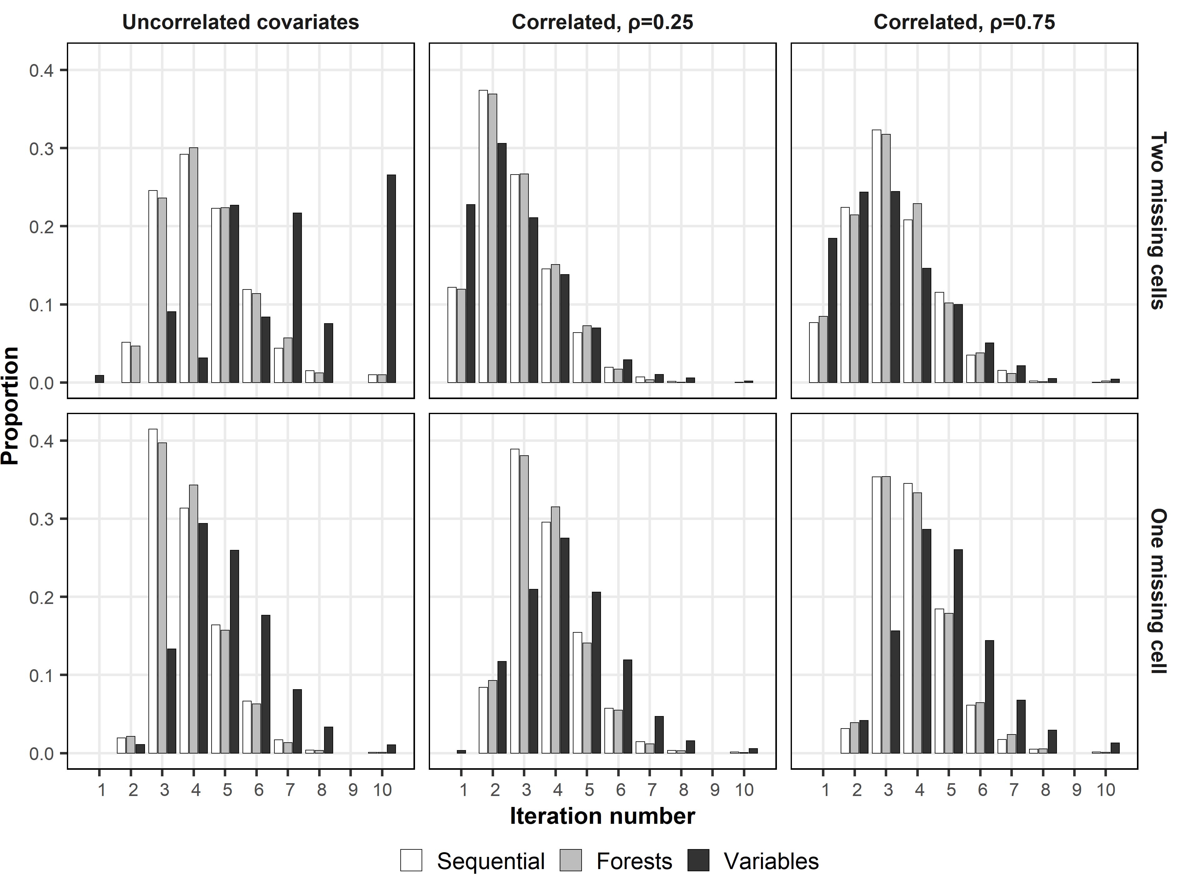
Figure 1: Number of iterations for different parallel modes in different data generation settings and missing patterns

The number of iterations of imputation with the “variables” parallel strategy was very different (p<0.001 across all scenarios, Fisher’s exact test) from the other two strategies for all eight data scenarios, while sequential imputation and parallel “forests” strategies were more similar. For the parallel “forests” and sequential strategies, most imputation runs stopped at two to four iterations with only a small number of runs (<0.25% overall) reaching the maximum number of ten loops. For the “variables” parallel imputation, however, imputation often require larger number of iterations even for data with one missing cell per observation (median no. of iterations = 3, 4 for two missing cells, one missing cell, respectively.) Note also that with two missing cells per observation, an exceedingly large proportion of runs (26.5%) stopped at the maximum iteration number for the “variables” strategy (Fig. 1).

3.2 Relative bias of sample mean

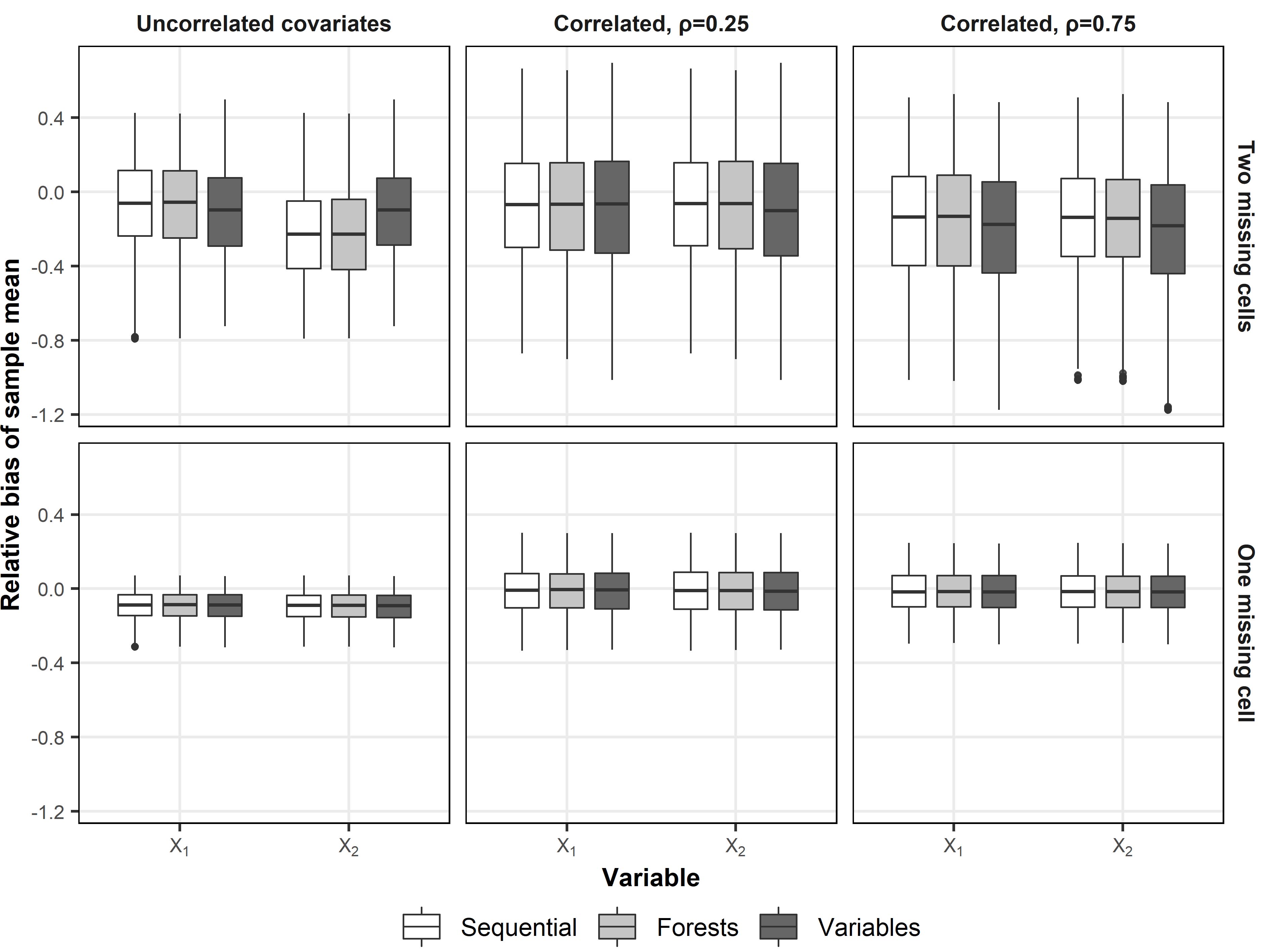
Figure 2: Relative bias of the estimated means of variables

The “variables” parallel imputation strategy resulted in more biased mean estimates in datasets with multiple missing cells per observation. With two missing cells per observation for the “uncorrelated covariates” scenario, the “variables” strategy had an additional downward relative bias when estimating the mean of $X_{1}$ (median = -9.8%) compared with the sequential (median = -6.1%, p<0.001) and “forests” (median = -5.5%, p<0.001) strategies, while for $X_{2}$ an additional upward relative bias was introduced (median = -22.8%, -22.8%, -9.7% for “sequential”, “forests”, “variables”, respectively). For weakly correlated data, the sample mean of $X_{1}$ was similar (median = -6.9%, -6.7%, -6.5%), but for $X_{2}$ a downward bias was introduced by “variables” (median = -6.3%, -6.3%, -10.0%). For strongly correlated data, the “variables” strategy produced biased downward sample means of $X_{1}$ (median = -13.5%, -13.2%, -17.5%), as well as $X_{2}$ (median = -13.7%, -14.2%, -18.2%). When there was only one missing cell per observation, the relative bias of the sample mean was similar across the three strategies (Fig. 2).

3.3 Relative bias of standard derivation

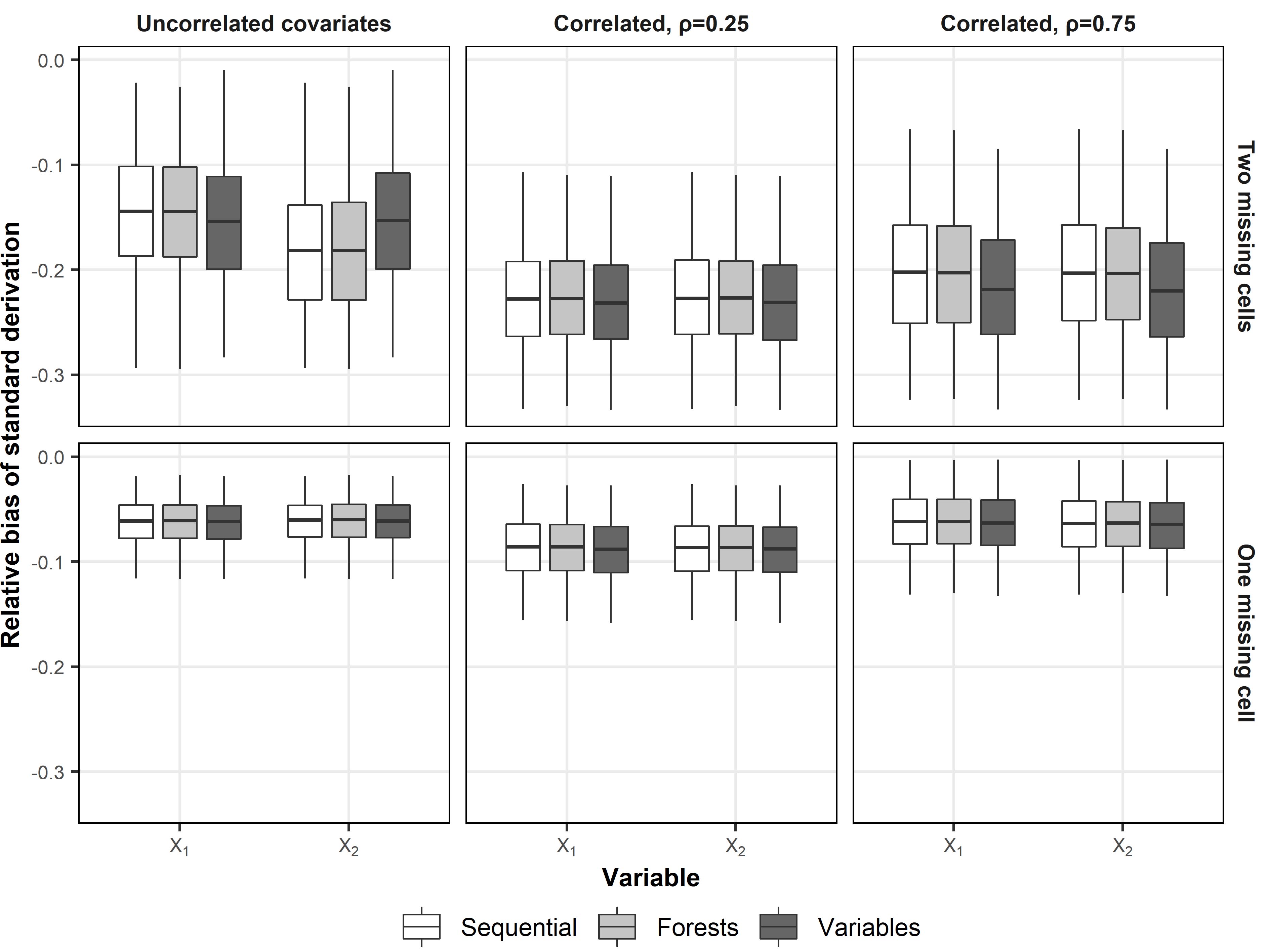
Figure 3: Relative bias of standard derivations of variables

For estimating the standard derivation, all three strategies were systematically biased downward. The results of the sequential and “forests” strategies were similar, with the “variables” strategy yielding slightly more biased estimates (Fig. 3). For example, with two missing cells per observation, the median relative biases for $X_{1}$ and $X_{2}$ were -14.4%, -14.4%, -15.4% and -18.2%, -18.1%, -15.3% for “sequential”, “forests”, “variables”, respectively, for the “uncorrelated covariates” scenario. While for strongly correlated data, the median relative biases for $X_{1}$ and $X_{2}$ were -20.2%, -20.3%, -21.9%, and -20.3%, -20.3%, -22.0%, respectively (Fig. 3).

3.4 Relative bias of regression coefficient estimates

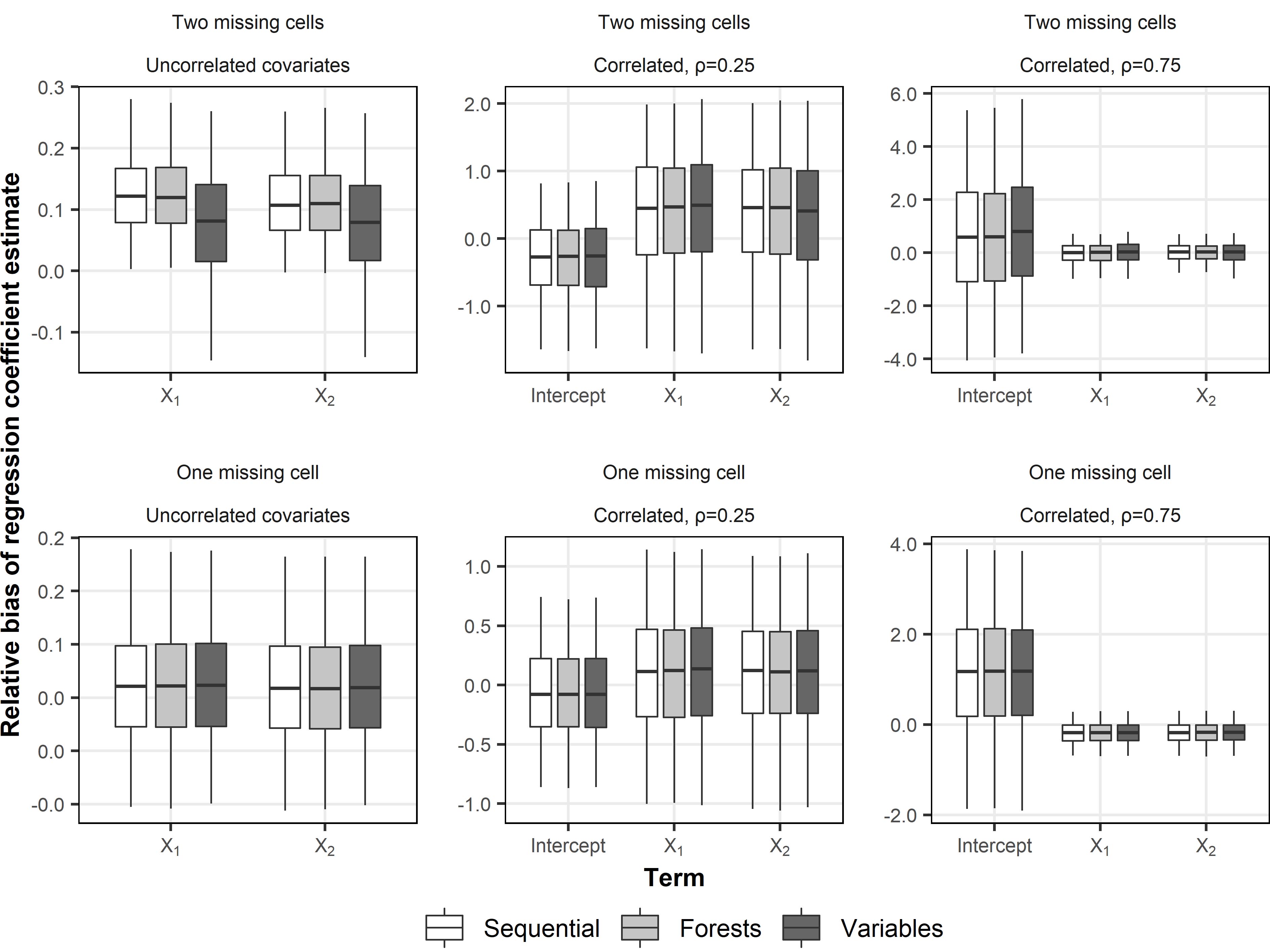
Figure 4: Relative bias of the estimated regression coefficients

MissForest led to biased regression coefficient estimates when covariates are outcome-dependent MAR, and the “variables” parallel strategy can cause additional bias. With two missing cells per observation, the “sequential” and “forests” strategies were similar for the “uncorrelated covariates” scenario, but the “variables” strategy produced additional downward relative bias ($X_{1}$: median = 12.1%, 12.0%, 8.1%, for “sequential”, “forests”, “variables”, respectively; $X_{2}$: median = 10.7%, 11.0%, 7.9%, respectively). For weakly correlated data, the median relative biases for coefficient estimates of (intercept, $X_{1}$, $X_{2}$) were (-16.4%, -15.8%, -15.5%), (9.0%, 9.4%, 9.9%), and (9.1%, 9.2%, 8.2%) for the “sequential”, “forests”, and “variables” strategies, respectively. While for strongly correlated data, the median relative biases for coefficient estimates of (intercept $X_{1}$, $X_{2}$) were (8.3%, 8.5%, 11.5%), (0.2%, 0.4%, 1.1%), and (1.3%, 1.2%, 0.9%), respectively. For datasets with only one missing cell per observation, imputation using different parallel strategies gave similar results (Fig. 4).

3.5 Bias of correlation between covariates

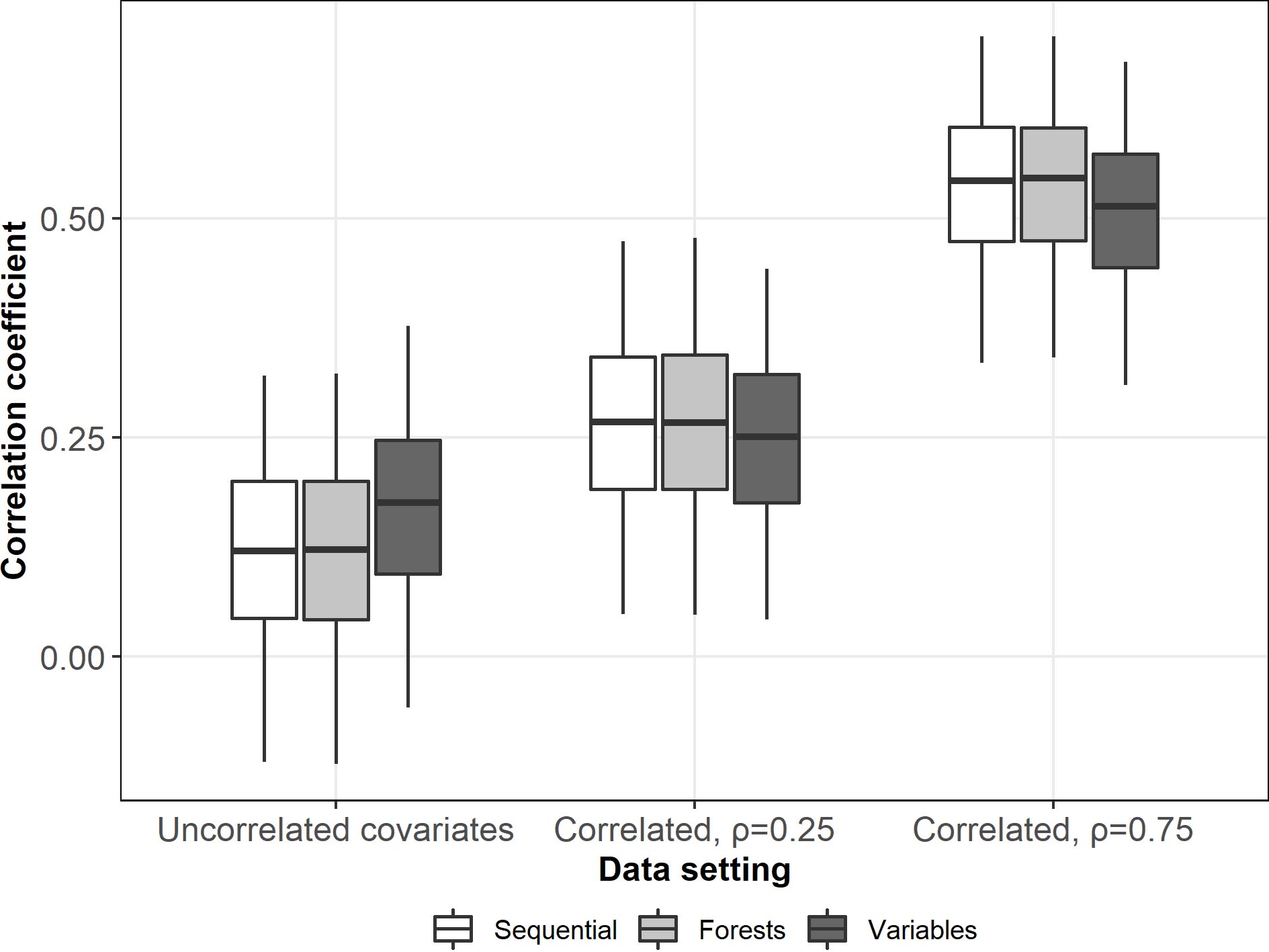
Figure 5: Bias of correlation between covariates

The choice of strategy influenced the correlation between the imputed covariates. With two missing cells per observation, all three strategies produced inflated correlations between $X_{1}$ and $X_{2}$ for the “uncorrelated covariates” scenario (Fig. 5) but the “variables” parallel strategy resulted in the most biased correlation estimates (median = 0.18 compared to 0.12, for both “sequential” and “forests” strategies). For weakly correlated data, the correlation coefficients were similar, but for highly correlated data the correlations were biased downward with the “variables” strategy yielding the lowest estimate (median = 0.51 compared to 0.55 and 0.54 for “sequential” and “forests”, respectively).

3.6 Normalized root mean squared error

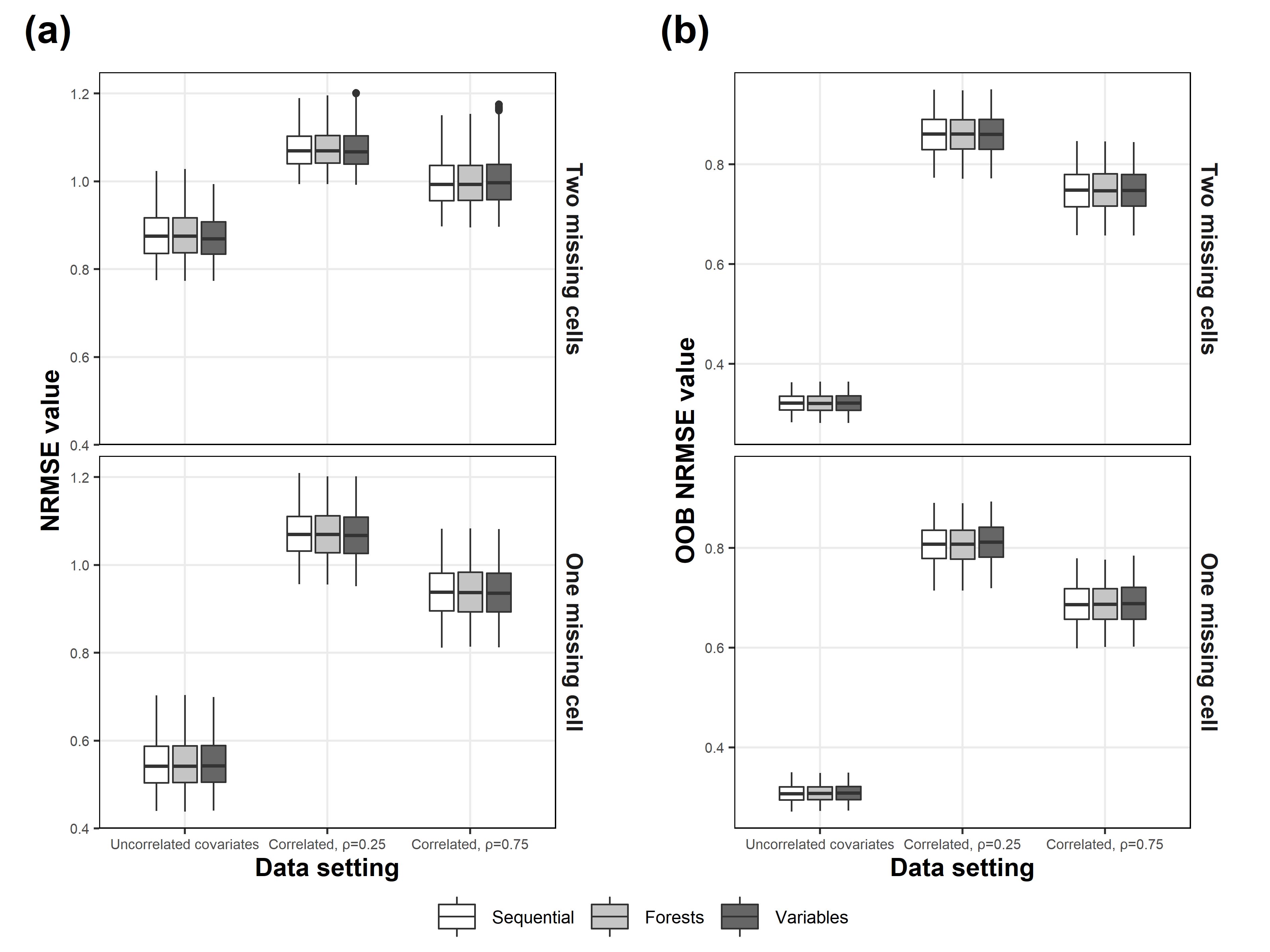
Figure 6: Normalized root mean squared errors (NRMSE) in final imputed data, (a) NRMSE calculated based on true data; (b) out-of-bag (OOB) errors calculated from OOB observations

The NRMSE values for all three strategies appeared similar, regardless of whether they were calculated based on the original data (Fig. 6a), or from the out-of-bag (OOB) values (Fig. 6b).

4 Discussion

This study examines the parallel algorithms of the RF-based imputation method missForest and documents for the first time their influence on imputation results. By distributing imputation computation to multiple computing processes, reduction in time consumption can be achieved with multi-core processors. In the “forests” parallel strategy, the imputation for a single variable was parallelized, and in the “variables” mode, the single iteration of imputation for different variables was parallelized. Depending on the data structures, our findings indicate that the “variables” strategy can lead to variations in the final imputation results compared with the original missForest “sequential” algorithm. The “variables” strategy yielded additional upward or downward biases when estimating covariate means, correlation between covariates, and regression coefficients. This can harm reproducibility and may even lead to false inference. Moreover, the little variation in NRMSE values between the different strategies may give a false sense of consistency between them. This also highlights the fact that evaluating imputation results based solely on NRMSE values can lead to unreliable conclusions.

The difference in results between the two parallel strategies is a consequence of their different computing processes. In the parallel “forests” strategy, the imputation of the current variable is based on the latest state of the imputation dataset, and the observations of the previously imputed variable are updated before the start of the imputation of the current variable. The computation of a single tree in an ensemble is also done independent of other trees, so this parallel strategy should be similar to the “sequential” strategy that computes all the trees in an ensemble using a single processor rather than multiple processors. On the other hand, in the parallel “variables” strategy the imputation of different variables is done in parallel such that their computation is based on the same previously updated imputed dataset rather than variable-wise sequentially updated imputed datasets. This implies that imputed results are not updated until one cycle of imputation is finished for all the variables imputed in parallel. Therefore, the imputation of the variables within a single iteration can no longer be considered sequential, resulting in different final imputed values from the “sequential” strategy.

The simulations in this study focused on “long” data where the number of observations is larger than the number of variables in the dataset. However, for “wide” data with large number of variables, the impact of the non-sequential updating of imputed values in the “variables” parallel strategy can be even larger, especially when missing values are scattered across multiple variables with low inter-correlations. It should be noted that the data settings in this study were designed to accentuate the differences and consequences of the two different parallel strategies. In practice, however, datasets like the simulated data in this study may not be suited for parallel computation as they are not large enough in terms of number of variables or observations. Also, the parallelization algorithm can lead to additional time cost, resulting in more computational time than expected.

This study highlights the importance of thorough testing of computational algorithms. In particular, it is the lack of technical details in the official missForest documentations that prompted this investigation. Machine learning methods like random forests are computationally intensive. Likewise, their application to big data problems will necessitate the use of parallel computation algorithms, but developers and users of such statistical software may be wise to devise simple simulation experiments to test and compare the algorithms before using them for data analyses. Finally, although we focused on the missForest method the lessons learned here is not peculiar to it, and other iterative imputation methods (e.g., MICE) may be faced with similar problems when adapted for parallel computation.

5 Conclusions

The problem of using parallel computation has been brought into the forefront with this study’s investigation of the two parallel strategies implemented in missForest. It is expected that the proliferation of large datasets and complex computational methods will continue to fuel the use of parallel algorithms. The careful analysis of these algorithms is therefore especially important, and the documentation of these algorithms should include sufficient technical details and test experiments to inform researchers of potential problems.

References

- [1] Liaw A, Wiener M (2002) Classification and regression by randomForest. R news 2:18-22
- [2] Mayer M (2019) missRanger: Fast Imputation of Missing Values. CRAN. https://CRAN.R-project.org/package=missRanger. Accessed 1 January 2020
- [3] R Core Team (2019) R: A language and environment for statistical computing.
- [4] Ramosaj B, Pauly M (2019) Predicting missing values: a comparative study on non-parametric approaches for imputation. Computational Statistics 34:1741-1764 https://doi.org/10.1007/s00180-019-00900-3
- [5] Schouten RM, Lugtig P, Vink G (2018) Generating missing values for simulation purposes: a multivariate amputation procedure. Journal of Statistical Computation and Simulation 88:2909-2930 https://doi.org/10.1080/00949655.2018.1491577
- [6] Searle SR, Gruber MHJ (2016) Linear Models. 2nd edn. John Wiley & Sons, Hoboken, New Jersey
- [7] Shah AD, Bartlett JW, Carpenter J, Nicholas O, Hemingway H (2014) Comparison of random forest and parametric imputation models for imputing missing data using MICE: a CALIBER study. American Journal of Epidemiology 179:764-774 https://doi.org/10.1093/aje/kwt312
- [8] Stekhoven DJ (2013) missForest: Nonparametric Missing Value Imputation using Random Forest, R package version 1.4. CRAN. https://CRAN.R-project.org/package=missForest. Accessed 1 January 2020
- [9] Stekhoven DJ, Buhlmann P (2012) MissForest–non-parametric missing value imputation for mixed-type data. Bioinformatics 28:112-118 https://doi.org/10.1093/bioinformatics/btr597
- [10] Tang F, Ishwaran H (2017) Random Forest Missing Data Algorithms. Statistical Analysis and Data Mining 10:363-377 https://doi.org/10.1002/sam.11348
- [11] van Buuren S, Groothuis-Oudshoorn K (2011) mice: Multivariate Imputation by Chained Equations in R. Journal of Statistical Software 45 https://doi.org/10.18637/jss.v045.i03
- [12] Waljee AK et al. (2013) Comparison of imputation methods for missing laboratory data in medicine. BMJ Open 3 https://doi.org/10.1136/bmjopen-2013-002847