A stabilizer free weak Galerkin element method with supercloseness of order two
Abstract
The weak Galerkin (WG) finite element method is an effective and flexible general numerical techniques for solving partial differential equations. A simple weak Galerkin finite element method is introduced for second order elliptic problems. First we have proved that stabilizers are no longer needed for this WG element. Then we have proved the supercloseness of order two for the WG finite element solution. The numerical results confirm the theory.
keywords:
weak Galerkin, finite element methods, weak gradient, second-order elliptic problems, stabilizer free, supercloseness.AMS:
Primary: 65N15, 65N30; Secondary: 35J501 Introduction
The weak Galerkin finite element method is an effective and flexible numerical techniques for solving partial differential equations. It is a natural extension of the standard Galerkin finite element method where classical derivatives were substituted by weakly defined derivatives on functions with discontinuity. The WG method was first introduced in [13, 14] and then has been applied to solve various partial differential equations [2, 4, 3, 5, 7, 8, 9, 10, 6, 11, 12, 15].
The main idea of weak Galerkin finite element methods is the use of weak functions and their corresponding weak derivatives in algorithm design. For the second order elliptic equation, weak functions have the form of with inside of each element and on the boundary of the element. Both and can be approximated by polynomials in and respectively, where stands for an element and the edge or face of , and are non-negative integers with possibly different values. Weak derivatives are defined for weak functions in the sense of distributions. For example, one may approximate a weak gradient in the polynomial space . Various combination of leads to different weak Galerkin methods tailored for specific partial differential equations.
A stabilizing/penalty term is often used in finite element methods with discontinuous approximations to enforce connection of discontinuous functions across element boundaries. Removing stabilizers from weak Galerkin finite element methods will simplify formulations and reduce programming complexity significantly. Stabilizer free WG finite element methods have been studied in [16, 1, 17]. The idea is to increase the connectivity of a weak function cross element boundary by raising the degree of polynomials for computing weak derivatives. In [16], it has been proved that for a WG element , the condition of guarantees a stabilizer free WG method, where is the number of edges/faces of an element.
In this paper, a WG finite element is investigated for second order elliptic problems. This new WG finite element leads to a stabilizer free weak Galerkin formulation. In addition, we have proved order two supercloseness for the WG finite element solution, i.e. the WG solution approaches to the projection of the true solution with the convergence rates two order higher than the optimal convergence rate in both an energy norm and the norm. The numerical results show high accuracy of the WG method and confirm our theory.
For simplicity, we demonstrate the idea by using the second order elliptic problem that seeks an unknown function satisfying
| (1.1) | |||||
| (1.2) |
where is a polytopal domain in , denotes the gradient of the function , and is a symmetric matrix-valued function in . We shall assume that there exist two positive numbers such that
| (1.3) |
Here is understood as a column vector and is the transpose of .
The paper is organized as follows. In Section 2, we shall describe a new WG scheme. Section 3 will discussion the well posedness of the WG scheme. The error analysis for the WG solutions in an energy norm and in the norms will be investigated in Section 4 and Section 5 respectively. In Section 7, we shall present some numerical results that confirm the theory developed in earlier sections. Finally, technical proof of Lemma 3.1 will be presented in Appendix.
2 Weak Galerkin Finite Element Schemes
Let be a shape regular partition of the domain consisting of triangles. Denote by the set of all edges in , and let be the set of all interior edges. For every element , we denote by its diameter and mesh size for .
First, we adopt the following notations,
For a given integer , define a weak Galerkin finite element space associated with as follows
| (2.1) |
and its subspace is defined as
| (2.2) |
We would like to emphasize that any function has a single value on each edge .
For , a weak gradient is a piecewise vector valued polynomial such that on each , satisfies
| (2.3) |
In the above equation, we let and if .
Let and be the two element-wise defined projections onto and with respectively for each . Define . Let be the element-wise defined projection onto on each element .
Weak Galerkin Algorithm 1.
We will need the following lemma in the error analysis.
Lemma 1.
Let , then on any ,
| (2.5) | |||||
| (2.6) |
Proof.
For any function , the following trace inequality holds true (see [14] for details):
| (2.7) |
3 Well Posedness
For any , define two semi-norms
| (3.1) | |||||
| (3.2) |
It follows from (1.3) that there exist two positive constants and such that
| (3.3) |
We introduce a discrete semi-norm as follows:
| (3.4) |
It is easy to show that defines a norm in .
Next we will show that also defines a norm in by proving the equivalence of and in . First we need the following lemma.
The proof of the following lemma is long and can be found in Appendix.
Lemma 2.
For any , we have
| (3.5) |
Lemma 3.
There exist two positive constants and such that for any , we have
| (3.6) |
Proof.
Lemma 4.
The weak Galerkin finite element scheme (2.4) has a unique solution.
4 Error Estimates in Energy Norm
The goal of this section is to establish some error estimates for the weak Galerkin finite element solution arising from (2.4). For simplicity of analysis, we assume that the coefficient tensor in (1.1) is a piecewise constant matrix with respect to the finite element partition . The result can be extended to variable tensors without any difficulty, provided that the tensor is piecewise sufficiently smooth.
Let . Next we derive an error equation that satisfies. Define a bilinear form by
Lemma 5.
For any , the error satisfies the following equation
| (4.1) |
Proof.
Theorem 6.
Let be the weak Galerkin finite element solution of (2.4). Assume the exact solution . Then, there exists a constant such that
| (4.5) |
5 Error Estimates in Norm
The standard duality argument is used to obtain error estimate. Recall . The considered dual problem seeks satisfying
| (5.1) |
Assume that the following -regularity holds
| (5.2) |
Theorem 7.
Proof.
By testing (5.1) with we obtain
| (5.4) | |||||
where we have used the fact that on . Setting and in (4.3) yields
| (5.5) |
Substituting (5.5) into (5.4) gives
| (5.6) | |||||
Using the Cauchy-Schwarz inequality and (2.7), we obtain
| (5.7) | |||||
From the trace inequality (2.7) and the definition of , we have
and
Combining the above two estimates with (5.7) gives
| (5.8) |
6 Numerical Experiments
6.1 Example 1
Consider problem (1.1) with and . The source term and the boundary value are chosen so that the exact solution is (non-symmetric, nonzero boundary value)
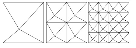
In this example, we use uniform grids shown in Figure 6.1. In Table 6.1, we list the errors and the orders of convergence. We can see that we do have two orders of superconvergence in both norms.
| level | rate | rate | ||
|---|---|---|---|---|
| by the - WG finite element | ||||
| 5 | 0.5867E-06 | 3.99 | 0.6420E-04 | 2.99 |
| 6 | 0.3677E-07 | 4.00 | 0.8043E-05 | 3.00 |
| 7 | 0.2310E-08 | 3.99 | 0.1021E-05 | 2.98 |
| by the - WG finite element | ||||
| 3 | 0.6072E-05 | 4.90 | 0.2699E-03 | 3.95 |
| 4 | 0.1938E-06 | 4.97 | 0.1704E-04 | 3.99 |
| 5 | 0.6113E-08 | 4.99 | 0.1071E-05 | 3.99 |
| by the - WG finite element | ||||
| 2 | 0.1513E-04 | 5.50 | 0.4704E-03 | 4.45 |
| 3 | 0.2397E-06 | 5.98 | 0.1519E-04 | 4.95 |
| 4 | 0.3750E-08 | 6.00 | 0.4819E-06 | 4.98 |
6.2 Example 2
We solve problem (1.1) where and
The source term and the boundary value are chosen so that the exact solution is
We use same meshes as Example 1. The result is listed in Table 6.2. The superconvergence phenomena are same as those in Example 1, i.e., 2 orders of superconvergence in both norm and three-bar norm.
| level | rate | rate | ||
|---|---|---|---|---|
| by the - WG finite element | ||||
| 5 | 0.5487E-06 | 3.95 | 0.1023E-03 | 2.97 |
| 6 | 0.3471E-07 | 3.98 | 0.1288E-04 | 2.99 |
| 7 | 0.2182E-08 | 3.99 | 0.1621E-05 | 2.99 |
| by the - WG finite element | ||||
| 3 | 0.4230E-05 | 4.69 | 0.3492E-03 | 3.84 |
| 4 | 0.1440E-06 | 4.88 | 0.2261E-04 | 3.95 |
| 5 | 0.4680E-08 | 4.94 | 0.1432E-05 | 3.98 |
| by the - WG finite element | ||||
| 2 | 0.8490E-05 | 5.34 | 0.5269E-03 | 4.62 |
| 3 | 0.1436E-06 | 5.89 | 0.1738E-04 | 4.92 |
| 4 | 0.2296E-08 | 5.97 | 0.5534E-06 | 4.97 |
6.3 Example 3
Consider problem (1.1) with and . The source term and the boundary value are chosen so that the exact solution is
In this example, we use nonuniform grids shown in Figure 6.2. In Table 6.3, we list the errors and the orders of convergence. We can see that we do have two orders of superconvergence in both norms.
| level | rate | rate | ||
|---|---|---|---|---|
| by the - WG finite element | ||||
| 5 | 0.4530E-05 | 4.00 | 0.1130E-02 | 3.00 |
| 6 | 0.2830E-06 | 4.00 | 0.1411E-03 | 3.00 |
| 7 | 0.1768E-07 | 4.00 | 0.1762E-04 | 3.00 |
| by the - WG finite element | ||||
| 5 | 0.4027E-07 | 5.00 | 0.1389E-04 | 4.00 |
| 6 | 0.1256E-08 | 5.00 | 0.8671E-06 | 4.00 |
| 7 | 0.3920E-10 | 5.00 | 0.5415E-07 | 4.00 |
| by the - WG finite element | ||||
| 4 | 0.2138E-07 | 6.01 | 0.4534E-05 | 5.01 |
| 5 | 0.3308E-09 | 6.01 | 0.1407E-06 | 5.01 |
| 6 | 0.4979E-11 | 6.05 | 0.4378E-08 | 5.01 |
6.4 Example 4
Consider problem (1.1) with and . The source term and the boundary value are chosen so that the exact solution is
We use tetrahedral meshes shown in Figure 6.3. The results of the - weak Galerkin finite element methods are listed in Table 6.4. The superconvergence phenomena are same as those in 2D, in first three examples, two orders of superconvergence.
| level | rate | rate | ||
|---|---|---|---|---|
| by the - WG finite element | ||||
| 1 | 0.0748126 | 0.0 | 0.9508644 | 0.0 |
| 2 | 0.0120779 | 2.6 | 0.1909763 | 2.3 |
| 3 | 0.0010535 | 3.5 | 0.0280478 | 2.8 |
| 4 | 0.0000726 | 3.9 | 0.0036750 | 2.9 |
| 5 | 0.0000047 | 4.0 | 0.0004657 | 3.0 |
| 6 | 0.0000003 | 4.0 | 0.0000584 | 3.0 |
| by the - WG finite element | ||||
| 1 | 0.0106321 | 0.0 | 0.4099718 | 0.0 |
| 2 | 0.0019247 | 2.5 | 0.0537392 | 2.9 |
| 3 | 0.0000721 | 4.7 | 0.0038352 | 3.8 |
| 4 | 0.0000024 | 4.9 | 0.0002476 | 4.0 |
| 5 | 0.0000001 | 5.0 | 0.0000156 | 4.0 |
| by the - WG finite element | ||||
| 1 | 0.0170645 | 0.0 | 0.3318098 | 0.0 |
| 2 | 0.0003554 | 5.6 | 0.0128696 | 4.7 |
| 3 | 0.0000062 | 5.8 | 0.0004504 | 4.8 |
| 4 | 0.0000001 | 6.0 | 0.0000145 | 5.0 |
Appendix
We prove Lemma 2 in the Appendix. First we need the following lemmas.
Lemma 8.
Let
and
be two positive definite quadratic forms, where , and . Then so that is a positive definite quadratic form for each .
Proof.
We need to show that there exists a such that is positive definite for . Since is positive definite, , where is also symmetric positive definite with symmetric positive definite inverse. Thus
Let . Then is positive definite and thus
| (.1) |
where and is an orthogonal matrix. Thus we can write
| (.2) |
Obviously, is positive definite when and so is . ∎
Lemma 9.
For any , then
| (.3) |
where .
Proof.
Without loss of generality, we may assume that the vertices of are ,
and the other edge of is , where . Denote .
Let be unit tangents to , respectively; be linear functions such that . Let
and
where are such that
| (.4) |
By setting in in (.4), we know such exist and are unique. Then
Scale if necessary so that
where is the unit outwards normal vector of .
Since ,
Similarly
It follows from the shape regularity assumptions that the slope of , satisfies for some . Since ,
Note that . Write
Let . Then
are positive definite quadratic forms in . Note that
is a positive definite quadratic form. Similarly,
is also a positive definite quadratic form. So by Lemma 8,
and
Thus
for some . It is worthwhile to note that this is independent of in some sense. If we want to change the scale from to , we only need to replace by . Because of the dimensional differences of the two sides, will be replace by . Thus after a scaling we have
∎
Lemma 10.
Let and be such as in Lemma 9, then
| (.5) |
Proof.
Without loss, we may assume that and are as shown in the Figure .5, where .
Let us assume that . If follows from Lemma 9 that
We want to show
| (.6) |
first. Let , then on . Denote by the unite outer ward normal vector to . Let and be unit tangent vectors to and respectively. Let
where . Write
where . We want to show that for each , we can find a unique so that
| (.7) |
To do that we set and . Then
which implies that
This implies the existence and the uniqueness of . Now let
where
Thus
since and . Without loss, we assume . Let be such that . Write
Write
and
such that
Then
and thus
| (.8) |
Further, let
Then
Thus, implies . Next we want to choose so that
| (.9) |
To see if (.9) has a unique solution, we set . Then . Thus (.9) becomes
It is easy to see that . Thus
Similarly, we can show that
Now let’s look at . Since
| (.10) |
Let
where is such that
and is extended to . Then
Similarly
By (.10)
Thus
implies
Let
where . Let , write , where is the coefficient vector of . Then
Thus is a positive definite quadratic form in . Similarly
are positive definite quadratic forms in , where are variables in the first quadratic forms and are variables in the second quadratic forms, respectively. Note that the leading coefficients of and are the same. To keep those variables independent, we remove that coefficient from and let . Write , then
where is positive definite. Since is uniquely determined by and by solving a linear system,
where is positive semi-definite. Since implies , is positive definite. By Lemma 8 and a scaling argument,
∎
References
- [1] A. Al-Taweel and X. Wang, A note on the optimal degree of the weak gradient of the stabilizer free weak Galerkin finite element method, Applied Numerical Mathematics, 150 (2020), 444-451.
- [2] X. Hu, L. Mu and X. Ye, A weak Galerkin finite element method for the Navier-Stokes equations on polytopal meshes, J. of Computational and Applied Mathematics, 362 (2019), 614-625.
- [3] R. Lin, X. Ye, S. Zhang and P. Zhu, A weak Galerkin finite element method for singularly perturbed convection-diffusion-reaction problems, SINUM, 56 (2018) 1482-1497.
- [4] G. Lin, J. Liu, L.Mu and X. Ye, weak Galerkin finite element methods for Darcy flow: Anisotropy and heterogeneity, J. Comput. Phy. 276 (2014), 422-437.
- [5] L. Mu, J. Wang and X. Ye, weak Galerkin finite element method for the Helmholtz equation with large wave number on polytopal meshes, IMA J. Numer. Anal. 35 (2015), 1228-1255.
- [6] L. Mu, J. Wang, and X. Ye, A stable numerical algorithm for the Brinkman equations by weak Galerkin finite element methods, J. of Computational Physics, 273 (2014), 327-342.
- [7] L. Mu, J. Wang and X. Ye, A weak Galerkin finite element method for biharmonic equations on polytopal meshes, Numer. Meth. Partial Diff. Eq. 30 (2014), 1003-1029.
- [8] L. Mu, J. Wang and X. Ye, Weak Galerkin finite element method for second-order elliptic problems on polytopal meshes, Int. J. Numer. Anal. Model. 12 (2015) 31-53.
- [9] L. Mu, J. Wang, X. Ye and S. Zhang, A weak Galerkin finite element method for the Maxwell equations, J. Sci. Comput. 65 (2015), 363-386.
- [10] L. Mu, J. Wang, X. Ye and S. Zhao, A new weak Galerkin finite element method for elliptic interface problems, J. Comput. Phy. 325 (2016), 157-173.
- [11] S. Shields, J. Li and E.A. Machorro, Weak Galerkin methods for time-dependent Maxwell’s equations, Comput. Math. Appl. 74 (2017) 2106-2124.
- [12] C. Wang and J. Wang, Discretization of div–curl systems by weak Galerkin finite element methods on polyhedral partitions, J. Sci. Comput. 68 (2016) 1144-1171.
- [13] J. Wang and X. Ye, A weak Galerkin finite element method for second-order elliptic problems. J. Comput. Appl. Math. 241 (2013), 103-115.
- [14] J. Wang and X. Ye, A Weak Galerkin mixed finite element method for second-order elliptic problems, Math. Comp., 83 (2014), 2101-2126.
- [15] J. Wang and X. Ye, A weak Galerkin finite element method for the Stokes equations, Adv. in Comput. Math. 42 (2016) 155-174.
- [16] X. Ye and S. Zhang, A stabilizer-free weak Galerkin finite element method on polytopal meshes, J. Comput. Appl. Math., 372 (2020), 112699, arXiv:1906.06634.
- [17] X. Ye, S. Zhang and Y. Zhu, Stabilizer-free weak Galerkin methods for monotone quasilinear elliptic PDEs, Results in Applied Mathematics, https://doi.org/10.1016/j.rinam.2020.100097