Unique continuation from the edge of a crack

Abstract.

In this work we develop an Almgren type monotonicity formula for a class of elliptic equations in a domain with a crack, in the presence of potentials satisfying either a negligibility condition with respect to the inverse-square weight or some suitable integrability properties. The study of the Almgren frequency function around a point on the edge of the crack, where the domain is highly non-smooth, requires the use of an approximation argument, based on the construction of a sequence of regular sets which approximate the cracked domain. Once a finite limit of the Almgren frequency is shown to exist, a blow-up analysis for scaled solutions allows us to prove asymptotic expansions and strong unique continuation from the edge of the crack.

Keywords. Crack singularities; monotonicity formula; unique continuation; blow-up analysis.

MSC2020 classification. 35J15, 35C20, 74A45.

1. Introduction and statement of the main results

This paper presents a monotonicity approach to the study of the asymptotic behavior and unique continuation from the edge of a crack for solutions to the following class of elliptic equations

$$\left\{\begin{aligned} -\Delta u(x)&=f(x)u(x)&&\text{in $\Omega\setminus\Gamma$},\\ u&=0&&\text{on}\ \Gamma,\end{aligned}\right.$$ (1.1)

where $\Omega\subset\mathbb{R}^{N+1}$ is a bounded open domain, $\Gamma\subset\mathbb{R}^{N}$ is a closed set, $N\geq 2$, and the potential $f$ satisfies either a negligibility condition with respect to the inverse-square weight, see assumptions (H1-1)-(H1-3), or some suitable integrability properties, see assumptions (H2-1)-(H2-5) below.

We recall that the strong unique continuation property is said to hold for a certain class of equations if no solution, besides possibly the zero function, has a zero of infinite order. Unique continuation principles for solutions to second order elliptic equations have been largely studied in the literature since the pioneering contribution by Carleman [6], who derived unique continuation from some weighted a priori inequalities. Garofalo and Lin in [20] studied unique continuation for elliptic equations with variable coefficients introducing an approach based on the validity of doubling conditions, which in turn depend on the monotonicity property of the Almgren type frequency function, defined as the ratio of scaled local energy over mass of the solution near a fixed point, see [4].

Once a strong unique continuation property is established and infinite vanishing order for non-trivial solutions is excluded, the problem of estimating and possibly classifying all admissible vanishing rates naturally arises. For quantitative uniqueness and bounds for the maximal order of vanishing obtained by monotonicity methods we cite e.g. [23]; furthermore, a precise description of the asymptotic behavior together with a classification of possible vanishing orders of solutions was obtained for several classes of problems in [15, 16, 17, 18, 19], by combining monotonicity methods with blow-up analysis for scaled solutions.

The problem of unique continuation from boundary points presents peculiar additional difficulties, as the derivation of monotonicity formulas is made more delicate by the interference with the geometry of the domain. Moreover the possible vanishing orders of solutions are affected by the regularity of the boundary; e.g. in [15] the asymptotic behavior at conical singularities of the boundary has been shown to depend of the opening of the vertex. We cite [2, 3, 15, 24, 29] for unique continuation from the boundary for elliptic equations under homogeneous Dirichlet conditions. We also refer to [28] for unique continuation and doubling properties at the boundary under zero Neumann conditions and to [11] for a strong unique continuation result from the vertex of a cone under non-homogeneous Neumann conditions.

The aforementioned papers concerning unique continuation from the boundary require the domain to be at least of Dini type. With the aim of relaxing this kind of regularity assumptions, the present paper investigates unique continuation and classification of the possible vanishing orders of solutions at edge points of cracks breaking the domain, which are then highly irregular points of the boundary.

Elliptic problems in domains with cracks arise in elasticity theory, see e.g. [9, 22, 25]. The high non-smoothness of domains with slits produces strong singularities of solutions to elliptic problems at edges of cracks; the structure of such singularities has been widely studied in the literature, see e.g. [7, 8, 12] and references therein. In particular, asymptotic expansions of solutions at edges play a crucial role in crack problems, since the coefficients of such expansions are related to the so called stress intensity factor, see e.g. [9].

A further reason of interest in the study of problem (1.1) can be found in its relation with mixed Dirichlet/Neumann boundary value problems. Indeed, if we consider an elliptic equation associated, on a flat portion of the boundary $\Lambda=\Lambda_{1}\cup\Lambda_{2}$, to a homogeneous Dirichlet boundary condition on $\Lambda_{1}$ and a homogeneous Neumann condition on $\Lambda_{2}$, an even reflection through the flat boundary $\Lambda$ leads to an elliptic equation satisfied in the complement of the Dirichlet region, which then plays the role of a crack, see Figure 1; the edge of the crack corresponds to the Dirichlet-Neumann junction of the original problem. In [14] unique continuation and asymptotic expansions of solutions for planar mixed boundary value problems at Dirichlet-Neumann junctions were obtained via monotonicity methods; the present paper is in part motivated by the aim of extending to higher dimensions the monotonicity formula obtained in [14] in the 2-dimensional case, together with its applications to unique continuation. For some regularity results for second-order elliptic problems with mixed Dirichlet-Neumann type boundary conditions we refer to [21, 27] and references therein.

(a) Mixed Dirichlet/Neumann boundary conditions on a flat portion of the boundary

(b) After an even reflection the Dirichlet region becomes a crack

Figure 1. A motivation from mixed Dirichlet/Neumann boundary value problems

In the generalization of the Almgren type monotonicity formula of [14] to dimensions greater than 2, some new additional difficulties arise, besides the highly non-smoothness of the domain: the positive dimension of the edge, a stronger interference with the geometry of the domain, and some further technical issues, related e.g. to the lack of conformal transformations straightening the edge. In particular, the proof of the monotonicity formula is based on the differentiation of the Almgren quotient defined in (4.9), which in turn requires a Pohozaev type identity formally obtained by testing the equation with the function $\nabla u\cdot x$; however our domain with crack doesn’t verify the exterior ball condition (which ensures $L^{2}$-integrability of second order derivatives, see [1]) and $\nabla u\cdot x$ could be not sufficiently regular to be an admissible test function.

In this article a new technique, based on an approximation argument, is developed to overcome the aforementioned difficulty: we construct first a sequence of domains which approximate $\Omega\setminus\Gamma$, satisfying the exterior ball condition and being star-shaped with respect to the origin, and then a sequence of solutions of an approximating problem on such domains, converging to the solution of the original problem with crack. For the approximating problems enough regularity is available to establish a Pohozaev type identity, with some remainder terms due to interference with the boundary, whose sign can nevertheless be recognized thanks to star-shapeness conditions. Then, passing to the limit in Pohozaev identities for the approximating problems, we obtain inequality (3.11), which is enough to estimate from below the derivative of the Almgren quotient and to prove that such quotient has a finite limit at $0$ (Lemma 4.7). Once a finite limit of the Almgren frequency is shown to exist, a blow-up analysis for scaled solutions allows us to prove strong unique continuation and asymptotics of solutions.

In order to state the main results of the present paper, we start by introducing our assumptions on the domain. For $N\geq 2$, we consider the set

$$\Gamma=\{(x^{\prime},x_{N})=(x_{1},\dots,x_{N-1},x_{N})\in\mathbb{R}^{N}:\,x_{N}\geq g(x^{\prime})\},$$

where $g\colon\mathbb{R}^{N-1}\to\mathbb{R}$ is a function such that

$$g(0)=0,\quad\nabla g(0)=0,$$ (1.2)

$$g\in C^{2}(\mathbb{R}^{N-1}).$$ (1.3)

Let us observe that assumption (1.2) is not a restriction but just a selection of our coordinate system and, from (1.2) and (1.3), it follows that

$$|g(x^{\prime})|=O(|x^{\prime}|^{2})\quad\text{as $|x^{\prime}|\rightarrow 0^{+}$}.$$ (1.4)

Moreover we assume that

$$g(x^{\prime})-x^{\prime}\cdot\nabla g(x^{\prime})\geq 0$$ (1.5)

for any $x^{\prime}\in B^{\prime}_{\hat{R}}:=\{x^{\prime}\in\mathbb{R}^{N-1}:|x^{\prime}|<\hat{R}\}$, for some $\hat{R}>0$. This condition says that $\overline{\mathbb{R}^{N}\setminus\Gamma}$ is star-shaped with respect to the origin in a neighbourood of 0. It is satisfied for instance if the function $g$ is concave in a neighborhood of the origin.

We are interested in studying the following boundary value problem

$$\left\{\begin{aligned} -\Delta u&=f\,u&&\text{in}\ B_{\hat{R}}\setminus\Gamma,\\ u&=0&&\text{on}\ \Gamma,\end{aligned}\right.$$ (1.6)

where $B_{\hat{R}}=\{x\in\mathbb{R}^{N+1}:|x|<\hat{R}\}$, for some function $f\colon B_{\hat{R}}\to\mathbb{R}$ such that $f$ is measurable and bounded in $B_{\hat{R}}\setminus B_{\delta}$ for every $\delta\in(0,\hat{R})$. We consider two alternative sets of assumptions: we assume either that

$$\lim_{r\rightarrow 0^{+}}\xi_{f}(r)=0,$$ (H1-1)

$$\frac{\xi_{f}(r)}{r}\in L^{1}(0,\hat{R}),\quad\frac{1}{r}\int_{0}^{r}\frac{\xi_{f}(s)}{s}\,ds\in L^{1}(0,\hat{R}),$$ (H1-2)

where the function $\xi_{f}$ is defined as

$$\xi_{f}(r):=\sup_{x\in\overline{B_{r}}}|x|^{2}|f(x)|\quad\text{for any $r\in(0,\hat{R})$},$$ (H1-3)

or that

$$\lim_{r\rightarrow 0^{+}}\eta(r,f)=0,$$ (H2-1)

$$\frac{\eta(r,f)}{r}\in L^{1}(0,\hat{R}),\quad\frac{1}{r}\int_{0}^{r}\frac{\eta(s,f)}{s}\,ds\in L^{1}(0,\hat{R}),$$ (H2-2)

and

$$\nabla f\in L^{\infty}_{\mathrm{loc}}(B_{\hat{R}}\setminus\{0\}),$$ (H2-3)

$$\frac{\eta(r,\nabla f\cdot x)}{r}\in L^{1}(0,\hat{R}),\quad\frac{1}{r}\int_{0}^{r}\frac{\eta(s,\nabla f\cdot x)}{s}\,ds\in L^{1}(0,\hat{R}),$$ (H2-4)

where

$$\eta(r,h)=\sup_{u\in H^{1}(B_{r})\setminus\{0\}}\frac{\int_{B_{r}}|h|u^{2}\,dx}{\int_{B_{r}}|\nabla u|^{2}\,dx+\frac{N-1}{2r}\int_{\partial B_{r}}|u|^{2}\,dS},$$ (H2-5)

for every $r\in(0,\hat{R}),\,h\in L^{\infty}_{\mathrm{loc}}(B_{\hat{R}}\setminus\{0\})$.

Conditions (H1-1)-(H1-3) are satisfied e.g. if $|f(x)|=O(|x|^{-2+\delta})$ as $|x|\rightarrow 0$ for some $\delta>0$, whereas assumptions (H2-1)-(H2-5) hold e.g. if $f\in W^{1,\infty}_{\mathrm{loc}}(B_{\hat{R}}\setminus\{0\})$ and $f,\nabla f\in L^{p}(B_{\hat{R}})$ for some $p>\frac{N+1}{2}$. We also observe that condition (H2-1) is satisfied if $f$ belongs to the Kato class $K_{n+1}$, see [13].

In order to give a weak formulation of problem (1.6), we introduce the space $H^{1}_{\Gamma}(B_{R})$ for every $R>0$, defined as the closure in $H^{1}(B_{R})$ of the subspace

$$C^{\infty}_{0,\Gamma}(\overline{B_{R}}):=\{u\in C^{\infty}(\overline{B_{R}}):u=0\ \text{in a neighborhood of}\ \Gamma\}.$$

We observe that actually

$$H^{1}_{\Gamma}(B_{R})=\{u\in H^{1}(B_{R}):\,\tau_{\Gamma}(u)=0\},$$

where $\tau_{\Gamma}$ denotes the trace operator on $\Gamma$, as one can easily deduce from [5], taking into account that the capacity of $\partial\Gamma$ in $\mathbb{R}^{N+1}$ is zero, since $\partial\Gamma$ is contained in a 2-codimensional manifold.

Hence we say that $u\in H^{1}(B_{\hat{R}})$ is a weak solution to (1.6) if

$$\left\{\begin{aligned} &u\in H^{1}_{\Gamma}(B_{\hat{R}}),\\ &\int_{B_{\hat{R}}}\nabla u(x)\cdot\nabla v(x)\,dx-\int_{B_{\hat{R}}}f(x)u(x)v(x)\,dx=0\quad\text{for any}\ v\in C_{c}^{\infty}(B_{\hat{R}}\setminus\Gamma).\end{aligned}\right.$$

In the classification of the possible vanishing orders and blow-up profiles of solutions, the following eigenvalue problem on the unit $N$-dimensional sphere with a half-equator cut plays a crucial role. Letting $\mathbb{S}^{N}=\{(x^{\prime},x_{N},x_{N+1}):|x^{\prime}|^{2}+x_{N}^{2}+x_{N+1}^{2}=1\}$ be the unit $N$-dimensional sphere and $\Sigma=\{(x^{\prime},x_{N},x_{N+1})\in\mathbb{S}^{N}:x_{N+1}=0\text{ and }x_{N}\geq 0\}$, we consider the eigenvalue problem

$$\left\{\begin{aligned} -\Delta_{\mathbb{S}^{N}}\psi&=\mu\,\psi&&\text{on }\mathbb{S}^{N}\setminus\Sigma,\\ \psi&=0&&\text{on }\Sigma.\end{aligned}\right.$$ (1.7)

We say that $\mu\in\mathbb{R}$ is an eigenvalue of (1.7) if there exists an eigenfunction $\psi\in H^{1}_{0}(\mathbb{S}^{N}\setminus\Sigma)$, $\psi\not\equiv 0$, such that

$$\int_{\mathbb{S}^{N}}\nabla_{\mathbb{S}^{N}}\psi\cdot\nabla_{\mathbb{S}^{N}}\phi\,dS=\mu\int_{\mathbb{S}^{N}}\psi\phi\,dS$$

for all $\phi\in H^{1}_{0}(\mathbb{S}^{N}\setminus\Sigma)$. By classical spectral theory, (1.7) admits a diverging sequence of real eigenvalues with finite multiplicity $\{\mu_{k}\}_{k\geq 1}$; moreover these eigenvalues are explicitly given by the formula

$$\mu_{k}=\frac{k(k+2N-2)}{4},\quad k\in\mathbb{N}\setminus\{0\},$$ (1.8)

see Appendix A. For all $k\in\mathbb{N}\setminus\{0\}$, let $M_{k}\in\mathbb{N}\setminus\{0\}$ be the multiplicity of the eigenvalue $\mu_{k}$ and

$$\begin{split}\{Y_{k,m}\}_{m=1,2,\dots,M_{k}}\text{ be a $L^{2}(\mathbb{S}^{N})$-orthonormal basis}\\ \text{ of the eigenspace of \eqref{eq:1} associated to $\mu_{k}$}.\end{split}$$ (1.9)

In particular $\{Y_{k,m}:k\in\mathbb{N}\setminus\{0\},m=1,2,\dots,M_{k}\}$ is an orthonormal basis of $L^{2}(\mathbb{S}^{N})$.

The main result of this paper provides an evaluation of the behavior at 0 of weak solutions $u\in H^{1}(B_{\hat{R}})$ to the boundary value problem (1.6).

Theorem 1.1.

Let $N\geq 2$ and $u\in H^{1}(B_{\hat{R}})\setminus\{0\}$ be a non-trivial weak solution to (1.6), with $f$ satisfying either assumptions (H1-1)-(H1-3) or (H2-1)-(H2-5). Then, there exist $k_{0}\in\mathbb{N}$, $k_{0}\geq 1$, and an eigenfunction of problem (1.7) associated with the eigenvalue $\mu_{k_{0}}$ such that

$$\lambda^{-k_{0}/2}u(\lambda x)\rightarrow|x|^{k_{0}/2}\psi(x/|x|)\quad\text{as $\lambda\rightarrow 0^{+}$}$$ (1.10)

in $H^{1}(B_{1})$.

We mention that a strongest version of Theorem 1.1 will be given in Theorem 6.7.

As a direct consequence of Theorem 1.1 and the boundedness of eigenfunctions of (1.7) (see Appendix A), the following point-wise upper bound holds.

Corollary 1.2.

Under the same assumptions as in Theorem 1.1, let $u\in H^{1}(B_{\hat{R}})$ be a non-trivial weak solution to (1.6). Then, there exists $k_{0}\in\mathbb{N}$, $k_{0}\geq 1$, such that

$$u(x)=O(|x|^{k_{0}/2})\quad\text{as $|x|\rightarrow 0^{+}$}.$$

We observe that, due to the vanishing on the half-equator $\Sigma$ of the angular profile $\psi$ appearing in (1.10), we cannot expect the reverse estimate $|u(x)|\geq c|x|^{k_{0}/2}$ to hold for $x$ close to the origin.

A further relevant consequence of our asymptotic analysis is the following unique continuation principle, whose proof follows straightforwardly from Theorem 1.1.

Corollary 1.3.

Under the same assumptions as in Theorem 1.1, let $u\in H^{1}(B_{\hat{R}})$ be a weak solution to (1.6) such that $u(x)=O(|x|^{k})$ as $|x|\rightarrow 0$, for any $k\in\mathbb{N}$. Then $u\equiv 0$ in $B_{\hat{R}}$.

Theorem 6.7 will actually give a more precise description on the limit angular profile $\psi$: if $M_{k_{0}}\geq 1$ is the multiplicity of the eigenvalue $\mu_{k_{0}}$ and $\{Y_{k_{0},i}:1\leq i\leq M_{k_{0}}\}$ is as in (1.9), then the eigenfunction $\psi$ in (1.10) can be written as

$$\psi(\theta)=\sum_{i=1}^{m_{k_{0}}}\beta_{i}Y_{k_{0},i},$$ (1.11)

where the coefficients $\beta_{i}$ are given by the integral Cauchy-type formula (6.40).

The paper is organized as follows. In Section 2 we construct a sequence of problems on smooth sets approximating the cracked domain, with corresponding solutions converging to the solution of problem (1.6). In Section 3 we derive a Pohozaev type identity for the approximating problems and consequently inequality (3.11), which is then used in Section 4 to prove the existence of the limit for the Almgren type quotient associated to problem (1.6). In Section 5 we perform a blow-up analysis and prove that scaled solutions converge in some suitable sense to a homogeneous limit profile, whose homogeneity order is related to the eigenvalues of problem (1.7) and whose angular component is shown to be as in (1.11) in Section 6, where an auxiliary equivalent problem with a straightened crack is constructed. Finally, in the appendix we derive the explicit formula (1.8) for the eigenvalues of problem (1.7).

Notation. We list below some notation used throughout the paper.

• For all $r>0$, $B_{r}$ denotes the open ball $\{x=(x^{\prime},x_{N},x_{N+1})\in\mathbb{R}^{N+1}:|x|<r\}$ in $\mathbb{R}^{N+1}$ with radius $r$ and center at 0.

• For all $r>0$, $\overline{B_{r}}=\{x=(x^{\prime},x_{N},x_{N+1})\in\mathbb{R}^{N+1}:|x|\leq r\}$ denotes the closure of $B_{r}$.

• For all $r>0$, $B^{\prime}_{r}$ denotes the open ball $\{x=(x^{\prime},x_{N})\in\mathbb{R}^{N}:|x|<r\}$ in $\mathbb{R}^{N}$ with radius $r$ and center at 0.

• $dS$ denotes the volume element on the spheres $\partial B_{r}$, $r>0$.
  

2. Approximation problem

We first prove a coercivity type result for the quadratic form associated to problem (1.6) in small neighbourhoods of $0$.

Lemma 2.1.

Let $f$ satisfy either (H1-1) or (H2-1). Then there exists $r_{0}\in(0,\hat{R})$ such that, for any $r\in(0,r_{0}]$ and $u\in H^{1}(B_{r})$,

$$\int_{B_{r}}(|\nabla u|^{2}-|f|u^{2})\,dx\geq\frac{1}{2}\int_{B_{r}}|\nabla u|^{2}\,dx-\omega(r)\int_{\partial B_{r}}u^{2}\,dS$$ (2.1)

and

$$r\omega(r)<\frac{N-1}{4},$$ (2.2)

where

$$\omega(r)=\begin{cases}\dfrac{2}{N-1}\dfrac{\xi_{f}(r)}{r},&\text{under assumption \eqref{xi0}},\\[10.0pt] \dfrac{N-1}{2}\dfrac{\eta(r,f)}{r},&\text{under assumption \eqref{eta0}}.\end{cases}$$ (2.3)

Remark 2.2.

For future reference, it is useful to rewrite (2.1) as

$$\int_{B_{r}}|f|u^{2}\,dx\leq\frac{1}{2}\int_{B_{r}}|\nabla u|^{2}\,dx+\omega(r)\int_{\partial B_{r}}u^{2}\,ds$$ (2.4)

for all $u\in H^{1}(B_{r})$ and $r\in(0,r_{0}]$.

The proof of Lemma 2.1 under assumption (H1-1) is based on the following Hardy type inequality with boundary terms, due to Wang and Zhu [30].

Lemma 2.3 ([30], Theorem 1.1).

For every $r>0$ and $u\in H^{1}(B_{r})$,

$$\int_{B_{r}}|\nabla u(x)|^{2}\,dx+\frac{N-1}{2r}\int_{\partial B_{r}}|u(x)|^{2}\,dS\geq\biggl{(}\frac{N-1}{2}\biggr{)}^{2}\int_{B_{r}}\frac{|u(x)|^{2}}{|x|^{2}}\,dx.$$ (2.5)

Proof of Lemma 2.1.

Let us first prove the lemma under assumption (H1-1). To this purpose, let $r_{0}\in(0,\hat{R})$ be such that

$$\frac{4\xi_{f}({r})}{(N-1)^{2}}<\frac{1}{2}\quad\text{for all }r\in(0,r_{0}].$$ (2.6)

Using the definition of $\xi_{f}(r)$ (H1-3) and (2.5), we have that for any $r\in(0,\hat{R})$ and $u\in H^{1}(B_{r})$

$$\int_{B_{r}}|f|u^{2}\,dx\leq\xi_{f}(r)\int_{B_{r}}\frac{|u(x)|^{2}}{|x|^{2}}\,dx\leq\frac{4\xi_{f}(r)}{(N-1)^{2}}\biggl{[}\int_{B_{r}}|\nabla u|^{2}\,dx+\frac{N-1}{2r}\int_{\partial B_{r}}u^{2}\,dS\biggr{]}.$$ (2.7)

Thus, for every $0<r\leq r_{0}$, from (2.6) and (2.7), we obtain that

$$\begin{split}\int_{B_{r}}\big{(}|\nabla u|^{2}-|f|u^{2}\big{)}\,dx&\geq\biggl{(}1-\frac{4\xi_{f}(r)}{(N-1)^{2}}\biggr{)}\int_{B_{r}}|\nabla u|^{2}\,dx-\frac{2}{N-1}\frac{\xi_{f}(r)}{r}\int_{\partial B_{r}}u^{2}\,ds\\ &\geq\frac{1}{2}\int_{B_{r}}|\nabla u|^{2}\,dx-\frac{2}{N-1}\frac{\xi_{f}(r)}{r}\int_{\partial B_{r}}u^{2}\,ds\end{split}$$

and this completes the proof of (2.1) under assumption (H1-1).

Now let us prove the lemma under assumption (H2-1). Let $r_{0}\in(0,\hat{R})$ be such that

$$\eta(r,f)<\frac{1}{2}\quad\text{for all $r\in(0,r_{0}]$}.$$ (2.8)

From the definition of $\eta(r,f)$ (H2-5) it follows that for any $r\in(0,\hat{R})$ and $u\in H^{1}(B_{r})$

$$\int_{B_{r}}|f|u^{2}\,dx\leq\eta(r,f)\biggl{[}\int_{B_{r}}|\nabla u|^{2}\,dx+\frac{N-1}{2r}\int_{\partial B_{r}}u^{2}\,dS\biggr{]}.$$ (2.9)

Thus, for every $0<r\leq r_{0}$, from (2.8) and (2.9) we deduce that

$$\begin{split}\int_{B_{r}}\big{(}|\nabla u|^{2}-|f|u^{2}\big{)}\,dx&\geq(1-\eta(r,f))\int_{B_{r}}|\nabla u|^{2}\,dx-\frac{N-1}{2}\frac{\eta(r,f)}{r}\int_{\partial B_{r}}u^{2}\,dS\\ &\geq\frac{1}{2}\int_{B_{r}}|\nabla u|^{2}\,dx-\frac{N-1}{2}\frac{\eta(r,f)}{r}\int_{\partial B_{r}}u^{2}\,ds,\end{split}$$

hence concluding the proof of (2.1) under assumption (H2-1).

We observe that estimate (2.2) follows from the definition of $\omega$ in (2.3), (2.6), and (2.8). ∎

Now we are going to construct suitable regular sets which are star-shaped with respect to the origin and which approximate our cracked domain. In order to do this, for any $n\in\mathbb{N}\setminus\{0\}$ let $f_{n}\colon\mathbb{R}\to\mathbb{R}$ be defined as

$$f_{n}(t)=\begin{cases}n|t|+\frac{1}{n}e^{\frac{2n^{2}|t|}{n^{2}|t|-2}},&\text{if }|t|<2/n^{2},\\ n|t|,&\text{if }|t|\geq 2/n^{2},\end{cases}$$

so that $f_{n}\in C^{2}(\mathbb{R})$, $f_{n}(t)\geq n|t|$ and $f_{n}$ increases for all $t>0$ and decreases for all $t<0$; furthermore

$$f_{n}(t)-t\,f^{\prime}_{n}(t)\geq 0\quad\text{for every }t\in\mathbb{R}.$$ (2.10)

For all $r>0$ we define

$$\tilde{B}_{{r},n}=\{(x^{\prime},x_{N},x_{N+1})\in B_{r}:\,x_{N}<g(x^{\prime})+f_{n}(x_{N+1})\},$$ (2.11)

see Figure 2.

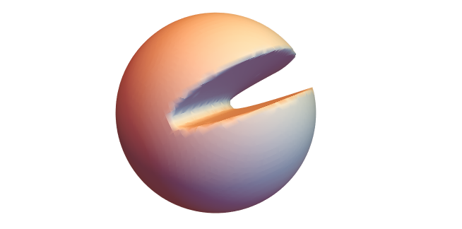
(a) The set $\tilde{B}_{r,n}$

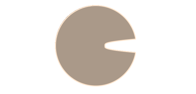
(b) Section of $\tilde{B}_{r,n}$

Figure 2. Approximating domains

Let $\tilde{\gamma}_{r,n}\subset\partial\tilde{B}_{r,n}$ be the subset of $B_{r}$ defined as

$$\tilde{\gamma}_{r,n}=\{(x^{\prime},x_{N},x_{N+1})\in B_{r}:\,x_{N}=g(x^{\prime})+f_{n}(x_{N+1})\}$$

and $\tilde{S}_{r,n}$ denote the set given by $\partial\tilde{B}_{r,n}\setminus\tilde{\gamma}_{r,n}$. We note that, for any fixed $r>0$, the set $\tilde{\gamma}_{r,n}$ is not empty and $\tilde{B}_{r,n}\neq B_{r}$ provided $n$ is sufficiently large.

Lemma 2.4.

Let $0<r\leq\hat{R}$. Then, for all $n\in{\mathbb{N}}\setminus\{0\}$, the set $\tilde{B}_{r,n}$ is star-shaped with respect to the origin, i.e. $x\cdot\nu\geq 0$ for a.e. $x\in\partial\tilde{B}_{r,n}$, where $\nu$ is the outward unit normal vector.

Proof.

If $\tilde{\gamma}_{r,n}$ is empty, then $\tilde{B}_{r,n}=B_{r}$ and the conclusion is obvious. Let $\tilde{\gamma}_{r,n}$ be not empty.

The thesis is trivial if one considers a point $x\in\tilde{S}_{r,n}$.

If $x\in\tilde{\gamma}_{r,n}$, then $x=(x^{\prime},g(x^{\prime})+f_{n}(x_{N+1}),x_{N+1})$ and the outward unit normal vector at this point is given by

$$\nu(x)=\frac{(-\nabla g(x^{\prime}),1,-f^{\prime}_{n}(x_{N+1}))}{\sqrt{1+|f^{\prime}_{n}(x_{N+1})|^{2}+|\nabla g(x^{\prime})|^{2}}},$$

hence we have that

$$x\cdot\nu(x)=\frac{g(x^{\prime})-\nabla g(x^{\prime})\cdot x^{\prime}+f_{n}(x_{N+1})-x_{N+1}\ f^{\prime}_{n}(x_{N+1})}{\sqrt{1+|f^{\prime}_{n}(x_{N+1}|^{2}+|\nabla g(x^{\prime})|^{2}}}\geq 0$$

since $g(x^{\prime})-\nabla g(x^{\prime})\cdot x^{\prime}\geq 0$ by assumption (1.5) and $f_{n}(x_{N+1})-x_{N+1}\,f^{\prime}_{n}(x_{N+1})\geq 0$ by (2.10). ∎

From now on, we fix $u\in H^{1}(B_{\hat{R}})\setminus\{0\}$, a non-trivial weak solution to problem (1.6), with $f$ satisfying either (H1-1)-(H1-3) or (H2-1)-(H2-5). Since $u\in H^{1}_{\Gamma}(B_{\hat{R}})$, there exists a sequence of functions $g_{n}\in C^{\infty}_{0,\Gamma}(\overline{B_{\hat{R}}})$ such that $g_{n}\rightarrow u$ in $H^{1}(B_{\hat{R}})$. We can choose the functions $g_{n}$ in such a way that

$$g_{n}(x_{1},\dots,x_{N},x_{N+1})=0\quad\text{if $(x_{1},\cdots,x_{N})\in\Gamma$ and $|x_{N+1}|\leq\frac{\tilde{C}}{n}$},$$ (2.12)

with

$$\tilde{C}>\sqrt{2(r_{0}^{2}+M^{2})},\quad\text{where }M=\mathrm{max}\{|g(x^{\prime})|:|x^{\prime}|\leq r_{0}\}.$$ (2.13)

Remark 2.5.

We observe that $g_{n}\equiv 0$ in $B_{r_{0}}\setminus\tilde{B}_{r_{0},n}$. Indeed, if $x=(x^{\prime},x_{N},x_{N+1})\in B_{r_{0}}\setminus\tilde{B}_{r_{0},n}$, then

$$x_{N}\geq g(x^{\prime})+f_{n}(x_{N+1})>g(x^{\prime}),$$

so that $(x^{\prime},x_{N})\in\Gamma$. Moreover

$$x_{N}\geq f_{n}(x_{N+1})+g(x^{\prime})\geq n|x_{N+1}|-M,$$

with $M$ as in (2.13). Hence either $|x_{N+1}|\leq\frac{M}{n}$ or $r_{0}^{2}\geq x_{N}^{2}\geq(n|x_{N+1}|-M)^{2}\geq\frac{n^{2}}{2}|x_{N+1}|^{2}-M^{2}$. Thus $|x_{N+1}|\leq\frac{\sqrt{2(r_{0}^{2}+M^{2})}}{n}<\frac{\tilde{C}}{n}$, if we choose $\tilde{C}$ as in (2.13). Then $g_{n}(x)=0$ in view of (2.12).

Now we construct a sequence of approximated solutions $\{u_{n}\}_{n\in\mathbb{N}}$ on the sets $\tilde{B}_{r_{0},n}$. For each fixed $n\in\mathbb{N}$, we claim that there exists a unique weak solution $u_{n}$ to the boundary value problem

$$\left\{\begin{aligned} -\Delta u_{n}&=fu_{n}&&\text{in}\ \tilde{B}_{{r_{0}},n},\\ u_{n}&=g_{n}&&\text{on}\ \partial\tilde{B}_{{r_{0}},n}.\end{aligned}\right.$$ (2.14)

Letting

$$v_{n}:=u_{n}-g_{n},$$

we have that $u_{n}$ weakly solves (2.14) if and only if $v_{n}\in H^{1}(\tilde{B}_{{r_{0}},n})$ is a weak solution to the homogeneous boundary value problem

$$\left\{\begin{aligned} -\Delta v_{n}-fv_{n}&=fg_{n}+\Delta g_{n}&&\text{in}\ \tilde{B}_{{r_{0}},n},\\ v_{n}&=0&&\text{on}\ \partial\tilde{B}_{{r_{0}},n},\end{aligned}\right.$$ (2.15)

i.e.

$$\left\{\begin{aligned} &v_{n}\in H^{1}_{0}(\tilde{B}_{{r_{0}},n}),\\ &\int_{\tilde{B}_{{r_{0}},n}}(\nabla v_{n}\cdot\nabla\phi-fv_{n}\phi)\,dx=\int_{\tilde{B}_{{r_{0}},n}}(fg_{n}+\Delta g_{n})\phi\,dx\quad\text{for any}\ \phi\in H^{1}_{0}(\tilde{B}_{{r_{0}},n}).\end{aligned}\right.$$

Lemma 2.6.

Let $r_{0}$ be as in Lemma 2.1. Then, for all $n\in\mathbb{N}$, problem (2.15) has one and only one weak solution $v_{n}\in H^{1}_{0}(\tilde{B}_{{r_{0}},n})$, where $\tilde{B}_{{r_{0}},n}$ is defined in (2.11).

Proof.

Let us consider the bilinear form

$$a(v,w)=\int_{\tilde{B}_{{r_{0}},n}}(\nabla v\cdot\nabla w-fvw)\,dx,$$

for every $v,w\in H^{1}_{0}(\tilde{B}_{{r_{0}},n})$. Lemma 2.1 implies that $a$ is coercive on $H^{1}_{0}(\tilde{B}_{{r_{0}},n})$. Furthermore, from estimate (2.4) we easily deduce that $a$ is continuous. The thesis then follows from the Lax-Milgram Theorem. ∎

Proposition 2.7.

Under the same assumptions of Lemma 2.6, there exists a positive constant $C>0$ such that $\|v_{n}\|_{H^{1}_{0}(B_{r_{0}})}\leq C$ for every $n\in\mathbb{N}$, where $v_{n}$ is extended trivially to zero in $B_{r_{0}}\setminus\tilde{B}_{{r_{0}},n}$.

Proof.

Let us observe that $fg_{n}$ and $-\Delta g_{n}$ are bounded in $H^{-1}(B_{r_{0}})$ as a consequence of the boundedness of $g_{n}$ in $H^{1}(B_{r_{0}})$: indeed, using (2.4), one has that, for any $\phi\in H^{1}_{0}(B_{r_{0}})$,

$$\begin{split}\biggl{|}\int_{B_{r_{0}}}fg_{n}\phi\,dx\biggr{|}&\leq\biggl{(}\int_{B_{r_{0}}}|f|g_{n}^{2}\,dx\biggr{)}^{\frac{1}{2}}\biggl{(}\int_{B_{r_{0}}}|f|\phi^{2}\,dx\biggr{)}^{\frac{1}{2}}\\ &\leq\frac{1}{2}\biggl{(}\frac{1}{2}\int_{B_{r_{0}}}|\nabla g_{n}|^{2}\,dx+\omega(r_{0})\int_{\partial B_{r_{0}}}g_{n}^{2}\,ds\biggr{)}^{\frac{1}{2}}\biggl{(}\int_{B_{r_{0}}}|\nabla\phi|^{2}\,dx\biggr{)}^{\frac{1}{2}}\\ &\leq c_{1}\|g_{n}\|_{H^{1}(B_{r_{0}})}\|\phi\|_{H^{1}_{0}(B_{r_{0}})},\end{split}$$ (2.16)

for some $c_{1}>0$ independent on $n$ and $\phi$, and

$$\biggl{|}-\int_{B_{r_{0}}}\Delta g_{n}\phi\,dx\biggr{|}=\biggl{|}\int_{B_{r_{0}}}\nabla g_{n}\cdot\nabla\phi\,dx\biggr{|}\leq c_{2}\|g_{n}\|_{H^{1}(B_{r_{0}})}\|\phi\|_{H^{1}_{0}(B_{r_{0}})},$$ (2.17)

for some $c_{2}>0$ independent on $n$ and $\phi$. Thus from (2.15), (2.16), (2.17) and Lemma 2.1, it follows that

$$\begin{split}\|v_{n}\|^{2}_{H^{1}_{0}(B_{r_{0}})}&=\int_{B_{r_{0}}}|\nabla v_{n}|^{2}\,dx\leq 2\int_{B_{r_{0}}}(|\nabla v_{n}|^{2}-fv_{n}^{2})\,dx=2\int_{B_{r_{0}}}(fg_{n}+\Delta g_{n})v_{n}\,dx\\ &\leq 2(c_{1}+c_{2})\|g_{n}\|_{H^{1}(B_{r_{0}})}\|v_{n}\|_{H^{1}_{0}(B_{r_{0}})}\leq c_{3}\|v_{n}\|_{H^{1}_{0}(B_{r_{0}})},\end{split}$$

for some $c_{3}>0$ independent on $n$. This completes the proof. ∎

Proposition 2.8.

Under the same assumptions of Lemma 2.6, we have that $u_{n}\rightharpoonup u$ weakly in $H^{1}(B_{r_{0}})$, where $u_{n}$ is extended trivially to zero in $B_{r_{0}}\setminus\tilde{B}_{r_{0},n}$.

Proof.

We observe that the trivial extension to zero of $u_{n}$ in $B_{r_{0}}\setminus\tilde{B}_{r_{0},n}$ belongs to $H^{1}(B_{r_{0}})$ since the trace of $u_{n}$ on $\tilde{\gamma}_{r_{0},n}$ is null in view of Remark 2.5.

From Proposition 2.7 it follows that there exist $\tilde{v}\in H^{1}_{0}(B_{r_{0}})$ and a subsequence $\{v_{n_{k}}\}$ of $\{v_{n}\}$ such that $v_{n_{k}}\rightharpoonup\tilde{v}$ weakly in $H^{1}_{0}(B_{r_{0}})$. Then $u_{n_{k}}=v_{n_{k}}+g_{n_{k}}\rightharpoonup\tilde{u}$ weakly in $H^{1}(B_{r_{0}})$, where $\tilde{u}:=\tilde{v}+u$. Let $\phi\in C^{\infty}_{c}(B_{r_{0}}\setminus\Gamma)$. Arguing as in Remark 2.5, we can prove that $\phi\in H^{1}_{0}(\tilde{B}_{r_{0},n_{k}})$ for all sufficiently large $k$. Hence, from (2.14) it follows that, for all sufficiently large $k$,

$$\int_{B_{r_{0}}}\nabla u_{n_{k}}\cdot\nabla\phi\,dx=\int_{B_{r_{0}}}fu_{n_{k}}\phi\,dx,$$ (2.18)

where $u_{n_{k}}$ is extended trivially to zero in $B_{r_{0}}\setminus\tilde{B}_{r_{0},n_{k}}$. Passing to the limit in (2.18), we obtain that

$$\int_{B_{r_{0}}}\nabla\tilde{u}\cdot\nabla\phi\,dx=\int_{B_{r_{0}}}f\tilde{u}\phi\,dx$$

for every $\phi\in C^{\infty}_{c}(B_{r_{0}}\setminus\Gamma)$. Furthermore $\tilde{u}=u$ on $\partial B_{r_{0}}$ in the trace sense: indeed, due to compactness of the trace map $\gamma:H^{1}(B_{r_{0}})\to L^{2}(\partial B_{r_{0}})$, we have that $\gamma(u_{n_{k}})\rightarrow\gamma(\tilde{u})$ in $L^{2}(\partial B_{r_{0}})$ and $\gamma(u_{n_{k}})=\gamma(g_{n_{k}})\rightarrow\gamma(u)$ in $L^{2}(\partial B_{r_{0}})$, since $g_{n}\rightarrow u\ \text{in}\ H^{1}(B_{r_{0}})$.

Finally, we prove that $\tilde{u}\in H^{1}_{\Gamma}(B_{r_{0}})$. To this aim, let $\Gamma_{\delta}=\{(x^{\prime},x_{N})\in\mathbb{R}^{N}:\,x_{N}\geq g(x^{\prime})+\delta\}$ for every $\delta>0$. For every $\delta>0$ we have that $\Gamma_{\delta}\cap B_{r_{0}}\subset B_{r_{0}}\setminus\tilde{B}_{r_{0},n}$ provided $n$ is sufficiently large. Hence, since $u_{n}$ is extended trivially to zero in $B_{r_{0}}\setminus\tilde{B}_{r_{0},n}$, we have that, for every $\delta>0$, $u_{n}\in H^{1}_{\Gamma_{\delta}}(B_{r_{0}})$ provided $n$ is sufficiently large. Since $H^{1}_{\Gamma_{\delta}}(B_{r_{0}})$ is weakly closed in $H^{1}(B_{r_{0}})$, it follows that $\tilde{u}\in H^{1}_{\Gamma_{\delta}}(B_{r_{0}})$ for every $\delta>0$, and hence $\tilde{u}\in H^{1}_{\Gamma}(B_{r_{0}})$.

Thus $\tilde{u}$ weakly solves

$$\left\{\begin{aligned} -\Delta\tilde{u}&=f\tilde{u}&&\text{in}\ B_{r_{0}}\setminus\Gamma,\\ \tilde{u}&=u&&\text{on}\ \partial B_{r_{0}},\\ \tilde{u}&=0&&\text{on}\ \Gamma.\end{aligned}\right.$$

Now we consider the function $U:=\tilde{u}-u$: it weakly solves the following problem

$$\left\{\begin{aligned} -\Delta U&=fU&&\text{in}\ B_{r_{0}}\setminus\Gamma,\\ U&=0&&\text{on}\ \partial B_{r_{0}},\\ U&=0&&\text{on}\ \Gamma.\end{aligned}\right.$$ (2.19)

Testing equation (2.19) with $U$ itself and using Lemma 2.1, we obtain that

$$\frac{1}{2}\int_{B_{r_{0}}}|\nabla U|^{2}\,dx\leq\int_{B_{r_{0}}}(|\nabla U|^{2}-fU^{2})\,dx=0,$$

so that $U=0$, hence $u=\tilde{u}$. By Urysohn’s subsequence principle, we can conclude that $u_{n}\rightharpoonup u$ weakly in $H^{1}(B_{r_{0}})$. ∎

Our next aim is to prove strong convergence of the sequence $\{u_{n}\}_{n\in\mathbb{N}}$ to $u$ in $H^{1}(B_{r_{0}})$.

Proposition 2.9.

Under the same assumptions of Lemma 2.6, we have that $u_{n}\rightarrow u$ in $H^{1}(B_{r_{0}})$.

Proof.

From Proposition 2.8 we deduce that $v_{n}\rightharpoonup 0$ in $H^{1}(B_{r_{0}})$, hence testing (2.15) with $v_{n}$ itself, we have that

$$\begin{split}\int_{B_{r_{0}}}(|\nabla v_{n}|^{2}-fv_{n}^{2})\,dx&=\int_{\tilde{B}_{r_{0},n}}(|\nabla v_{n}|^{2}-fv_{n}^{2})\,dx\\ &=\int_{\tilde{B}_{r_{0},n}}(fg_{n}v_{n}-\nabla g_{n}\nabla v_{n})\,dx=\int_{B_{r_{0}}}(fg_{n}v_{n}-\nabla g_{n}\nabla v_{n})\,dx\rightarrow 0\end{split}$$

as $n\rightarrow\infty$. Thus, from Lemma 2.1, we deduce that $\|v_{n}\|_{H^{1}_{0}(B_{r_{0}})}\rightarrow 0$ as $n\rightarrow\infty$, hence $v_{n}\rightarrow 0$ in $H^{1}(B_{r_{0}})$. This yields that $u_{n}=g_{n}+v_{n}\rightarrow u$ in $H^{1}(B_{r_{0}})$. ∎

3. Pohozaev Identity

In this section we derive a Pohozaev type identity for $u_{n}$ in which we will pass to the limit using Proposition 2.9. For every $r\in(0,r_{0})$ and $v\in H^{1}(B_{r})$, we define

$$\mathcal{R}(r,v)=\begin{cases}{\displaystyle\int_{B_{r}}}fv(x\cdot\nabla v)\,dx,&\text{if $f$ satisfies \eqref{xi0}-\eqref{xi}},\\[10.0pt] \dfrac{r}{2}{\displaystyle\int_{\partial B_{r}}}f\,v^{2}\,dS-\dfrac{1}{2}{\displaystyle\int_{B_{r}}}\big{(}\nabla f\cdot x+(N+1)f\big{)}v^{2}\,dx,&\text{if $f$ satisfies \eqref{eta0}-\eqref{eta}}.\end{cases}$$

Lemma 3.1.

Let $0<r<r_{0}$. There exists $n_{0}=n_{0}(r)\in\mathbb{N}\setminus\{0\}$ such that, for all $n\geq n_{0}$,

$$-\frac{N-1}{2}\int_{\tilde{B}_{r,n}}|\nabla u_{n}|^{2}\,dx+\frac{r}{2}\int_{\tilde{S}_{r,n}}|\nabla u_{n}|^{2}\,dS\\ -\frac{1}{2}\int_{\tilde{\gamma}_{r,n}}\biggl{|}\frac{\partial u_{n}}{\partial\nu}\biggr{|}^{2}x\cdot\nu\,dS-r\int_{\tilde{S}_{r,n}}\biggl{|}\frac{\partial u_{n}}{\partial\nu}\biggr{|}^{2}\,dS-\mathcal{R}(r,u_{n})=0.$$ (3.1)

Proof.

Since $u_{n}$ solves (2.14) in the domain $\tilde{B}_{r_{0},n}$, which satisfies the exterior ball condition, and $fu_{n}\in L^{2}_{\text{loc}}(\tilde{B}_{r_{0},n}\setminus\{0\})$, by elliptic regularity theory (see [1]) we have that $u_{n}\in H^{2}(\tilde{B}_{r,n}\setminus B_{\delta})$ for all $r\in(0,r_{0})$, $n$ sufficiently large and all $\delta<r_{n}$, where $r_{n}$ is such that $B_{r_{n}}\subset\tilde{B}_{r,n}$. Since

$$\int_{0}^{r_{n}}\biggl{[}\int_{\partial B_{r}}\big{(}|\nabla u_{n}|^{2}+|f|u_{n}^{2}\big{)}\,dS\biggr{]}\,dr=\int_{B_{r_{n}}}\big{(}|\nabla u_{n}|^{2}+|f|u_{n}^{2}\big{)}\,dx<+\infty,$$

there exists a sequence $\{\delta_{k}\}_{k\in\mathbb{N}}\subset(0,r_{n})$ such that $\lim_{k\rightarrow\infty}\delta_{k}=0$ and

$$\delta_{k}\int_{\partial B_{\delta_{k}}}|\nabla u_{n}|^{2}\,dS\rightarrow 0,\quad\delta_{k}\int_{\partial B_{\delta_{k}}}|f|u_{n}^{2}\,dS\rightarrow 0\quad\text{as $k\rightarrow\infty$}.$$ (3.2)

Testing (2.14) with $x\cdot\nabla u_{n}$ and integrating over $\tilde{B}_{r,n}\setminus B_{\delta_{k}}$, we obtain that

$$-\int_{\tilde{B}_{r,n}\setminus B_{\delta_{k}}}\Delta u_{n}(x\cdot\nabla u_{n})\,dx=\int_{\tilde{B}_{r,n}\setminus B_{\delta_{k}}}fu_{n}(x\cdot\nabla u_{n})\,dx.$$ (3.3)

Integration by parts allows us to rewrite the first term in (3.3) as

$$\begin{split}-\int_{\tilde{B}_{r,n}\setminus B_{\delta_{k}}}\Delta u_{n}(x\cdot\nabla u_{n})\,dx=&\int_{\tilde{B}_{r,n}\setminus B_{\delta}}\nabla u_{n}\cdot\nabla(x\cdot\nabla u_{n})\,dx-r\int_{\tilde{S}_{r,n}}\biggl{|}\frac{\partial u_{n}}{\partial\nu}\biggr{|}^{2}\,dS\\ &-\int_{\tilde{\gamma}_{r,n}}\biggl{|}\frac{\partial u_{n}}{\partial\nu}\biggr{|}^{2}x\cdot\nu\,dS+\delta_{k}\int_{\partial B_{\delta_{k}}}\biggl{|}\frac{\partial u_{n}}{\partial\nu}\biggr{|}^{2}\,dS,\end{split}$$ (3.4)

where we used that $x=r\nu$ on $\tilde{S}_{r,n}$ and that the tangential component of $\nabla u_{n}$ on $\tilde{\gamma}_{r,n}$ equals zero, thus $\nabla u_{n}=\frac{\partial u_{n}}{\partial\nu}\nu$ on $\tilde{\gamma}_{r,n}$. Furthermore, by direct calculations, the first term in (3.4) can be rewritten as

$$\begin{split}\int_{\tilde{B}_{r,n}\setminus B_{\delta_{k}}}\nabla u_{n}\cdot\nabla(x\cdot\nabla u_{n})\,dx=&-\frac{N-1}{2}\int_{\tilde{B}_{r,n}\setminus B_{\delta_{k}}}|\nabla u_{n}|^{2}\,dx+\frac{r}{2}\int_{\tilde{S}_{r,n}}|\nabla u_{n}|^{2}\,dS\\ &+\frac{1}{2}\int_{\tilde{\gamma}_{r,n}}\biggl{|}\frac{\partial u_{n}}{\partial\nu}\biggr{|}^{2}x\cdot\nu\,dS-\frac{\delta_{k}}{2}\int_{\partial B_{\delta_{k}}}|\nabla u_{n}|^{2}\,dS.\end{split}$$ (3.5)

Taking into account (3.3), (3.4) and (3.5), we obtain that

$$-\frac{N-1}{2}\int_{\tilde{B}_{r,n}\setminus B_{\delta_{k}}}|\nabla u_{n}|^{2}\,dx+\frac{r}{2}\int_{\tilde{S}_{r,n}}|\nabla u_{n}|^{2}\,dS-\frac{1}{2}\int_{\tilde{\gamma}_{r,n}}\biggl{|}\frac{\partial u_{n}}{\partial\nu}\biggr{|}^{2}x\cdot\nu\,dS-r\int_{\tilde{S}_{r,n}}\biggl{|}\frac{\partial u_{n}}{\partial\nu}\biggr{|}^{2}\,dS\\ -\frac{\delta_{k}}{2}\int_{\partial B_{\delta_{k}}}|\nabla u_{n}|^{2}\,dS+\delta_{k}\int_{\partial B_{\delta_{k}}}\biggl{|}\frac{\partial u_{n}}{\partial\nu}\biggr{|}^{2}\,dS-\int_{\tilde{B}_{r,n}\setminus B_{\delta_{k}}}fu_{n}(x\cdot\nabla u_{n})\,dx=0.$$ (3.6)

Under assumptions (H1-1)-(H1-3), the Hardy inequality (2.5) implies that $f\,u_{n}(x\cdot\nabla u_{n})\in L^{1}(B_{r})$ and hence

$$\lim_{k\to\infty}\int_{\tilde{B}_{r,n}\setminus B_{\delta_{k}}}fu_{n}(x\cdot\nabla u_{n})\,dx=\lim_{k\to\infty}\int_{B_{r}\setminus B_{\delta_{k}}}fu_{n}(x\cdot\nabla u_{n})\,dx=\int_{B_{r}}fu_{n}(x\cdot\nabla u_{n})\,dx.$$ (3.7)

On the other hand, if (H2-1)-(H2-5) hold, we can use the Divergence Theorem to obtain that

$$\int_{\tilde{B}_{r,n}\setminus B_{\delta_{k}}}fu_{n}(x\cdot\nabla u_{n})\,dx\\ =\frac{r}{2}\int_{\tilde{S}_{r,n}}fu_{n}^{2}\,dS-\frac{1}{2}\int_{\tilde{B}_{r,n}\setminus B_{\delta_{k}}}\big{(}\nabla f\cdot x+(N+1)f\big{)}u_{n}^{2}\,dx-\frac{\delta_{k}}{2}\int_{\partial B_{\delta_{k}}}fu_{n}^{2}\,dS\\ =\frac{r}{2}\int_{\partial B_{r}}fu_{n}^{2}\,dS-\frac{1}{2}\int_{B_{r}\setminus B_{\delta_{k}}}\big{(}\nabla f\cdot x+(N+1)f\big{)}u_{n}^{2}\,dx-\frac{\delta_{k}}{2}\int_{\partial B_{\delta_{k}}}fu_{n}^{2}\,dS.$$ (3.8)

Since, under assumptions (H2-1)-(H2-5), $\big{(}\nabla f\cdot x+(N+1)f\big{)}u_{n}^{2}\in L^{1}(B_{r})$, we can pass to the limit as $k\to\infty$ in (3.8) taking into account also (3.2), thus obtaining that

$$\lim_{k\to\infty}\int_{\tilde{B}_{r,n}\setminus B_{\delta_{k}}}fu_{n}(x\cdot\nabla u_{n})\,dx=\frac{r}{2}\int_{\partial B_{r}}fu_{n}^{2}\,dS-\frac{1}{2}\int_{B_{r}}\big{(}\nabla f\cdot x+(N+1)f\big{)}u_{n}^{2}\,dx.$$ (3.9)

Letting $k\rightarrow+\infty$ in (3.6), by (3.2), (3.7), and (3.9), we obtain (3.1). ∎

Combining Lemma 3.1 with the fact that the domains $\tilde{B}_{r,n}$ (defined as in (2.11)) are star-shaped with respect to the origin, we deduce the following inequality.

Corollary 3.2.

Let $0<r<r_{0}$. There exists $n_{0}=n_{0}(r)\in\mathbb{N}\setminus\{0\}$ such that, for all $n\geq n_{0}$,

$$-\frac{N-1}{2}\int_{\tilde{B}_{r,n}}|\nabla u_{n}|^{2}\,dx+\frac{r}{2}\int_{\tilde{S}_{r,n}}|\nabla u_{n}|^{2}\,dS-r\int_{\tilde{S}_{r,n}}\biggl{|}\frac{\partial u_{n}}{\partial\nu}\biggr{|}^{2}\,dS-\mathcal{R}(r,u_{n})\geq 0.$$ (3.10)

Proof.

In view of (3.1), the left-hand side of (3.10) is equal to $\frac{1}{2}\int_{\tilde{\gamma}_{r,n}}\big{|}\frac{\partial u_{n}}{\partial\nu}\big{|}^{2}x\cdot\nu\,dS$, which is in fact non-negative, since $x\cdot\nu\geq 0$ on $\tilde{\gamma}_{r,n}$ by Lemma 2.4. ∎

Passing to the limit in (3.10) as $n\to\infty$, a similar inequality can be derived for $u$.

Proposition 3.3.

Let $u$ solve (1.6), with $f$ satisfying either (H1-1)-(H1-3) or (H2-1)-(H2-5). Then, for a.e. $r\in(0,r_{0})$, we have that

$$-\frac{N-1}{2}\int_{B_{r}}|\nabla u|^{2}\,dx+\frac{r}{2}\int_{\partial B_{r}}|\nabla u|^{2}\,dS-r\int_{\partial B_{r}}\biggl{|}\frac{\partial u}{\partial\nu}\biggr{|}^{2}\,dS-\mathcal{R}(r,u)\geq 0$$ (3.11)

and

$$\int_{B_{r}}|\nabla u|^{2}\,dx=\int_{B_{r}}fu^{2}\,dx+\int_{\partial B_{r}}u\frac{\partial u}{\partial\nu}\,dS.$$ (3.12)

Proof.

In order to prove (3.11), we pass to the limit inside inequality (3.10). As regards the first term, it is sufficient to observe that

$$\int_{\tilde{B}_{r,n}}|\nabla u_{n}|^{2}dx=\int_{B_{r}}|\nabla u_{n}|^{2}dx\rightarrow\int_{B_{r}}|\nabla u|^{2}dx\quad\text{as $n\rightarrow\infty$},$$

for each fixed $r\in(0,r_{0})$, as a consequence of Proposition 2.9. In order to deal with the second term, we observe that, by strong $H^{1}$-convergence of $u_{n}$ to $u$,

$$\lim_{n\rightarrow+\infty}\int_{0}^{r_{0}}\biggl{(}\int_{\partial B_{r}}|\nabla(u_{n}-u)|^{2}\,dS\biggr{)}\,dr=0.$$ (3.13)

Letting

$$F_{n}(r)=\int_{\partial B_{r}}|\nabla(u_{n}-u)|^{2}\,dS,$$

(3.13) implies that $F_{n}\rightarrow 0$ in $L^{1}(0,r_{0})$. Then there exists a subsequence $F_{n_{k}}$ such that $F_{n_{k}}(r)\rightarrow 0$ for a.e. $r\in(0,r_{0})$, hence

$$\int_{\tilde{S}_{r,n_{k}}}|\nabla u_{n_{k}}|^{2}\,dS=\int_{\partial B_{r}}|\nabla u_{n_{k}}|^{2}\,dS\rightarrow\int_{\partial B_{r}}|\nabla u|^{2}\,dS\quad\text{as $k\rightarrow\infty$}$$

for a.e. $r\in(0,r_{0})$. In a similar way, we obtain that

$$\int_{\tilde{S}_{r,n_{k}}}\biggl{|}\frac{\partial u_{n_{k}}}{\partial\nu}\biggr{|}^{2}dS\rightarrow\int_{\partial B_{r}}\biggl{|}\frac{\partial u}{\partial\nu}\biggr{|}^{2}dS\quad\text{as $k\rightarrow\infty$}.$$

It remains to prove the convergence of $\mathcal{R}(r,u_{n})$. Under the set of assumptions (H1-1)-(H1-3), we first write

$$\begin{split}\int_{B_{r}}|fu_{n}(x\cdot\nabla u_{n})&-fu(x\cdot\nabla u)|dx=\int_{B_{r}}|f(u_{n}-u)(x\cdot\nabla u_{n})-fux\cdot\nabla(u-u_{n})|dx\\ &\leq\int_{B_{r}}|f(u_{n}-u)(x\cdot\nabla u_{n})|dx+\int_{B_{r}}|fux\cdot\nabla(u-u_{n})|dx.\end{split}$$ (3.14)

The Hölder inequality, (2.5), and Proposition 2.9 imply that

$$\int_{B_{r}}|f(u_{n}-u)(x\cdot\nabla u_{n})|dx\leq\xi_{f}(r)\biggl{(}\int_{B_{r}}\frac{|u_{n}-u|^{2}}{|x|^{2}}dx\biggr{)}^{1/2}\biggl{(}\int_{B_{r}}|\nabla u_{n}|^{2}dx\biggr{)}^{1/2}\\ \leq\frac{2}{N-1}\xi_{f}(r)\biggl{(}\int_{B_{r}}|\nabla(u_{n}-u)|^{2}dx+\frac{N-1}{2r}\int_{\partial B_{r}}|u_{n}-u|^{2}dS\biggr{)}^{1/2}\biggl{(}\int_{B_{r}}|\nabla u_{n}|^{2}dx\biggr{)}^{1/2}\rightarrow 0$$

and

$$\int_{B_{r}}|fux\cdot\nabla(u_{n}-u)|dx\leq\xi_{f}(r)\biggl{(}\int_{B_{r}}\frac{|u(x)|^{2}}{|x|^{2}}dx\biggr{)}^{1/2}\biggl{(}\int_{B_{r}}|\nabla(u_{n}-u)|^{2}dx\biggr{)}^{1/2}\\ \leq\frac{2}{N-1}\xi_{f}(r)\biggl{(}\int_{B_{r}}|\nabla u|^{2}dx+\frac{N-1}{2r}\int_{\partial B_{r}}|u|^{2}dS\biggr{)}^{1/2}\biggl{(}\int_{B_{r}}|\nabla(u_{n}-u)|^{2}dx\biggr{)}^{1/2}\rightarrow 0$$

as $n\rightarrow\infty$, for a.e. $r\in(0,r_{0})$, since $\xi_{f}(r)$ is finite a.e. as a consequence of assumption (H1-2). Hence, from (3.14) we deduce that

$$\lim_{n\to\infty}\mathcal{R}(r,u_{n})=\mathcal{R}(r,u)$$ (3.15)

under assumptions (H1-1)-(H1-3). To prove (3.15) under assumptions (H2-1)-(H2-5), we first use Proposition 2.9 and the Hölder inequality to observe that

$$\begin{split}&\bigg{|}\int_{B_{r}}[\nabla f\cdot x+(N+1)f](u_{n}^{2}-u^{2})\,dx\bigg{|}\\ &\leq\biggl{(}\int_{B_{r}}(|\nabla f\cdot x|+(N+1)|f|)|u_{n}-u|^{2}\,dx\biggr{)}^{\frac{1}{2}}\biggl{(}\int_{B_{r}}(|\nabla f\cdot x|+(N+1)|f|)|u_{n}+u|^{2}\,dx\biggr{)}^{\frac{1}{2}}\\ &\leq(\eta(r,\nabla f\cdot x)+(N+1)\eta(r,f))\biggl{(}\int_{B_{r}}|\nabla(u_{n}-u)|^{2}\,dx+\tfrac{N-1}{2r}\int_{\partial B_{r}}|u_{n}-u|^{2}\,dS\biggr{)}^{\frac{1}{2}}\\ &\hskip 170.71652pt\cdot\biggl{(}\int_{B_{r}}|\nabla(u_{n}+u)|^{2}\,dx+\tfrac{N-1}{2r}\int_{\partial B_{r}}|u_{n}+u|^{2}\,dS\biggr{)}^{\frac{1}{2}}\rightarrow 0,\end{split}$$

as $n\rightarrow\infty$, for a.e. $r\in(0,r_{0})$, since $\eta(r,\nabla f\cdot x)$ and $\eta(r,f)$ are finite a.e. as a consequence of assumptions (H2-4) and (H2-2) and $\{u_{n}+u\}_{n}$ is bounded in $H^{1}(B_{r})$ for every $r\in(0,r_{0})$. Furthermore, by the fact that $f$ is bounded far from the origin and the compactness of the trace map from $H^{1}(B_{r})$ to $L^{2}(\partial B_{r})$, it follows that

$$\int_{\partial B_{r}}fu_{n}^{2}\,dS\rightarrow\int_{\partial B_{r}}fu^{2}\,dS,$$

for a.e. $r\in(0,r_{0})$. Hence, passing to the limit in $\mathcal{R}(r,u_{n})$ we conclude the first part of the proof.

Finally (3.12) follows by testing (2.14) with $u_{n}$ itself and passing to the limit arguing as above. ∎

4. The Almgren type frequency function

Let $u\in H^{1}_{\Gamma}(B_{\hat{R}})$ be a non trivial solution to (1.6). For every $r\in(0,\hat{R})$ we define

$$\mathcal{D}(r)=r^{1-N}\int_{B_{r}}\big{(}|\nabla u|^{2}-fu^{2}\big{)}\,dx$$ (4.1)

and

$$\mathcal{H}(r)=r^{-N}\int_{\partial B_{r}}u^{2}\,dS.$$ (4.2)

In the following lemma we compute the derivative of the function $\mathcal{H}$.

Lemma 4.1.

We have that $\mathcal{H}\in W^{1,1}_{\mathrm{loc}}(0,\hat{R})$ and

$$\mathcal{H}^{\prime}(r)=2r^{-N}\int_{\partial B_{r}}u\frac{\partial u}{\partial\nu}\,dS$$ (4.3)

in a distributional sense and for a.e. $r\in(0,\hat{R})$. Furthermore

$$\mathcal{H}^{\prime}(r)=\frac{2}{r}\mathcal{D}(r)\quad\text{for a.e. }r\in(0,\hat{R}).$$ (4.4)

Proof.

First we observe that

$$\mathcal{H}(r)=\int_{\mathbb{S}^{N}}|u(r\theta)|^{2}\,dS.$$ (4.5)

Let $\phi\in C^{\infty}_{c}(0,\hat{R})$. Since $u,\nabla u\in L^{2}(B_{\hat{R}})$, we obtain that

$$-\int_{0}^{\hat{R}}\mathcal{H}(r)\phi^{\prime}(r)\,dr =-\int_{0}^{\hat{R}}\biggl{(}\int_{\partial B_{1}}u^{2}(r\theta)\,dS\biggr{)}\phi^{\prime}(r)\,dr$$

$$=-\int_{B_{\hat{R}}}|x|^{-N-1}u^{2}(x)\nabla v(x)\cdot x\,dx=2\int_{B_{\hat{R}}}v(x)|x|^{-N-1}u\nabla u\cdot x\,dx$$

$$=2\int_{0}^{\hat{R}}\phi(r)\biggl{(}\int_{\partial B_{1}}u(r\theta)\nabla u(r\theta)\cdot\theta\,dS\biggr{)}\,dr,$$

where we set $v(x)=\phi(|x|)$. Thus we proved (4.3). Identity (4.4) follows from (4.3) and (3.12). ∎

We now observe that the function $\mathcal{H}$ is strictly positive in a neighbourhood of $0$.

Lemma 4.2.

For any $r\in(0,r_{0}]$, we have that $\mathcal{H}(r)>0$.

Proof.

Assume by contradiction that there exists $r_{1}\in(0,r_{0}]$ such that $\mathcal{H}(r_{1})=0$, so that the trace of $u$ on $\partial B_{r_{1}}$ is null and hence $u\in H^{1}_{0}(B_{r_{1}}\setminus\Gamma)$. Then, testing (1.6) with $u$, we obtain that

$$\int_{B_{r_{1}}}|\nabla u|^{2}\,dx-\int_{B_{r_{1}}}fu^{2}\,dx=0.$$ (4.6)

Thus, from Lemma 2.1 and (4.6) it follows that

$$0=\int_{B_{r_{1}}}[|\nabla u|^{2}-fu^{2}]\,dx\geq\frac{1}{2}\int_{B_{r_{1}}}|\nabla u|^{2}\,dx,$$

which, together with Lemma 2.3, implies that $u\equiv 0$ in $B_{r_{1}}$. From classical unique continuation principles for second order elliptic equations with locally bounded coefficients (see e.g. [31]), we can conclude that $u=0$ a.e. in $B_{\hat{R}}$, a contradiction. ∎

Let us now differentiate the function $\mathcal{D}$ and estimate from below its derivative.

Lemma 4.3.

The function $\mathcal{D}$ defined in (4.1) belongs to $W^{1,1}_{\mathrm{loc}}(0,\hat{R})$ and

$$\mathcal{D}^{\prime}(r)\geq 2r^{1-N}\int_{\partial B_{r}}\biggl{|}\frac{\partial u}{\partial\nu}\biggr{|}^{2}\,dS+(N-1)r^{-N}\int_{B_{r}}fu^{2}\,dx+2r^{-N}\mathcal{R}(r,u)-r^{1-N}\int_{\partial B_{r}}fu^{2}\,dS$$ (4.7)

for a.e. $r\in(0,r_{0})$.

Proof.

We have that

$$\mathcal{D}^{\prime}(r)=(1-N)r^{-N}\int_{B_{r}}\big{(}|\nabla u|^{2}-fu^{2}\big{)}\,dx+r^{1-N}\int_{\partial B_{r}}\big{(}|\nabla u|^{2}-fu^{2}\big{)}\,dS$$ (4.8)

for a.e. $r\in(0,r_{0})$ and in the distributional sense. Combining (3.11) and (4.8), we obtain (4.7). ∎

Thanks to Lemma 4.2, the frequency function

$$\mathcal{N}\colon(0,r_{0}]\to\mathbb{R},\quad\mathcal{N}(r)=\frac{\mathcal{D}(r)}{\mathcal{H}(r)}$$ (4.9)

is well defined. Using Lemmas 4.1, 4.3, and 2.1 we can estimate from below $\mathcal{N}$ and its derivative.

Lemma 4.4.

The function $\mathcal{N}$ defined in (4.9) belongs to $W^{1,1}_{\mathrm{loc}}((0,r_{0}])$ and

$$\mathcal{N}^{\prime}(r)\geq\nu_{1}(r)+\nu_{2}(r),$$ (4.10)

for a.e. $r\in(0,r_{0})$, where

$$\nu_{1}(r)=\frac{2r\bigl{[}\bigl{(}\int_{\partial B_{r}}\bigl{|}\frac{\partial u}{\partial\nu}\bigr{|}^{2}\,dS\bigr{)}\bigl{(}\int_{\partial B_{r}}|u|^{2}\,dS\bigr{)}-\bigl{(}\int_{\partial B_{r}}u\frac{\partial u}{\partial\nu}\,dS\bigr{)}^{2}\bigr{]}}{\bigl{(}\int_{\partial B_{r}}|u|^{2}\,dS\bigr{)}^{2}}$$

and

$$\nu_{2}(r)=\frac{2\bigl{[}\frac{N-1}{2}\int_{B_{r}}fu^{2}\,dx+\mathcal{R}(r,u)-\frac{r}{2}\int_{\partial B_{r}}fu^{2}\,dS\bigr{]}}{\int_{\partial B_{r}}|u|^{2}\,dS}.$$ (4.11)

Furthermore,

$$\mathcal{N}(r)>-\frac{N-1}{4}\quad\text{for every }r\in(0,r_{0})$$ (4.12)

and, for every $\varepsilon>0$, there exists $r_{\varepsilon}>0$ such that

$$\mathcal{N}(r)>-\varepsilon\quad\text{for every $r\in(0,r_{\varepsilon})$},$$ (4.13)

i.e. $\liminf_{r\to 0^{+}}\mathcal{N}(r)\geq 0$.

Proof.

From Lemmas 4.1, 4.2, and 4.3, it follows that $\mathcal{N}\in W^{1,1}_{\mathrm{loc}}((0,r_{0}])$. From (4.4) we deduce that

$$\mathcal{N}^{\prime}(r)=\frac{\mathcal{D}^{\prime}(r)\mathcal{H}(r)-\mathcal{D}(r)\mathcal{H}^{\prime}(r)}{(\mathcal{H}(r))^{2}}=\frac{\mathcal{D}^{\prime}(r)\mathcal{H}(r)-\frac{1}{2}r(\mathcal{H}^{\prime}(r))^{2}}{(\mathcal{H}(r))^{2}}$$

and the proof of (4.10) easily follows from (4.3) and (4.7). To prove (4.12) and (4.13), we observe that (4.1) and (4.2), together with Lemma 2.1, imply that

$$\begin{split}\mathcal{N}(r)=\frac{\mathcal{D}(r)}{\mathcal{H}(r)}\geq\frac{r\bigl{[}\frac{1}{2}\int_{B_{r}}|\nabla u|^{2}dx-\omega(r)\int_{\partial B_{r}}|u|^{2}\,dS\bigr{]}}{\int_{\partial B_{r}}|u|^{2}\,dS}\geq-r\omega(r)\end{split}$$ (4.14)

for every $r\in(0,r_{0})$, where $\omega$ is defined in (2.3). Then (4.12) follows directly from (2.2). From either assumption (H1-1) or (H2-1) it follows that $\lim_{r\to 0^{+}}r\omega(r)=0$; hence (4.14) implies (4.13). ∎

Lemma 4.5.

Let $\nu_{2}$ be as in (4.11). There exists a positive constant $C_{1}>0$ such that

$$|\nu_{2}(r)|\leq C_{1}\alpha(r)\biggl{[}\mathcal{N}(r)+\frac{N-1}{2}\biggr{]}$$ (4.15)

for all $r\in(0,r_{0})$, where

$$\alpha(r)=\begin{cases}r^{-1}\xi_{f}(r),&\text{under assumptions \eqref{xi0}-\eqref{xi}},\\ r^{-1}\Big{(}\eta(r,f)+\eta(r,\nabla f\cdot x)\Big{)},&\text{under assumptions \eqref{eta0}-\eqref{eta}}.\end{cases}$$ (4.16)

Proof.

From Lemma 2.1 we deduce that, for all $r\in(0,r_{0})$,

$$\int_{B_{r}}|\nabla u|^{2}\,dx\leq 2\bigl{(}r^{N-1}\mathcal{D}(r)+\omega(r)r^{N}\mathcal{H}(r)\bigr{)},$$ (4.17)

where $\omega(r)$ is defined in (2.3).

Let us first suppose to be under assumptions (H1-1)-(H1-3). Estimating the first term in the numerator of $\nu_{2}(r)$ we obtain that

$$\begin{split}\biggl{|}\int_{B_{r}}&fu^{2}\,dx\biggr{|}\leq\xi_{f}(r)\int_{B_{r}}\frac{|u(x)|^{2}}{|x|^{2}}\,dx\leq\xi_{f}(r)\frac{4}{(N-1)^{2}}\biggl{[}\int_{B_{r}}|\nabla u|^{2}\,dx+\frac{N-1}{2r}\int_{\partial B_{r}}u^{2}\,dS\biggr{]}\\ &\leq\frac{8}{(N-1)^{2}}r^{N-1}\xi_{f}(r)\mathcal{D}(r)+\frac{16}{(N-1)^{3}}r^{N-1}(\xi_{f}(r))^{2}\mathcal{H}(r)+\frac{2}{N-1}r^{N-1}\xi_{f}(r)\mathcal{H}(r)\\ &\leq\frac{8}{(N-1)^{2}}r^{N-1}\xi_{f}(r)\mathcal{D}(r)+\frac{4}{N-1}r^{N-1}\xi_{f}(r)\mathcal{H}(r)\\ &=\frac{8}{(N-1)^{2}}r^{N-1}\xi_{f}(r)\left(\mathcal{D}(r)+\frac{N-1}{2}\mathcal{H}(r)\right),\end{split}$$ (4.18)

where we used (H1-3), Lemma 2.3, (4.17) and (2.6). Using Hölder inequality, (4.18), (2.6), and (4.17), the second term can be estimated as follows

$$\begin{split}\biggl{|}\int_{B_{r}}fux\cdot\nabla u\,dx&\biggr{|}\leq\xi_{f}(r)\biggl{(}\int_{B_{r}}\frac{|u(x)|^{2}}{|x|^{2}}\,dx\biggr{)}^{\frac{1}{2}}\biggl{(}\int_{B_{r}}|\nabla u|^{2}\,dx\biggr{)}^{\frac{1}{2}}\\ &\leq\xi_{f}(r)\frac{4}{N-1}r^{N-1}\left(\mathcal{D}(r)+\frac{N-1}{2}\mathcal{H}(r)\right)^{\frac{1}{2}}\left(\mathcal{D}(r)+\frac{2}{N-1}\xi_{f}(r)\mathcal{H}(r)\right)^{\frac{1}{2}}\\ &\leq\xi_{f}(r)\frac{4}{N-1}r^{N-1}\left(\mathcal{D}(r)+\frac{N-1}{2}\mathcal{H}(r)\right).\end{split}$$ (4.19)

For the last term we have that

$$r\biggl{|}\int_{\partial{B_{r}}}fu^{2}\,ds\biggr{|}\leq\frac{\xi_{f}(r)}{r}\int_{\partial B_{r}}u^{2}\,ds=\xi_{f}(r)r^{N-1}\mathcal{H}(r).$$ (4.20)

Combining (4.18), (4.19), and (4.20), we obtain that, for all $r\in(0,r_{0})$,

$$\begin{split}|\nu_{2}(r)|\leq C_{1}\,\xi_{f}(r)r^{-1}\biggl{[}\mathcal{N}(r)+\frac{N-1}{2}\biggr{]}\end{split}$$

for some positive constant $C_{1}>0$ which does not depend on $r$.

Now let us suppose to be under assumptions (H2-1)-(H2-5). In this case, the definition of $\mathcal{R}(r,u)$ allows us to rewrite $\nu_{2}$ as

$$\nu_{2}(r)=-\frac{\int_{B_{r}}(2f+\nabla f\cdot x)u^{2}\,dx}{\int_{\partial B_{r}}u^{2}\,ds}.$$

From (H2-5), (4.17) and (2.8) it follows that

$$\begin{split}\biggl{|}\int_{B_{r}}(2f+\nabla f\cdot x)u^{2}\,dx\biggr{|}&\leq(2\eta(r,f)+\eta(r,\nabla f\cdot x))\biggl{(}\int_{B_{r}}|\nabla u|^{2}\,dx+\frac{N-1}{2r}\int_{\partial B_{r}}|u|^{2}\,ds\biggr{)}\\ &\leq 2(2\eta(r,f)+\eta(r,\nabla f\cdot x))r^{N-1}\left(\mathcal{D}(r)+\frac{N-1}{2}\eta(r,f)\mathcal{H}(r)+\frac{N-1}{4}\mathcal{H}(r)\right)\\ &\leq 2(2\eta(r,f)+\eta(r,\nabla f\cdot x))r^{N-1}\biggl{(}\mathcal{D}(r)+\frac{N-1}{2}\mathcal{H}(r)\biggr{)}.\end{split}$$

Therefore, we have that

$$|\nu_{2}(r)|\leq\frac{2(2\eta(r,f)+\eta(r,\nabla f\cdot x))}{r}\biggl{(}\mathcal{N}(r)+\frac{N-1}{2}\biggr{)}$$

and estimate (4.15) is proved also under assumptions (H2-1)-(H2-5), with $C_{1}=4$. ∎

Lemma 4.6.

Letting $r_{0}$ be as in Lemma 2.1 and $\mathcal{N}$ as in (4.9), there exists a positive constant $C_{2}>0$ such that

$$\mathcal{N}(r)\leq C_{2}$$ (4.21)

for all $r\in(0,r_{0})$.

Proof.

By Lemma 4.4, Schwarz’s inequality, and Lemma 4.5, we obtain

$$\biggl{(}\mathcal{N}+\frac{N-1}{2}\biggr{)}^{\prime}(r)\geq\nu_{2}(r)\geq-C_{1}\alpha(r)\biggl{[}\mathcal{N}(r)+\frac{N-1}{2}\biggr{]}$$ (4.22)

for a.e. $r\in(0,r_{0})$, where $\alpha$ is defined in (4.16). Taking into account that $\mathcal{N}(r)+\frac{N-1}{2}>0$ for all $r\in(0,r_{0})$ in view of (4.12) and $\alpha\in L^{1}(0,r_{0})$ thanks to assumptions (H1-2), (H2-2) and (H2-4), after integration over $(r,r_{0})$ it follows that

$$\mathcal{N}(r)\leq-\frac{N-1}{2}+\biggl{(}\mathcal{N}(r_{0})+\frac{N-1}{2}\biggr{)}\mathrm{exp}\biggl{(}C_{1}\int_{0}^{r_{0}}\alpha(s)ds\biggr{)}$$

for any $r\in(0,r_{0})$, thus proving estimate (4.21). ∎

Lemma 4.7.

The limit

$$\gamma:=\lim_{r\rightarrow 0^{+}}\mathcal{N}(r)$$

exists and is finite. Moreover $\gamma\geq 0$.

Proof.

Since $\mathcal{N}^{\prime}(r)\geq-C_{1}\alpha(r)\bigl{[}\mathcal{N}(r)+\frac{N-1}{2}\bigr{]}$ in view of (4.22) and $\alpha\in L^{1}(0,r_{0})$ by assumptions (H1-2), (H2-2) and (H2-4), we have that

$$\frac{d}{dr}\biggl{[}e^{C_{1}\int_{0}^{r}\alpha(s)\,ds}\biggl{(}\mathcal{N}(r)+\frac{N-1}{2}\biggr{)}\biggr{]}\geq 0,$$

therefore the limit of $r\mapsto e^{C_{1}\int_{0}^{r}\alpha(s)\,ds}\bigl{(}\mathcal{N}(r)+\frac{N-1}{2}\bigr{)}$ as $r\rightarrow 0^{+}$ exists; hence the function $\mathcal{N}$ has a limit as $r\rightarrow 0^{+}$.

From (4.21) and (4.13) it follows that $C_{2}\geq\gamma:=\lim_{r\rightarrow 0^{+}}\mathcal{N}(r)=\liminf_{r\rightarrow 0^{+}}\mathcal{N}(r)\geq 0$; in particular $\gamma$ is finite. ∎

A first consequence of the above analysis on the Almgren’s frequency function is the following estimate of $\mathcal{H}(r)$.

Lemma 4.8.

Let $\gamma$ be as in Lemma 4.7 and $r_{0}$ be as in Lemma 2.1. Then there exists a constant $K_{1}>0$ such that

$$\mathcal{H}(r)\leq K_{1}r^{2\gamma}\quad\text{for all $r\in(0,r_{0})$}.$$ (4.23)

On the other hand, for any $\sigma>0$ there exists a constant $K_{2}(\sigma)>0$ depending on $\sigma$ such that

$$\mathcal{H}(r)\geq K_{2}(\sigma)r^{2\gamma+\sigma}\quad\text{for all $r\in(0,r_{0})$}.$$ (4.24)

Proof.

By (4.22) and (4.21) we have that

$$\mathcal{N}^{\prime}(r)\geq-C_{1}\bigg{(}C_{2}+\frac{N-1}{2}\bigg{)}\alpha(r)\quad\text{a.e. in $(0,r_{0})$}.$$ (4.25)

Hence, from the fact that $\alpha\in L^{1}(0,r_{0})$ and Lemma 4.7, it follows that $\mathcal{N}^{\prime}\in L^{1}(0,r_{0})$. Therefore from (4.25) it follows that

$$\mathcal{N}(r)-\gamma=\int_{0}^{r}\mathcal{N}^{\prime}(s)\,ds\geq-C_{1}\bigg{(}C_{2}+\frac{N-1}{2}\bigg{)}\int_{0}^{r}\alpha(s)\,ds=-C_{3}rF(r),$$ (4.26)

where $C_{3}=C_{1}\big{(}C_{2}+\frac{N-1}{2}\big{)}$ and

$$F(r):=\frac{1}{r}\int_{0}^{r}\alpha(s)\,ds.$$

We observe that, thanks to assumptions (H1-2), (H2-2) and (H2-4),

$$F\in L^{1}(0,r_{0}).$$ (4.27)

From (4.4) and (4.26) we deduce that, for a.e. $r\in(0,r_{0})$,

$$\frac{\mathcal{H}^{\prime}(r)}{\mathcal{H}(r)}=\frac{2\mathcal{N}(r)}{r}\geq\frac{2\gamma}{r}-2C_{3}F(r),$$

which, thanks to (4.27), after integration over the interval $(r,r_{0})$, yields (4.23).

Let us prove (4.24). Since $\gamma:=\lim_{r\rightarrow 0^{+}}\mathcal{N}(r)$, for any $\sigma>0$ there exists $r_{\sigma}>0$ such that $\mathcal{N}(r)<\gamma+\sigma/2$ for any $r\in(0,r_{\sigma})$ and hence

$$\frac{\mathcal{H}^{\prime}(r)}{\mathcal{H}(r)}=\frac{2\mathcal{N}(r)}{r}<\frac{2\gamma+\sigma}{r}\quad\text{for all $r\in(0,r_{\sigma})$}.$$

Integrating over the interval $(r,r_{\sigma})$ and by continuity of $\mathcal{H}$ outside $0$, we obtain (4.24) for some constant $K_{2}(\sigma)$ depending on $\sigma$. ∎

5. The Blow-up Argument

In this section we develop a blow-up analysis for scaled solutions, with the aim of classifying their possible vanishing orders. The presence of the crack produces several additional difficulties with respect to the classical case, mainly relying in the persistence of the singularity even far from the origin, all along the edge. These difficulties are here overcome by means of estimates of boundary gradient integrals (Lemma 5.5) derived by some fine doubling properties, in the spirit of [19], where an analogous lack of regularity far from the origin was instead produced by many-particle and cylindrical potentials.

Throughout this section we let $u$ be a non trivial weak $H^{1}(B_{\hat{R}})$-solution to equation (1.6) with $f$ satisfying either (H1-1)-(H1-3) or (H2-1)-(H2-5). Let $\mathcal{D}$ and $\mathcal{H}$ be the functions defined in (4.1) and (4.2) and $r_{0}$ be as in Lemma 2.1. For $\lambda\in(0,r_{0})$, we define the scaled function

$$w^{\lambda}(x)=\frac{u(\lambda x)}{\sqrt{\mathcal{H}(\lambda)}}.$$ (5.1)

We observe that $w^{\lambda}\in H^{1}_{\Gamma_{\lambda}}(B_{\lambda^{-1}\hat{R}})$, where

$$\Gamma_{\lambda}:=\lambda^{-1}\Gamma=\{x\in\mathbb{R}^{N}:\lambda x\in\Gamma\}=\left\{x=(x^{\prime},x_{N})\in\mathbb{R}^{N}:x_{N}\geq\frac{g(\lambda x^{\prime})}{\lambda}\right\},$$

and

$$\int_{B_{\lambda^{-1}\hat{R}}}\nabla w^{\lambda}(x)\cdot\nabla v(x)\,dx-\lambda^{2}\int_{B_{\lambda^{-1}\hat{R}}}f(\lambda x)w^{\lambda}(x)v(x)\,dx=0\quad\text{for all }v\in C_{c}^{\infty}(B_{\lambda^{-1}\hat{R}}\setminus\Gamma_{\lambda}),$$

i.e. $w^{\lambda}$ weakly solves

$$\left\{\begin{aligned} -\Delta w^{\lambda}(x)&=\lambda^{2}f(\lambda x)\,w^{\lambda}(x)&&\text{in}\ B_{\lambda^{-1}\hat{R}}\setminus\Gamma_{\lambda},\\ w^{\lambda}&=0&&\text{on}\ \Gamma_{\lambda}.\end{aligned}\right.$$ (5.2)

Remark 5.1.

From assumptions (1.2) and (1.3) we easily deduce that $\mathbb{R}^{N+1}\setminus\Gamma_{\lambda}$ converges in the sense of Mosco (see [10, 26]) to the set $\mathbb{R}^{N+1}\setminus\tilde{\Gamma}$, where

$$\tilde{\Gamma}=\{(x^{\prime},x_{N})\in\mathbb{R}^{N}:\,x_{N}\geq 0\}.$$ (5.3)

In particular, for every $R>0$, the weak limit points in $H^{1}(B_{R})$ as $\lambda\to 0^{+}$ of the family of functions $\{w^{\lambda}\}_{\lambda}$ belong to $H^{1}_{\tilde{\Gamma}}(B_{R})$.

Lemma 5.2.

For $\lambda\in(0,r_{0})$, let $w^{\lambda}$ be defined in (5.1). Then $\{w^{\lambda}\}_{\lambda\in(0,r_{0})}$ is bounded in $H^{1}(B_{1})$.

Proof.

From (4.5) it follows that

$$\int_{\partial B_{1}}|w^{\lambda}|^{2}dS=1.$$ (5.4)

By scaling and (2.1) we have that

$$\mathcal{N}(\lambda)\geq\frac{\lambda^{1-N}}{\mathcal{H}(\lambda)}\left(\frac{1}{2}\int_{B_{\lambda}}|\nabla u|^{2}\,dx-\omega(\lambda)\int_{\partial B_{\lambda}}u^{2}\,dS\right)=\frac{1}{2}\int_{B_{1}}|\nabla w^{\lambda}(x)|^{2}dx-\lambda\omega(\lambda).$$ (5.5)

From (5.5), (4.21), and (2.2) it follows that

$$\frac{1}{2}\int_{B_{1}}|\nabla w^{\lambda}(x)|^{2}dx\leq C_{2}+\frac{N-1}{4}$$ (5.6)

for every $\lambda\in(0,r_{0})$. The conclusion follows from (5.6) and (5.4), taking into account (2.5). ∎

In the next lemma we prove a doubling type result.

Lemma 5.3.

There exists $C_{4}>0$ such that

$$\frac{1}{C_{4}}\mathcal{H}(\lambda)\leq\mathcal{H}(R\lambda)\leq C_{4}\mathcal{H}(\lambda)\quad\text{for any $\lambda\in(0,r_{0}/2)$ and $R\in[1,2]$},$$ (5.7)

$$\int_{B_{R}}|\nabla w^{\lambda}(x)|^{2}\,dx\leq 2^{N-1}C_{4}\int_{B_{1}}|\nabla w^{R\lambda}(x)|^{2}\,dx\quad\text{for any $\lambda\in(0,r_{0}/2)$ and $R\in[1,2]$},$$ (5.8)

and

$$\int_{B_{R}}|w^{\lambda}(x)|^{2}\,dx\leq 2^{N+1}C_{4}\int_{B_{1}}|w^{R\lambda}(x)|^{2}\,dx\quad\text{for any $\lambda\in(0,r_{0}/2)$ and $R\in[1,2]$},$$ (5.9)

where $w^{\lambda}$ is defined in (5.1).

Proof.

By (4.12), (4.21), and (4.4), it follows that

$$-\frac{N-1}{2r}\leq\frac{\mathcal{H}^{\prime}(r)}{\mathcal{H}(r)}=\frac{2\mathcal{N}(r)}{r}\leq\frac{2C_{2}}{r}\quad\text{for any $r\in(0,r_{0})$}.$$

Let $R\in(1,2]$. For any $\lambda<r_{0}/R$, integrating over $(\lambda,R\lambda)$ the above inequality and recalling that $R\leq 2$, we obtain

$$2^{(1-N)/2}\mathcal{H}(\lambda)\leq\mathcal{H}(R\lambda)\leq 4^{C_{2}}\mathcal{H}(\lambda)\quad\text{for any $\lambda\in(0,r_{0}/R)$}.$$

The above estimates trivially hold also for $R=1$, hence (5.7) with $C_{4}=\max\{4^{C_{2}},2^{(N-1)/2}\}$ is established.

For every $\lambda\in(0,r_{0}/2)$ and $R\in[1,2]$, (5.7) yields

$$\begin{split}\int_{B_{R}}|\nabla w^{\lambda}(x)|^{2}\,dx&=\frac{\lambda^{1-N}}{\mathcal{H}(\lambda)}\int_{B_{R\lambda}}|\nabla u(x)|^{2}\,dx\\ &=R^{N-1}\frac{\mathcal{H}(R\lambda)}{\mathcal{H}(\lambda)}\int_{B_{1}}|\nabla w^{R\lambda}(x)|^{2}\,dx\leq R^{N-1}C_{4}\int_{B_{1}}|\nabla w^{R\lambda}(x)|^{2}\,dx,\end{split}$$

thus proving (5.8). A similar argument allows deducing (5.9) from (5.7). ∎

Lemma 5.4.

For every $\lambda\in(0,r_{0})$, let $w^{\lambda}$ be as in (5.1). Then there exist $M>0$ and $\lambda_{0}>0$ such that, for any $\lambda\in(0,\lambda_{0})$, there exists $R_{\lambda}\in[1,2]$ such that

$$\int_{\partial B_{R_{\lambda}}}|\nabla w^{\lambda}|^{2}\,dS\leq M\int_{B_{R_{\lambda}}}|\nabla w^{\lambda}(x)|^{2}\,dx.$$

Proof.

From Lemma 5.2 we know that the family $\{w^{\lambda}\}_{\lambda\in(0,r_{0})}$ is bounded in $H^{1}(B_{1})$. Moreover Lemma 5.3 implies that the set $\{w^{\lambda}\}_{\lambda\in(0,r_{0}/2)}$ is bounded in $H^{1}(B_{2})$ and hence

$$\limsup_{\lambda\rightarrow 0^{+}}\int_{B_{2}}|\nabla w^{\lambda}(x)|^{2}dx<+\infty.$$ (5.10)

For every $\lambda\in(0,r_{0}/2)$, the function $f_{\lambda}(r)=\int_{B_{r}}|\nabla w^{\lambda}(x)|^{2}dx$ is absolutely continuous in $[0,2]$ and its distributional derivative is given by

$$f^{\prime}_{\lambda}(r)=\int_{\partial B_{r}}|\nabla w^{\lambda}|^{2}dS\quad\text{for a.e. $r\in(0,2)$}.$$

We argue by contradiction and assume that for any $M>0$ there exists a sequence $\lambda_{n}\rightarrow 0^{+}$ such that

$$\int_{\partial B_{r}}|\nabla w^{\lambda_{n}}|^{2}dS>M\int_{B_{r}}|\nabla w^{\lambda_{n}}(x)|^{2}dx\quad\text{for all $r\in[1,2]$ and $n\in{\mathbb{N}}$},$$

i.e.

$$f^{\prime}_{\lambda_{n}}(r)>Mf_{\lambda_{n}}(r)\quad\text{for a.e. $r\in[1,2]$ and for every $n\in\mathbb{N}$}.$$ (5.11)

Integration of (5.11) over $[1,2]$ yields $f_{\lambda_{n}}(2)>e^{M}f_{\lambda_{n}}(1)$ for every $n\in\mathbb{N}$ and consequently

$$\limsup_{n\rightarrow+\infty}f_{\lambda_{n}}(1)\leq e^{-M}\cdot\limsup_{n\rightarrow+\infty}f_{\lambda_{n}}(2).$$

It follows that

$$\liminf_{\lambda\rightarrow 0^{+}}f_{\lambda}(1)\leq e^{-M}\cdot\limsup_{\lambda\rightarrow 0^{+}}f_{\lambda}(2)\quad\text{for all $M>0$}.$$

Therefore, letting $M\rightarrow+\infty$ and taking into account (5.10), we obtain that $\liminf_{\lambda\rightarrow 0^{+}}f_{\lambda}(1)=0$ i.e.

$$\liminf_{\lambda\rightarrow 0^{+}}\int_{B_{1}}|\nabla w^{\lambda}(x)|^{2}dx=0.$$ (5.12)

From (5.12) and boundedness of $\{w^{\lambda}\}_{\lambda\in(0,r_{0})}$ in $H^{1}(B_{1})$ there exist a sequence $\tilde{\lambda}_{n}\rightarrow 0$ and some $w\in H^{1}(B_{1})$ such that $w^{\tilde{\lambda}_{n}}\rightharpoonup w$ in $H^{1}(B_{1})$ and

$$\lim_{n\rightarrow+\infty}\int_{B_{1}}|\nabla w^{\tilde{\lambda}_{n}}(x)|^{2}dx=0.$$ (5.13)

The compactness of the trace map from $H^{1}(B_{1})$ to $L^{2}(\partial B_{1})$ and (5.4) imply that

$$\int_{\partial B_{1}}|w|^{2}dS=1.$$ (5.14)

Moreover, by weak lower semicontinuity and (5.13),

$$\int_{B_{1}}|\nabla w(x)|^{2}dx\leq\lim_{n\rightarrow+\infty}\int_{B_{1}}|\nabla w^{\tilde{\lambda}_{n}}(x)|^{2}dx=0.$$

Hence $w\equiv\text{\rm const}$ in $B_{1}$. On the other hand, in view of Remark 5.1, $w\in H^{1}_{\tilde{\Gamma}}(B_{1})$ so that $w\equiv 0$ in $B_{1}$, thus contradicting (5.14). ∎

Lemma 5.5.

Let $w^{\lambda}$ be as in (5.1) and $R_{\lambda}$ be as in Lemma 5.4. Then there exists $\overline{M}$ such that

$$\int_{\partial B_{1}}|\nabla w^{\lambda R_{\lambda}}|^{2}\,dS\leq\overline{M}\quad\text{for any $0<\lambda<\min\Bigl{\{}\lambda_{0},\frac{r_{0}}{2}\Bigr{\}}$}.$$

Proof.

Since

$$\int_{\partial B_{1}}|\nabla w^{\lambda R_{\lambda}}|^{2}\,dS=\frac{\lambda^{2}R_{\lambda}^{2-N}}{\mathcal{H}(\lambda R_{\lambda})}\int_{\partial B_{R_{\lambda}}}|\nabla u(\lambda x)|^{2}\,dS=\frac{R_{\lambda}^{2-N}\mathcal{H}(\lambda)}{\mathcal{H}(\lambda R_{\lambda})}\int_{\partial B_{R_{\lambda}}}|\nabla w^{\lambda}|^{2}\,dS,$$

from (5.7), (5.8), Lemma 5.4, Lemma 5.2, and the fact that $1\leq R_{\lambda}\leq 2$, we deduce that, for every $0<\lambda<\min\{\lambda_{0},\frac{r_{0}}{2}\}$,

$$\int_{\partial B_{1}}|\nabla w^{\lambda R_{\lambda}}|^{2}\,dS\leq C_{4}M\int_{B_{R_{\lambda}}}|\nabla w^{\lambda}(x)|^{2}\,dx\leq 2^{N-1}C_{4}^{2}M\int_{B_{1}}|\nabla w^{\lambda R_{\lambda}}(x)|^{2}\,dx\leq\overline{M}<+\infty,$$

thus completing the proof. ∎

Lemma 5.6.

Let $u\in H^{1}(B_{\hat{R}})\setminus\{0\}$ be a non-trivial weak solution to (1.6) with $f$ satisfying either (H1-1)(H1-3) or (H2-1)(H2-5). Let $\gamma$ be as in Lemma 4.7. Then

• there exists $k_{0}\in\mathbb{N}\setminus\{0\}$ such that $\gamma=\frac{k_{0}}{2}$;

• for every sequence $\lambda_{n}\rightarrow 0^{+}$, there exist a subsequence $\{\lambda_{n_{k}}\}_{k\in\mathbb{N}}$ and an eigenfunction $\psi$ of problem (1.7) associated with the eigenvalue $\mu_{k_{0}}$ such that $\|\psi\|_{L^{2}(\mathbb{S}^{N})}=1$ and

  $$\frac{u(\lambda_{n_{k}}x)}{\sqrt{\mathcal{H}(\lambda_{n_{k}})}}\rightarrow|x|^{\gamma}\psi\biggl{(}\frac{x}{|x|}\biggr{)}\quad\text{strongly in $H^{1}(B_{1})$}.$$ (5.15)

Proof.

For $\lambda\in(0,\min\{r_{0},\lambda_{0}\})$, let $w^{\lambda}$ be as in (5.1) and $R_{\lambda}$ be as in Lemma 5.4. Let $\lambda_{n}\rightarrow 0^{+}$. By Lemma 5.2, we have that the set $\{w^{\lambda R_{\lambda}}:\lambda\in(0,\min\{r_{0}/2,\lambda_{0}\})\}$ is bounded in $H^{1}(B_{1})$. Then there exists a subsequence $\{\lambda_{n_{k}}\}_{k}$ such that $w^{\lambda_{n_{k}}R_{\lambda_{n_{k}}}}\rightharpoonup w$ weakly in $H^{1}(B_{1})$ for some function $w\in H^{1}(B_{1})$. The compactness of the trace map from $H^{1}(B_{1})$ into $L^{2}(\partial B_{1})$ and (5.4) ensure that

$$\int_{\partial B_{1}}|w|^{2}dS=1$$ (5.16)

and, consequently, $w\not\equiv 0$. Furthermore, in view of Remark 5.1 we have that $w\in H^{1}_{\tilde{\Gamma}}(B_{1})$, where $\tilde{\Gamma}$ is the set defined in (5.3).

Let $\phi\in C^{\infty}_{c}(B_{1}\setminus\tilde{\Gamma})$. It is easy to verify that $\phi\in C^{\infty}_{c}(B_{1}\setminus\Gamma_{\lambda})$ provided $\lambda$ is sufficiently small. Therefore, since $w^{\lambda_{n_{k}}R_{\lambda_{n_{k}}}}$ weakly satisfies equation (5.2) with $\lambda=\lambda_{n_{k}}R_{\lambda_{n_{k}}}$ and, for sufficiently large $k$, $B_{1}\subset B_{(\lambda_{n_{k}}R_{\lambda_{n_{k}}})^{-1}\hat{R}}$, we have that

$$\int_{B_{1}}\nabla w^{\lambda_{n_{k}}R_{\lambda_{n_{k}}}}\cdot\nabla\phi\,dx-(\lambda_{n_{k}}R_{\lambda_{n_{k}}})^{2}\int_{B_{1}}f(\lambda_{n_{k}}R_{\lambda_{n_{k}}}x)w^{\lambda_{n_{k}}R_{\lambda_{n_{k}}}}\phi\,dx=0$$ (5.17)

for $k$ sufficiently large.

Under the set of assumptions (H1-1)-(H1-3), from (2.5) it follows that

$$\lambda^{2}\biggl{|}\int_{B_{1}}f(\lambda x)w^{\lambda}(x)\phi(x)\,dx\biggr{|}\leq\xi_{f}(\lambda)\biggl{(}\int_{B_{1}}\frac{|w^{\lambda}(x)|^{2}}{|x|^{2}}dx\biggr{)}^{\!\!1/2}\biggl{(}\int_{B_{1}}\frac{|\phi(x)|^{2}}{|x|^{2}}dx\biggr{)}^{\!\!1/2}\\ \leq\frac{4\xi_{f}(\lambda)}{(N-1)^{2}}\biggl{(}\int_{B_{1}}|\nabla w^{\lambda}|^{2}dx+\frac{N-1}{2}\biggr{)}^{\!\!1/2}\biggl{(}\int_{B_{1}}|\nabla\phi|^{2}dx\biggr{)}^{\!\!1/2}=o(1)$$ (5.18)

as $\lambda\rightarrow 0^{+}$. Similarly, under assumptions (H2-1)-(H2-5), by scaling, we obtain that, as $\lambda\rightarrow 0^{+}$,

$$\lambda^{2}\biggl{|}\int_{B_{1}}f(\lambda x)w^{\lambda}(x)\phi(x)\,dx\biggr{|}\\ \leq\eta(\lambda,f)\biggl{(}\int_{B_{1}}|\nabla w^{\lambda}|^{2}dx+\frac{N-1}{2}\biggr{)}^{\!\!1/2}\biggl{(}\int_{B_{1}}|\nabla\phi|^{2}dx\biggr{)}^{\!\!1/2}=o(1).$$ (5.19)

The weak convergence of $w^{\lambda_{n_{k}}R_{\lambda_{n_{k}}}}$ to $w$ in $H^{1}(B_{1})$ and (5.18)-(5.19) allow passing to the limit in (5.17) thus yielding that $w\in H^{1}_{\tilde{\Gamma}}(B_{1})$ satisfies

$$\int_{B_{1}}\nabla w(x)\cdot\nabla\phi(x)\,dx=0\quad\text{for all }\phi\in C_{c}^{\infty}(B_{1}\setminus\tilde{\Gamma}),$$

i.e. $w$ weakly solves

$$\left\{\begin{aligned} -\Delta w(x)&=0&&\text{in}\ B_{1}\setminus\tilde{\Gamma},\\ w&=0&&\text{on}\ \tilde{\Gamma}.\end{aligned}\right.$$ (5.20)

We observe that, by classical regularity theory, $w$ is smooth in $B_{1}\setminus\tilde{\Gamma}$.

From Lemma 5.5 and the density of $C^{\infty}(\overline{B_{1}}\setminus\tilde{\Gamma})$ in $H^{1}_{\tilde{\Gamma}}(B_{1})$, it follows that

$$\int_{B_{1}}\nabla w^{\lambda_{n_{k}}R_{\lambda_{n_{k}}}}\!\cdot\!\nabla\phi\,dx=\lambda_{n_{k}}^{2}R_{\lambda_{n_{k}}}^{2}\int_{B_{1}}f(\lambda_{n_{k}}R_{\lambda_{n_{k}}}x)w^{\lambda_{n_{k}}R_{\lambda_{n_{k}}}}\phi\,dx+\int_{\partial B_{1}}\frac{\partial w^{\lambda_{n_{k}}R_{\lambda_{n_{k}}}}}{\partial\nu}\phi\,dS$$ (5.21)

for every $\phi\in H^{1}_{\tilde{\Gamma}}(B_{1})$ as well as for every $\phi\in H^{1}_{\Gamma_{\lambda_{n_{k}}R_{\lambda_{n_{k}}}}}(B_{1}).$ From Lemma 5.5 it follows that, up to a subsequence still denoted as $\{\lambda_{n_{k}}\}$, there exists $g\in L^{2}(\partial B_{1})$ such that

$$\frac{\partial w^{\lambda_{n_{k}}R_{\lambda_{n_{k}}}}}{\partial\nu}\rightharpoonup g\quad\text{weakly in $L^{2}(\partial B_{1})$}.$$ (5.22)

Passing to the limit in (5.21) and taking into account (5.18)-(5.19), we then obtain that

$$\int_{B_{1}}\nabla w\cdot\nabla\phi\,dx=\int_{\partial B_{1}}g\,\phi\,dS\quad\text{for every }\phi\in H^{1}_{\tilde{\Gamma}}(B_{1}).$$

In particular, taking $\phi=w$ above, we have that

$$\int_{B_{1}}|\nabla w|^{2}\,dx=\int_{\partial B_{1}}g\,w\,dS.$$ (5.23)

On the other hand, from (5.21) with $\phi=w^{\lambda_{n_{k}}R_{\lambda_{n_{k}}}}$, (5.18)-(5.19), (5.22), the weak convergence of $w^{\lambda_{n_{k}}R_{\lambda_{n_{k}}}}$ to $w$ in $H^{1}(B_{1})$ (which implies the strong convergence of the traces in $L^{2}(\partial B_{1})$ by compactness of the trace map from $H^{1}(B_{1})$ into $L^{2}(\partial B_{1})$), and (5.23) it follows that

$$\lim_{k\to+\infty} \int_{B_{1}}|\nabla w^{\lambda_{n_{k}}R_{\lambda_{n_{k}}}}|^{2}\,dx$$

$$=\lim_{k\to+\infty}\bigg{(}\lambda_{n_{k}}^{2}R_{\lambda_{n_{k}}}^{2}\int_{B_{1}}f(\lambda_{n_{k}}R_{\lambda_{n_{k}}}x)|w^{\lambda_{n_{k}}R_{\lambda_{n_{k}}}}|^{2}\,dx+\int_{\partial B_{1}}\frac{\partial w^{\lambda_{n_{k}}R_{\lambda_{n_{k}}}}}{\partial\nu}w^{\lambda_{n_{k}}R_{\lambda_{n_{k}}}}\,dS\bigg{)}$$

$$=\int_{\partial B_{1}}gw\,dS=\int_{B_{1}}|\nabla w|^{2}\,dx$$

which implies that

$$w^{\lambda_{n_{k}}R_{\lambda_{n_{k}}}}\rightarrow w\quad\text{strongly in $H^{1}(B_{1})$}.$$ (5.24)

For every $k\in\mathbb{N}$ and $r\in(0,1]$, let

$$\mathcal{D}_{k}(r)=r^{1-N}\int_{B_{r}}\Bigl{(}|\nabla w^{\lambda_{n_{k}}R_{\lambda_{n_{k}}}}(x)|^{2}-\lambda_{n_{k}}^{2}R_{\lambda_{n_{k}}}^{2}f(\lambda_{n_{k}}R_{\lambda_{n_{k}}}x)|w^{\lambda_{n_{k}}R_{\lambda_{n_{k}}}}(x)|^{2}\Bigr{)}\,dx\\$$

and

$$\mathcal{H}_{k}(r)=r^{-N}\int_{\partial B_{r}}|w^{\lambda_{n_{k}}R_{\lambda_{n_{k}}}}|^{2}\,dS.$$

We also define, for all $r\in(0,1]$,

$$\mathcal{D}_{w}(r)=r^{1-N}\int_{B_{r}}|\nabla w|^{2}\,dx\quad\text{and}\quad\quad\mathcal{H}_{w}(r)=r^{-N}\int_{\partial B_{r}}|w|^{2}\,dS.$$

A change of variables directly gives

$$\mathcal{N}_{k}(r):=\frac{\mathcal{D}_{k}(r)}{\mathcal{H}_{k}(r)}=\frac{\mathcal{D}(\lambda_{n_{k}}R_{\lambda_{n_{k}}}r)}{\mathcal{H}(\lambda_{n_{k}}R_{\lambda_{n_{k}}}r)}=\mathcal{N}(\lambda_{n_{k}}R_{\lambda_{n_{k}}}r)\quad\text{for all $r\in(0,1]$}.$$ (5.25)

From (5.24), (5.18)-(5.19) and compactness of the trace map from $H^{1}(B_{r})$ into $L^{2}(\partial B_{r})$, it follows that, for every fixed $r\in(0,1]$,

$$\mathcal{D}_{k}(r)\rightarrow\mathcal{D}_{w}(r)\quad\text{and}\quad\mathcal{H}_{k}(r)\rightarrow\mathcal{H}_{w}(r).$$ (5.26)

We observe that $\mathcal{H}_{w}(r)>0$ for all $r\in(0,1]$; indeed if, for some $r\in(0,1]$, $\mathcal{H}_{w}(r)=0$, then $w=0$ on $\partial B_{r}$ and, testing (5.20) with $w\in H^{1}_{0}(B_{r}\setminus\tilde{\Gamma})$, we would obtain $\int_{B_{r}}|\nabla w|^{2}\,dx=0$ and hence $w\equiv 0$ in $B_{r}$, thus contradicting classical unique continuation principles for second order elliptic equations (see e.g. [31]). Therefore the function

$$\mathcal{N}_{w}:(0,1]\to\mathbb{R},\quad\mathcal{N}_{w}(r):=\frac{\mathcal{D}_{w}(r)}{\mathcal{H}_{w}(r)}$$

is well defined. Moreover (5.25), (5.26), and Lemma 4.7, imply that, for all $r\in(0,1]$,

$$\mathcal{N}_{w}(r)=\lim_{k\rightarrow\infty}\mathcal{N}(\lambda_{n_{k}}R_{\lambda_{n_{k}}}r)=\gamma.$$ (5.27)

Therefore $\mathcal{N}_{w}$ is constant in $(0,1]$ and hence $\mathcal{N}^{\prime}_{w}(r)=0$ for any $r\in(0,1)$. Hence, from (5.20) and Lemma 4.4 with $f\equiv 0$, we deduce that, for a.e. $r\in(0,1)$,

$$0=\mathcal{N}_{w}^{\prime}(r)\geq\nu_{1}(r)=\frac{2r\bigl{[}\bigl{(}\int_{\partial B_{r}}\bigl{|}\frac{\partial w}{\partial\nu}\bigr{|}^{2}\,dS\bigr{)}\bigl{(}\int_{\partial B_{r}}|w|^{2}\,dS\bigr{)}-\bigl{(}\int_{\partial B_{r}}w\frac{\partial w}{\partial\nu}\,dS\bigr{)}^{2}\bigr{]}}{\bigl{(}\int_{\partial B_{r}}|w|^{2}\,dS\bigr{)}^{2}}\geq 0$$

so that $\bigl{(}\int_{\partial B_{r}}\bigl{|}\frac{\partial w}{\partial\nu}\bigr{|}^{2}\,dS\bigr{)}\bigl{(}\int_{\partial B_{r}}|w|^{2}\,dS\bigr{)}-\bigl{(}\int_{\partial B_{r}}w\frac{\partial w}{\partial\nu}\,dS\bigr{)}^{2}=0$. This implies that $w$ and $\frac{\partial w}{\partial\nu}$ have the same direction as vectors in $L^{2}(\partial B_{r})$ for a.e. $r\in(0,1)$. Then there exists a function $\zeta=\zeta(r)$, defined a.e. in $(0,1)$, such that $\frac{\partial w}{\partial\nu}(r\theta)=\zeta(r)w(r\theta)$ for a.e. $r\in(0,1)$ and for all $\theta\in\mathbb{S}^{N}\setminus\Sigma$. Multiplying by $w(r\theta)$ and integrating over $\mathbb{S}^{N}$ we obtain that

$$\int_{\mathbb{S}^{N}}\frac{\partial w}{\partial\nu}(r\theta)\,w(r\theta)\,dS=\zeta(r)\int_{\mathbb{S}^{N}}w^{2}(r\theta)\,dS$$

and hence, in view of (4.3) and (4.5), $\zeta(r)=\frac{\mathcal{H}^{\prime}_{w}(r)}{2\mathcal{H}_{w}(r)}$ for a.e $r\in(0,1)$. This in particular implies that $\zeta\in L^{1}_{\mathrm{loc}}(0,1]$. Moreover, after integration, we obtain

$$w(r\theta)=e^{\int_{1}^{r}\zeta(s)ds}w(1\theta)=\varphi(r)\psi(\theta)\quad\text{for all $r\in(0,1),\,\theta\in\mathbb{S}^{N}\setminus\Sigma$},$$

where $\varphi(r)=e^{\int_{1}^{r}\zeta(s)ds}$ and $\psi=w\big{|}_{\mathbb{S}^{N}}$. The fact that $w\in H^{1}_{\tilde{\Gamma}}(B_{1})$ implies that $\psi\in H^{1}_{0}(\mathbb{S}^{N}\setminus\Sigma)$; moreover (5.16) yields that

$$\int_{\mathbb{S}^{N}}\psi^{2}(\theta)\,dS=1.$$ (5.28)

Equation (5.20) rewritten in polar coordinates $r,\theta$ becomes

$$\biggl{(}-\varphi^{\prime\prime}(r)-\frac{N}{r}\varphi^{\prime}(r)\biggr{)}\psi(\theta)-\frac{\varphi(r)}{r^{2}}\Delta_{\mathbb{S}^{N}}\psi(\theta)=0\quad\text{on }\mathbb{S}^{N}\setminus\Sigma.$$

The above equation for a fixed $r$ implies that $\psi$ is an eigenfunction of problem (1.7). Letting $\mu_{k_{0}}=\frac{k_{0}(k_{0}+2N-2)}{4}$ be the corresponding eigenvalue, $\varphi$ solves

$$-\varphi^{\prime\prime}(r)-\frac{N}{r}\varphi^{\prime}(r)+\frac{\mu_{k_{0}}}{r^{2}}\varphi(r)=0.$$

Integrating the above equation we obtain that there exist $c_{1},c_{2}\in\mathbb{R}$ such that

$$\varphi(r)=c_{1}r^{\sigma_{k_{0}}^{+}}+c_{2}r^{\sigma_{k_{0}}^{-}},$$

where

$$\sigma_{k_{0}}^{+}=-\frac{N-1}{2}+\sqrt{\biggl{(}\frac{N-1}{2}\biggr{)}^{2}+\mu_{k_{0}}}=\frac{k_{0}}{2}$$

and

$$\sigma_{k_{0}}^{-}=-\frac{N-1}{2}-\sqrt{\biggl{(}\frac{N-1}{2}\biggr{)}^{2}+\mu_{k_{0}}}=-\big{(}N-1+\tfrac{k_{0}}{2}\big{)}.$$

Since the function $|x|^{\sigma_{k_{0}}^{-}}\psi\bigl{(}\frac{x}{|x|}\bigr{)}\notin L^{2^{\ast}}(B_{1})$ (where $2^{\ast}=2(N+1)/(N-1)$), we have that $|x|^{\sigma_{k_{0}}^{-}}\psi\bigl{(}\frac{x}{|x|}\bigr{)}$ does not belong to $H^{1}(B_{1})$; then necessarily $c_{2}=0$ and $\varphi(r)=c_{1}r^{k_{0}/2}$. Since $\varphi(1)=1$, we obtain that $c_{1}=1$ and then

$$w(r\theta)=r^{k_{0}/2}\psi(\theta),\quad\text{for all $r\in(0,1)$ and $\theta\in\mathbb{S}^{N}\setminus\Sigma$}.$$ (5.29)

Let us now consider the sequence $\{w^{\lambda_{n_{k}}}\}$. Up to a further subsequence still denoted by $w^{\lambda_{n_{k}}}$, we may suppose that $w^{\lambda_{n_{k}}}\rightharpoonup\overline{w}$ weakly in $H^{1}(B_{1})$ for some $\overline{w}\in H^{1}(B_{1})$ and that $R_{\lambda_{n_{k}}}\rightarrow\overline{R}$ for some $\overline{R}\in[1,2]$. Strong convergence of $w^{\lambda_{n_{k}}R_{\lambda_{n_{k}}}}$ in $H^{1}(B_{1})$ implies that, up to a subsequence, both $w^{\lambda_{n_{k}}R_{\lambda_{n_{k}}}}$ and $|\nabla w^{\lambda_{n_{k}}R_{\lambda_{n_{k}}}}|$ are dominated by a $L^{2}(B_{1})$-function uniformly with respect to $k$. Furthermore, in view of (5.7), up to a subsequence we can assume that the limit

$$\ell:=\lim_{k\rightarrow+\infty}\frac{\mathcal{H}(\lambda_{n_{k}}R_{\lambda_{n_{k}}})}{\mathcal{H}(\lambda_{n_{k}})}$$

exists and is finite. The Dominated Convergence Theorem then implies

$$\begin{split}&\lim_{k\rightarrow+\infty}\int_{B_{1}}w^{\lambda_{n_{k}}}(x)v(x)\,dx=\lim_{k\rightarrow+\infty}R_{\lambda_{n_{k}}}^{N+1}\int_{B_{1/R_{\lambda_{n_{k}}}}}w^{\lambda_{n_{k}}}(R_{\lambda_{n_{k}}}x)v(R_{\lambda_{n_{k}}}x)\,dx\\ &=\lim_{k\rightarrow+\infty}R_{\lambda_{n_{k}}}^{N+1}\sqrt{\frac{\mathcal{H}(\lambda_{n_{k}}R_{\lambda_{n_{k}}})}{\mathcal{H}(\lambda_{n_{k}})}}\int_{B_{1}}\chi_{B_{1/R_{\lambda_{n_{k}}}}}(x)w^{\lambda_{n_{k}}R_{\lambda_{n_{k}}}}(x)v(R_{\lambda_{n_{k}}}x)\,dx\\ &=\overline{R}^{N+1}\sqrt{\ell}\int_{B_{1}}\chi_{B_{1/\overline{R}}}(x)w(x)v(\overline{R}x)\,dx=\overline{R}^{N+1}\sqrt{\ell}\int_{B_{1/\overline{R}}}w(x)v(\overline{R}x)\,dx=\sqrt{\ell}\int_{B_{1}}w(x/\overline{R})v(x)\,dx\end{split}$$

for any $v\in C^{\infty}_{\rm c}(B_{1})$. By density it is easy to verify that the previous convergence also holds for all $v\in L^{2}(B_{1})$. We conclude that $w^{\lambda_{n_{k}}}\rightharpoonup\sqrt{\ell}\,w(\cdot/{\overline{R}})$ weakly in $L^{2}(B_{1})$; as a consequence we have that $\overline{w}=\sqrt{\ell}\,w\big{(}\frac{\cdot}{\overline{R}}\big{)}$ and $w^{\lambda_{n_{k}}}\rightharpoonup\sqrt{\ell}\,w(\cdot/{\overline{R}})$ weakly in $H^{1}(B_{1})$. Moreover

$$\begin{split}&\lim_{k\rightarrow+\infty}\int_{B_{1}}|\nabla w^{\lambda_{n_{k}}}(x)|^{2}\,dx=\lim_{k\rightarrow+\infty}R_{\lambda_{n_{k}}}^{N+1}\int_{B_{1/R_{\lambda_{n_{k}}}}}|\nabla w^{\lambda_{n_{k}}}(R_{\lambda_{n_{k}}}x)|^{2}\,dx\\ &=\lim_{k\rightarrow+\infty}R_{\lambda_{n_{k}}}^{N-1}\frac{\mathcal{H}(\lambda_{n_{k}}R_{\lambda_{n_{k}}})}{\mathcal{H}(\lambda_{n_{k}})}\int_{B_{1}}\chi_{B_{1/R_{\lambda_{n_{k}}}}}(x)|\nabla w^{\lambda_{n_{k}}R_{\lambda_{n_{k}}}}(x)|^{2}\,dx\\ &=\overline{R}^{N-1}\ell\int_{B_{1}}\chi_{B_{1/\overline{R}}}(x)|\nabla w(x)|^{2}\,dx=\overline{R}^{N-1}\ell\int_{B_{1/\overline{R}}}|\nabla w(x)|^{2}\,dx=\int_{B_{1}}|\sqrt{\ell}\,\nabla(w(x/\overline{R}))|^{2}\,dx.\end{split}$$

Therefore we conclude that $w^{\lambda_{n_{k}}}\rightarrow\overline{w}=\sqrt{\ell}w(\cdot/\overline{R})$ strongly in $H^{1}(B_{1})$. Furthermore, by (5.29) and the fact that $\int_{\partial B_{1}}|\overline{w}|^{2}\,dS=\int_{\partial B_{1}}|w|^{2}\,dS=1$, we deduce that $\overline{w}=w$.

It remains to prove part (i). From (5.29) and (5.28) it follows that $H_{w}(r)=r^{k_{0}}$. Therefore (5.27) and Lemma 4.1 applied to $w$ imply that

$$\gamma=\frac{r}{2}\,\frac{H_{w}^{\prime}(r)}{H_{w}(r)}=\frac{r}{2}\,\frac{k_{0}\,r^{k_{0}-1}}{r^{k_{0}}}=\frac{k_{0}}{2},$$

thus completing the proof. ∎

In order to make more explicit the blow-up result proved above, we are going to describe the asymptotic behavior of $\mathcal{H}(r)$ as $r\rightarrow 0^{+}$.

Lemma 5.7.

Let $\gamma$ be as in Lemma 4.7. The limit $\lim_{r\rightarrow 0^{+}}r^{-2\gamma}\mathcal{H}(r)$ exists and it is finite.

Proof.

Thanks to estimate (4.23), it is enough to prove that the limit exists. By (4.4) and Lemma 4.7 we have

$$\frac{d}{dr}\frac{\mathcal{H}(r)}{r^{2\gamma}}=2r^{-2\gamma-1}(\mathcal{D}(r)-\gamma\mathcal{H}(r))=2r^{-2\gamma-1}\mathcal{H}(r)\int_{0}^{r}\mathcal{N}^{\prime}(s)\,ds.$$ (5.30)

Let us write $\mathcal{N}^{\prime}=\alpha_{1}+\alpha_{2}$, where, using the same notation as in Section 4,

$$\alpha_{1}(r)=\mathcal{N}^{\prime}(r)+C_{1}\bigg{(}C_{2}+\frac{N-1}{2}\bigg{)}\alpha(r)\quad\text{and}\quad\alpha_{2}=-C_{1}\bigg{(}C_{2}+\frac{N-1}{2}\bigg{)}\alpha(r).$$

From (4.25) we have that $\alpha_{1}(r)\geq 0$ for a.e. $r\in(0,r_{0})$. Moreover (4.16) and assumptions (H1-2), (H2-2) and (H2-4) ensure that $\alpha_{2}\in L^{1}(0,r_{0})$ and

$$\frac{1}{s}\int_{0}^{s}\alpha_{2}(t)\,dt\in L^{1}(0,r_{0}).$$ (5.31)

Integration of (5.30) over $(r,r_{0})$ yields

$$\frac{\mathcal{H}(r_{0})}{r_{0}^{2\gamma}}-\frac{\mathcal{H}(r)}{r^{2\gamma}}=\int_{r}^{r_{0}}2s^{-2\gamma-1}\mathcal{H}(s)\biggl{(}\int_{0}^{s}\alpha_{1}(t)dt\biggr{)}\,ds+\int_{r}^{r_{0}}2s^{-2\gamma-1}\mathcal{H}(s)\biggl{(}\int_{0}^{s}\alpha_{2}(t)dt\biggr{)}\,ds.$$ (5.32)

Since $\alpha_{1}(t)\geq 0$ we have that $\lim_{r\rightarrow 0^{+}}\int_{r}^{r_{0}}2s^{-2\gamma-1}\mathcal{H}(s)\biggl{(}\int_{0}^{s}\alpha_{1}(t)dt\biggr{)}\,ds$ exists. On the other hand, (4.23) and (5.31) imply that

$$\biggl{|}s^{-2\gamma-1}\mathcal{H}(s)\biggl{(}\int_{0}^{s}\alpha_{2}(t)dt\biggr{)}\,ds\biggr{|}\leq K_{1}s^{-1}\int_{0}^{s}\alpha_{2}(t)\,dt\in L^{1}(0,r_{0})$$

for all $s\in(0,r_{0})$, thus proving that $s^{-2\gamma-1}\mathcal{H}(s)\bigl{(}\int_{0}^{s}\alpha_{2}(t)dt\bigr{)}\in L^{1}(0,r_{0})$. Then we may conclude that both terms in the right hand side of (5.32) admit a limit as $r\rightarrow 0^{+}$ and at least one of such limits is finite, thus completing the proof of the lemma. ∎

6. Straightening the domain

In order to detect the sharp vanishing order of the function $\mathcal{H}$ and to give a more explicit blow-up result, in this section we construct an auxiliary equivalent problem by a diffeomorphic deformation of the domain, inspired by [15], see also [2] and [29]. The purpose of such deformation is to straighten the crack; the advantage of working in a domain with a straight crack will then rely in the possibility of separating radial and angular coordinates in the Fourier expansion of solutions (see (6.30)).

Lemma 6.1.

There exists $\bar{r}\in(0,r_{0})$ such that the function

$$\Xi\colon B_{\bar{r}}\to B_{\bar{r}},$$

$$\Xi(y)=\Xi(y^{\prime},y_{N},y_{N+1})=\begin{cases}\dfrac{(y^{\prime},y_{N}-g(y^{\prime}),y_{N+1})}{\sqrt{1+\frac{g^{2}(y^{\prime})-2g(y^{\prime})y_{N}}{|y^{\prime}|^{2}+y_{N}^{2}+y_{N+1}^{2}}}},&\text{if }y\neq 0,\\[15.0pt] 0,&\text{if }y=0,\end{cases}$$

is a $C^{1}$-diffeomorphism. Furthermore, setting $\Phi=\Xi^{-1}$, we have that

$$\varPhi(B_{{r}}\setminus\tilde{\Gamma})=B_{{r}}\setminus\Gamma,\quad\varPhi^{-1}(B_{r}\setminus\Gamma)=B_{r}\setminus\tilde{\Gamma}\quad\text{for all }r\in(0,\bar{r}),$$ (6.1)

$$\varPhi(\partial B_{r})=\partial B_{r}\quad\text{for all }r\in(0,\bar{r}),$$ (6.2)

$$\varPhi(x)=x+O(|x|^{2})\quad\text{and}\quad\mathrm{Jac}\,\varPhi(x)=\mathrm{Id}_{N+1}+O(|x|)\quad\text{as $|x|\rightarrow 0$},$$ (6.3)

$$\varPhi^{-1}(y)=y+O(|y|^{2})\quad\text{and}\quad\mathrm{Jac}\,\varPhi^{-1}(y)=\mathrm{Id}_{N+1}+O(|y|)\quad\text{as $|y|\rightarrow 0$},$$ (6.4)

$$\mathrm{det\,Jac}\,\varPhi(x)=1+O(|x|)\quad\text{and}\quad\mathrm{det\,Jac}\,\varPhi^{-1}(y)=1+O(|y|)\quad\text{as $|x|\rightarrow 0$, $|y|\rightarrow 0$}.$$ (6.5)

Proof.

The proof follows from the local inversion theorem, (1.2),(1.3), (1.4), and direct calculations. ∎

Let $u\in H^{1}(B_{\hat{R}})$ be a weak solution to (1.6). Then

$$v=u\circ\varPhi\in H^{1}(B_{\bar{r}})$$ (6.6)

is a weak solution to

$$\left\{\begin{aligned} -\text{div}(A(x)\nabla v(x))&=\tilde{f}(x)v(x)&&\text{in }B_{\bar{r}}\setminus\tilde{\Gamma},\\ v&=0&&\text{on}\ \tilde{\Gamma},\end{aligned}\right.$$ (6.7)

i.e.

$$\left\{\begin{aligned} &v\in H^{1}_{\tilde{\Gamma}}(B_{\bar{r}}),\\ &\int_{B_{\bar{r}}}A(x)\nabla v(x)\cdot\nabla\varphi(x)\,dx-\int_{B_{\bar{r}}}\tilde{f}(x)v(x)\varphi(x)\,dx=0\quad\text{for any}\ \varphi\in C_{c}^{\infty}(B_{\bar{r}}\setminus\tilde{\Gamma}).\end{aligned}\right.$$

where

$$A(x)=|\mathrm{det\,Jac}\,\varPhi(x)|(\text{Jac}\,\varPhi(x))^{-1}((\text{Jac}\,\varPhi(x))^{T})^{-1},\quad\tilde{f}(x)=|\mathrm{det\,Jac}\,\varPhi(x)|f(\varPhi(x)).$$ (6.8)

By Lemma 6.1 and direct calculations, we obtain that

$$A(x)=\text{Id}_{N+1}+O(|x|)\quad\text{as $|x|\rightarrow 0$}.$$ (6.9)

Lemma 6.2.

Letting $\mathcal{H}$ be as in (4.2) and $v=u\circ\varPhi$ as in (6.6), we have that

$$\mathcal{H}(\lambda)=(1+O(\lambda))\int_{\mathbb{S}^{N}}v^{2}(\lambda\theta)\,dS\quad\text{as }\lambda\to 0^{+},$$ (6.10)

and

$$\frac{\int_{B_{1}}|\nabla\hat{v}^{\lambda}(x)|^{2}dx}{\mathcal{H}(\lambda)}=(1+O(\lambda))\int_{B_{1}}|\nabla w^{\lambda}(y)|^{2}dy=O(1)\quad\text{as }\lambda\to 0^{+},$$ (6.11)

where $w^{\lambda}$ is defined in (5.1) and $\hat{v}^{\lambda}(x):=v(\lambda x)$.

Proof.

From (6.1) and a change of variable it follows that

$$\int_{B_{\lambda}}u^{2}(x)\,dx=\int_{B_{\lambda}}v^{2}(y)|\mathrm{det\,Jac}\,\varPhi(y)|\,dy\quad\text{for all }\lambda\in(0,\bar{r}).$$

Differentiating the above identity with respect to $\lambda$ we obtain that

$$\int_{\partial B_{\lambda}}u^{2}\,dS=\int_{\partial B_{\lambda}}v^{2}|\mathrm{det\,Jac}\,\varPhi|\,dS\quad\text{for a.e. }\lambda\in(0,\bar{r}).$$

Hence, by the continuity of $\mathcal{H}$,

$$\mathcal{H}(\lambda)=\lambda^{-N}\int_{\partial B_{\lambda}}v^{2}|\mathrm{det\,Jac}\,\varPhi|\,dS=\int_{\mathbb{S}^{N}}v^{2}(\lambda\theta)|\mathrm{det\,Jac}\,\varPhi(\lambda\theta)|dS\quad\text{for all }\lambda\in(0,\bar{r}),$$

which yields (6.10) in view of (6.5).

From (6.1) and a change of variable it also follows that

$$\frac{\int_{B_{1}}|\nabla\hat{v}^{\lambda}(x)|^{2}dx}{\mathcal{H}(\lambda)}=\int_{B_{1}}|\nabla w^{\lambda}(y)\,\mathrm{Jac}\,\varPhi(\varPhi^{-1}(\lambda y))|^{2}|\mathrm{det\,Jac\,}\varPhi^{-1}(\lambda y)|dy$$

for all $\lambda\in(0,\bar{r})$. The above identity, together with (6.3)-(6.5) and the boundedness in $H^{1}(B_{1})$ of $\{w^{\lambda}\}$ established in Lemma 5.2, implies estimate (6.11). ∎

Lemma 6.3.

Let $v=u\circ\varPhi$ be as in (6.6) and let $k_{0}$ and $\gamma$ be as in Lemma 5.6 (i). Then, for every sequence $\lambda_{n}\rightarrow 0^{+}$, there exist a subsequence $\{\lambda_{n_{k}}\}_{k\in\mathbb{N}}$ and an eigenfunction $\psi$ of problem (1.7) associated with the eigenvalue $\mu_{k_{0}}$ such that $\|\psi\|_{L^{2}(\mathbb{S}^{N})}=1$, the convergence (5.15) holds and

$$\frac{v(\lambda_{n_{k}}\cdot)}{\sqrt{\int_{\mathbb{S}^{N}}v^{2}(\lambda_{n_{k}}\theta)dS}}\rightarrow\psi\quad\text{strongly in $L^{2}(\mathbb{S}^{N})$}.$$

Proof.

From Lemma 5.6, there exist a subsequence $\lambda_{n_{k}}$ and an eigenfunction $\psi$ of problem (1.7) associated with the eigenvalue $\mu_{k_{0}}$ such that $\|\psi\|_{L^{2}(\mathbb{S}^{N})}=1$ and (5.15) holds. From (5.15) it follows that, up to passing to a further subsequence, $w^{\lambda_{n_{k}}}\big{|}_{\partial B_{1}}$ converges to $\psi$ in $L^{2}(\mathbb{S}^{N})$ and almost everywhere on $\mathbb{S}^{N}$, where $w^{\lambda}$ is defined in (5.1). From Lemma 6.2 it follows that $\{\hat{v}^{\lambda}/\sqrt{\mathcal{H}(\lambda)}\}_{\lambda}$ is bounded in $H^{1}(B_{1})$ and hence, in view of (6.10), there exists $\tilde{\psi}\in L^{2}(\mathbb{S}^{N})$ such that, up to a further subsequence,

$$\frac{v(\lambda_{n_{k}}\cdot)}{\sqrt{\int_{\mathbb{S}^{N}}v^{2}(\lambda_{n_{k}}\theta)dS}}\rightarrow\tilde{\psi}\quad\text{strongly in $L^{2}(\mathbb{S}^{N})$ and almost everywhere on $\mathbb{S}^{N}$}.$$ (6.12)

To conclude it is enough to show that $\tilde{\psi}=\psi$. To this aim we observe that, for every $\varphi\in C^{\infty}_{\rm c}(\mathbb{S}^{N})$, from (6.6), (6.10), and a change of variable it follows that

$$\int_{\mathbb{S}^{N}}\frac{v(\lambda_{n_{k}}\theta)}{\sqrt{\int_{\mathbb{S}^{N}}v^{2}(\lambda_{n_{k}}\cdot)dS}}\,\varphi(\theta)\,dS\\ =(1+O(\lambda_{n_{k}}))\int_{\mathbb{S}^{N}}w^{\lambda_{n_{k}}}(\theta)\varphi\left(\tfrac{\Phi^{-1}(\lambda_{n_{k}}\theta)}{\lambda_{n_{k}}}\right)|\det\mathop{\rm Jac}\Phi^{-1}(\lambda_{n_{k}}\theta)|\,dS.$$ (6.13)

In view of (6.4) and (6.5) we have that, for all $\theta\in\mathbb{S}^{N}$,

$$\lim_{k\to\infty}\varphi\left(\tfrac{\Phi^{-1}(\lambda_{n_{k}}\theta)}{\lambda_{n_{k}}}\right)|\det\mathop{\rm Jac}\Phi^{-1}(\lambda_{n_{k}}\theta)|=\varphi(\theta),$$

so that, by the Dominated Convergence Theorem, the right hand side of (6.13) converges to $\int_{\mathbb{S}^{N}}\psi(\theta)\varphi(\theta)\,dS$. On the other hand (6.12) implies that the left hand side of (6.13) converges to $\int_{\mathbb{S}^{N}}\tilde{\psi}(\theta)\varphi(\theta)\,dS$. Therefore, passing to the limit in (6.13), we obtain that

$$\int_{\mathbb{S}^{N}}\psi(\theta)\varphi(\theta)\,dS=\int_{\mathbb{S}^{N}}\tilde{\psi}(\theta)\varphi(\theta)\,dS\quad\text{for all }\varphi\in C^{\infty}_{\rm c}(\mathbb{S}^{N})$$

thus implying that $\psi=\tilde{\psi}$. ∎

Lemma 6.4.

Let $k_{0}$ be as in Lemma 5.6 and let $M_{k_{0}}\in\mathbb{N}\setminus\{0\}$ be the multiplicity of $\mu_{k_{0}}$ as an eigenvalue of (1.7). Let $\{Y_{k_{0},m}\}_{m=1,2,\dots,M_{k_{0}}}$ be as in (1.9). Then, for any sequence $\lambda_{n}\rightarrow 0^{+}$, there exists $m\in\{1,2,\dots,M_{k_{0}}\}$ such that

$$\liminf_{n\rightarrow+\infty}\frac{\bigl{|}\int_{\mathbb{S}^{N}}v(\lambda_{n}\theta)Y_{k_{0},m}(\theta)\,dS\bigr{|}}{\sqrt{\mathcal{H}(\lambda_{n})}}>0.$$

Proof.

We argue by contradiction and assume that, along a sequence $\lambda_{n}\rightarrow 0^{+}$,

$$\liminf_{n\rightarrow+\infty}\frac{\bigl{|}\int_{\mathbb{S}^{N}}v(\lambda_{n}\theta)Y_{k_{0},m}(\theta)\,dS\bigr{|}}{\sqrt{\mathcal{H}(\lambda_{n})}}=0$$ (6.14)

for all $m\in\{1,2,\dots,M_{k_{0}}\}$. From Lemma 6.3 and (6.10) it follows that there exist a subsequence $\{\lambda_{n_{k}}\}$ and an eigenfunction $\psi$ of problem (1.7) associated to the eigenvalue $\mu_{k_{0}}$ such that $\|\psi\|_{L^{2}(\mathbb{S}^{N})}=1$ and

$$\frac{v(\lambda_{n_{k}}\theta)}{\sqrt{\mathcal{H}(\lambda_{n_{k}})}}\rightarrow\psi(\theta)\quad\text{strongly in $L^{2}(\mathbb{S}^{N})$}.$$

Furthermore, from (6.14) we have that, for every $m\in\{1,2,\dots,M_{k_{0}}\}$, there exists a further subsequence $\{\lambda_{n^{m}_{k}}\}$ such that

$$\lim_{k\rightarrow+\infty}\int_{\mathbb{S}^{N}}\frac{v(\lambda_{n^{m}_{k}}\theta)}{\sqrt{\mathcal{H}(\lambda_{n^{m}_{k}})}}Y_{k_{0},m}(\theta)\,dS=0.$$

Therefore $\int_{\mathbb{S}^{N}}\psi\,Y_{k_{0},m}\,dS=0$ for all $m\in\{1,2,\dots,M_{k_{0}}\}$, thus implying that $\psi\equiv 0$ and giving rise to a contradiction. ∎

For all $k\in{\mathbb{N}}\setminus\{0\}$, $m\in\{1,2,\dots,M_{k}\}$, and $\lambda\in(0,\bar{r})$, we define

$$\varphi_{k,m}(\lambda):=\int_{\mathbb{S}^{N}}v(\lambda\theta)Y_{k,m}(\theta)\,dS$$ (6.15)

and

$$\begin{split}\Upsilon_{k,m}(\lambda)=-&\int_{B_{\lambda}}(A-\text{Id}_{N+1})\nabla v(x)\cdot\frac{\nabla_{\mathbb{S}^{N}}Y_{k,m}(x/|x|)}{|x|}\,dx+\int_{B_{\lambda}}\tilde{f}(x)v(x)Y_{k,m}(x/|x|)\,dx\\ &+\int_{\partial B_{\lambda}}(A-\text{Id}_{N+1})\nabla v(x)\cdot\frac{x}{|x|}Y_{k,m}(x/|x|)\,dS,\end{split}$$ (6.16)

where the functions $\{Y_{k,m}\}_{m=1,2,\dots,M_{k}}$ are introduced in (1.9).

Lemma 6.5.

Let $k_{0}$ be as in Lemma 5.6. For all $m\in\{1,2,\dots,M_{k_{0}}\}$ and $R\in(0,\bar{r}]$

$$\begin{split}\varphi_{k_{0},m}(\lambda)=\lambda^{\frac{k_{0}}{2}}\biggl{(}R^{-\frac{k_{0}}{2}}&\varphi_{k_{0},m}(R)+\frac{2N+k_{0}-2}{2(N+k_{0}-1)}\int_{\lambda}^{R}s^{-N-\frac{k_{0}}{2}}\Upsilon_{k_{0},m}(s)ds\\ &+\frac{k_{0}\,R^{-N+1-k_{0}}}{2(N+k_{0}-1)}\int_{0}^{R}s^{\frac{k_{0}}{2}-1}\Upsilon_{k_{0},m}(s)\,ds\biggr{)}+o(\lambda^{\frac{k_{0}}{2}})\end{split}$$ (6.17)

as $\lambda\to 0^{+}$.

Proof.

For all $k\in{\mathbb{N}}\setminus\{0\}$ and $m\in\{1,2,\dots,M_{k}\}$, we consider the distribution $\zeta_{k,m}$ on $(0,\bar{r})$ defined as

$$\begin{split}{}_{\mathcal{D}^{\prime}(0,\bar{r})}\langle\zeta_{k,m},\omega\rangle_{\mathcal{D}(0,\bar{r})}&=\int_{0}^{\bar{r}}\omega(\lambda)\biggl{(}\int_{\mathbb{S}^{N}}\tilde{f}(\lambda\theta)v(\lambda\theta)Y_{k,m}(\theta)dS\biggr{)}d\lambda\\ &+_{H^{-1}(B_{\bar{r}})}\bigl{\langle}\text{div}((A-\text{Id}_{N+1})\nabla v),|x|^{-N}\omega(|x|)Y_{k,m}(x/|x|)\bigr{\rangle}_{H^{1}_{0}(B_{\bar{r}})}\end{split}$$

for all $\omega\in\mathcal{D}(0,\bar{r})$, where

$${}_{H^{-1}(B_{\bar{r}})}\bigl{\langle}\text{div}((A-\text{Id}_{N+1})\nabla v),\phi\bigr{\rangle}_{H^{1}_{0}(B_{\bar{r}})}=-\int_{B_{\bar{r}}}(A-\text{Id}_{N+1})\nabla v\cdot\nabla\phi\,dx$$

for all $\phi\in H^{1}_{0}(B_{\bar{r}})$. Letting $\Upsilon_{k,m}$ be defined in (6.16), we observe that $\Upsilon_{k,m}\in L^{1}_{\text{loc}}(0,\bar{r})$ and, by direct calculations,

$$\Upsilon^{\prime}_{k,m}(\lambda)=\lambda^{N}\zeta_{k,m}(\lambda)\quad\text{in $\mathcal{D}^{\prime}(0,\bar{r})$}.$$ (6.18)

From the definition of $\zeta_{k,m}$, (6.7), and the fact that $Y_{k,m}$ is an eigenfunction of (1.7) associated to the eigenvalue $\mu_{k}$, it follows that, for all $k\in{\mathbb{N}}\setminus\{0\}$ and $m\in\{1,2,\dots,M_{k}\}$, the function $\varphi_{k,m}$ defined in (6.15) solves

$$-\varphi^{\prime\prime}_{k,m}(\lambda)-\frac{N}{\lambda}\varphi^{\prime}_{k,m}(\lambda)+\frac{\mu_{k}}{\lambda^{2}}\varphi_{k,m}(\lambda)=\zeta_{k,m}(\lambda)$$

in the sense of distributions in $(0,\bar{r})$, which, in view of (1.8), can be also written as

$$-(\lambda^{N+k}(\lambda^{-\frac{k}{2}}\varphi_{k,m}(\lambda))^{\prime})^{\prime}=\lambda^{N+\frac{k}{2}}\zeta_{k,m}(\lambda)$$

in the sense of distributions in $(0,\bar{r})$. Integrating the right-hand side of the above equation by parts and taking into account (6.18), we obtain that, for every $k\in{\mathbb{N}}\setminus\{0\}$, $m\in\{1,2,\dots,M_{k}\}$, and $R\in(0,\bar{r}]$, there exists $c_{k,m}(R)\in\mathbb{R}$ such that

$$(\lambda^{-\frac{k}{2}}\varphi_{k,m}(\lambda))^{\prime}=-\lambda^{-N-\frac{k}{2}}\Upsilon_{k,m}(\lambda)-\frac{k}{2}\lambda^{-N-k}\biggl{(}c_{k,m}(R)+\int_{\lambda}^{R}s^{\frac{k}{2}-1}\Upsilon_{k,m}(s)\,ds\biggr{)}$$

in the sense of distributions in $(0,\bar{r})$. In particular, $\varphi_{k,m}\in W^{1,1}_{\text{loc}}(0,\bar{r})$ and, by a further integration,

$$\begin{split}\varphi_{k,m}(\lambda)=\lambda^{\frac{k}{2}}&\biggl{(}R^{-\frac{k}{2}}\varphi_{k,m}(R)+\int_{\lambda}^{R}s^{-N-\frac{k}{2}}\Upsilon_{k,m}(s)ds\biggr{)}\\ &+\frac{k}{2}\lambda^{\frac{k}{2}}\int_{\lambda}^{R}s^{-N-k}\biggl{(}c_{k,m}(R)+\int_{s}^{R}t^{\frac{k}{2}-1}\Upsilon_{k,m}(t)dt\biggr{)}ds\\ =\lambda^{\frac{k}{2}}\biggl{(}R^{-\frac{k}{2}}&\varphi_{k,m}(R)+\frac{2N+k-2}{2(N+k-1)}\int_{\lambda}^{R}s^{-N-\frac{k}{2}}\Upsilon_{k,m}(s)ds-\frac{k\,c_{k,m}(R)R^{-N+1-k}}{2(N+k-1)}\biggr{)}\\ &+\frac{k\,\lambda^{-N+1-\frac{k}{2}}}{2(N-1+k)}\biggl{(}c_{k,m}(R)+\int_{\lambda}^{R}t^{\frac{k}{2}-1}\Upsilon_{k,m}(t)dt\biggr{)}.\end{split}$$ (6.19)

Let now $k_{0}$ be as in Lemma 5.6. We claim that

the function $$s\mapsto s^{-N-\frac{k_{0}}{2}}\Upsilon_{k_{0},m}(s) L^{1}(0,\bar{r}) m\in\{1,2,\dots,M_{k_{0}}\}$$ belongs to for any . (6.20)

To this purpose, let us estimate each term in (6.16). By (6.9), (6.11), Lemma 5.2, the Hölder inequality and a change of variable we obtain that, for all $s\in(0,\bar{r})$,

$$\begin{split}\biggl{|}\int_{B_{s}}(A(x)-\text{Id}_{N+1}&)\nabla v(x)\cdot\frac{\nabla_{\mathbb{S}^{N}}Y_{k_{0},m}\big{(}\frac{x}{|x|}\big{)}}{|x|}dx\biggr{|}\leq\mathrm{const}\,\int_{B_{s}}|x||\nabla v(x)|\frac{|\nabla_{\mathbb{S}^{N}}Y_{k_{0},m}\big{(}\frac{x}{|x|}\big{)}|}{|x|}dx\\ &\leq\mathrm{const}\,\sqrt{\int_{B_{s}}|\nabla v(x)|^{2}dx}\,\sqrt{\int_{B_{s}}|\nabla_{\mathbb{S}^{N}}Y_{k_{0},m}\big{(}\tfrac{x}{|x|}\big{)}|^{2}dx}\\ &\leq\mathrm{const}\,s^{\frac{N-1}{2}}\,s^{\frac{N+1}{2}}\sqrt{\mathcal{H}(s)}\sqrt{\int_{B_{1}}\frac{|\nabla\hat{v}^{s}(x)|^{2}}{\mathcal{H}(s)}dx}\leq\mathrm{const}\,s^{N}\sqrt{\mathcal{H}(s)}.\end{split}$$ (6.21)

By the Hölder inequality, (6.6), (6.1), and the definition of $\tilde{f}$ in (6.8) we have that,

$$\biggl{|}\int_{B_{s}}\tilde{f}(x)v(x)Y_{k_{0},m}\big{(}\tfrac{x}{|x|}\big{)}\,dx\biggr{|} \leq\sqrt{\int_{B_{s}}|\tilde{f}(x)|v^{2}(x)\,dx}\sqrt{\int_{B_{s}}|\tilde{f}(x)|Y_{k_{0},m}^{2}\big{(}\tfrac{x}{|x|}\big{)}\,dx}$$

$$=\sqrt{\int_{B_{s}}|f(y)|u^{2}(y)\,dy}\sqrt{\int_{B_{s}}|f(y)|Y_{k_{0},m}^{2}\big{(}\tfrac{\Phi^{-1}(y)}{|\Phi^{-1}(y)|}\big{)}\,dy}.$$

From (H2-5), (4.17), (2.8), (4.21), and (4.18) it follows that

$$\int_{B_{s}}|f|u^{2}\,dx\leq{\rm const}\,\beta(s,f)s^{N-1}\mathcal{H}(s)$$

where $\beta(s,f)=\eta(s,f)$ under assumptions (H2-1)-(H2-5) and $\beta(s,f)=\xi_{f}(s)$ under assumptions (H1-1)-(H1-3). Moreover, by (H2-5), (2.7) and direct calculations we also have that

$$\int_{B_{s}}|f(y)|Y_{k_{0},m}^{2}\big{(}\tfrac{\Phi^{-1}(y)}{|\Phi^{-1}(y)|}\big{)}\,dy\leq{\rm const}\,\beta(s,f)s^{N-1}.$$

Therefore we conclude that, for all $s\in(0,\bar{r})$,

$$\biggl{|}\int_{B_{s}}\tilde{f}(x)v(x)Y_{k_{0},m}\big{(}\tfrac{x}{|x|}\big{)}\,dx\biggr{|}\leq\mathrm{const}\,\beta(s,f)s^{N-1}\sqrt{\mathcal{H}(s)}.$$ (6.22)

As regards the last term in (6.16), we observe that, for a.e. $s\in(0,\bar{r})$,

$$\biggl{|}\int_{\partial B_{s}}(A-\text{Id}_{N+1})\nabla v(x)\cdot\frac{x}{|x|}Y_{k_{0},m}\big{(}\tfrac{x}{|x|}\big{)}\,dS\biggr{|}\leq\mathrm{const}\,s\int_{\partial B_{s}}|\nabla v|\big{|}Y_{k_{0},m}\big{(}\tfrac{x}{|x|}\big{)}\big{|}dS,$$ (6.23)

as a consequence of (6.9). Integrating by parts and using (6.11), Lemma 5.2, the Hölder inequality and a change of variable we have that, for every $R\in(0,\bar{r}]$,

$$\begin{split}\int_{0}^{R}s^{-N-\frac{k_{0}}{2}+1}\biggl{(}&\int_{\partial B_{s}}|\nabla v||Y_{k_{0},m}\big{(}\tfrac{x}{|x|}\big{)}|dS\biggr{)}ds=R^{-N-\frac{k_{0}}{2}+1}\int_{B_{R}}|\nabla v|\big{|}Y_{k_{0},m}\big{(}\tfrac{x}{|x|}\big{)}\big{|}dx\\ &+\big{(}N+\tfrac{k_{0}}{2}-1\big{)}\int_{0}^{R}s^{-N-\frac{k_{0}}{2}}\biggl{(}\int_{B_{s}}|\nabla v|\big{|}Y_{k_{0},m}\big{(}\tfrac{x}{|x|}\big{)}\big{|}\,dx\biggr{)}ds\\ &\qquad\leq\mathrm{const}\,\bigg{(}R^{-\frac{k_{0}}{2}+1}\sqrt{\mathcal{H}(R)}+\int_{0}^{R}s^{-\frac{k_{0}}{2}}\sqrt{\mathcal{H}(s)}ds\bigg{)}.\end{split}$$ (6.24)

From (6.16), (6.21), (6.22), (6.23), and (6.24) we deduce that, for all $m\in\{1,2,\dots,M_{k_{0}}\}$ and $R\in(0,\bar{r}]$,

$$\int_{0}^{R}s^{-N-\frac{k_{0}}{2}}|\Upsilon_{k_{0},m}(s)|\,ds\leq\mathrm{const}\,R^{-\frac{k_{0}}{2}+1}\sqrt{\mathcal{H}(R)}+\int_{0}^{R}s^{-\frac{k_{0}}{2}}\sqrt{\mathcal{H}(s)}\left(1+s^{-1}\beta(s,f)\right)ds.$$ (6.25)

Thus claim (6.20) follows from (6.25), (4.23) and assumptions (H1-2) and (H2-2).

From (6.20) we deduce that, for every fixed $R\in(0,\bar{r}]$,

$$\begin{split}\lambda^{\frac{k_{0}}{2}}\biggl{(}R^{-\frac{k_{0}}{2}}\varphi_{{k_{0}},m}(R)&+\frac{2N+{k_{0}}-2}{2(N+{k_{0}}-1)}\int_{\lambda}^{R}s^{-N-\frac{k_{0}}{2}}\Upsilon_{{k_{0}},m}(s)ds-\frac{{k_{0}}\,c_{{k_{0}},m}(R)R^{-N+1-{k_{0}}}}{2(N+{k_{0}}-1)}\biggr{)}\\ &=O(\lambda^{\frac{k_{0}}{2}})=o(\lambda^{-N+1-\frac{k_{0}}{2}})\quad\text{as $\lambda\rightarrow 0^{+}$}.\end{split}$$ (6.26)

On the other hand, (6.20) also implies that $t\mapsto t^{\frac{k_{0}}{2}-1}\Upsilon_{k_{0},m}(t)\in L^{1}(0,\bar{r})$. We claim that, for every $R\in(0,\bar{r}]$,

$$c_{k_{0},m}(R)+\int_{0}^{R}t^{\frac{k_{0}}{2}-1}\Upsilon_{k_{0},m}(t)dt=0.$$ (6.27)

Suppose by contradiction that (6.27) is not true for some $R\in(0,\bar{r}]$. Then, from (6.19) and (6.26) we infer that

$$\varphi_{k_{0},m}(\lambda)\sim\frac{k_{0}\,\lambda^{-N+1-\frac{k_{0}}{2}}}{2(N-1+k_{0})}\biggl{(}c_{k_{0},m}(R)+\int_{0}^{R}t^{\frac{k_{0}}{2}-1}\Upsilon_{k_{0},m}(t)dt\biggr{)}\quad\text{as $\lambda\rightarrow 0^{+}$}.$$ (6.28)

Lemma 2.3 and the fact that $v\in H^{1}(B_{\bar{r}})$ imply that

$$\int_{0}^{\bar{r}}\lambda^{N-2}|\varphi_{k_{0},m}(\lambda)|^{2}\,d\lambda\leq\int_{0}^{\bar{r}}\lambda^{N-2}\biggl{(}\int_{\mathbb{S}^{N}}|v(\lambda\theta)|^{2}dS\biggr{)}d\lambda=\int_{B_{\tilde{r}}}\frac{|v(x)|^{2}}{|x|^{2}}dx<+\infty,$$

thus contradicting (6.28). Claim (6.27) is thereby proved.

From (6.20) and (6.27) it follows that, for every $R\in(0,\bar{r}]$,

$$\begin{split}\bigg{|}&\lambda^{-N+1-\frac{k_{0}}{2}}\biggl{(}c_{k_{0},m}(R)+\int_{\lambda}^{R}t^{\frac{k_{0}}{2}-1}\Upsilon_{k_{0},m}(t)dt\biggr{)}\bigg{|}=\lambda^{-N+1-\frac{k_{0}}{2}}\bigg{|}\int_{0}^{\lambda}t^{\frac{k_{0}}{2}-1}\Upsilon_{k_{0},m}(t)dt\bigg{|}\\ &\leq\lambda^{-N+1-\frac{k_{0}}{2}}\int_{0}^{\lambda}t^{N+k_{0}-1}\Big{|}t^{-N-\frac{k_{0}}{2}}\Upsilon_{k_{0},m}(t)\Big{|}dt\leq\lambda^{\frac{k_{0}}{2}}\int_{0}^{\lambda}\Big{|}t^{-N-\frac{k_{0}}{2}}\Upsilon_{k_{0},m}(t)\Big{|}dt=o(\lambda^{\frac{k_{0}}{2}})\end{split}$$ (6.29)

as $\lambda\rightarrow 0^{+}$.

The conclusion follows by combining (6.19), (6.29), and (6.27). ∎

Lemma 6.6.

Let $\gamma$ be as in Lemma 4.7. Then $\lim_{r\rightarrow 0^{+}}r^{-2\gamma}\mathcal{H}(r)>0$.

Proof.

For any $\lambda\in(0,\bar{r})$, we expand $\theta\mapsto v(\lambda\theta)\in L^{2}(\mathbb{S}^{N})$ in Fourier series with respect to the orthonormal basis $\{Y_{k,m}\}_{m=1,2,\dots,M_{k}}$ introduced in (1.9), i.e.

$$v(\lambda\theta)=\sum_{k=1}^{\infty}\sum_{m=1}^{M_{k}}\varphi_{k,m}(\lambda)Y_{k,m}(\theta)\quad\text{in}\ L^{2}(\mathbb{S}^{N}),$$ (6.30)

where, for all $k\in{\mathbb{N}}\setminus\{0\}$, $m\in\{1,2,\dots,M_{k}\}$, and $\lambda\in(0,\bar{r})$, $\varphi_{k,m}(\lambda)$ is defined in (6.15).

Let $k_{0}\in\mathbb{N}$, $k_{0}\geq 1$, be as in Lemma 5.6, so that

$$\gamma=\lim_{r\rightarrow 0^{+}}\mathcal{N}(r)=\frac{k_{0}}{2}.$$ (6.31)

From (6.10) and the Parseval identity we deduce that

$$\mathcal{H}(\lambda)=(1+O(\lambda))\int_{\mathbb{S}^{N}}v^{2}(\lambda\theta)\,dS=(1+O(\lambda))\sum_{k=1}^{\infty}\sum_{m=1}^{M_{k}}\varphi_{k,m}^{2}(\lambda),$$ (6.32)

for all $0<\lambda\leq\bar{r}$. Let us assume by contradiction that $\lim_{\lambda\rightarrow 0^{+}}\lambda^{-2\gamma}\mathcal{H}(\lambda)=0$. Then, (6.31) and (6.32) imply that

$$\lim_{\lambda\rightarrow 0^{+}}\lambda^{-k_{0}/2}\varphi_{k_{0},m}(\lambda)=0\quad\text{for any $m\in\{1,2,\dots,M_{k_{0}}\}$}.$$ (6.33)

From (6.17) and (6.33) we obtain that

$$\begin{split}R^{-\frac{k_{0}}{2}}\varphi_{k_{0},m}(R)&+\frac{2N+k_{0}-2}{2(N+k_{0}-1)}\int_{0}^{R}s^{-N-\frac{k_{0}}{2}}\Upsilon_{k_{0},m}(s)ds\\ &\quad+\frac{k_{0}\,R^{-N+1-k_{0}}}{2(N+k_{0}-1)}\int_{0}^{R}s^{\frac{k_{0}}{2}-1}\Upsilon_{k_{0},m}(s)\,ds=0\end{split}$$ (6.34)

for all $R\in(0,\bar{r}]$ and $m\in\{1,2,\dots,M_{k_{0}}\}$.

Since we are assuming by contradiction that $\lim_{\lambda\rightarrow 0^{+}}\lambda^{-2\gamma}\mathcal{H}(\lambda)=0$, there exists a sequence $\{R_{n}\}_{n\in\mathbb{N}}\subset(0,\bar{r})$ such that $R_{n+1}<R_{n}$, $\lim_{n\to\infty}R_{n}=0$ and

$$R_{n}^{-k_{0}/2}\sqrt{\mathcal{H}(R_{n})}=\max_{s\in[0,R_{n}]}\left(s^{-k_{0}/2}\sqrt{\mathcal{H}(s)}\right).$$

By Lemma 6.4 with $\lambda_{n}=R_{n}$, there exists $m_{0}\in\{1,2,\dots,M_{k_{0}}\}$ such that, up to a subsequence,

$$\lim_{n\rightarrow\infty}\frac{\varphi_{k_{0},m_{0}}(R_{n})}{\sqrt{\mathcal{H}(R_{n})}}\neq 0.$$ (6.35)

By (6.34), (6.25), (6.35), (4.23), (H1-2) and (H2-2), we have

$$\begin{split}&\bigg{|}R_{n}^{-\frac{k_{0}}{2}}\varphi_{k_{0},m_{0}}(R_{n})+\frac{k_{0}\,R_{n}^{-N+1-k_{0}}}{2(N+k_{0}-1)}\int_{0}^{R_{n}}s^{\frac{k_{0}}{2}-1}\Upsilon_{k_{0},m_{0}}(s)\,ds\bigg{|}\\ &=\bigg{|}\frac{2N+{k_{0}}-2}{2(N+{k_{0}}-1)}\int_{0}^{R_{n}}s^{-N-\frac{k_{0}}{2}}\Upsilon_{{k_{0}},m_{0}}(s)ds\bigg{|}\\ &\leq\frac{2N+{k_{0}}-2}{2(N+{k_{0}}-1)}\int_{0}^{R_{n}}s^{-N-\frac{k_{0}}{2}}|\Upsilon_{{k_{0}},m_{0}}(s)|ds\\ &\leq{\rm const\,}\biggl{(}R_{n}^{-\frac{k_{0}}{2}+1}\sqrt{\mathcal{H}(R_{n})}+\int_{0}^{R_{n}}s^{-\frac{k_{0}}{2}}\sqrt{\mathcal{H}(s)}\Big{(}1+s^{-1}\beta(s,f)\Big{)}\,ds\biggr{)}\\ &\leq{\rm const\,}\biggl{(}R_{n}^{-\frac{k_{0}}{2}}\sqrt{\mathcal{H}(R_{n})}R_{n}+R_{n}^{-\frac{k_{0}}{2}}\sqrt{\mathcal{H}(R_{n})}\int_{0}^{R_{n}}\frac{\beta(s,f)}{s}ds\biggr{)}\\ &\leq{\rm const\,}\biggl{(}\biggl{|}\frac{\sqrt{\mathcal{H}(R_{n})}}{\varphi_{k_{0},m_{0}}(R_{n})}\biggr{|}\biggl{|}\frac{\varphi_{k_{0},m_{0}}(R_{n})}{R_{n}^{k_{0}/2}}\biggr{|}R_{n}+\biggl{|}\frac{\sqrt{\mathcal{H}(R_{n})}}{\varphi_{k_{0},m_{0}}(R_{n})}\biggr{|}\biggl{|}\frac{\varphi_{k_{0},m_{0}}(R_{n})}{R_{n}^{k_{0}/2}}\biggr{|}\int_{0}^{R_{n}}\frac{\beta(s,f)}{s}ds\biggr{)}\\ &=o\biggl{(}\frac{\varphi_{k_{0},m_{0}}(R_{n})}{R_{n}^{k_{0}/2}}\biggr{)}\end{split}$$ (6.36)

as $n\rightarrow+\infty$. On the other hand, by (6.36) we also have that

$$\ \begin{split}\frac{k_{0}\,R_{n}^{-N+1-k_{0}}}{2(N+k_{0}-1)}&\left|\int_{0}^{R_{n}}t^{\frac{k_{0}}{2}-1}\Upsilon_{k_{0},m_{0}}(t)dt\right|\\ &=\frac{k_{0}\,R_{n}^{-N+1-k_{0}}}{2(N+k_{0}-1)}\left|\int_{0}^{R_{n}}t^{N+k_{0}-1}t^{-N-\frac{k_{0}}{2}}\Upsilon_{k_{0},m_{0}}(t)dt\right|\\ &\leq\frac{k_{0}}{2(N+k_{0}-1)}\int_{0}^{R_{n}}t^{-N-\frac{k_{0}}{2}}|\Upsilon_{k_{0},m_{0}}(t)|dt=o\biggl{(}\frac{\varphi_{k_{0},m_{0}}(R_{n})}{R_{n}^{k_{0}/2}}\biggr{)}\end{split}$$ (6.37)

as $n\rightarrow+\infty$. Combining (6.36) with (6.37) we obtain that

$$R_{n}^{-\frac{k_{0}}{2}}\varphi_{k_{0},m_{0}}(R_{n})=o\Bigl{(}R_{n}^{-\frac{k_{0}}{2}}\varphi_{k_{0},m_{0}}(R_{n})\Bigr{)}\quad\text{as }n\rightarrow+\infty,$$

which is a contradiction. ∎

Combining Lemma 5.6, Lemma 6.3 and Lemma 6.6, we can now prove the following theorem which is a more precise and complete version of Theorem 1.1.

Theorem 6.7.

Let $N\geq 2$ and $u\in H^{1}(B_{\hat{R}})\setminus\{0\}$ be a non-trivial weak solution to (1.6), with $f$ satisfying either assumptions (H1-1)-(H1-3) or (H2-1)-(H2-5). Then, letting $\mathcal{N}(r)$ be as in (4.9), there exists $k_{0}\in\mathbb{N}$, $k_{0}\geq 1$, such that

$$\lim_{r\rightarrow 0^{+}}\mathcal{N}(r)=\frac{k_{0}}{2}.$$ (6.38)

Furthermore, if $M_{k_{0}}\in\mathbb{N}\setminus\{0\}$ is the multiplicity of $\mu_{k_{0}}$ as an eigenvalue of problem (1.7) and $\{Y_{k_{0},m}\}_{m=1,2,\dots,M_{k_{0}}}$ is a $L^{2}(\mathbb{S}^{N})$-orthonormal basis of the eigenspace associated to $\mu_{k_{0}}$, then

$$\lambda^{-k_{0}/2}u(\lambda x)\rightarrow|x|^{k_{0}/2}\sum_{m=1}^{M_{k_{0}}}\beta_{m}Y_{k_{0},m}\biggl{(}\frac{x}{|x|}\biggr{)}\quad\text{in $H^{1}(B_{1})$}\quad\text{as $\lambda\rightarrow 0^{+}$},$$ (6.39)

where $(\beta_{1},\beta_{2},\dots,\beta_{M_{k_{0}}})\neq(0,0,\dots,0)$ and

$$\begin{split}\beta_{m}=\int_{\mathbb{S}^{N}}&R^{-k_{0}/2}u(\varPhi(R\theta))Y_{k_{0},m}(\theta)dS\\ &+\frac{1}{1-N-k_{0}}\int_{0}^{R}\biggl{(}\frac{1-N-\frac{k_{0}}{2}}{s^{N+\frac{k_{0}}{2}}}-\frac{k_{0}\,s^{\frac{k_{0}}{2}-1}}{2R^{N-1+k_{0}}}\biggr{)}\Upsilon_{k_{0},m}(s)\,ds\end{split}$$ (6.40)

for all $R\in(0,\bar{r})$ for some $\bar{r}>0$, where $\Upsilon_{k_{0},m}$ is defined in (6.16) and $\Phi$ is the diffeomorphism introduced in Lemma 6.1.

Proof.

Identity (6.38) follows immediately from Lemma 5.6.

In order to prove (6.39), let $\{\lambda_{n}\}_{n\in\mathbb{N}}\subset(0,\infty)$ be such that $\lambda_{n}\rightarrow 0^{+}$ as $n\rightarrow+\infty$. By Lemmas 5.6, 5.7, 6.3, 6.6 and (6.10), there exist a subsequence $\{\lambda_{n_{j}}\}_{j}$ and constants $\beta_{1},\beta_{2},\dots,\beta_{M_{k_{0}}}\in\mathbb{R}$ such that $(\beta_{1},\beta_{2},\dots,\beta_{M_{k_{0}}})\neq(0,0,\dots,0)$,

$$\lambda_{n_{j}}^{-\frac{k_{0}}{2}}u(\lambda_{n_{j}}x)\rightarrow|x|^{\frac{k_{0}}{2}}\sum_{m=1}^{M_{k_{0}}}\beta_{m}Y_{k_{0},m}\biggl{(}\frac{x}{|x|}\biggr{)}\quad\text{in $H^{1}(B_{1})$}\quad\text{as $j\rightarrow+\infty$}$$ (6.41)

and

$$\lambda_{n_{j}}^{-\frac{k_{0}}{2}}v(\lambda_{n_{j}}\cdot)\rightarrow\sum_{m=1}^{M_{k_{0}}}\beta_{m}Y_{k_{0},m}\quad\text{in $L^{2}(\mathbb{S}^{N})$}\quad\text{as $j\rightarrow+\infty$}.$$ (6.42)

We will now prove that the $\beta_{m}$’s depend neither on the sequence $\{\lambda_{n}\}_{n\in\mathbb{N}}$ nor on its subsequence $\{\lambda_{n_{j}}\}_{j\in\mathbb{N}}$. Let us fix $R\in(0,\bar{r})$, with $\bar{r}$ as in Lemma 6.1, and define $\varphi_{k_{0},m}$ as in (6.15). From (6.42) it follows that, for any $m=1,2,\dots,M_{k_{0}}$,

$$\lim_{j\rightarrow+\infty}\lambda_{n_{j}}^{-\frac{k_{0}}{2}}\varphi_{k_{0},m}(\lambda_{n_{j}})=\lim_{j\rightarrow+\infty}\int_{\mathbb{S}^{N}}\frac{v(\lambda_{n_{j}}\theta)}{\lambda_{n_{j}}^{k_{0}/2}}Y_{k_{0},m}(\theta)dS=\sum_{i=1}^{M_{k_{0}}}\beta_{i}\int_{\mathbb{S}^{N}}Y_{k_{0},i}\,Y_{k_{0},m}dS=\beta_{m}.$$ (6.43)

On the other hand, (6.17) implies that, for any $m=1,2,\dots,M_{k_{0}}$,

$$\lim_{\lambda\rightarrow 0^{+}}\lambda^{-\frac{k_{0}}{2}}\varphi_{k_{0},m}(\lambda)=R^{-\frac{k_{0}}{2}}\varphi_{k_{0},m}(R)+\frac{2N+k_{0}-2}{2(N+k_{0}-1)}\int_{0}^{R}s^{-N-\frac{k_{0}}{2}}\Upsilon_{k_{0},m}(s)ds\\ +\frac{k_{0}\,R^{-N+1-k_{0}}}{2(N+k_{0}-1)}\int_{0}^{R}s^{\frac{k_{0}}{2}-1}\Upsilon_{k_{0},m}(s)\,ds,$$

with $\Upsilon_{k_{0},m}$ as in (6.16), and therefore from (6.43) we deduce that

$$\beta_{m}=R^{-\frac{k_{0}}{2}}\varphi_{k_{0},m}(R)+\frac{2N+k_{0}-2}{2(N+k_{0}-1)}\int_{0}^{R}s^{-N-\frac{k_{0}}{2}}\Upsilon_{k_{0},m}(s)ds\\ +\frac{k_{0}\,R^{-N+1-k_{0}}}{2(N+k_{0}-1)}\int_{0}^{R}s^{\frac{k_{0}}{2}-1}\Upsilon_{k_{0},m}(s)\,ds$$

for any $m=1,2,\dots,M_{k_{0}}$. In particular the $\beta_{m}$’s depend neither on the sequence $\{\lambda_{n}\}_{n\in\mathbb{N}}$ nor on its subsequence $\{\lambda_{n_{k}}\}_{k\in\mathbb{N}}$, thus implying that the convergence in (6.41) actually holds as $\lambda\rightarrow 0^{+}$, and proving the theorem. ∎

Appendix A Eigenvalues of problem (1.7)

In this appendix, we derive the explicit formula (1.8) for the eigenvalues of problem (1.7).

Let us start by observing that, if $\mu$ is an eigenvalue of (1.7) with an associated eigenfunction $\psi$, then, letting $\sigma=-\frac{N-1}{2}+\sqrt{\big{(}\frac{N-1}{2}\big{)}^{2}+\mu}$, the function $W(\rho\theta)=\rho^{\sigma}\psi(\theta)$ belongs to $H^{1}_{\tilde{\Gamma}}(B_{1})$ and is harmonic in $B_{1}\setminus\tilde{\Gamma}$. From [8] it follows that there exists $k\in\mathbb{N}\setminus\{0\}$ such that $\sigma=\frac{k}{2}$, so that $\mu=\frac{k}{4}(k+2N-2)$. Moreover, from [8] we also deduce that $W\in L^{\infty}(B_{1})$, thus implying that $\psi\in L^{\infty}(\mathbb{S}^{N})$.

Viceversa, let us prove that all numbers of the form $\mu=\frac{k}{4}(k+2N-2)$ with $k\in\mathbb{N}\setminus\{0\}$ are eigenvalues of (1.7). Let us fix $k\in\mathbb{N}\setminus\{0\}$ and consider the function $W$ defined, in cylindrical coordinates, as

$$W(x^{\prime},r\cos t,r\sin t)=r^{k/2}\sin\bigg{(}\frac{k}{2}\,t\bigg{)},\quad x^{\prime}\in\mathbb{R}^{N-1},\ r\geq 0,\ t\in[0,2\pi].$$

We have that $W$ belongs to $H^{1}_{\tilde{\Gamma}}(B_{1})$ and is harmonic in $B_{1}\setminus\tilde{\Gamma}$; furthermore $W$ is homogeneous of degree $k/2$, so that, letting $\psi:=W\big{|}_{\mathbb{S}^{N}}$, we have that $\psi\in H^{1}_{0}(\mathbb{S}^{N}\setminus\Sigma)$, $\psi\not\equiv 0$, and

$$W(\rho\theta)=\rho^{k/2}\psi(\theta),\quad\rho\geq 0,\ \theta\in\mathbb{S}^{N}.$$ (A.1)

Plugging (A.1) into the equation $\Delta W=0$ in $B_{1}\setminus\tilde{\Gamma}$, we obtain that

$$\rho^{\frac{k}{2}-2}\Big{(}\tfrac{k}{2}\big{(}\tfrac{k}{2}-1+N\big{)}\psi(\theta)+\Delta_{\mathbb{S}^{N}}\psi\Big{)}=0,\quad\rho>0,\ \theta\in\mathbb{S}^{N}\setminus\Sigma,$$

so that $\frac{k}{4}(k+2N-2)$ is an eigenvalue of (1.7).

We then conclude that the set of all eigenvalues of problem (1.7) is $\left\{\frac{k(k+2N-2)}{4}:\,k\in\mathbb{N}\setminus\{0\}\right\}$ and all eigenfunctions belong to $L^{\infty}(\mathbb{S}^{N})$.

We observe in particular that the first eigenvalue $\mu_{1}=\frac{2N-1}{4}$ is simple and an associated eigenfunction is given by the function

$$\Phi(\theta^{\prime},\theta_{N},\theta_{N+1})=\sqrt{\sqrt{\theta_{N}^{2}+\theta_{N+1}^{2}}-\theta_{N}},\quad(\theta^{\prime},\theta_{N},\theta_{N+1})\in\mathbb{S}^{N}.$$

References

- [1] Adolfsson, V. -integrability of second-order derivatives for Poisson’s equation in nonsmooth domains. Math. Scand. 70, 1 (1992), 146–160.
- [2] Adolfsson, V., and Escauriaza, L. domains and unique continuation at the boundary. Comm. Pure Appl. Math. 50, 10 (1997), 935–969.
- [3] Adolfsson, V., Escauriaza, L., and Kenig, C. Convex domains and unique continuation at the boundary. Rev. Mat. Iberoamericana 11, 3 (1995), 513–525.
- [4] Almgren, Jr., F. J. valued functions minimizing Dirichlet’s integral and the regularity of area minimizing rectifiable currents up to codimension two. Bull. Amer. Math. Soc. (N.S.) 8, 2 (1983), 327–328.
- [5] Bernard, J.-M. E. Density results in Sobolev spaces whose elements vanish on a part of the boundary. Chin. Ann. Math. Ser. B 32, 6 (2011), 823–846.
- [6] Carleman, T. Sur un problème d’unicité pur les systèmes d’équations aux dérivées partielles à deux variables indépendantes. Ark. Mat., Astr. Fys. 26, 17 (1939), 9.
- [7] Chkadua, O., and Duduchava, R. Asymptotics of functions represented by potentials. Russ. J. Math. Phys. 7, 1 (2000), 15–47.
- [8] Costabel, M., Dauge, M., and Duduchava, R. Asymptotics without logarithmic terms for crack problems. Comm. Partial Differential Equations 28, 5-6 (2003), 869–926.
- [9] Dal Maso, G., Orlando, G., and Toader, R. Laplace equation in a domain with a rectilinear crack: higher order derivatives of the energy with respect to the crack length. NoDEA Nonlinear Differential Equations Appl. 22, 3 (2015), 449–476.
- [10] Daners, D. Dirichlet problems on varying domains. J. Differential Equations 188, 2 (2003), 591–624.
- [11] Dipierro, S., Felli, V., and Valdinoci, E. Unique continuation principles in cones under nonzero Neumann boundary conditions. Annales de l’Institut Henri Poincaré C, Analyse non linéaire 37, 4 (2020), 785–815.
- [12] Duduchava, R., and Wendland, W. L. The Wiener-Hopf method for systems of pseudodifferential equations with an application to crack problems. Integral Equations Operator Theory 23, 3 (1995), 294–335.
- [13] Fabes, E. B., Garofalo, N., and Lin, F.-H. A partial answer to a conjecture of B. Simon concerning unique continuation. J. Funct. Anal. 88, 1 (1990), 194–210.
- [14] Fall, M. M., Felli, V., Ferrero, A., and Niang, A. Asymptotic expansions and unique continuation at Dirichlet–Neumann boundary junctions for planar elliptic equations. Mathematics in Engineering 1 (2019), 84–117.
- [15] Felli, V., and Ferrero, A. Almgren-type monotonicity methods for the classification of behaviour at corners of solutions to semilinear elliptic equations. Proc. Roy. Soc. Edinburgh Sect. A 143, 5 (2013), 957–1019.
- [16] Felli, V., and Ferrero, A. On semilinear elliptic equations with borderline Hardy potentials. J. Anal. Math. 123 (2014), 303–340.
- [17] Felli, V., Ferrero, A., and Terracini, S. Asymptotic behavior of solutions to Schrödinger equations near an isolated singularity of the electromagnetic potential. J. Eur. Math. Soc. (JEMS) 13, 1 (2011), 119–174.
- [18] Felli, V., Ferrero, A., and Terracini, S. A note on local asymptotics of solutions to singular elliptic equations via monotonicity methods. Milan J. Math. 80, 1 (2012), 203–226.
- [19] Felli, V., Ferrero, A., and Terracini, S. On the behavior at collisions of solutions to Schrödinger equations with many-particle and cylindrical potentials. Discrete Contin. Dyn. Syst. 32, 11 (2012), 3895–3956.
- [20] Garofalo, N., and Lin, F.-H. Monotonicity properties of variational integrals, weights and unique continuation. Indiana Univ. Math. J. 35, 2 (1986), 245–268.
- [21] Kassmann, M., and Madych, W. R. Difference quotients and elliptic mixed boundary value problems of second order. Indiana Univ. Math. J. 56, 3 (2007), 1047–1082.
- [22] Khludnev, A., Leontiev, A., and Herskovits, J. Nonsmooth domain optimization for elliptic equations with unilateral conditions. J. Math. Pures Appl. (9) 82, 2 (2003), 197–212.
- [23] Kukavica, I. Quantitative uniqueness for second-order elliptic operators. Duke Math. J. 91, 2 (1998), 225–240.
- [24] Kukavica, I., and Nyström, K. Unique continuation on the boundary for Dini domains. Proc. Amer. Math. Soc. 126, 2 (1998), 441–446.
- [25] Lazzaroni, G., and Toader, R. Energy release rate and stress intensity factor in antiplane elasticity. J. Math. Pures Appl. (9) 95, 6 (2011), 565–584.
- [26] Mosco, U. Convergence of convex sets and of solutions of variational inequalities. Advances in Math. 3 (1969), 510–585.
- [27] Savaré, G. Regularity and perturbation results for mixed second order elliptic problems. Comm. Partial Differential Equations 22, 5-6 (1997), 869–899.
- [28] Tao, X., and Zhang, S. Boundary unique continuation theorems under zero Neumann boundary conditions. Bull. Austral. Math. Soc. 72, 1 (2005), 67–85.
- [29] Tao, X., and Zhang, S. Weighted doubling properties and unique continuation theorems for the degenerate Schrödinger equations with singular potentials. J. Math. Anal. Appl. 339, 1 (2008), 70–84.
- [30] Wang, Z.-Q., and Zhu, M. Hardy inequalities with boundary terms. Electron. J. Differential Equations (2003), No. 43, 8.
- [31] Wolff, T. H. A property of measures in and an application to unique continuation. Geom. Funct. Anal. 2, 2 (1992), 225–284.