Differences and similarities of stellar populations in LAEs and LBGs at $\boldsymbol{z\sim}$ 3.4 - 6.8

Abstract

LAEs and LBGs represent the most common groups of star-forming galaxies at high-$z$, and the differences between their inherent stellar populations (SPs) are a key factor in understanding early galaxy formation and evolution. We have run a set of SP burst-like models for a sample of 1,558 sources at $3.4<z<6.8$ from the Survey for High-$z$ Absorption Red and Dead Sources (SHARDS) over the GOODS-N field. This work focuses on the differences between the three different observational subfamilies of our sample: LAE-LBGs, no-Ly$\alpha$ LBGs and pure LAEs. Single and double SP synthetic spectra were used to model the SEDs, adopting a Bayesian information criterion to analyse under which situations a second SP is required. We find that the sources are well modelled using a single SP in $\sim 79\%$ of the cases. The best models suggest that pure LAEs are typically young low mass galaxies ($t\sim 26^{+41}_{-25}$ Myr; $M_{\mathrm{star}}\sim 5.6^{+12.0}_{-5.5}\times 10^{8}\ M_{\odot}$), undergoing one of their first bursts of star formation. On the other hand, no-Ly$\alpha$ LBGs require older SPs ($t\sim 71\pm 12$ Myr), and they are substantially more massive ($M_{\mathrm{star}}\sim 3.5\pm 1.1\times 10^{9}\ M_{\odot}$). LAE-LBGs appear as the subgroup that more frequently needs the addition of a second SP, representing an old and massive galaxy caught in a strong recent star-forming episode. The relative number of sources found from each subfamily at each $z$ supports an evolutionary scenario from pure LAEs and single SP LAE-LBGs to more massive LBGs. Stellar Mass Functions are also derived, finding an increase of $M^{*}$ with cosmic time and a possible steepening of the low mass slope from $z\sim 6$ to $z\sim 5$ with no significant change to $z\sim 4$. Additionally, we have derived the SFR-$M_{\mathrm{star}}$ relation, finding a $\mathrm{SFR}\propto M_{\mathrm{star}}^{\beta}$ behaviour with negligible evolution from $z\sim 4$ to $z\sim 6$.

1 Introduction

Lyman Alpha Emitters (LAEs) and Lyman Break Galaxies (LBGs) have traditionally been the two main types of high-$z$ star-forming galaxies. They are typically detected in the optical and Near Infrared (NIR) through their redshifted Ly$\alpha$ line and Lyman continuum break (e.g., Koo & Kron, 1980; Steidel & Hamilton, 1993; Giavalisco et al., 1996; Ouchi et al., 2009; Robertson et al., 2010; Bouwens et al., 2011; Matthee et al., 2017; Sobral et al., 2018). The usual separation into these two families is due to the selection techniques involved in their detection, as well as the presence or not of the Ly$\alpha$ emission line at high Equivalent Width (EW). LAEs have traditionally been detected using narrow band filters (Hu et al., 1998; Malhotra & Rhoads, 2004; Taniguchi et al., 2005; Iye et al., 2006; Gronwall et al., 2007; Ouchi et al., 2008, 2010; Cassata et al., 2015; Santos et al., 2016; Matthee et al., 2017; Sobral et al., 2017, 2018, among others). This technique usually employs complementary broad-band filters. The comparison of the emissions detected in the narrow-band with the broad band sampling a similar wavelength makes it possible to identify emission excesses in the narrow band corresponding to the Ly$\alpha$ line emission. On the other side, deep broad band images have been typically used to detect LBGs through the Lyman-break technique (as in, e.g., Steidel et al., 2003; Giavalisco et al., 2004; Iwata et al., 2007; McLure et al., 2009; Oesch et al., 2010; van der Burg et al., 2010; Ellis et al., 2013; Bouwens et al., 2014, 2015; Laporte et al., 2016, among others). Some authors have modelled LAEs and compared them with the LBGs, claiming that LAEs represent a less luminous LBG subset. Other works conclude that LAEs and LBGs are essentially similar, the difference being solely in the technique involved in their detection (Dayal & Ferrara, 2012). However, other authors (e.g., Giavalisco, 2002; Gawiser et al., 2006) claim that LAEs are low mass sources, with little dust and rapid star formation. In any case, the lack of sufficient spectroscopy of sources at high-$z$ has maintained the usual separation normally assumed between LAEs and LBGs.

Traditional narrow and broad band detection techniques could imply missing the ultraviolet (UV) continuum in LAEs or getting the LBGs line emission diluted in the broad band filters, hence the advantage of employing a large set of multiple consecutive medium/narrow filters to better identify emission lines, as done in e.g., Rodriguez Espinosa et al. (2014), Cava et al. (2015), Hernán-Caballero et al. (2017), Arrabal Haro et al. (2018) and Lumbreras-Calle et al. (2019) to detect line emitters of different nature in the Survey for High-$z$ Absorption Red and Dead Sources (SHARDS, Pérez-González et al., 2013). A filter configuration of that characteristics not only provides Spectral Energy Distributions (SEDs) with better spectral resolution, which play a key role in the rejection of lower redshift interlopers, as shown in Arrabal Haro et al. (2018), but it also allows to select LAEs and LBGs simultaneously in a systematic way, as achieved with MUSE (Multi Unit Spectroscopic Explorer) in Bina et al. (2016), Drake et al. (2017) or Drake et al. (2017b). In this work, we make use of the SHARDS survey, which covers the GOODS-N field in the wavelength range between 500-941 nm, with a set of 25 consecutive medium band filters, thereby allowing the detection of both LAEs and LBGs from $z\sim 3.4$ to $z\sim 6.8$, as shown in Arrabal Haro et al. (2018).

Throughout this study we follow the definition given in e.g., Iye (2011), where any galaxy with Ly$\alpha$ emission line is a LAE. This applies to sources with rest-frame Ly$\alpha$ EW above 5.1 Å in our sample (see Arrabal Haro et al., 2018). The term LBG is reserved for galaxies showing the Lyman break and a well detected rest-frame UV continuum at redder wavelengths. Note that by definition an object can simultaneously be a LAE and a LBG. The sources that present Ly$\alpha$ line emission on top of a well defined rest-frame UV continuum are named LAE-LBGs.

In fact, all LAEs should be LBGs. However, many LAEs can be so faint that their continuum is not detected with the Lyman break dropout technique (Trainor et al., 2015, 2016). We will observationally call “pure LAEs" to those emitters with a prominent Ly$\alpha$ line and a very faint UV continuum not detected in SHARDS ($m_{1500}\gtrsim 27.0$ AB). The term “no-Ly$\alpha$ LBG" will be used for those LBGs exclusively selected through their Lyman break and not presenting Ly$\alpha$ emission line up to our observational limit (Ly$\alpha$ EW${}_{0}\lesssim 5.1$ Å).

We present herein the results of stellar population (SP) synthesis models fitted to the SEDs of a sample of 1,558 high-$z$ galaxies. We pay special attention to whether or not two separated SPs are needed to model the various types of sources. We estimate the age and $M_{\mathrm{star}}$ differences between the observational classes, as well as their relative proportion with redshift. The paper is structured as follows: Section 2 gives a quick overview of the sample previously selected and the photometric data employed; Section 3 describes the simulations and the criteria followed to decide between single or double SP; Section 4 presents the results; Section 5 discusses the main physical parameters derived from the models as well as the relation between pure LAEs and LBGs; Section 6 summarises the main conclusions. All calculations are made adopting a $\Lambda$-dominated flat universe with $H_{0}=68$ km s^-1 Mpc^-1, $\Omega_{M}=0.3$ and $\Omega_{\Lambda}=0.7$ (Planck Collaboration et al., 2016) and a Salpeter (1955) IMF. All magnitudes are expressed in the AB system (Oke & Gunn, 1983).

2 Working Data

Arrabal Haro et al. (2018) used the 25 medium-width filters (FWHM $\sim 17$ nm) of the SHARDS ESO/GTC survey (Pérez-González et al., 2013) to simultaneously select LAEs and LBGs. The sample of high-$z$ galaxies was selected via colour excesses and photometric fits of their SEDs. A complete discussion of the sample build up, as well as the ancillary GOODS-N data used, can be found in Arrabal Haro et al. (2018), where the coordinates, redshifts, rest-frame Ly$\alpha$ EWs, SFRs, Luminosity Functions (LFs), and other physical parameters are given.

Table 1: Sample distribution among the three different observationally defined subfamilies.

Type	Defining observational criteria	N
No-Ly$\alpha$ LBGs	$m_{1500}\lesssim 27$ AB; $\ \mathrm{EW}_{\mathrm{Ly}\alpha}\lesssim 5$ Å	1030
LAE-LBGs	$m_{1500}\lesssim 27$ AB; $\ \mathrm{EW}_{\mathrm{Ly}\alpha}\gtrsim 5$ Å	404
Pure LAEs	$\ m_{1500}\gtrsim 27$ AB; $\ \mathrm{EW}_{\mathrm{Ly}\alpha}\gtrsim 5$ Å1	124

• Even though this was the original Ly$\alpha$ rest-frame EW criterion, all pure LAEs presented values above 35 Å.

The final sample consists of 1,558 sources at $z\sim 3.4$-6.8, distributed into 1,434 LBGs (404 of them showing Ly$\alpha$ emission line with $\mathrm{EW_{0}}>5.1$ Å), and 124 pure LAEs ($m_{1500}\gtrsim 27.0$ AB; Ly$\alpha$ $\mathrm{EW_{0}}>35$ Å) as summarised in Table 1. Note that pure LAEs were originally selected as faint continuum sources with a prominent emission in one of the SHARDS filters representing the Ly$\alpha$ line. Because of this, all of them present $\mathrm{EW_{0}}>35$ Å (see Arrabal Haro et al., 2018). An example of a pure LAE is shown in Fig. 1. In order to further extend our SEDs beyond the SHARDS wavelength range, we also make use of ancillary broad band GOODS-N data from HST/ACS (Giavalisco et al., 2004b; Riess et al., 2007), HST/WFC3 (Grogin et al., 2011; Koekemoer et al., 2011) and Spitzer/IRAC (Fazio et al., 2004; Pérez-González et al., 2005, 2008; Ashby et al., 2015), as available in the Rainbow Cosmological Surveys Database (Barro et al., 2011, 2011b, 2019). The NIR data is particularly relevant when modelling these galaxies, since it provides more robust estimations of the ages and masses of any significant older SPs. Likewise, the non-detection in these NIR bands is typically linked to younger and/or less massive galaxies. The IRAC photometry, however, presents large Point Spread Function (PSF) sizes, which could lead to neighbour emission contamination. To correct this effect, the IRAC photometry available in Rainbow (Barro et al., 2019) made use of the tfit software (Laidler et al., 2007). This code takes accurate positions of the sources in the highest resolution band (HST/F160W) and creates PSF-matched models of the objects in the lower-resolution bands, allowing the rejection of any flux contamination due to neighbour sources. For more details about the Rainbow photometry calculation we refer to Barro et al. (2019).

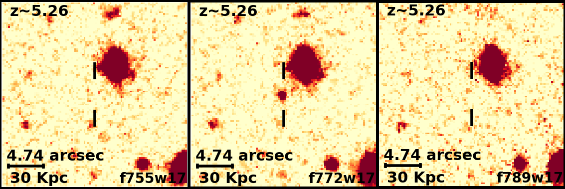
Figure 1: Mosaic of three consecutive SHARDS filters sampling the Ly$\alpha$ emission of the $z\sim 5.26$ pure LAE SHARDS J123720.02+621200.6 (within the vertical marks). The central filter of the image shows the Ly$\alpha$ line in emission. There is no detection at shorter wavelengths, but neither red-ward of the central filter, since the UV continuum is below the SHARDS detection limit. This source shows a weak continuum detection in HST/ACS images red-ward of Ly$\alpha$, though we use the SHARDS images as reference for our definition of pure LAEs. North is up, East is left.

3 Methods

In order to shed light into the nature and evolution of LAEs and LBGs, we have used the Code Investigating GALaxy Emission (cigale, Noll et al., 2009; Boquien et al., 2019). This python software builds stellar populations from synthetic models combined with various Star Formation Histories (SFHs). cigale calculates the emission from gas ionised by massive stars, applying an attenuation law to both the ionised gas and the stars with a differential attenuation between young and old stars. The energy absorbed is re-emitted by the dust at mid/far infrared wavelengths. Combining all the input parameters given, cigale creates a grid of models that are compared with the observed data, checking their likelihood and selecting the best fit for each object. This best-fitting model is then used to derive the main physical parameters. For more details about cigale, we refer to Noll et al. (2009) and Boquien et al. (2019).

3.1 The models

We use the commonly adopted exponentially declining SFH to model our SPs, as in, e.g., Papovich et al. (2001), Pérez-González et al. (2003), Pérez-González et al. (2008), Serra et al. (2011), Rodriguez Espinosa et al. (2014) and Grazian et al. (2015) but see also Carnall et al. (2019) and Leja et al. (2019) for further discussions on SFHs. For this purpose, cigale allows the use of a double exponential SFH consisting in a first decaying exponential corresponding to the long-term star formation responsible of the bulk of stellar mass, plus a second exponential that models recent bursts of star formation. The combined SFHs can be expressed as follows:

$$\mathrm{SFR}(t)\propto\begin{cases}\exp(-t/\tau_{0})&\mbox{if }t<t_{0}-t_{1}\\ \exp(-t/\tau_{0})+k\cdot\exp(-t/\tau_{1})&\mbox{if }t\geq t_{0}-t_{1},\end{cases}$$ (1)

where $\tau_{0}$ and $\tau_{1}$ are the $e$-folding times of the old and young exponential SPs, respectively, and $k$ is a constant indicating the relative strength of the young burst. The time $t_{1}$ is the age of the young population, while $t_{0}$ is so for the old one (see Fig. 2). Furthermore, the fraction of stars formed in the young SP relative to the total stellar mass is given by the burst strength $f$, which can be expressed using discrete integrals, as cigale accounts for the SFH with a period of 1 Myr:

$$f=\frac{k\sum_{t=t_{0}-t_{1}-1}^{t_{0}-1}\exp(-t/\tau_{1})}{\sum_{t=0}^{t_{0}-1}\exp(-t/\tau_{0})+k\sum_{t=t_{0}-t_{1}-1}^{t_{0}-1}\exp(-t/\tau_{1})}.$$ (2)

With this definition, $k$ can be written in the following way:

$$k=\frac{f}{1-f}\cdot\frac{\sum_{t=0}^{t_{0}-1}\exp(-t/\tau_{0})}{\sum_{t=t_{0}-t_{1}-1}^{t_{0}-1}\exp(-t/\tau_{1})},$$ (3)

which indeed leads to the classical case of a single exponential model when $f=0$.

Figure 2: Double exponentially declining SFH for a main SP with different $e$-folding times (different line styles) presenting a second burst of star formation (solid orange line) for an arbitrary $f$ value. $t=0$ corresponds to the formation of the galaxy, while $t_{0}$ (grey dotted vertical line) represents its current age and $t_{1}$ is the time elapsed since the beginning of the second burst of star formation to $t_{0}$.

Using this SFH, the models are computed with the Bruzual & Charlot (2003) stellar emission library, adding nebular templates based on Inoue (2011). A Salpeter (1955) IMF is assumed as well as a Calzetti et al. (2000) dust extinction law. In order to avoid degeneracy and save computational time, we take the next approximations to constrain some of the many possible input physical parameters:

• Regarding $e$-folding times, a first test was made using a wide range of $\tau$ values of up to 1 Gyr, finding that a large majority of sources are better fitted with short $e$-folding times (see Fig. 3). In order to preserve the same nature of the SFH for the entire sample, a $\tau\leq 10$ Myr constrain was adopted in the models, both for $\tau_{0}$ and $\tau_{1}$. Note that this short $\tau$ values are consistent with previous models of high-$z$ galaxies as, e.g., Rodriguez Espinosa et al. (2014) and Hernán-Caballero et al. (2017), where fits prefer low values while allowing $\tau$ to vary. These short $\tau$ values correspond to SPs representing bursts of star formation.

  

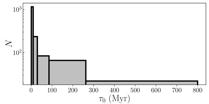
  Figure 3: Distribution of the main SP $e$-folding times of the best-fitting models obtained leaving $\tau$ free up to 1 Gyr. Logarithmic bin widths are used for a better visualisation of the distribution at $\tau\gtrsim 10$ Myr.

• The Ly$\alpha$ escape fraction ($f_{\mathrm{esc}}$) is set to 0.15, consistent with previous calculations at high-$z$ (Robertson et al., 2010; Hayes et al., 2011; Rodriguez Espinosa et al., 2014; Matthee et al., 2016; Sobral et al., 2017, 2018b). Very different escape fraction values are estimated in most recent works. Sobral et al. (2018b) show that the Ly$\alpha$ escape fraction for luminous $z\sim 2$-3 LAEs is very large ($f_{\mathrm{esc}}\sim 0.5$). The Ly$\alpha$ escape fraction for common LAEs at $z=2.23$ is also relatively high according to Sobral et al. (2017), who measured a $f_{\mathrm{esc}}\sim 0.37$ by directly measuring H$\alpha$ and Ly$\alpha$ for these LAEs. On the other side, Matthee et al. (2016) also studied the escape fraction at $z=2.23$ for more massive, star forming and dusty H$\alpha$ emitters, reporting much lower values ($f_{\mathrm{esc}}\sim 0.02-0.05$). The cosmic average of the Ly$\alpha$ escape fraction is estimated around $f_{\mathrm{esc}}\sim 0.05-0.1$ (Hayes et al., 2010; Sobral et al., 2017). Note that the information available in our SEDs does not allow a robust estimation of $f_{\mathrm{esc}}$ for each galaxy and so leaving it as a free parameter would introduce a degeneracy with the age of the young SP. We instead adopt a value of 0.15, which is consistent with the estimation of $f_{\mathrm{esc}}$ through the mean Ly$\alpha$ EW₀ of the sample using the empirical estimator from Sobral & Matthee (2019).

• For the dust correction, the colour excess is assumed to be relatively low, up to $\mathrm{E}(B-V)=0.12$. This agrees with the values of this parameter calculated using the mean $\beta$ slopes, and the $A_{\mathrm{uv}}$ obtained in Arrabal Haro et al. (2018) in the $z$ range of study.

• For the Single Stellar Population (SSP) fits (burst strength of $f=0$), the age is let free within a logarithmic range from 3 to 1500 Myr. On the other hand, the Double Stellar Population (DSP) models have the age of their burst limited to a maximum of 50 Myr, while the age of the underlying population can vary in a logarithmic range from that age to 1500 Myr. Several tests with different age ranges were made to constrain these values. Those carried out with maximum ages below 1500 Myr showed a peak and an abrupt cut at the maximum allowed age, especially at the lowest redshifts. At the same time, no galaxies presented ages above 1500 Myr when the maximum age limit was further extended, which was expected since this value is close to the age of the Universe at our lowest redshift. None of the old SPs from the DSP models were neither younger than 50 Myr when this lower limit was extended.

• The relative strength of the young starburst in the DSP models is limited between a minimum burst strength of $f=0.005$ and a maximum of $f=0.5$, which means that the stellar mass of the young population should represent at least a 0.5% of the total stellar mass of the galaxy in the DSP best fits.

• We allow the metallicity to vary from $Z=10^{-4}$ up to $Z=Z_{\odot}$.

Finally, we make use of a cigale feature that allows us to specify a prior for the integrated Ly$\alpha$ line flux, previously measured in Arrabal Haro et al. (2018). In this way, the Ly$\alpha$ line is weighted more heavily than other data-points. Thereby, we make sure that the Ly$\alpha$ line is well modelled in those galaxies presenting it, avoiding low $\chi^{2}$ solutions where the SED is well fitted except for the filter detecting the line, which otherwise would be selected as best-fitting solutions but that actually do not represent the Ly$\alpha$ emission well. In case of the 1,030 no-Ly$\alpha$ LBGs, to avoid imposing too strong constrains in the non-detected Ly$\alpha$ emission, we provide them with a common negligible input Ly$\alpha$ flux value, while assigning large enough errors to reach the integrated flux of the faintest Ly$\alpha$ line flux measured in the LAEs sample with the SHARDS filters in Arrabal Haro et al. (2018), i.e., $F_{\mathrm{min}}(\mathrm{Ly}\alpha)\simeq 1.3^{+2.0}_{-1.3}\times 10^{-19}\ \mathrm{erg\ s^{-1}\ cm^{-2}}$.

Additionally, in order to explore how the choice of a different dust extinction law affects the main physical parameters derived with the models, we carried out some tests with a randomly selected subsample of 132 sources (preserving the proportion of galaxies from each observational subclass). This subsample was fitted using single SP SFHs with the exact same parameters described in this section but varying from a Calzetti et al. (2000) dust law to a SMC-like dust law. The differences obtained in ages and stellar masses are shown in Fig. 4. It can be appreciated that ages estimated with the Calzetti et al. (2000) extinction law are systematically older. Nonetheless, the age difference is not very significant in terms of the associated error bars of the age estimations.

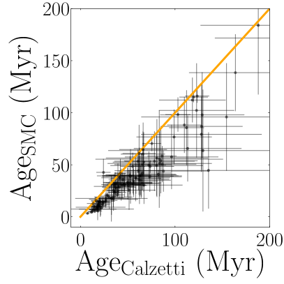
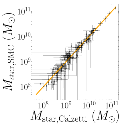
Figure 4: Age and stellar mass differences between a Calzetti and a SMC-like dust extinction law for a random subsample. The one-to-one line is shown in orange. Only ages below 200 Myr are shown for clarity.

The same subsample of 132 objects was also fitted using a larger $f_{\mathrm{esc}}=0.5$. Fig. 5 shows the age and stellar mass differences found. It can be noted that the derived ages are slightly older when using $f_{\mathrm{esc}}=0.15$, especially for the youngest objects, although the age difference is again not relevant if the typical uncertainties of this parameter are taken into account. Moreover, the youngest objects are this time slightly less massive as $f_{\mathrm{esc}}$ increases. This is consistent, since given an observed Ly$\alpha$ flux, it would correspond to a fainter Ly$\alpha$ intrinsic luminosity the higher the $f_{\mathrm{esc}}$ is. The same test was carried out for the entire pure LAEs sample, more prone to have higher $f_{\mathrm{esc}}$ since they present higher Ly$\alpha$ EWs (Sobral & Matthee, 2019). We find the same behaviour. In any case, the stellar masses obtained using different extinction laws and escape fractions are very similar and so no specially significant changes will take place in this regard, even though it is worth noticing that the ages obtained would be shorter if we used the SMC-like dust law and a larger $f_{\mathrm{esc}}$ for the analysis of the entire sample.

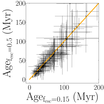
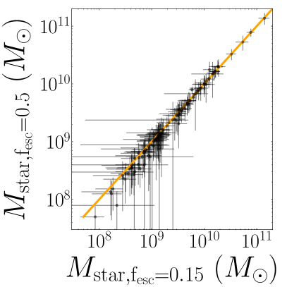
Figure 5: Age and stellar mass differences between $f_{\mathrm{esc}}=0.15$ and $f_{\mathrm{esc}}=0.5$ for a random subsample. The one-to-one line is shown in orange. Only ages below 200 Myr are shown for clarity.

Furthermore, herein we will use an interpretation of the ages in relative terms. This is because of their large uncertainties, especially for the oldest galaxies. Since the existing degeneracy between age and metallicity could be relevant even when relatively comparing the derived ages, another test was made with the 132 random subsample, making several fits fixing a unique metallicity value each time (see Fig. 6). The ages derived show that younger galaxies keep being younger independently of the metallicity. Note that the age-metallicity degeneracy can still be relevant for objects in the edges of the metallicity range employed for the models, although the age differences are within the typically large age errors.

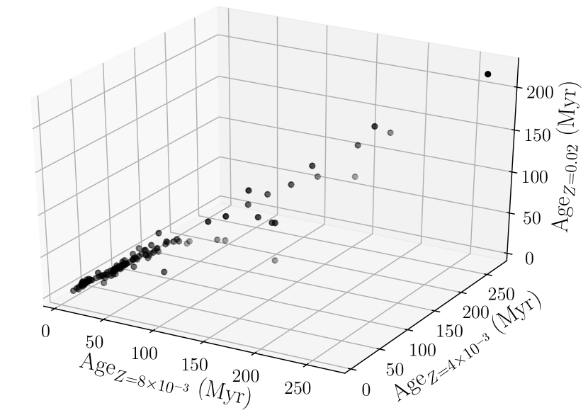
Figure 6: Age comparison of a random subsample for three different fixed metallicities, using three typical values of the general sample. Error bars have been omitted for clarity, but their magnitude is comparable with that in the left panels of Figs. 4 and 5.

3.2 Single and double stellar population considerations

Since we want to determine whether a second SP is needed to model our SHARDS high-$z$ galaxies, both SSP and DSP models are run separately, and their best solutions compared.

To discriminate between the two approaches, we make use of the Bayesian Information Criterion (BIC, Schwarz, 1978) as explained in Liddle (2007) and applied in, e.g., Méndez-Abreu et al. (2018):

$$\mathrm{BIC}=\chi^{2}+q\ln(m),$$ (4)

where $q$ is the number of free parameters of the model used and $m$, the number of independent data points available. In our particular case, SSP models have five free parameters: age, stellar mass, $e$-folding time, colour excess and metallicity. However, $\mathrm{E}(B-V)$ and $Z$ are the same for the young and the old SPs in DSP models, and so those have eight free parameters.

The advantage of using this Bayesian indicator over the $\chi^{2}$ when comparing results from different models is that the BIC penalises the addition of extra free parameters in a stronger way than the normal or even the reduced $\chi^{2}$. Defining the BIC difference between SSP and DSP models as $\Delta\mathrm{BIC}\equiv\mathrm{BIC_{1SP}}-\mathrm{BIC_{2SP}}$, there is a $\Delta\mathrm{BIC}$ threshold from which higher $\Delta\mathrm{BIC}$ values correspond to scenarios where the additional free parameters (in this case, an extra SP) are needed to properly model the galaxy.

To calibrate our $\Delta\mathrm{BIC}$ and obtain the threshold value, a set of theoretical models created with one and two SPs are all fitted with cigale using SSP and DSP models in a separated way in order to compare their $\Delta\mathrm{BIC}$ distributions, following the method used in Méndez-Abreu et al. (2018). In particular, we take the best-fitting SSP model and the best-fitting DSP model of each one of the actual galaxies, convolve them through our photometry filters and use Monte Carlo simulations to create 50 new mock samples by perturbing the convolved photometry with Gaussian noise in accordance with the photometric error of each point. In this way, we obtain $\sim$155,800 mock SEDs whose origin is known (half of them are product of SSP models and the other half come from DSP models). Moreover, these mock SEDs provide a good representation of our observed high-$z$ galaxy sample as they are perturbations of the convolution of the best models fitted to the actual sample. They are then modelled both with single and double SP in order to compare the resulting $\Delta\mathrm{BIC}$ distribution. The obtained histogram of $\Delta\mathrm{BIC}$ values for the mock galaxies is shown in Fig. 7. The limit from which 95.45% (2$\sigma$ significance) of the models come from DSP simulations is given by $\Delta\mathrm{BIC}=-4.50$. Those cases for which $\Delta\mathrm{BIC}>-4.50$ can therefore be selected as our bona fide DSP galaxies. Note that sources with $\Delta\mathrm{BIC}<-4.50$ might still be DSP galaxies. However, we cannot precisely discern the best way of modelling each one of those individual sources in terms of their $\Delta\mathrm{BIC}$, and so the simplest model is favoured over the more complex one. That is, the best SSP fit is taken as the best model for galaxies with $\Delta\mathrm{BIC}<-4.50$, while for those with $\Delta\mathrm{BIC}>-4.50$ the best DSP model is taken. Notice also that the $\Delta\mathrm{BIC}$ value at which the purity of DSP objects reaches the 2$\sigma$ level could vary depending on the proportion of generated SSP and DSP models. In this regard, using a set of Monte Carlo perturbations of both the SSP and DSP best-fitting solution of each original galaxy of the sample is especially relevant to estimate the threshold $\Delta\mathrm{BIC}$ value for this particular sample.

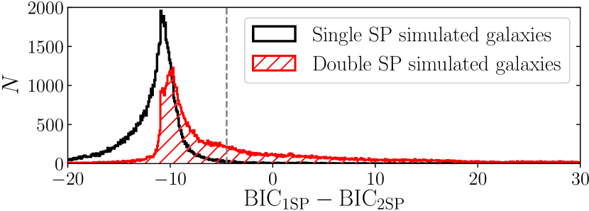
Figure 7: $\Delta\mathrm{BIC}$ distribution of the mock galaxies. The vertical dashed line marks the threshold $\Delta\mathrm{BIC}=-4.50$ beyond which a source requires a DSP model. There is a majority of galaxies for which the SSP and DSP best solutions have similar $\chi^{2}$, resulting in $\Delta\mathrm{BIC}\simeq-10$ for $q_{1}=5$, $q_{2}=8$ at a typical number of independent SED points of $m\sim 30$ (see Eq. 4). For objects with $\Delta\mathrm{BIC}<-4.50$, SSP models are preferred over double ones.

4 Results

With the caveats mentioned in Sec. 3, we obtained good cigale solutions for all the sources in the sample but three very faint ones whose SEDs lack detection in many filters and present large uncertainties in the measurements. In this section we present the results of the model fitting, highlighting the most significant differences found between the three observational classes in our sample. Even though many physical parameters are computed by cigale during the model fitting, we will focus here only in the ages and stellar masses of the sample. We note that there is a well known degeneracy between age, dust and metallicity, and therefore age values should be taken with care in an absolute sense.

In Table 2 we present the IDs, coordinates, ages and stellar masses (split into young and old SP when we select a DSP synthetic spectrum) derived for our 1,555 well modelled galaxies. The median age and $M_{\mathrm{star}}$ of each subgroup are shown in Table 3.

Table 2: Main physical parameters derived from the best models fitted to each source: name of the object using the SHARDS identification, right ascension and declination, photometric redshift, stellar mass, age and $e$-folding time of the main SP and same parameters of the second younger population (when needed). The total $M_{\mathrm{star}}$ is the sum of $M_{\mathrm{star,m}}$ and $M_{\mathrm{star,b}}$. The last three column are left empty when the best solution does not need any additional SP. A full version of this table is available in the on-line version.

Object Name	R.A.	Dec.	$z$	$M_{\mathrm{star,m}}$	$\mathrm{Age_{m}}$	$\tau_{0}$	$M_{\mathrm{star,b}}$	$\mathrm{Age_{b}}$	$\tau_{1}$
	(J2000)	(J2000)		($10^{9}\ M_{\odot}$)	(Myr)	(Myr)	($10^{9}\ M_{\odot}$)	(Myr)	(Myr)
SHARDS20010117	12:35:48.1	62:12:02.4	$4.28\pm 0.06$	$1.88\pm 1.24$	$77\pm 44$	$3.4\pm 2.7$	-	-	-
SHARDS20007539	12:35:48.1	62:12:03.8	$5.38\pm 0.07$	$2.34\pm 1.04$	$24\pm 12$	$4.24\pm 2.35$	-	-	-
SHARDS20012481	12:35:50.9	62:11:58.5	$5.69\pm 0.06$	$2.74\pm 1.51$	$63\pm 31$	$2.91\pm 2.32$	-	-	-
SHARDS20005927	12:35:51.5	62:12:16.5	$3.22\pm 0.07$	$2.8\pm 0.5$	$47\pm 10$	$2.36\pm 1.51$	-	-	-
SHARDS20005405	12:35:51.6	62:12:12.7	$4.03\pm 0.07$	$6.5\pm 1.31$	$74\pm 21$	$2.92\pm 2.2$	-	-	-
SHARDS20008074	12:35:52.2	62:11:20.8	$5.53\pm 0.07$	$0.60\pm 0.32$	$20\pm 9$	$1.9\pm 1.56$	-	-	-
SHARDS20008444	12:35:53.2	62:10:32.9	$4.01\pm 0.07$	$6.3\pm 5.0$	$950\pm 500$	$5.0\pm 3.2$	$0.89\pm 1.30$	$35\pm 12$	$2.02\pm 1.5$
SHARDS20010810	12:35:53.4	62:10:23.3	$5.12\pm 0.06$	$1.4\pm 0.9$	$72\pm 44$	$3.3\pm 2.7$	-	-	-
SHARDS20005669	12:35:54.1	62:10:32.9	$3.36\pm 0.07$	$11.0\pm 7.0$	$357\pm 244$	$5.2\pm 3.3$	$0.46\pm 0.94$	$24\pm 14$	$3.0\pm 2.9$
SHARDS20011405	12:35:54.3	62:10:18.8	$5.37\pm 0.07$	$3.69\pm 1.44$	$80\pm 38$	$3.6\pm 2.7$	-	-	-
SHARDS20006420	12:35:54.4	62:10:33.8	$3.88\pm 0.06$	$7.06\pm 2.49$	$110\pm 50$	$4.3\pm 3.0$	-	-	-
SHARDS20006258	12:35:54.5	62:12:14.6	$3.48\pm 0.06$	$1.1\pm 0.6$	$17\pm 11$	$2.04\pm 1.78$	-	-	-
SHARDS20013727	12:35:55.0	62:12:04.8	$5.96\pm 0.07$	$20.0\pm 10.0$	$294\pm 190$	$5.2\pm 3.3$	$1.12\pm 2.08$	$32\pm 15$	$4.8\pm 3.3$
SHARDS20009009	12:35:55.2	62:11:25.4	$3.89\pm 0.06$	$1.7\pm 0.6$	$66\pm 28$	$3.2\pm 2.48$	-	-	-
SHARDS20006827	12:35:55.7	62:10:19.0	$4.28\pm 0.06$	$1.9\pm 0.8$	$38\pm 16$	$1.83\pm 1.21$	-	-	-
…	…	…	…	…	…	…	…	…	…

Table 3: Median age and stellar mass for each group and subgroup in the sample. Ages shown correspond to the age of the old SP. Error bars correspond to the standard deviation of the median.

Type	Age (Myr)	$M_{\mathrm{star}}$ ($10^{9}\ M_{\odot}$)
No-Ly$\alpha$ LBGs	$71\pm 12$	$3.5\pm 1.1$
LAE-LBGs	$40\pm 27$	$2.3\pm 1.7$
Pure LAEs	$26^{+41}_{-25}$	$0.56^{+1.20}_{-0.55}$

Additionally, as previously discussed in Sec. 2, the availability of IRAC detection in the SEDs is especially relevant to discern whether we need to add a second SP or not, as well as to reliably constrain the main physical parameters derived. In Table 4 we give an overview of the proportion of objects within each subfamily with detection in IRAC as well as the fraction of sources requiring the addition of a second SP. Indeed, $\sim$98% of the DSP galaxies are detected in IRAC. Moreover, these sources present median age and $M_{\mathrm{star}}$ relative errors of 40% and 33%, respectively, while these relative errors increase to 53% and 58% for the age and $M_{\mathrm{star}}$ of the IRAC-undetected objects.

Table 4: Number and fraction of objects from each family detected in IRAC and number of sources requiring two SPs to model their SEDs according to the $\Delta\mathrm{BIC}$ criterion.

Type	$N_{\mathrm{total}}$	$N_{\mathrm{IRAC}}$	$N_{\mathrm{DSP}}$
No-Ly$\alpha$ LBGs	1030	882 (86%)	164 (15.9%)
LAE-LBGs	404	347 (86%)	135 (33.4%)
Pure LAEs	124	71 (57%)	27 (21.8%)

4.1 Stellar populations required

We apply the calibrated $\Delta\mathrm{BIC}$ criterion explained in Sec. 3.2 to get the best-fitting model for each individual galaxy of the sample with either one or two SPs, finding that in most cases (79.0%), these high-$z$ galaxies do not require the addition of an extra SP to model their SEDs. The frequency distribution of $\Delta\mathrm{BIC}$ for the three families is shown in Fig. 8. Even though the three groups clearly present their peaks within the SSP $\Delta\mathrm{BIC}$ range, it is worth noticing that the LAE-LBGs family is wider and the one that more likely tends towards higher $\Delta\mathrm{BIC}$ values. Specifically, only 15.9% and 21.8% of the no-Ly$\alpha$ LBGs and pure LAEs need of a second SP in their fits, respectively, while this occurs for 33.4% of the LAE-LBGs (see Table 4). Further discussion on the reasons of this behaviour will be given in next subsections and Sec. 5.

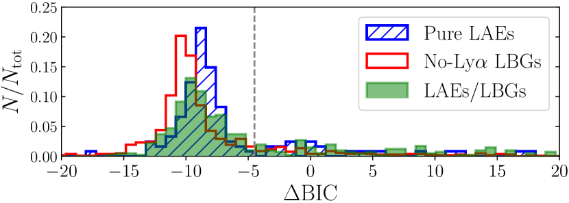
Figure 8: $\Delta\mathrm{BIC}$ distribution of pure LAEs (blue diagonals), LBGs with no Ly$\alpha$ emission line (red unfilled) and LAE-LBGs (solid green) weighted by the amount of objects within each class. The $\Delta\mathrm{BIC}=-4.50$ value from which two SPs are needed is depicted by a vertical dashed line. It can be appreciated that the majority of objects (79.0%) are well modelled using a SSP model. Thus, pure LAEs and no-Ly$\alpha$ LBGs are proportionally less represented in the DSP models $\Delta\mathrm{BIC}$ range than LAE-LBGs, whose distribution is wider and more extended towards high $\Delta\mathrm{BIC}$ values.

4.2 Age differences

Looking at the age distribution in Fig. 9, a large difference can be appreciated between pure LAEs and no-Ly$\alpha$ LBGs, where the first ones are much younger, with a median age of $26^{+41}_{-25}$ Myr, while that of the no-Ly$\alpha$ LBGs is $71\pm 12$ Myr. It can also be appreciated a clear dichotomy in the age distribution led by SSP and DSP models. This dichotomy is indeed product of the use of burst-like SFHs joined to the large uncertainties associated to the physical parameters of the old SP in DSP models. In the cases where two SPs are needed to reproduce the SED, the Ly alpha line and UV continuum are well fitted by the young and well defined SP and so the old SP can adopt a large variety of ages in order to fit the continuum points at longer wavelengths. When this happens, very large ages typically lead to the best $\chi^{2}$ of the global fit, producing a not representative gap of sources at intermediate ages. The discussion in this work is however focused on the relative differences between SSP and DSP sources, but the exact values of the age for the DSP models are too uncertain to consider them as accurate absolute calculations, but only as an estimation of the order of magnitude.

Even though the age dichotomy is found for the three families, special attention is put onto the LAE-LBGs as their SEDs present emission features better constraining the young and old SP and therefore the need of a DSP model: Ly$\alpha$ emission line (not present in no-Ly$\alpha$ LBGs) and bright continuum measure, especially relevant at long wavelengths (not present in pure LAEs). Moreover, this subgroup is the one that more frequently needs the use of DSP models. The two peaks of the LAE-LBGs age distribution can be associated to the inherent nature of the models fitting those objects, split into: 1) SSP LAE-LBGs, corresponding to very young galaxies (median age $\sim 27$ Myr) with large enough $M_{\mathrm{star}}$ to show a prominent UV continuum detectable in SHARDS, and 2) DSP LAE-LBGs, representing a more evolved galaxy with an older underlying massive SP suffering a recent star-forming episode, thus the additional young SP.

To shed light on whether the SSP age difference between no-Ly$\alpha$ LBGs and LAE-LBGs is only driven by the detection of the Ly$\alpha$ line or not, SSP LAE-LBGs are fitted a second time omitting the Ly$\alpha$ line contribution from their SEDs by replacing the flux in the filter sampling the Ly$\alpha$ line with an estimation of the continuum emission from the adjacent SHARDS filters or the broad band HST/ACS photometry when needed. The new Ly$\alpha$-removed photometry is then refitted with and without the integrated Ly$\alpha$ flux prior used for the no-Ly$\alpha$ LBGs (see Sec. 3.1). In both cases, the median age obtained for the SSP LAE-LBGs in this second run is only $\sim 6$-8 Myr younger than that of the SSP no-Ly$\alpha$ LBGs, being not different within their errors. This highlights that the youthfulness of the SSP LAE-LBGs in the models comes from the Ly$\alpha$ emission line, also implying that some no-Ly$\alpha$ LBGs for which the intrinsic Ly$\alpha$ line remains undetected because of scattering or dust extinction could be equally young as well, adding an extra difficulty in the characterisation of this last subgroup.

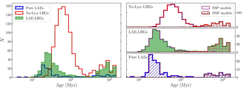
Figure 9: Left panel: Main SP age distribution for the pure LAEs (blue diagonals), LAE-LBGs (solid green) and no Ly$\alpha$ line LBGs (unfilled red). Notice that most pure LAEs show low ages (71% below 50 Myr), while the no-Ly$\alpha$ LBGs are typically older, peaking at $\sim 71$ Myr. Right panels: Split contribution of SSP and DSP models to the age distribution of each family. The observed dichotomy is due to the use of burst-like SFHs joined to the limitations of the SEDs to constrain the old SP in DSP models.

4.3 Stellar mass differences

Regarding the stellar mass, the distribution presented in Fig. 10 shows again a clear difference between pure LAEs (median $M_{\mathrm{star}}\sim 5.6^{+12.0}_{-5.5}\times 10^{8}\ M_{\odot}$) and no-Ly$\alpha$ LBGs (median $M_{\mathrm{star}}\sim 3.5\pm 1.1\times 10^{9}\ M_{\odot}$), with $M_{\mathrm{star}}$ an order of magnitude higher for the latter ones. Notice also that the LAE-LBGs present a smooth $M_{\mathrm{star}}$ distribution along a wider $M_{\mathrm{star}}$ range, with a median value of $2.3\pm 1.7\times 10^{9}\ M_{\odot}$. Here again, when we separate the contribution of SSP and DSP models, it can be appreciated that the more massive side of the $M_{\mathrm{star}}$ distribution is driven by the DSP sources while the low side of the mass distribution corresponds to the SSP ones. This result is not surprising once we take into account that, according with Fig. 9, the DSP galaxies are much older and therefore have typically been forming stars for a much longer time, becoming more massive on average. Additionally, the detection of a relevant second SP is only possible in the most massive galaxies, where the old population presents a strong enough brightness at the longest wavelengths. In the particular case of the LAE-LBGs, these DSP objects could be understood as no-Ly$\alpha$ LBGs that see their star formation increased by some triggering physical mechanism (mergers or neighbour gravitational interaction, instabilities, large cosmic web gas accretion, etc.) becoming LAE-LBGs (see Fig. 17).

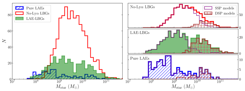
Figure 10: Left panel: Stellar mass distribution of pure LAEs (blue diagonals), LAE-LBGs (solid green) and no-Ly$\alpha$ LBGs (unfilled red). Notice that both LBGs families show substantially higher $M_{\mathrm{star}}$ than the pure LAEs. Right panels: Split contribution of SSP and DSP models to the age distribution of each family. It can also be appreciated that the DSP galaxies present the larger stellar masses.

4.4 Burst strength

For the 326 galaxies better fitted using DSP models, a study of the relevance of each population in terms of mass is done by looking at the burst strength parameter $f$, whose distribution is shown in Fig. 11. We find that the burst strength remains low in almost all cases, with a 96% of the objects at $f<0.17$. This distribution shows that even in the cases where a DSP modelling gives better results, these galaxies are still dominated by the main old SP in terms of stellar mass. Furthermore, the $M_{\mathrm{star}}$ of the young SP is almost negligible. However, it is important to highlight that the relevance of this young population comes with the conspicuous Ly$\alpha$ emission line and UV luminosity, which could not be reproduced using only a single old SP. No significant differences of the burst strength distribution were noticed among the three observational subgroups and no trend with redshift was neither found.

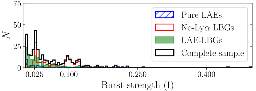
Figure 11: Distribution of the burst strength in the sources better approached by DSP models. The higher frequencies at low burst strength value indicate that even though two SPs are needed to properly model these objects, their SEDs are mostly the product of a main massive dominant old SP, with the young SP being almost irrelevant if not for the UV luminosity.

4.5 Stellar mass functions

With the stellar masses derived from the best-fitting SP models we build Stellar Mass Functions (SMFs) at each redshift up to our stellar mass completeness. To estimate this completeness $M_{\mathrm{star},\mathrm{lim}}$, we make use of the technique employed in e.g., Pozzetti et al. (2010) and Davidzon et al. (2017) to calculate the stellar mass limit for a survey limited in magnitude. This method consists on taking the masses derived in each redshift bin and rescaling them to the magnitude limit of our survey:

$$\log(M_{*,\mathrm{resc}})=\log(M_{\mathrm{star}})+0.4(m-m_{\mathrm{lim}}).$$ (5)

We adopt $m_{\mathrm{lim}}\sim 27$ AB as an approximation of the average 3$\sigma$ limit detection in the SHARDS filters. The $M_{\mathrm{star},\mathrm{lim}}$ is then defined as the 90th percentile of the $M_{\mathrm{star},\mathrm{resc}}$ distribution. With this method, we estimate an average $M_{\mathrm{star},\mathrm{lim}}\sim 7.4\times 10^{9}\ M_{\odot}$ for our stellar mass sample. This $M_{\mathrm{star}}$ completeness means that our SMFs are dominated by the LBGs population, as the majority of pure LAEs present masses below that limit (see Fig. 10). Additionally, a $V_{\mathrm{max}}$ correction (Schmidt, 1968) is considered when building our SMFs. The main advantage of the $V_{\mathrm{max}}$ correction is that it directly provides the normalisation of the SMF. To model the SMF, we make use of the widely used Schechter (1976) function:

$$\phi(M)dM=\phi^{*}\exp(-M/M^{*})(M/M^{*})^{\alpha}dM/M^{*},$$ (6)

which can be better expressed in the $\log M$ space when working with SMFs:

$$\phi(M)d\log M=\phi^{*}\ln 10\exp(-10^{\log M-\log M^{*}})$$

$$\times\ (10^{\log M-\log M^{*}})^{\alpha+1}d\log M.$$ (7)

The resulting SMFs are shown in Fig. 12 as well as the best Schechter fits and their $1\sigma$ and $3\sigma$ confidence intervals derived from Monte Carlo simulations perturbing the points themselves as well as the $M_{\mathrm{star}}$ bin sizes and centres, as explained in more detail in appendix A. The error bars of our points correspond to the Poissonian uncertainties. The few points available at $z\sim 5$-6 up to our stellar mass completeness make the estimation of the $\alpha$ slope very difficult at these $z$, hence the large uncertainties derived from the fitting. Moreover, the calculated $M_{\mathrm{star},\mathrm{lim}}\sim 8.3\times 10^{9}\ M_{\odot}$ at $z\sim 6$ seems to be slightly underestimated as it includes incomplete SMF points close to the $M^{*}$ knee for certain perturbations of the $M_{\mathrm{star}}$ bins, which derive in positive $\alpha$ values. To avoid this issue, we constrain the $\alpha$ fitting to $-3.0<\alpha<-0.9$ at $z\sim 6$ and limit the SMF points to those strictly increasing up to our $M_{\mathrm{star},\mathrm{lim}}$ as we consider that further ones are actually incomplete. Note that this approach could be slightly biasing the obtained $\alpha$ values towards more negative values at $z\sim 6$. More details on the fitting process, as well as the significance contours of the fitted Schechter parameters at each redshift are given in appendix A.

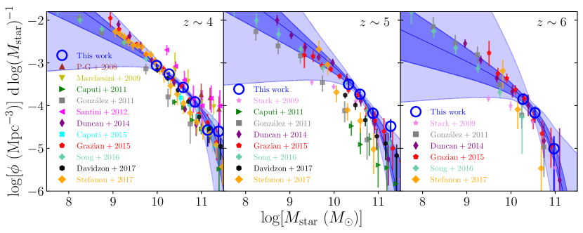
Figure 12: SMF at $z\sim 4$, $z\sim 5$ and $z\sim 6$. The Monte Carlo best fit is indicated with the solid blue line, while the darker and lighter blue contours correspond to the 68% and 99.7% confidence intervals, respectively. For comparison, we also show previous SMF calculations from Pérez-González et al. (2008) ($3.5<z<4.0$), Marchesini et al. (2009) ($3.0<z<4.0$), Stark et al. (2009), Caputi et al. (2011), González et al. (2011), Santini et al. (2012), Duncan et al. (2014), Caputi et al. (2015), Grazian et al. (2015), Song et al. (2016), Davidzon et al. (2017) and Stefanon et al. (2017). All SMFs have been rescaled to a Salpeter IMF for comparison.

By integrating the SMF from $10^{8}$ to $10^{13}$ $M_{\odot}$ (as in, e.g., Duncan et al., 2014; Grazian et al., 2015; Song et al., 2016), we obtain the Stellar Mass Density (SMD) at each redshift. The best-fitting Schechter parameters are summarised in Table 5 as well as the calculated SMDs. A comparison of our SMD estimations with previous works is shown in Fig. 13, where it can be appreciated that our calculations follow the general trend with $z$ reported by previous authors, presenting a especially large uncertainty at $z\sim 5$-6 due to the mentioned lack of information in the low mass regime of our SMF at that redshift and the corresponding uncertainty of the estimated $\alpha$ slope.

Table 5: SMF best-fitting Schechter parameters and the corresponding SMD obtained by integration of the SMF from $10^{8}$ to $10^{13}$ $M_{\odot}$. The shown uncertainties correspond to 1$\sigma$ significance. The redshift ranges represented correspond to $3.5\leq z<4.5$; $4.5\leq z<5.5$ and $5.5\leq z<6.5$, respectively.

$\langle z\rangle$	$\log M^{*}$	$\log\phi^{*}$	$\alpha$	$\log\rho_{*}$
$4$	$11.06^{+0.33}_{-0.27}$	$-4.14^{+0.39}_{-0.45}$	$-1.72^{+0.24}_{-0.14}$	$7.36^{+0.08}_{-0.10}$
$5$	$10.78^{+0.53}_{-0.07}$	$-3.97^{+0.10}_{-0.79}$	$-1.76^{+0.19}_{-0.26}$	$7.26^{+0.20}_{-0.15}$
$6$	$10.51^{+0.08}_{-0.03}$	$-4.06^{+0.02}_{-0.06}$	$-1.49^{+0.22}_{-0.21}$	$6.70^{+0.14}_{-0.19}$

Figure 13: SMD obtained by integration of the SMFs at each $z$. To give a global view of the SMD evolution with $z$, we show previous estimations from Dickinson et al. (2003, D03), Fontana et al. (2006, F06), Pozzetti et al. (2007, P07), Pérez-González et al. (2008, PG08), Kajisawa et al. (2009, K09), Marchesini et al. (2009, M09), Marchesini et al. (2010, M10), Labbé et al. (2010, L10), Caputi et al. (2011, C11), González et al. (2011, G11), Mortlock et al. (2011, M11), Lee et al. (2012, L12), Santini et al. (2012, S12), Ilbert et al. (2013, I13), Muzzin et al. (2013, M13), Duncan et al. (2014, D14), Tomczak et al. (2014, T14), Grazian et al. (2015, G15), Song et al. (2016, S16) and Davidzon et al. (2017, D17). All SMDs are rescaled to a Salpeter IMF.

4.6 SFR-$\boldsymbol{M_{\mathrm{star}}}$ relation

To build SFR-$M_{\mathrm{star}}$ relations at each $z$ and compare them with previous estimations, we make use of the SFRs calculated for this sample in Arrabal Haro et al. (2018) using the Kennicutt (1998) and Madau et al. (1998) prescriptions after correcting for both galactic and internal dust extinction following Schlafly & Finkbeiner (2011) and Calzetti et al. (2000), respectively. Those SFRs were calculated using the Ly$\alpha$ emission line for the pure LAEs and the UV luminosity for the LBGs. The SFRs of the pure LAEs are estimated through their Ly$\alpha$ luminosity in Arrabal Haro et al. (2018), thus they are not on equal terms with the UV-derived SFR-$M_{\mathrm{star}}$ relation. To avoid using multiple different SFR indicators, we only make use of the SFRs estimated through $L_{1500}$, which allow us to compare our results with previous works studying this relation in a similar fashion such as, e.g, Salmon et al. (2015). Moreover, the SFRs derived through the Ly$\alpha$ line luminosity can be strongly affected by resonant scattering. For a recent detailed study of the SFR-$M_{\mathrm{star}}$ relation estimating SFRs of high-$z$ LAEs through their Ly$\alpha$ luminosity, see, e.g., Santos et al. (2020). The so-called SFR-$M_{\mathrm{star}}$ main sequence (Fig. 14) is modelled using the common linear approach between the logarithm of these magnitudes (e.g., Salmon et al., 2015):

$$\log[\mathrm{SFR}\ (M_{\odot}\ \mathrm{yr^{-1}})]=\beta\log[M_{\mathrm{star}}\ (M_{\odot})]+C.$$ (8)

Figure 14: SFR-$M_{\mathrm{star}}$ relation measured at each redshift using the UV-derived SFRs. Pure LAEs are not considered in this SFR-$M_{\mathrm{star}}$ relation, since their SFRs are only estimated through their Ly$\alpha$ luminosity. The error bars of our data (blue circles) is associated to the standard error of the median SFR at each $M_{\mathrm{star}}$ bin. The blue solid line corresponds to the best fit and the darker and lighter blue regions delimit the 1$\sigma$ and 3$\sigma$ confidence intervals of the fit, respectively. Theoretical predictions from Behroozi et al. (2013, faded green contour) and Davé et al. (2013, faded yellow contour) show slightly steeper slopes than the observations from Salmon et al. (2015) and our sample. The slope of the SFR-$M_{\mathrm{star}}$ relation does not show a significant change with $z$.

The error bars shown in Fig. 14 correspond to the standard error of the median SFR at each $M_{\mathrm{star}}$ bin. To fit the slope and zero point of the relation we applied Monte Carlo methods not only perturbing the points within the errors, but also the $M_{\mathrm{star}}$ bin centres and sizes in a range of 0.1-0.5 dex. To compare our results, we use data from semi-empirical models (Behroozi et al., 2013), hydrodynamic simulations (Davé et al., 2013) and observational data from Salmon et al. (2015). Note that the distribution of these observational data matches very well ours, though the trend of the theoretical models is slightly steeper. The best-fitted values of $\beta$ and $C$ are given in Table 6. It can be noticed that the slope of the SFR-$M_{\mathrm{star}}$ remains invariable with $z$ within errors, as it has been previously reported in the literature (Stark et al., 2009; González et al., 2010; Papovich et al., 2011; Salmon et al., 2015). The implications of this absence of evolution in the SFR-$M_{\mathrm{star}}$ relation with $z$ will be further discussed in Sec 5.

In order to study the distribution of the different subclasses along this main sequence employing the same SFR estimator for all of them, we make use of the main sequence built up with the SFRs derived from the best-fitting SSP cigale models (Fig. 15). Note that the different nature of the SFR estimators makes their absolute values difficult to compare as they can differ substantially. Indeed, as reported in, e.g., Otí-Floranes & Mas-Hesse (2010), usual SFR estimators tend to have strong assumptions on the SFH. These assumptions can be incorrect when using burst-like SFHs as the ones employed for high-$z$ galaxies in this paper, resulting in very differing SFR estimations. Because of this, the absolute model-derived SFRs from burst-like SPs are higher than those from Behroozi et al. (2013) and Davé et al. (2013), who did not employ short-lived star formation episodes. Nevertheless, their main sequence slope is similar to the model-derived slope obtained for our sample. For more details on differences in SFR calculation, see Boquien et al. (2014) or Boquien et al. (2016), among others. The reason to study the SFR-$M_{\mathrm{star}}$ using the SFRs from the models is, apart from having an additional measure of the main sequence slope, to analyse relative differences between subclasses from a common SFR estimation. The best-fitting parameters of this model-derived SFR-$M_{\mathrm{star}}$ relation are also shown in Table 6. The slope obtained in this second case is slightly steeper than those obtained employing the UV-derived SFRs, getting closer to the theoretically predicted by Behroozi et al. (2013) and Davé et al. (2013). Furthermore, the SFR-$M_{\mathrm{star}}$ relation derived from the best-fitting SSP models also remains constant between $z=4$-6, reinforcing this result.

Regarding the different subgroups distribution, it can be appreciated that pure LAEs occupy the left end of the main sequence, corresponding to lower stellar masses and SFRs, while LBGs conform the bulk at intermediate and large masses. Note that both LAE-LBGs and pure LAEs appear in the upper side of the main sequence, in agreement with the idea of these sources experimenting a recent star-forming episode, while no-Ly$\alpha$ LBGs are placed in the bottom-middle side of it.

Table 6: Best-fitting parameters for the SFR-$M_{\mathrm{star}}$ main sequence built up using UV-derived SFRs (second and third columns) and model-derived SFRs (last two columns).

$\langle z\rangle$	$\beta_{L_{1500}}$	$C_{L_{1500}}$	$\beta_{\mathrm{mod}}$	$C_{\mathrm{mod}}$
$4$	$0.48^{+0.07}_{-0.10}$	$-3.45^{+0.92}_{-0.70}$	$0.83^{+0.09}_{-0.06}$	$-6.01^{+0.52}_{-0.76}$
$5$	$0.46^{+0.12}_{-0.10}$	$-3.25^{+0.91}_{-1.13}$	$0.79^{+0.10}_{-0.11}$	$-5.56^{+0.92}_{-0.97}$
$6$	$0.51^{+0.26}_{-0.19}$	$-3.56^{+1.80}_{-2.52}$	$0.82^{+0.15}_{-0.16}$	$-5.89^{+1.42}_{-1.43}$

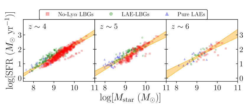
Figure 15: SFR-$M_{\mathrm{star}}$ main sequence measured at each redshift using the SFRs given by the best-fitting SSP cigale models. The orange region delimit the 3$\sigma$ confidence interval of the fit. The slope of the SFR-$M_{\mathrm{star}}$ relation does not change with $z$ within our redshift range.

5 Discussion

One of the particularities of this study lays on the very short $\tau$ values found for the best-fitting models of the sample. These short $\tau$ values represents bursts of star formation. This result leads to younger ages than those typically obtained in previous models of high-$z$ LAEs and LBGs using fairly constant SFHs, where the estimate ages are of the order of few hundreds Myr (see, e.g, Dayal & Ferrara, 2012). However, shorter ages like the ones presented here for SSP star-forming sources have also been obtained for LAEs and LBGs using different SFHs. Jiang et al. (2016), for example, found a similar age bimodality (also present in their $M_{\mathrm{star}}$ distribution) when modelling high-$z$ galaxies with exponentially declining SFHs with larger $e$-folding time ($\tau$=200 Myr) and smoothly raising SFHs. Employing a constant SFH, Yuma et al. (2010) also found very short ages (median age of 25 Myr) for $z\sim 5$ LAEs. In any case, the age estimation of high-$z$ LAEs and LBGs through SED fitting presents large uncertainties independently of the input parameters of the models employed, and so our interest is in spotting relative differences between observational subfamilies rather than calculate exact absolute age values.

The stellar masses found for high-$z$ LAEs and LBGs are better constrained in the literature, presenting values in the 10⁸-10¹¹ $M_{\odot}$ range with median values of a few $10^{9}$ $M_{\odot}$ (see, e.g, Yuma et al., 2010; Dayal & Ferrara, 2012; Duncan et al., 2014; Grazian et al., 2015; Jiang et al., 2016; Song et al., 2016; Davidzon et al., 2017), with LAEs typically presenting lower masses, which can also be related with a selection bias effect as stated in Dayal & Ferrara (2012). The stellar masses found in this work are in good agreement with previous estimations at high redshifts.

5.1 LAEs and LBGs stellar population differences

From the ages and stellar masses derived with cigale we can build some relations between the different observational families previously defined. As highlighted in Sec. 4, the age values are on the low side due to the existing degeneracy between dust extinction, metallicity and the age itself, and so these absolute values should be taken with care. Nevertheless, we can use them to trace age differences between our various families of LAEs and LBGs.

On the one side, we have the pure LAEs, defined as objects with strong Ly$\alpha$ line emission but a faint UV continuum ($m_{1500}\gtrsim 27$ AB). These sources typically present low stellar masses in their young SP (median $M_{\mathrm{star}}=5.6^{+12.0}_{-5.5}\times 10^{8}\ M_{\odot}$). Additionally, the presence of strong Ly$\alpha$ emission quickly decays with time as it traces the Lyman continuum radiation which is only produced by O and late type B stars with $M>10\ M_{\odot}$ and lifetimes of a few Myr, and so it is an indicator of recent star formation. That, on top of the low $M_{\mathrm{star}}$, indicates that these galaxies should be typically young, since they are currently in a star-forming burst but have not been forming stars long enough, in the past, to present larger stellar masses. This hypothesis is confirmed by the median age obtained with the cigale fitting for this family ($26^{+41}_{-25}$ Myr). According to this, many of these sources could indeed be experimenting one of their first episodes of star formation, or at least one strong enough to overtake all the older stars in luminosity. Furthermore, we also find that most of these objects can be explained using a single decaying exponential SFH. An example of this is shown in Fig. 16, where the Ly$\alpha$ emission line, together with the absence of strong UV continuum photometric points makes it possible to model these pure LAEs in terms of a single young and low mass SP. Note that some of these SSP-fitted sources could actually host an old SP from previous star-forming episodes. However, these old SPs are not massive enough to be identified over the young SP luminosity. The 27 DSP pure LAEs found in this work can be modelled as older and more massive galaxies that are experimenting a recent star-forming episode. This recent star formation is not strong enough to raise the UV continuum up to a flux level measurable in SHARDS, but it does raise the Ly$\alpha$ emission associated to young short-living stars, while the old SP makes them detectable at longer wavelengths in the IRAC range.

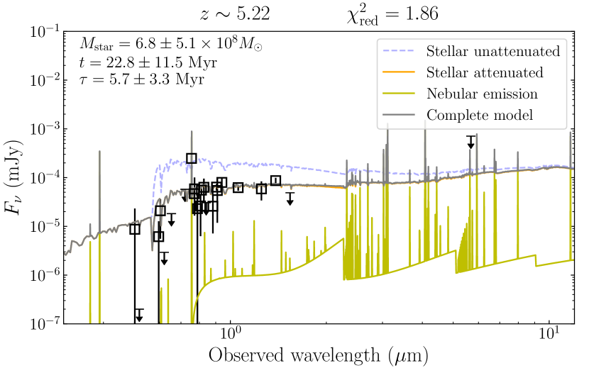
Figure 16: Best model for the pure LAE SHARDS J123640.20+621228.8. The black squares are the photometric points used in the fit. The final model (grey line) is split into the attenuated stellar emission (orange line) and the nebular emission (yellow line). The non-attenuated stellar emission is also represented by the dashed bluish line. The SED presents a clear Ly$\alpha$ emission line, but the absence of strong continuum points at the longest sampled wavelengths makes it possible to fit it with a single young and not so massive SP.

For the LAE-LBGs, the dichotomy found in their age and $M_{\mathrm{star}}$ distributions shown in the right panels of Figs. 9 and 10 set a similar differentiation between SSP LAE-LBGs and DSP LAE-LBGs as with pure LAEs. The objects of this family that can be fitted using a SSP are the youngest and less massive within the LAE-LBGs. These cases do not present any strong emission at longer wavelengths and can therefore be reproduced by a young SP (median age of $27\pm 6$ Myr) with Ly$\alpha$ line in emission and a fairly flat UV continuum. According to the description given in the previous paragraph for the pure LAEs, the SSP LAE-LBGs would just be the most massive members of that same class: young galaxies well modelled by a SSP, with the only difference that SSP LAE-LBGs present a massive enough young SP (median $M_{\mathrm{star}}=1.04\pm 0.48\times 10^{9}\ M_{\odot}$) to show an UV continuum detectable in SHARDS, preventing the pure LAEs observational classification but actually belonging to the same kind of objects. On the other side, the DSP LAE-LBGs are much older and more massive. The need of a second SP to understand the SEDs of this subgroup comes from the presence of the Ly$\alpha$ emission line plus some bright IRAC points. Both emission features cannot be simultaneously fitted by a SSP with the characteristics employed in this work (as in, e.g., Rodriguez Espinosa et al., 2014). In Fig. 17, we present two examples to illustrate what happens when we try to fit some of these objects SEDs with a SSP that either fits well the Ly$\alpha$ line but not the longer wavelength continuum or the other way around. The cigale best solutions for this subgroup suggest that the DSP LAE-LBGs can be understood as older galaxies with an old SP that raises the continuum emission at longer wavelengths, currently experimenting a recent star-forming episode triggered by accretion of new gas or by mergers. It makes sense thinking about the observational definition of pure LAEs and LAE-LBGs being the same kind of galaxies (just LAEs) with the only difference that pure LAEs are more frequently fitted by SSP models, while LAE-LBGs require the addition of the old SP more often.

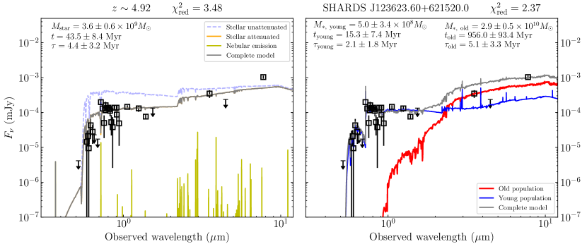
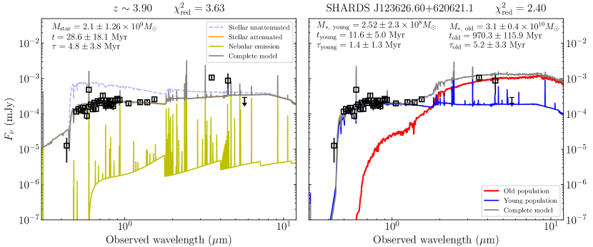
Figure 17: Best SSP and DSP solutions for two LAE-LBGs modelled each with two SPs. The objects SHARDS J123623.60+621520.0 and SHARDS J123626.60+620621.1 are shown in the upper and lower panels, respectively. In each case, the left frame shows the best SSP fit. The black squares are the photometric points of the SED, the yellow line shows the nebular emission, the stellar attenuated emission is represented in orange and the stellar non-attenuated emission is plotted with a dashed bluish line. The grey line shows the complete model. On the other side, the right frames correspond to the best DSP fits, where the different components of the emission have been omitted for clarity and the contributions of the old and young SPs are represented in red and blue, respectively. For the upper source, the best SSP model matches relatively well the continuum but is not able to reproduce the Ly$\alpha$ emission line detected. The addition of a second SP becomes necessary to not only to match that Ly$\alpha$ emission, but even to improve the continuum fit in the IRAC range. The opposite scenario can be seen in the lower source, where the best SSP fit manages to reproduce the line emission at the cost of leaving the reddest points unfitted. This time, the second population added is an old one that contributes to raise the continuum emission in the IRAC range.

On the other side, we have the no-Ly$\alpha$ LBGs, understood as galaxies selected through their Lyman break in the UV continuum emission, but without Ly$\alpha$ line detected in the SHARDS photometry ($F(\mathrm{Ly}\alpha)\lesssim 1.3^{+2.0}_{-1.3}\times 10^{-19}\ \mathrm{erg\ cm^{-2}}$). This family is the oldest and most massive of the SSP models of the three predefined observational families, with a median stellar mass almost an entire order of magnitude above that of the pure LAEs ($M_{\mathrm{star}}=3.5\pm 1.1\times 10^{9}\ M_{\odot}$). The absence of a detectable Ly$\alpha$ line should not be taken as a secure indicator of the relative faintness of the most recent star formation in these objects, since the real Ly$\alpha$ emission of the galaxy can be strongly affected by dust extinction and resonant scattering through the interstellar medium. Indeed, dust extinction affects strongly both the Ly$\alpha$ line and the rest-frame UV continuum. Hence, there is an intrinsic selection effect towards galaxies with low internal extinction. Ly$\alpha$ photons scattering by neutral gas, on the other hand, plays an important role in the fraction of LBGs with and without Ly$\alpha$ emission. Regarding Ly$\alpha$ H i resonant scattering, recent works estimate different escape fraction values depending on the galaxy population, as commented in Sec. 3.1, from large $f_{\mathrm{esc}}\sim 0.5$ for bright $z\sim 2$-3 LAEs (Sobral et al., 2018b) and typical LAEs (Sobral et al., 2017; Sobral & Matthee, 2019) to very low $f_{\mathrm{esc}}\sim 0.02-0.05$ for more massive and dusty $z=2.23$ H$\alpha$ emitters (Matthee et al., 2016). In any case, these Ly$\alpha$ destruction or scattering phenomena are very difficult to quantify with our data so the discussion of this no-Ly$\alpha$ LBGs family aims to give a general overview of the class, even though there could be particular cases not matching it.

Thus, the results from the cigale fits point to the no-Ly$\alpha$ LBGs typically being a more evolved stage after previous episodes of star formation. Thus these sources will have time to form a large amount of stars and therefore show larger stellar masses and stronger continuum emission supported by the old long-living stars. The need of a second SP to model this class is another problem difficult to answer. According to the idea of these more massive sources being the product of many previous star-forming episodes, it could also be thought that the most reasonable way of approaching them should be using more than one SP. However, the emission patterns that more easily differentiate young SP from old ones (as the nebular emission or the brightness of the UV region of the SED) are not conspicuous in these sources. This indicates that they do not have a really young SP ($\lesssim 25$ Myr). Nonetheless, given that there exists a degeneracy in the number of relatively old SPs with different ages (understood as different star-forming episodes) these sources could usually be reproduced by a single stellar population. As we adopted the BIC as a good indicator to estimate whether a second SP is needed in our models, the majority of situations where both the SSP and DSP approaches give similar $\chi^{2}$ solutions end up favouring the simplest model. Thus only a 16% of the no-Ly$\alpha$ LBGs do need the extra SP. Furthermore, since the UV continuum close to Ly$\alpha$ is driven by the most recent SF episodes the SEDs of these sources are most of the time (80%) fitted by SSPs in the range of 30-150 Myr, still older than those typically fitted to the pure LAEs and the SSP LAE-LBGs, but certainly younger than what they could be if they were actually hosting an underlying old SP. What we want to emphasise here is that even though those objects are well modelled by a SSP of the nature described above, though there could be some other faint and much older extra SPs. As we are adopting the simplest model in these situations, we should be aware of a possible bias towards younger ages for this particular family of no-Ly$\alpha$ LBGs.

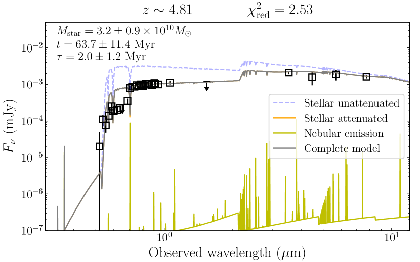
Figure 18: SSP model taken as the best solution for the no-Ly$\alpha$ LBG SHARDS J123757.50+621718.7. The absence of Ly$\alpha$ emission line makes it possible to fit the continuum of the SED even up to the IRAC measurements using a single relatively old, massive stellar population. Note that the nebular emission is so low that the complete spectrum practically corresponds to the attenuated stellar emission.

Knowing that the Ly$\alpha$ emission quickly decays within the first few Myr, we would expect to see a small fraction of objects presenting strong Ly$\alpha$ line emission among the LAE-LBGs population, which actually matches the EW distribution of this sample presented in Arrabal Haro et al. (2018). This is also the reason why we find only 404, out of 1,434, continuum sources with emission line. Indeed, we have detected 1,030 sources with no emission line, which would correspond to evolved galaxies with no significant young starburst at present. This represents the most common state of this type of high-$z$ galaxies, with the strong Ly$\alpha$ line emission being a recurrent and transiting episode in their lives. Nonetheless, it is also possible that in some sources, especially beyond $z\sim 5$, the Ly$\alpha$ photons are destroyed by scattering through a dense neutral medium as discussed in Hayes et al. (2010). Furthermore, a closer look to the Ly$\alpha$ EW of the LAEs (see Fig. 19) reveals no relation between that and the need of any extra SP for the LAE-LBGs, suggesting that the requirement of DSP models for these high-$z$ galaxies is given not only by their Ly$\alpha$ emission but by the relation between this and their emission at longer wavelengths, as also shown in Fig. 17, being the Ly$\alpha$ EW an indicator of the age in the SSP models, or of the relative strength of the young SP respect to the old one in the DSP models. On the other side, pure LAEs do show larger Ly$\alpha$ EWs, as expected from their observational definition. Additionally, the relative number of young LAEs increases with $z$ (see Fig. 20), while that of the old LBGs decreases, which also supports the scenario of an evolution from the pure LAE stage to the LBG, with a much larger proportion of sources in the younger stage the higher the redshift, decreasing as more evolved galaxies form and accumulate as we move to lower redshifts. This behaviour is also consistent with the study of the SFR density (SFRD) carried out by Sobral et al. (2018), who found an increasing trend with $z$ of the $\mathrm{SFRD_{Ly\alpha}/SFRD_{UV}}$ ratio at $z=2$-6.

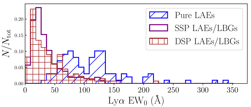
Figure 19: Rest-frame Ly$\alpha$ EW distribution of pure LAEs (blue diagonals), SSP LAE-LBGs (unfilled purple) and DSP LAE-LBGs (brown squares) weighted by the total amount of objects belonging to each subclass. No relation is found between Ly$\alpha$ EW and the need of a second SP when modelling the SEDs of LAE-LBGs.

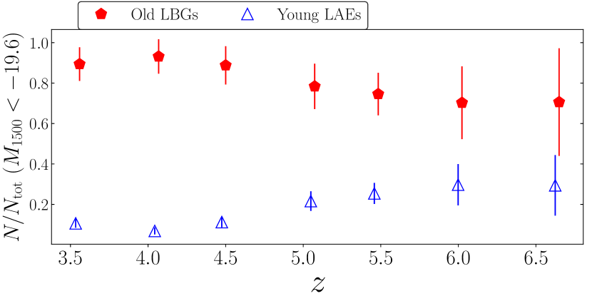
Figure 20: Amount of sources of each class respect to the total number of sources at each $z$ bin. Only objects brighter than $M_{1500}=-19.6$ have been considered, corresponding with the approximated 90% completeness at the highest $z$ bin. The sum of no-Ly$\alpha$ LBGs and DSP LAE-LBGs is represented by the red pentagons. Pure LAEs and SSP LAE-LBGs are represented by the blue empty triangles. The trend of these two groups is consistent with an evolutionary scenario between them.

5.2 SMFs and SMDs evolution

The obtained SMFs shown in Fig. 12 are in good agreement with previous estimations from similar studies where the stellar masses were derived through SED fitting. Note that the calculated SMFs are mostly driven by the LBGs population as the bulk of pure LAEs are found in a $M_{\mathrm{star}}$ range out of our completeness, as can be appreciated in Figs. 10 and 15. A non-negligible discrepancy can be noticed respect to other works where the UV luminosity was used to derive the $M_{\mathrm{star}}$ through the estimation of a tight mass-to-light ratio (Stark et al., 2009; González et al., 2011; Stefanon et al., 2017). This discrepancy between SED-fitted and $M_{\mathrm{UV}}$-derived $M_{\mathrm{star}}$ could appear due to small differences in the calculated $M/L$ relation, as discussed in Grazian et al. (2015). The SMF best-fitting Schechter parameters presented in Sec. 4.5 show a decreasing of the SMF with $z$. We find that the characteristic stellar mass $M^{*}$ shifts towards higher masses with cosmic time, as also found by Grazian et al. (2015). In particular, we measure $\log(M_{\mathrm{star}}/M_{\odot})=11.06^{+0.33}_{-0.27}$, $10.78^{+0.53}_{-0.07}$ and $10.51^{+0.08}_{-0.03}$ at $z\sim 4$, 5 and 6, respectively. No significant change is found for the low mass slope, from $\alpha=-1.72^{+0.24}_{-0.14}$ at $z\sim 4$ to $\alpha=-1.76^{+0.19}_{-0.26}$ at $z\sim 5$ with a slight increase to $-1.49^{+0.22}_{-0.21}$ at $z\sim 6$. However, the large uncertainty of this last measurement makes it difficult to measure a robust evolution of the $\alpha$ slope within our redshift range. In any case, our $\alpha$ values are much steeper than those found at low redshift, in agreement with previous estimations (e.g, Santini et al., 2012; Duncan et al., 2014; Grazian et al., 2015; Song et al., 2016; Davidzon et al., 2017; Stefanon et al., 2017).

The characterisation of the SMF has allowed us to estimate the SMD at each redshift through the integration of the SMF. The results shown in Fig. 13 are in good agreement with the general evolution of this magnitude with cosmic time presented in previous works. Apart from the large errors of the SMD estimation at $z\sim 5$-6 product of the already discussed uncertainty of the SMF low mass slope calculation at these redshifts, it is worth noticing that the decrease of SMD between $z\sim 4$-5 is softer than that between $z\sim 5$-6, suggesting that the SMD at $z\sim 5$ obtained in our field could be larger than expected following the general SMD-$z$ trend at $z=4$-6. This could be linked to the presence of a reported $z\sim 5.2$ overdensity in the GOODS-N field (Walter et al., 2012; Arrabal Haro et al., 2018).

5.3 SFR-$M_{\mathrm{star}}$ relation and stellar mass growth implications

Several authors have previously studied the SFR-$M_{\mathrm{star}}$ relation (Stark et al., 2009; González et al., 2010; Papovich et al., 2011; Salmon et al., 2015) also finding the same lack of evolution on its slope between $4\lesssim z\lesssim 6$ (see Figs. 14 and 15). The low scatter of this relation have suggested that galaxies at this epoch form stars in a larger rate the more massive they are. This supported the hypothesis of a constant pristine gas income over the evolution of these high-$z$ galaxies, leaving violent starburst episodes due to mergers or instabilities in a secondary role in the stellar mass growth of these galaxies. However, this stochastic events still likely alter the smooth increase of the $M_{\mathrm{star}}$, as also suggested in González et al. (2010) and Papovich et al. (2011). Our study shows that the assumption of bursty SFHs driving the growth of galaxies at $4\lesssim z\lesssim 6$ through episodic SF processes is also consistent with the presence of a tight SFR-$M_{\mathrm{star}}$ main sequence. It should be noticed that the SFRs derived in Arrabal Haro et al. (2018) from the $L_{1500}$ are the SFR averaged over the last 30-100 Myr it takes to the UV luminosity to change after SFR variations (e.g., Salim et al., 2009; Otí-Floranes & Mas-Hesse, 2010; Salmon et al., 2015). In this way, galaxies which are brighter in the UV do show higher SFRs according to the smooth growth scenario suggested by the SFR-$M_{\mathrm{star}}$ main sequence. Nevertheless, these UV brighter and more massive sources are not necessarily presenting the strongest Ly$\alpha$ emission lines, indicating a current ($\lesssim 25$ Myr) SF. Additionally, we find a majority of sources (1,030) with undetected Ly$\alpha$ line in our SEDs. These galaxies could still have a smooth and relatively slow star formation component, presenting faint Ly$\alpha$ emission which is not detected in the photometry, with those showing high Ly$\alpha$ EWs suffering a stochastic episode of SF on top of that. In fact, studying the SFR-$M_{\mathrm{star}}$ main sequence derived from the best-fitting SSP models (Fig. 15) we find that both pure LAEs and LAE-LBGs are placed above the mean main sequence, as also found in Santos et al. (2020), indicating that they are indeed experimenting a recent star-forming episode.

6 Conclusions.

We have used cigale to model the sample of high-$z$ LAEs and LBGs selected from the SHARDS survey in Arrabal Haro et al. (2018), consisting of 1,558 sources at $3.4<z<6.8$ in the GOODS-N field. Special attention is given to the differences between the three different subfamilies observationally defined in terms of their Ly$\alpha$ line and UV continuum emission. Single and double stellar population models are used to fit every SED, making use of a Bayesian information criterion calibration to decide in which situations an extra stellar population is needed. With the stellar masses derived from the models, we have studied the SMF, SMD and SFR-$M_{\mathrm{star}}$ relation at each $z$, as well as the evolution of the fraction of sources from each subclass. The main conclusions are the following:

1. The majority ($\sim 79\%$) of our high-$z$ LAEs and LBGs are well explained by a single stellar population. The cases better described with a secondary stellar population are still strongly dominated by the older population in terms of $M_{\mathrm{star}}$. However, the young stellar population is essential in terms of luminosity to properly fit the Ly$\alpha$ and rest-frame UV emission of these SEDs.

2. The relative amount of objects from each of the subfamilies that need an additional stellar population is not the same. We find that the LAE-LBGs require double stellar population models in $\sim$33% of the cases, in comparison with the $\sim$16% and $\sim$22% found for the no-Ly$\alpha$ LBGs and pure LAEs, respectively. The need of two populations in a significant fraction of the LAEs is due to the presence of a strong Ly$\alpha$ emission line combined with a bright continuum at the longest sampled wavelengths (IRAC) that cannot be simultaneously fitted well by a single stellar population, as in, e.g., Rodriguez Espinosa et al. (2014).

3. Pure LAEs can be tipically understood as very young and low mass galaxies with a median age of $\sim 26$ Myr and a median $M_{\mathrm{star}}$ of $\sim 5\times 10^{8}\ M_{\odot}$, presenting high Ly$\alpha$ EWs and experimenting one of their first star-forming episodes. The increasing fraction of these objects with $z$ in our sample, consistent with Sobral et al. (2018b), supports the hypothesis of these pure LAEs typically being an initial and transitional stage on the evolution of high-$z$ sources.

4. LAE-LBGs can be split into two subgroups differentiated in age and stellar mass properties. Single stellar population LAE-LBGs seem to be very young (median age of $\sim 27$ Myr) but slightly more massive on average than the pure LAEs (median $M_{\mathrm{star}}\sim 10^{9}\ M_{\odot}$). The similarities with the pure LAEs subclass suggests that these are members of the same kind of young galaxies, but with different SFRs and stellar masses. The relative number of young LAEs follows the same trend with $z$ than the pure LAEs one, supporting the idea of them being the same kind of galaxies.

5. Dual stellar population LAEs are fitted by older (hundreds of Myr) and more massive models ($M_{\mathrm{star}}\sim 10^{10}\ M_{\odot}$) featuring a young and much less massive population causing the bulk of the Ly$\alpha$ emission. According to this, double stellar population LAEs seem to be galaxies more massive and evolved (at this $z$), undergoing an episodic star-forming episode.

6. No-Ly$\alpha$ LBGs are the most difficult subclass to model, as they do not show emission patterns that strongly help to constrain their ages in the rest-frame wavelength range sampled in this work at these redshifts. This creates a degeneracy in the combinations of stellar populations that could lead to a good fit of their SEDs with negligible variations in the $\chi^{2}$. Moreover, some of these galaxies could actually host a very young stellar population whose Ly$\alpha$ line is not detected because of resonant scattering and dust extinction. Furthermore, the use of the Bayesian information criterion could be biasing the calculated ages for this family towards younger values, so we only aim to model these sources in a general way, being aware that the description of the class may not match all the individual cases.

7. With the caveats just mentioned, the results derived from cigale show that no-Ly$\alpha$ LBGs lack a really young SP ($\lesssim 25$ Myr). Furthermore, the absence of strong Ly$\alpha$ emission indicates that these sources are not in a current strong star-forming episode (or have extremely low escape fractions). However, it is possible that these galaxies present a fairly smooth star formation, producing faint Ly$\alpha$ lines which are not detected in the photometry. They are older and much more massive than pure LAEs or single stellar population LAE-LBGs, with a median $M_{\mathrm{star}}$ of $\sim 3.5\times 10^{9}\ M_{\odot}$. These results suggest that no-Ly$\alpha$ LBGs are a more evolved stage of high-$z$ galaxies that have been forming stars for a longer time, developing larger stellar masses and presenting brighter continuum emission at longest wavelengths, because of the old stars. The evolution of the fraction of these objects with $z$ also supports the idea of no-Ly$\alpha$ LBGs being more evolved star-forming sources, the more common the lower the $z$ is.

8. We report a decreasing evolution of the characteristic stellar mass of the SMFs with $z$, as in e.g., Grazian et al. (2015), finding $\log(M^{*}/M_{\odot})=11.06^{+0.33}_{-0.27}$, $10.78^{+0.53}_{-0.07}$ and $10.51^{+0.08}_{-0.03}$ at $z\sim 4$, 5 and 6, respectively. The low mass slopes found are steeper than those typically found at low redshift. No significant evolution is found between $z=4-$5, with a small increase at $z\sim 6$ ($\alpha=-1.72^{+0.24}_{-0.14}$, $-1.76^{+0.19}_{-0.26}$ and $-1.49^{+0.22}_{-0.21}$ at $z\sim 4$, 5 and 6, respectively). However, the $\alpha$ estimated at $z\sim 5$-6 has to be carefully considered, as we do not have much information covering the $M_{\mathrm{star}}$ region corresponding to the potential term of the Schechter SMF at these redshifts.

9. The SMD is estimated by integration of the SMF at each redshift. Our results are in agreement with the SMD-$z$ trend reported at these redshifts by previous authors (Labbé et al., 2010; González et al., 2011; Lee et al., 2012; Duncan et al., 2014; Grazian et al., 2015; Song et al., 2016). The SMD obtained at $z\sim 5$, although consistent with the general trend, is slightly larger than expected if we follow the mean slope of the SMD-$z$ relation at high-$z$, which could be linked to the presence of a previously reported $z\sim 5.2$ overdensity in GOODS-N (Walter et al., 2012; Arrabal Haro et al., 2018). Additional research is incoming to further characterise this overdensity.

10. The slope values found for the $\mathrm{SFR}\propto M_{\mathrm{star}}^{\beta}$ relation are $\beta=0.48^{+0.07}_{-0.10}$, $0.46^{+0.12}_{-0.10}$, $0.51^{+0.26}_{-0.19}$ at $z\sim 4$, 5 and 6, respectively, for the UV-derived SFRs and $\beta=0.83^{+0.09}_{-0.06}$, $0.79^{+0.10}_{-0.11}$, $0.82^{+0.15}_{-0.16}$ at $z\sim 4$, 5 and 6, respectively, for the model-derived SFRs, both of them consistent with little to no redshift evolution of that slope within that redshift range, in agreement with previous works (e.g., Stark et al., 2009; González et al., 2010; Papovich et al., 2011; Salmon et al., 2015). The existence of such tight relation between these two magnitudes and its invariability within this $z$ range point to the hypothesis of a smooth pristine gas infall as the main mechanism responsible of the mass growth of these galaxies along their lives, as suggested before. Nevertheless, the best-fitting burst-like SFHs used in this work also produce an equally tight main sequence. This, joined to the fact that LAEs appear above the SFR-$M_{\mathrm{star}}$ main sequence, supports the existence of stochastic star-forming events due to mergers and other instabilities that can also be responsible of the stellar mass growth in high-$z$ galaxies.

Appendix A Monte Carlo Schechter function fit to the SMF

In this appendix we show the confidence intervals of the Schechter parameters obtained using Monte Carlo simulations to fit the SMF. The perturbations in the measurements are implemented injecting a Gaussian noise to each point consistent with its own Poissonian error. Additionally, the $M_{\mathrm{star}}$ bins are also perturbed, both in size and centre value. In particular, the bin size is perturbed between 0.2-0.3 dex in intervals of 0.025 dex. The central $M_{\mathrm{star}}$ value of each bin is as well shifted 0.1 dex in intervals of 0.025 dex. At $z\sim 6$, using the SMF points up to the estimated stellar mass 90% completeness limit results in the inclusion of actually incomplete points close to the characteristic $M^{*}$ knee for several $M_{\mathrm{star}}$ bin perturbations, obtaining positive values for the low mass slope. To solve this issue, only strictly increasing SMF points are considered for the Schechter function fit as we move to lower stellar masses up to our $M_{\mathrm{star},\mathrm{lim}}$, as further points are considered incomplete. The $\alpha$ slope is also constrained to $-3.0<\alpha<-0.9$ for the fit. We are aware that this approach could bias our $z\sim 6$ low mass slope estimation towards steeper values, as warned in the text. The significance contours of the three Schechter parameters at $z\sim 4$, 5 and 6 are shown in Figs. 21, 22 and 23, respectively.

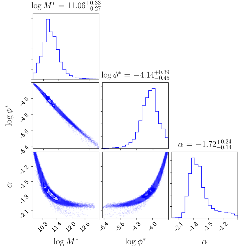
Figure 21: Confidence intervals on the Schechter parameters from the Monte Carlo fitting at $z\sim 4$. The inner and outer contours correspond to the $1\sigma$ and $3\sigma$ significance, respectively.

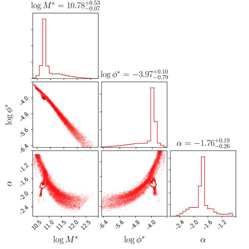
Figure 22: Confidence intervals on the Schechter parameters from the Monte Carlo fitting at $z\sim 5$. The inner and outer contours correspond to the $1\sigma$ and $3\sigma$ significance, respectively.

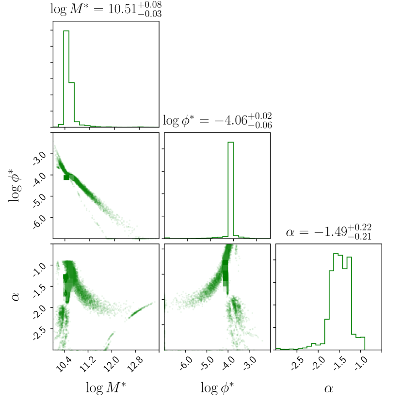
Figure 23: Confidence intervals on the Schechter parameters from the Monte Carlo fitting at $z\sim 6$. The inner and outer contours correspond to the $1\sigma$ and $3\sigma$ significance, respectively.

References

- Arrabal Haro et al. (2018) Arrabal Haro, P., Rodríguez Espinosa, J. M., Muñoz-Tuñón, C., et al. 2018, MNRAS, 478, 3740
- Ashby et al. (2015) Ashby, M. L. N., Willner, S. P., Fazio, G. G., et al. 2015, ApJS, 218, 33
- Barro et al. (2011) Barro, G., Pérez-González, P. G., Gallego, J., et al. 2011, ApJS, 193, 13
- Barro et al. (2011b) —. 2011b, ApJS, 193, 30
- Barro et al. (2019) Barro, G., Pérez-González, P. G., Cava, A., et al. 2019, ApJS, 243, 22
- Behroozi et al. (2013) Behroozi, P. S., Wechsler, R. H., & Conroy, C. 2013, ApJ, 770, 57
- Bina et al. (2016) Bina, D., Pelló, R., Richard, J., et al. 2016, A&A, 590, A14
- Boquien et al. (2014) Boquien, M., Buat, V., & Perret, V. 2014, A&A, 571, A72
- Boquien et al. (2016) Boquien, M., Kennicutt, R., Calzetti, D., et al. 2016, A&A, 591, A6
- Boquien et al. (2019) Boquien, M., Burgarella, D., Roehlly, Y., et al. 2019, A&A, 622, A103
- Bouwens et al. (2011) Bouwens, R. J., Illingworth, G. D., Labbe, I., et al. 2011, Nature, 469, 504
- Bouwens et al. (2014) Bouwens, R. J., Bradley, L., Zitrin, A., et al. 2014, ApJ, 795, 126
- Bouwens et al. (2015) Bouwens, R. J., Illingworth, G. D., Oesch, P. A., et al. 2015, ApJ, 803, 34
- Bruzual & Charlot (2003) Bruzual, G., & Charlot, S. 2003, MNRAS, 344, 1000
- Calzetti et al. (2000) Calzetti, D., Armus, L., Bohlin, R. C., et al. 2000, ApJ, 533, 682
- Caputi et al. (2011) Caputi, K. I., Cirasuolo, M., Dunlop, J. S., et al. 2011, MNRAS, 413, 162
- Caputi et al. (2015) Caputi, K. I., Ilbert, O., Laigle, C., et al. 2015, ApJ, 810, 73
- Carnall et al. (2019) Carnall, A. C., Leja, J., Johnson, B. D., et al. 2019, ApJ, 873, 44
- Cassata et al. (2015) Cassata, P., Tasca, L. A. M., Le Fèvre, O., et al. 2015, A&A, 573, A24
- Cava et al. (2015) Cava, A., Pérez-González, P. G., Eliche-Moral, M. C., et al. 2015, ApJ, 812, 155
- Davé et al. (2013) Davé, R., Katz, N., Oppenheimer, B. D., Kollmeier, J. A., & Weinberg, D. H. 2013, MNRAS, 434, 2645
- Davidzon et al. (2017) Davidzon, I., Ilbert, O., Laigle, C., et al. 2017, A&A, 605, A70
- Dayal & Ferrara (2012) Dayal, P., & Ferrara, A. 2012, MNRAS, 421, 2568
- Dickinson et al. (2003) Dickinson, M., Papovich, C., Ferguson, H. C., & Budavári, T. 2003, ApJ, 587, 25
- Drake et al. (2017) Drake, A. B., Guiderdoni, B., Blaizot, J., et al. 2017, MNRAS, 471, 267
- Drake et al. (2017b) Drake, A. B., Garel, T., Wisotzki, L., et al. 2017b, A&A, 608, A6
- Duncan et al. (2014) Duncan, K., Conselice, C. J., Mortlock, A., et al. 2014, MNRAS, 444, 2960
- Ellis et al. (2013) Ellis, R. S., McLure, R. J., Dunlop, J. S., et al. 2013, ApJ, 763, L7
- Fazio et al. (2004) Fazio, G. G., Ashby, M. L. N., Barmby, P., et al. 2004, ApJS, 154, 39
- Fontana et al. (2006) Fontana, A., Salimbeni, S., Grazian, A., et al. 2006, A&A, 459, 745
- Gawiser et al. (2006) Gawiser, E., van Dokkum, P. G., Gronwall, C., et al. 2006, ApJ, 642, L13
- Giavalisco et al. (1996) Giavalisco, M., Steidel, C. C., & Macchetto, F. D. 1996, ApJ, 470, 189
- Giavalisco (2002) Giavalisco, M. 2002, ARA&A, 40, 579
- Giavalisco et al. (2004) Giavalisco, M., Dickinson, M., Ferguson, H. C., et al. 2004, ApJ, 600, L103
- Giavalisco et al. (2004b) Giavalisco, M., Ferguson, H. C., Koekemoer, A. M., et al. 2004b, ApJ, 600, L93
- González et al. (2010) González, V., Labbé, I., Bouwens, R. J., et al. 2010, ApJ, 713, 115
- González et al. (2011) —. 2011, ApJ, 735, L34
- Grazian et al. (2015) Grazian, A., Fontana, A., Santini, P., et al. 2015, A&A, 575, A96
- Grogin et al. (2011) Grogin, N. A., Kocevski, D. D., Faber, S. M., et al. 2011, ApJS, 197, 35
- Gronwall et al. (2007) Gronwall, C., Ciardullo, R., Hickey, T., et al. 2007, ApJ, 667, 79
- Hayes et al. (2010) Hayes, M., Östlin, G., Schaerer, D., et al. 2010, Nature, 464, 562
- Hayes et al. (2011) Hayes, M., Schaerer, D., Östlin, G., et al. 2011, ApJ, 730, 8
- Hernán-Caballero et al. (2017) Hernán-Caballero, A., Pérez-González, P. G., Diego, J. M., et al. 2017, ApJ, 849, 82
- Hu et al. (1998) Hu, E. M., Cowie, L. L., & McMahon, R. G. 1998, ApJ, 502, L99
- Ilbert et al. (2013) Ilbert, O., McCracken, H. J., Le Fèvre, O., et al. 2013, A&A, 556, A55
- Inoue (2011) Inoue, A. K. 2011, MNRAS, 415, 2920
- Iwata et al. (2007) Iwata, I., Ohta, K., Tamura, N., et al. 2007, MNRAS, 376, 1557
- Iye et al. (2006) Iye, M., Ota, K., Kashikawa, N., et al. 2006, Nature, 443, 186
- Iye (2011) Iye, M. 2011, Proceedings of the Japan Academy. Series B, Physical and biological sciences, 87, 575—586
- Jiang et al. (2016) Jiang, L., Finlator, K., Cohen, S. H., et al. 2016, ApJ, 816, 16
- Kajisawa et al. (2009) Kajisawa, M., Ichikawa, T., Tanaka, I., et al. 2009, ApJ, 702, 1393
- Kennicutt (1998) Kennicutt, Robert C., J. 1998, ApJ, 498, 541
- Koekemoer et al. (2011) Koekemoer, A. M., Faber, S. M., Ferguson, H. C., et al. 2011, ApJS, 197, 36
- Koo & Kron (1980) Koo, D. C., & Kron, R. T. 1980, PASP, 92, 537
- Labbé et al. (2010) Labbé, I., González, V., Bouwens, R. J., et al. 2010, ApJ, 716, L103
- Laidler et al. (2007) Laidler, V. G., Papovich, C., Grogin, N. A., et al. 2007, PASP, 119, 1325
- Laporte et al. (2016) Laporte, N., Infante, L., Troncoso Iribarren, P., et al. 2016, ApJ, 820, 98
- Lee et al. (2012) Lee, K.-S., Ferguson, H. C., Wiklind, T., et al. 2012, ApJ, 752, 66
- Leja et al. (2019) Leja, J., Carnall, A. C., Johnson, B. D., Conroy, C., & Speagle, J. S. 2019, ApJ, 876, 3
- Liddle (2007) Liddle, A. R. 2007, MNRAS, 377, L74
- Lumbreras-Calle et al. (2019) Lumbreras-Calle, A., Muñoz-Tuñón, C., Méndez-Abreu, J., et al. 2019, A&A, 621, A52
- Madau et al. (1998) Madau, P., Pozzetti, L., & Dickinson, M. 1998, ApJ, 498, 106
- Malhotra & Rhoads (2004) Malhotra, S., & Rhoads, J. E. 2004, ApJ, 617, L5
- Marchesini et al. (2009) Marchesini, D., van Dokkum, P. G., Förster Schreiber, N. M., et al. 2009, ApJ, 701, 1765
- Marchesini et al. (2010) Marchesini, D., Whitaker, K. E., Brammer, G., et al. 2010, ApJ, 725, 1277
- Matthee et al. (2016) Matthee, J., Sobral, D., Oteo, I., et al. 2016, MNRAS, 458, 449
- Matthee et al. (2017) Matthee, J., Sobral, D., Darvish, B., et al. 2017, MNRAS, 472, 772
- McLure et al. (2009) McLure, R. J., Cirasuolo, M., Dunlop, J. S., Foucaud, S., & Almaini, O. 2009, MNRAS, 395, 2196
- Méndez-Abreu et al. (2018) Méndez-Abreu, J., Aguerri, J. A. L., Falcón-Barroso, J., et al. 2018, MNRAS, 474, 1307
- Mortlock et al. (2011) Mortlock, A., Conselice, C. J., Bluck, A. F. L., et al. 2011, MNRAS, 413, 2845
- Muzzin et al. (2013) Muzzin, A., Marchesini, D., Stefanon, M., et al. 2013, ApJ, 777, 18
- Noll et al. (2009) Noll, S., Burgarella, D., Giovannoli, E., et al. 2009, A&A, 507, 1793
- Oesch et al. (2010) Oesch, P. A., Bouwens, R. J., Illingworth, G. D., et al. 2010, ApJ, 709, L16
- Oke & Gunn (1983) Oke, J. B., & Gunn, J. E. 1983, ApJ, 266, 713
- Otí-Floranes & Mas-Hesse (2010) Otí-Floranes, H., & Mas-Hesse, J. M. 2010, A&A, 511, A61
- Ouchi et al. (2008) Ouchi, M., Shimasaku, K., Akiyama, M., et al. 2008, ApJS, 176, 301
- Ouchi et al. (2009) Ouchi, M., Ono, Y., Egami, E., et al. 2009, ApJ, 696, 1164
- Ouchi et al. (2010) Ouchi, M., Shimasaku, K., Furusawa, H., et al. 2010, ApJ, 723, 869
- Papovich et al. (2001) Papovich, C., Dickinson, M., & Ferguson, H. C. 2001, ApJ, 559, 620
- Papovich et al. (2011) Papovich, C., Finkelstein, S. L., Ferguson, H. C., Lotz, J. M., & Giavalisco, M. 2011, MNRAS, 412, 1123
- Pérez-González et al. (2003) Pérez-González, P. G., Gil de Paz, A., Zamorano, J., et al. 2003, MNRAS, 338, 508
- Pérez-González et al. (2005) Pérez-González, P. G., Rieke, G. H., Egami, E., et al. 2005, ApJ, 630, 82
- Pérez-González et al. (2008) Pérez-González, P. G., Rieke, G. H., Villar, V., et al. 2008, ApJ, 675, 234
- Pérez-González et al. (2013) Pérez-González, P. G., Cava, A., Barro, G., et al. 2013, ApJ, 762, 46
- Planck Collaboration et al. (2016) Planck Collaboration, Ade, P. A. R., Aghanim, N., et al. 2016, A&A, 594, A13
- Pozzetti et al. (2007) Pozzetti, L., Bolzonella, M., Lamareille, F., et al. 2007, A&A, 474, 443
- Pozzetti et al. (2010) Pozzetti, L., Bolzonella, M., Zucca, E., et al. 2010, A&A, 523, A13
- Riess et al. (2007) Riess, A. G., Strolger, L.-G., Casertano, S., et al. 2007, ApJ, 659, 98
- Robertson et al. (2010) Robertson, B. E., Ellis, R. S., Dunlop, J. S., McLure, R. J., & Stark, D. P. 2010, Nature, 468, 49
- Rodriguez Espinosa et al. (2014) Rodriguez Espinosa, J. M., Gonzalez-Martin, O., Castro-Rodriguez, N., et al. 2014, MNRAS, 444, L68
- Salim et al. (2009) Salim, S., Dickinson, M., Michael Rich, R., et al. 2009, ApJ, 700, 161
- Salmon et al. (2015) Salmon, B., Papovich, C., Finkelstein, S. L., et al. 2015, ApJ, 799, 183
- Salpeter (1955) Salpeter, E. E. 1955, ApJ, 121, 161
- Santini et al. (2012) Santini, P., Fontana, A., Grazian, A., et al. 2012, A&A, 538, A33
- Santos et al. (2016) Santos, S., Sobral, D., & Matthee, J. 2016, MNRAS, 463, 1678
- Santos et al. (2020) Santos, S., Sobral, D., Matthee, J., et al. 2020, MNRAS, 493, 141
- Schechter (1976) Schechter, P. 1976, ApJ, 203, 297
- Schlafly & Finkbeiner (2011) Schlafly, E. F., & Finkbeiner, D. P. 2011, ApJ, 737, 103
- Schmidt (1968) Schmidt, M. 1968, ApJ, 151, 393
- Schwarz (1978) Schwarz, G. E. 1978, Ann. Stat., 6, 461
- Serra et al. (2011) Serra, P., Amblard, A., Temi, P., et al. 2011, ApJ, 740, 22
- Sobral et al. (2017) Sobral, D., Matthee, J., Best, P., et al. 2017, MNRAS, 466, 1242
- Sobral et al. (2018) Sobral, D., Santos, S., Matthee, J., et al. 2018, MNRAS, 476, 4725
- Sobral et al. (2018b) Sobral, D., Matthee, J., Darvish, B., et al. 2018b, MNRAS, 477, 2817
- Sobral & Matthee (2019) Sobral, D., & Matthee, J. 2019, A&A, 623, A157
- Song et al. (2016) Song, M., Finkelstein, S. L., Ashby, M. L. N., et al. 2016, ApJ, 825, 5
- Stark et al. (2009) Stark, D. P., Ellis, R. S., Bunker, A., et al. 2009, ApJ, 697, 1493
- Stefanon et al. (2017) Stefanon, M., Bouwens, R. J., Labbé, I., et al. 2017, ApJ, 843, 36
- Steidel & Hamilton (1993) Steidel, C. C., & Hamilton, D. 1993, AJ, 105, 2017
- Steidel et al. (2003) Steidel, C. C., Adelberger, K. L., Shapley, A. E., et al. 2003, ApJ, 592, 728
- Taniguchi et al. (2005) Taniguchi, Y., Ajiki, M., Nagao, T., et al. 2005, PASJ, 57, 165
- Tomczak et al. (2014) Tomczak, A. R., Quadri, R. F., Tran, K.-V. H., et al. 2014, ApJ, 783, 85
- Trainor et al. (2015) Trainor, R. F., Steidel, C. C., Strom, A. L., & Rudie, G. C. 2015, ApJ, 809, 89
- Trainor et al. (2016) Trainor, R. F., Strom, A. L., Steidel, C. C., & Rudie, G. C. 2016, ApJ, 832, 171
- Walter et al. (2012) Walter, F., Decarli, R., Carilli, C., et al. 2012, Nature, 486, 233
- Yuma et al. (2010) Yuma, S., Ohta, K., Yabe, K., et al. 2010, ApJ, 720, 1016
- van der Burg et al. (2010) van der Burg, R. F. J., Hildebrandt, H., & Erben, T. 2010, A&A, 523, A74