Flexible framework for audio reconstruction

Abstract

The paper presents a unified, flexible framework for the tasks of audio inpainting, declipping, and dequantization. The concept is further extended to cover analogous degradation models in a transformed domain, e.g. quantization of the signal’s time-frequency coefficients. The task of reconstructing an audio signal from degraded observations in two different domains is formulated as an inverse problem, and several algorithmic solutions are developed. The viability of the presented concept is demonstrated on an example where audio reconstruction from partial and quantized observations of both the time-domain signal and its time-frequency coefficients is carried out.

1 Introduction

Audio inpainting, audio declipping and audio dequantization are reconstruction tasks that are usually studied separately in the literature. In audio inpainting, some of the time-domain signal samples are completely missing and they need to be recovered, while in the cases of declipping and dequantization, the samples are not lost fully and the samples to be recovered are known to lie in prescribed numerical ranges, depending on the model of the degradation. The feasibility set is called consistent if any solution, when exposed to the considered degradation model, produces exactly the observed signal. For example, in the case of audio inpainting, this shall be understood such that the reliable samples are kept intact.

A unification of different audio reconstruction tasks has partially been discussed in [1], where the authors covered dequantization and declipping (possibly at the same time), and in [2, 3], whose formulation allowed denoising and declipping (but not simultaneously). A flexible algorithmic framework is also presented in [4], based on the non-negative matrix factorization (which is shown to be suitable for simultaneous audio declipping and click concealment). The present article shows how the three tasks can be covered by a unified restoration framework, all of them possibly taking effect at the same time. The greatest contrast to the earlier attempts is, however, that this paper extends the range of degradation models by additionally considering a transformed domain. This is to say, the missing, clipped and quantized observations are further allowed after (linearly) transforming the signal, e.g. by the Short-time Fourier transform.

In Section 2, we introduce the three respective audio degradation models in more detail, emphasize their common factors, and build a set of feasible time-domain signals, which contains the potential solutions to the recovery task. We then extend the degradation to the transformed domain and present the synthesis and analysis variants of the resulting feasible set.

Finding a solution to any of the described recovery tasks is generally ill-posed. A regularizer is needed to pick favorable candidates from the feasibility set. The sparsity of time-frequency-transformed audio signals has been shown to be a suitable regularizer for audio recovery problems [5, 6, 7, 8]. Thus, Section 3 presents a general optimization problem with a special emphasis on using the $\ell_{1}$ relaxation of true sparsity. The section also presents a single, unified algorithm to find the numerical solution in the case of a convex regularizer.

In Section 4, we present a proof-of-concept example of an audio codec (i.e. coder and decoder). In the coder part, the original, input audio signal is due to subsampling and quantization in both the time and the time-frequency (TF) domains. The decoder attempts to recover the signal from this partial information, based on the assumption of sparsity of the (now unknown) original. Today’s audio codecs are built on the single-domain information, for instance the classical MPEG model codes the TF coefficients only, based on the global masking threshold estimate [9]. Recovery from quantized transformed observations is also studied in [10] in the context of compressed sensing. An interesting recent approach from [11], which is inspired in the image processing field, subsamples and quantizes purely time-domain audio samples to achieve compression. We show experimentally that in contrast to that approach, splitting the available bit budget between the two domains can be beneficial in some cases.

2 Building the framework

2.1 Time-frequency representations

In audio processing, TF operators are usually used to provide a suitable representation of a signal [12]. A signal $\mathbf{x}\in\mathbb{R}^{P}$ is represented as a superposition of time-localized oscillations, where the localization is due to the so-called window function that moves along the signal. Among such TF operators, the so-called tight frames are usually preferred, since they provide effective handling of both theoretical derivations and practical computations [12, 13, 14]. The Short-time Fourier (STFT, also known as the Gabor transform) or the Modified Discrete Cosine (MDCT) transforms [5, 15] are classical examples of such operators.

Throughout the paper, we use the following convention: To obtain an expansion of a signal $\mathbf{x}\in\mathbb{R}^{P}$ to a series of TF coefficients, the analysis operator $A\colon\mathbb{R}^{P}\to\mathbb{C}^{Q}$ is applied, where we assume $Q\geq P$. Its adjoint, the synthesis operator $A^{*}\colon\mathbb{C}^{Q}\to\mathbb{R}^{P}$​, reproduces the time-domain signal from the coefficients.

A tight frame with frame bound $\alpha$ can be characterized by the property $A^{*}\!A=\alpha\mathrm{Id}$, where $\mathrm{Id}$ is the identity operator, here on the space $\mathbb{R}^{P}$. When the constant $\alpha=1$, the frame is said to be Parseval tight.

2.2 Inpainting

Audio inpainting is a general term for recovering missing or highly degraded samples of the audio signal [5]. Suppose $\mathbf{y}\in\mathbb{R}^{P}$ is the original, non-degraded signal, and $M\mathbf{y}$ is the partial observation of $\mathbf{y}$. The operator $M\colon\mathbb{R}^{P}\to\mathbb{R}^{P}$ keeps the reliable samples, while putting zeros at the positions of missing or unreliable samples; these positions are assumed to be known. Thus, $M$ can be identified with a diagonal matrix $\mathbf{M}$ of size $P\times P$, for which $m_{pp}=1$ for a reliable sample $y_{p}$, $p=1,\ldots,P$, and zero otherwise. The solution of the inpainting problem is supposed to lie in a naturally defined set $\Gamma_{\mathrm{T}}^{\mathrm{inp}}=\left\{\mathbf{x}\in\mathbb{R}^{P}\mid M\mathbf{x}=M\mathbf{y}\right\},$ where the subscript indicates that it is defined in the time domain.

Clearly, defining the feasible set alone is not sufficient to solve the inpainting problem, since the inverse problem is ill-posed. Thus, the path to a solution must start from a careful consideration of additional assumptions about the signal. To name but a few, the solution may be modeled as an autoregressive process [16, 17], as a sum of sinusoidal components [18], or it is assumed to be sparse with respect to a suitable TF transform [5, 7, 19].

For the purpose of further generalization, the time-domain set $\Gamma_{\mathrm{T}}^{\mathrm{inp}}$ may be equivalently defined entrywise as

$$\mathbf{x}\in\Gamma_{\mathrm{T}}^{\mathrm{inp}}\;\Leftrightarrow\;\begin{cases}&x_{p}\in[y_{p},y_{p}]\ \text{for reliable indexes }p,\\ &x_{p}\in(-\infty,+\infty)\ \text{otherwise}.\end{cases}$$ (1)

2.3 Declipping

Audio declipping aims at recovering a signal damaged by clipping. This negative effect is one of the common audio degradation types and it can be described as a non-linear distortion causing a limitation of a signal, such that all values of the signal exceeding the allowed dynamic range defined by thresholds $[-\theta,\theta]$ are strictly limited by these thresholds. Because of the strict limitation of signal samples, the effect is also referred to as hard clipping. Not only does the information contained in the peaks get lost, but clipping also introduces a great number of higher harmonics, which leads to a significant reduction in the perceived audio quality [20] and also in the accuracy of automatic voice recognition [21].

Audio declipping is similar to audio inpainting, with the difference that in the case of audio declipping, the additional information (lower or upper bounds) about the clipped samples is available. Simple inpainting methods are able to effectively perform declipping, such as the Janssen method used in [5]. In general, however, inpainting approaches to declipping do not guarantee the consistency of the solution with the clipping constraints.

Similarly to the inpainting case, the set of feasible solutions, $\Gamma_{\mathrm{T}}^{\mathrm{dec}}$, is defined entrywise, taking advantage of the information that declipped samples need to exceed the clipping thresholds:

$$\mathbf{x}\in\Gamma_{\mathrm{T}}^{\mathrm{dec}}\Leftrightarrow\begin{cases}&x_{p}\in[y_{p},y_{p}]\ \text{for reliable samples}\ y_{p},\\ &x_{p}\in({-}\infty,{-}\theta]\ \text{for observed samples}\ {-}\theta,\\ &x_{p}\in[\theta,+\infty)\ \text{for observed samples}\ \theta.\end{cases}$$ (2)

2.4 Dequantization

The term dequantization refers to an inverse problem where a signal should be recovered based on the knowledge of its quantized observation. In this subsection, the quantization acts in the time domain, i.e. directly on the audio samples; the original sample is substituted with the value of the nearest quantization level. The unique quantization level is identified using a pair of the nearest so-called decision levels [22].

More specifically, assume a series of quantization levels

$$\dots<q_{-1}<q_{0}<q_{1}<q_{2}<\dots,$$ (3)

where this sequence can be theoretically infinite (but is always finite in practice). For a given $p$ and an input sample $y_{p}$ there exists a unique $n$ such that it holds $q_{n}\leq y_{p}<q_{n+1}$. Based on the decision level $d_{n}$, for which $q_{n}<d_{n}<q_{n+1}$, quantization maps $y_{p}$ either to $q_{n}$ (when $y_{p}<d_{n}$) or to $q_{n+1}$ (when $y_{p}\geq d_{n}$). In turn, if a quantized value $y_{p}^{\mathrm{quant}}$ is observed, there exists a single interval $[d_{n},d_{n+1})$ to which $y_{p}$ belongs.

Therefore, for the purpose of formulating a general problem, the set of feasible solutions is defined as the box-type set $\Gamma_{\mathrm{T}}^{\mathrm{deq}}$,

$$\mathbf{x}\in\Gamma_{\mathrm{T}}^{\mathrm{deq}}\;\Leftrightarrow\;x_{p}\in[d_{n},d_{n+1}),$$ (4)

where $d_{n}$ and $d_{n+1}$ (the closest lower and the closest upper decision levels to $y_{p}$, respectively) change depending on $p$, which is intentionally not reflected by the notation. Note also that in the finite case, border cases can be treated by using $\pm\infty$ in place of the lower or the upper bound in (4). In such a case, the half-open interval should be replaced by an open interval.

2.5 General formulation

When working with digital signals, clipping can be seen as a special kind of quantization. In such a case, the set of quantization levels defined by Eq. (3) corresponds exactly to the set of all possible numerical values in the range $[-\theta,\theta]$.

Looking at definitions (1), (2) and (4), one may observe that it is straightforward to define a feasible set for simultaneous audio inpainting, declipping and dequantization. Such a set is defined entrywise as a multidimensional interval $\Gamma_{\mathrm{T}}$ such that

$$\mathbf{x}\in\Gamma_{\mathrm{T}}\;\Leftrightarrow\;x_{p}\in[l_{\mathrm{T}p},u_{\mathrm{T}p}],\quad p=1,2,\ldots,P,$$ (5)

where the entries of the vector lower bound $\mathbf{l}_{\mathrm{T}}$ and the vector upper bound $\mathbf{u}_{\mathrm{T}}$ depend on the type of degradation that occurs at the index $p$, $p=1,\ldots,P$. One can think of $\Gamma_{\mathrm{T}}$ as a box in the $P$-dimensional space with its walls always parallel to an axis. The bounds may formally be plus or minus infinity, and in such a case, the box is infinitely wide in the respective directions.

It is straightforward to show that the set $\Gamma_{\mathrm{T}}$ is convex. Furthermore, solving an inverse problem with such a set of feasible solutions is tractable since the projection onto this type of set is available explicitly and entrywise by

$$\left(\mathrm{proj}_{\Gamma_{\mathrm{T}}}(\mathbf{x})\right)_{p}=\min\left\{u_{\mathrm{T}p},\max\left\{x_{p},l_{\mathrm{T}p}\right\}\right\}.$$ (6)

2.6 Feasible set in a transformed domain

So far, only time-domain degradation has been considered, leading to the set $\Gamma_{\mathrm{T}}$. Nevertheless, degradation as presented above can also happen in a transformed domain. The aim of this section is to generalize the above concept to both the time and the TF domains.

Similarly to (5), we define a feasible set within the TF domain. Such a domain is generally a subset of $\mathbb{C}^{Q}$. Any interval shall be understood in such a way that the real and imaginary parts are considered independently. As an example, for $l,u\in\mathbb{C}$, we denote

$$z\in[l,u]\;\Leftrightarrow\;\Re(z)\in[\Re(l),\Re(u)]\wedge\Im(z)\in[\Im(l),\Im(u)].$$ (7)

With such a notation, we define the membership in $\Gamma_{\mathrm{TF}}$ as

$$\mathbf{z}\in\Gamma_{\mathrm{TF}}\;\Leftrightarrow\;z_{q}\in[l_{\mathrm{TF}q},u_{\mathrm{TF}q}],\quad q=1,2,\ldots,Q.$$ (8)

The vector bounds $\mathbf{l}_{\mathrm{TF}},\mathbf{u}_{\mathrm{TF}}\in\mathbb{C}^{Q}$ determine for each coefficient whether its clipped or quantized version is observed or whether the coefficient is missing.

Combining the constraints in the two domains reduces the size of the overall feasible set. In general, however, this is not enough, and additional prior information is necessary.

2.7 Defining a prior

For the purpose of the general framework, assume some knowledge about the TF coefficients invoked by minimizing a functional $\mathcal{S}\circ W$. As a particular example, consider the (relaxed) sparse prior, namely $(\mathcal{S}\circ W)(\mathbf{z})=\mathcal{S}(W\mathbf{z})=\|W\mathbf{z}\|_{1}$, where $W$ is a diagonal operator assigning weights to the respective coefficients. The $\ell_{1}$ norm sums the magnitudes of the elements of its argument [23].

Combining the prior and the feasible sets $\Gamma_{\mathrm{T}}$ and $\Gamma_{\mathrm{TF}}$ provides us with the following general formulation:

$$\mathop{\operatorname{arg\leavevmode\nobreak\ min}}_{\mathbf{u}}\ \mathcal{S}(W\!K\mathbf{u})\quad\text{subject to}\quad L\mathbf{u}\in\Gamma_{\mathrm{T}},\;K\mathbf{u}\in\Gamma_{\mathrm{TF}}.$$ (9)

The linear operators $K$ and $L$ play the role of either the synthesis or the analysis operator of a suitable TF transform. In a typical situation, one of them will be identity. Such a notation may look redundant, but the reason for this shape of the formulation (9) is that it covers both the synthesis variant ($L=A^{*}$, $K=\mathrm{Id}$)

$$\mathop{\operatorname{arg\leavevmode\nobreak\ min}}_{\mathbf{z}}\ \mathcal{S}(W\mathbf{z})\quad\text{subject to}\quad A^{*}\mathbf{z}\in\Gamma_{\mathrm{T}},\;\mathbf{z}\in\Gamma_{\mathrm{TF}},$$ (10)

and the analysis variant ($L=\mathrm{Id}$, $K=A$):

$$\mathop{\operatorname{arg\leavevmode\nobreak\ min}}_{\mathbf{x}}\ \mathcal{S}(W\!A\mathbf{x})\quad\text{subject to}\quad\mathbf{x}\in\Gamma_{\mathrm{T}},\;A\mathbf{x}\in\Gamma_{\mathrm{TF}}.$$ (11)

Note that if a non-unitary transform $A$ is used, the formulations (10) and (11) are not equivalent. Also, the feasible sets in Eq. (10) and (11) may differ, as in the case of a non-tight frame.

3 Solving the task

The important observation about the sets $\Gamma_{\mathrm{T}}$ and $\Gamma_{\mathrm{TF}}$ defined by (5) and (8), respectively, is that both are box-type (and thus convex) sets. Furthermore, both the sets $\Gamma_{L}=\left\{\mathbf{u}\mid L\mathbf{u}\in\Gamma_{\mathrm{T}}\right\}$ and $\Gamma_{K}=\left\{\mathbf{u}\mid K\mathbf{u}\in\Gamma_{\mathrm{TF}}\right\}$ are convex as well. The reason is that the preimage of a convex set under a linear operator is a convex set, which is straightforward to show. Finally, the intersection of two convex sets is once again a convex set, therefore the set of feasible solutions in the constrained formulation (9) is convex for arbitrary linear operators $L$ and $K$.

However, such an intersection is a rather complicated set. One of the sets $\Gamma_{L}$ and $\Gamma_{K}$ is no longer a simple box-type set, hence the intersection $\Gamma_{L}\cap\Gamma_{K}$ is generally a polyhedron either in the time domain (for the analysis model) or in the TF domain (for the synthesis model). Still, it remains a non-empty set, since it must contain at least the original, non-degraded signal or coefficients. Thus, the formulation (9) has a solution.

Input: The linear operators $L_{m},\;m=1,\dots,M$, the proximal operators $\mathrm{prox}_{h_{m}},\;m=1,\dots,M$, $\mathrm{prox}_{g}$ and the gradient $\nabla f$.

1 Choose the parameters $\tau,\sigma,\rho>0$.

2 Choose the initial estimates $\mathbf{u}^{(0)},\mathbf{v}^{(0)}_{1},\dots,\mathbf{v}^{(0)}_{M}$.

3 for $i=0,1,\dots$ do

4       for $m=1,\dots,M$ do

5             $\tilde{\mathbf{v}}_{m}^{(i+1)}=\mathrm{prox}_{\sigma h_{m}^{*}}\left(\mathbf{v}_{m}^{(i)}+\sigma L_{m}\mathbf{u}^{(i)}\right)$

6             $\mathbf{v}_{m}^{(i+1)}=\rho\tilde{\mathbf{v}}_{m}^{(i+1)}+(1-\rho)\mathbf{v}_{m}^{(i)}$

7            

8       end for

9      $\tilde{\mathbf{u}}^{(i+1)}=\mathrm{prox}_{\tau g}\left(\mathbf{u}^{(i)}-\tau\nabla f\left(\mathbf{u}^{(i)}\right)-\tau\sum L_{m}^{*}\left(2\tilde{\mathbf{v}}_{m}^{(i+1)}-\mathbf{v}_{m}^{(i)}\right)\right)$

10       $\mathbf{u}^{(i+1)}=\rho\tilde{\mathbf{u}}^{(i+1)}+(1-\rho)\mathbf{u}^{(i)}$

11 end for

Output: $\mathbf{u}^{(i+1)}$

Algorithm 1 The CV algorithm for solving (13)

3.1 Consistent convex approach, arbitrary linear operators

We focus on the case when the function $\mathcal{S}$ is convex, thus the whole problem is convex. Convexity implies that the there exists a single global minimum. The idea is to use a proximal splitting method [24] to solve the formulation (9) numerically, which allows us to focus separately on operations related to the function $\mathcal{S}$, to the constraint $\mathbf{u}\in\Gamma_{L}$ and to the constraint $\mathbf{u}\in\Gamma_{K}$.

In the following, the notion of the proximal operator will be needed. The proximal operator of a proper convex lower semi-continuous function $h\colon\mathbb{V}\to\mathbb{R}$ is a mapping from $\mathbb{V}$ to $\mathbb{V}$ defined at any point $\mathbf{u}\in\mathbb{V}$ by the minimization problem $\mathrm{prox}_{h}(\mathbf{u})=\mathop{\operatorname{arg\leavevmode\nobreak\ min}}_{\mathbf{v}}\left\{h(\mathbf{v})+\frac{1}{2}\|\mathbf{v}-\mathbf{u}\|^{2}\right\}.$ Here, $\mathbb{V}$ stands for the Hilbert space $\mathbb{R}^{P}$ or $\mathbb{C}^{Q}$.

To design a particular proximal algorithm, the formulation (9) is first rewritten into the unconstrained form using the so-called indicator function $\iota_{\Gamma}$ of the set $\Gamma$. For $\mathbf{u}\in\Gamma$, the function returns 0, and $\infty$ otherwise. The formulation (9) thus attains the form

$$\mathop{\operatorname{arg\leavevmode\nobreak\ min}}_{\mathbf{u}}\left\{\mathcal{S}(W\!K\mathbf{u})+\iota_{\Gamma_{\mathrm{T}}}\left(L\mathbf{u}\right)+\iota_{\Gamma_{\mathrm{TF}}}\left(K\mathbf{u}\right)\right\}.$$ (12)

The unconstrained form is suitable for the use of the generic proximal algorithm proposed independently by Condat [25] and Vũ [26] (further referred to as the CV algorithm). It is tailored to solve problems of the form

$$\mathop{\operatorname{arg\leavevmode\nobreak\ min}}_{\mathbf{u}}\left\{f(\mathbf{u})+g(\mathbf{u})+\sum_{m=1}^{M}h_{m}(L_{m}\mathbf{u})\right\},$$ (13)

where $f,g,h_{1},\dots,h_{m}$ are convex lower semi-continuous functions, $f$ is differentiable, and $L_{1},\dots,L_{m}$ are bounded linear operators. We will utilize the second of the two proposed variants from [25], the general form of which is reproduced in Alg. 1.

Input: The linear operators $W,K,L$, the proximal operator $\mathrm{prox}_{\mathcal{S}}$ and the projectors $\mathrm{proj}_{\Gamma_{\mathrm{T}}},\mathrm{proj}_{\Gamma_{\mathrm{TF}}}$.

1 Choose the parameters $\tau,\sigma,\rho>0$ satisfying the conditions (14).

2 Choose the initial estimates $\mathbf{u}^{(0)},\mathbf{v}_{1}^{(0)},\mathbf{v}_{2}^{(0)},\mathbf{v}_{3}^{(0)}$.

3 for $i=0,1,\dots$ do

       /* update corresponding to $h_{1}$ */

4       $\tilde{\mathbf{v}}_{1}^{(i+1)}=\mathbf{v}_{1}^{(i)}+\sigma WK\mathbf{u}^{(i)}-\sigma\mathrm{prox}_{\mathcal{S}/\sigma}\left(\mathbf{v}_{1}^{(i)}/\sigma+WK\mathbf{u}^{(i)}\right)$

5       $\mathbf{v}_{1}^{(i+1)}=\rho\tilde{\mathbf{v}}_{1}^{(i+1)}+(1-\rho)\mathbf{v}_{1}^{(i)}$

       /* update corresponding to $h_{2}$ */

6       $\tilde{\mathbf{v}}_{2}^{(i+1)}=\mathbf{v}_{2}^{(i)}+\sigma L\mathbf{u}^{(i)}-\sigma\mathrm{proj}_{\Gamma_{\mathrm{T}}}\left(\mathbf{v}_{2}^{(i)}/\sigma+L\mathbf{u}^{(i)}\right)$

7       $\mathbf{v}_{2}^{(i+1)}=\rho\tilde{\mathbf{v}}_{2}^{(i+1)}+(1-\rho)\mathbf{v}_{2}^{(i)}$

       /* update corresponding to $h_{3}$ */

8       $\tilde{\mathbf{v}}_{3}^{(i+1)}=\mathbf{v}_{3}^{(i)}+\sigma K\mathbf{u}^{(i)}-\sigma\mathrm{proj}_{\Gamma_{\mathrm{TF}}}\left(\mathbf{v}_{3}^{(i)}/\sigma+K\mathbf{u}^{(i)}\right)$

9       $\mathbf{v}_{3}^{(i+1)}=\rho\tilde{\mathbf{v}}_{3}^{(i+1)}+(1-\rho)\mathbf{v}_{3}^{(i)}$

       /* update of $\mathbf{u}$ */

10       $\mathbf{u}^{(i+1)}=\mathbf{u}^{(i)}-\rho\tau K^{*}W^{*}\left(2\tilde{\mathbf{v}}_{1}^{(i+1)}-\mathbf{v}_{1}^{(i)}\right)-\rho\tau L^{*}\left(2\tilde{\mathbf{v}}_{2}^{(i+1)}-\mathbf{v}_{2}^{(i)}\right)-\rho\tau K^{*}\left(2\tilde{\mathbf{v}}_{3}^{(i+1)}-\mathbf{v}_{3}^{(i)}\right)$

11 end for

Output: $\mathbf{u}^{(i+1)}$

Algorithm 2 The CV algorithm for solving the general formulation (9)

Input: The linear operators $W,K,L$, the proximal operator $\mathrm{prox}_{\mathcal{S}}$ and the projectors $\mathrm{proj}_{\Gamma_{\mathrm{T}}},\mathrm{proj}_{\Gamma_{\mathrm{TF}}}$.

1 Choose the parameters $\tau,\sigma,\rho>0$ satisfying the conditions (14).

2 Choose the initial estimates $\mathbf{u}^{(0)},\mathbf{v}_{1}^{(0)},\mathbf{v}_{2}^{(0)}$.

3 for $i=0,1,\dots$ do

       /* update corresponding to $h_{1}$ */

4       $\tilde{\mathbf{v}}_{1}^{(i+1)}=\mathbf{v}_{1}^{(i)}+\sigma WK\mathbf{u}^{(i)}-\sigma\mathrm{prox}_{\mathcal{S}/\sigma}\left(\mathbf{v}_{1}^{(i)}/\sigma+WK\mathbf{u}^{(i)}\right)$

5       $\mathbf{v}_{1}^{(i+1)}=\rho\tilde{\mathbf{v}}_{1}^{(i+1)}+(1-\rho)\mathbf{v}_{1}^{(i)}$

       /* update corresponding to $h_{2}$ */

6       $\tilde{\mathbf{v}}_{2}^{(i+1)}=\mathbf{v}_{2}^{(i)}+\sigma K\mathbf{u}^{(i)}-\sigma\mathrm{proj}_{\Gamma_{\mathrm{TF}}}\left(\mathbf{v}_{2}^{(i)}/\sigma+K\mathbf{u}^{(i)}\right)$

7       $\mathbf{v}_{2}^{(i+1)}=\rho\tilde{\mathbf{v}}_{2}^{(i+1)}+(1-\rho)\mathbf{v}_{2}^{(i)}$

       /* notation for better readibility */

8       $\mathbf{w}=\mathbf{u}^{(i)}-\tau K^{*}W^{*}\left(2\tilde{\mathbf{v}}_{1}^{(i+1)}-\mathbf{v}_{1}^{(i)}\right)-\tau K^{*}\left(2\tilde{\mathbf{v}}_{2}^{(i+1)}-\mathbf{v}_{2}^{(i)}\right)$

       /* update of $\mathbf{u}$ */

9       $\tilde{\mathbf{u}}^{(i+1)}=\mathbf{w}+L^{*}\left(\mathrm{proj}_{\Gamma_{\mathrm{T}}}(L\mathbf{w})-L\mathbf{w}\right)$

10       $\mathbf{u}^{(i+1)}=\rho\tilde{\mathbf{u}}^{(i+1)}+(1-\rho)\mathbf{u}^{(i)}$

11      

12 end for

Output: $\mathbf{u}^{(i+1)}$

Algorithm 3 The CV algorithm for solving the general formulation (9), assuming the use of a tight frame

Assuming a finite-dimensional problem together with $f=0$, the sequence $(\mathbf{u}^{(i)})_{i\in\mathbb{N}}$ produced by the algorithm is guaranteed to converge to the solution of problem (13) if

$$\tau\sigma\|\sum_{m=1}^{M}L_{m}^{*}L_{m}\|\leq 1,\quad 0<\rho<2.$$ (14)

To develop the case-specific form of Alg. 1, the functions from the formulation (12) are assigned as follows:

$$h_{1} =\mathcal{S}, h_{2} =\iota_{\Gamma_{\mathrm{T}}}, h_{3} =\iota_{\Gamma_{\mathrm{TF}}},$$ (15a)

$$L_{1} =W\!K, L_{2} =L, L_{3} =K,$$ (15b)

and the functions $f,g$ are both zero. Finally, we leverage the following general properties:

• Since $g=0$, it holds $\mathrm{prox}_{\tau g}=\mathrm{Id}$.

• To evaluate $\mathrm{prox}_{\sigma h^{*}}$, where $h^{*}$ is the Fenchel–Rockafellar conjugate of $h$, we use the Moreau identity $\mathrm{prox}_{\sigma h^{*}}(\mathbf{u})=\mathbf{u}-\sigma\mathrm{prox}_{h/\sigma}(\mathbf{u}/\sigma)$ [27].

• The proximal operator of an indicator function $\iota_{\Gamma}$ of a closed convex set $\Gamma$ is the projection onto the set, denoted $\mathrm{proj}_{\Gamma}$.

Plugging these properties into Alg. 1 produces the algorithm for the formulation (12), and thus for (9). The final algorithm is summarized in Alg. 2. If the $\ell_{1}$ norm is used as the sparsity-inducing regularizer $S$, then $\mathrm{prox}_{\mathcal{S}/\sigma}$ becomes the soft thresholding.

The strength of the algorithm is that both projections can be performed explicitly and fast, entry by entry. For the time-domain projection $\mathrm{proj}_{\Gamma_{\mathrm{T}}}$, Eq. (6) is used. For the TF-domain projection $\mathrm{proj}_{\Gamma_{\mathrm{TF}}}$, the same equation can be adapted, since the projection can be done not only entrywise but also separately for the real and imaginary parts.

Note that the functions in formulation (12) were assigned to the functions $h_{1},h_{2},h_{3}$ such that Alg. 2 covers both the synthesis and the analysis approaches (10) and (11), respectively. Had the composition $\mathcal{S}\circ(W\!K)$ been assigned to the function $g$ instead, the operator $\mathrm{prox}_{\tau g}$ would be known only in the synthesis model.​

3.2 Consistent convex approach, tight frame case

Alternatively, we can make the assignment such that the function $g$ is used. In [25], it is suggested that employing the function $g$ may result in a faster convergence of the algorithm. Such an assignment is not possible in the case of the formulation (12), unless the linear operators represent the analysis or synthesis of a tight frame. In such a special case, we may assign

$$g =\iota_{\Gamma_{\mathrm{T}}}\circ L, h_{1} =\mathcal{S}, h_{2} =\iota_{\Gamma_{\mathrm{TF}}},$$ (16a)

$$L_{1} =W\!K, L_{2} =K.$$ (16b)

This is justified by the observation that in the case of a tight frame, $L$ is either the synthesis (in the synthesis model), or identity (in the analysis model). In both cases, it satisfies $LL^{*}=\alpha\mathrm{Id}$ for a positive constant $\alpha$, allowing us to compute the proximal operator $\mathrm{prox}_{\iota_{\Gamma_{\mathrm{T}}}\circ L}$ using the explicit formula [24, 28]

$$\mathrm{prox}_{\iota_{\Gamma_{\mathrm{T}}}\circ L}(\mathbf{u})=\mathbf{u}+\alpha^{-1}L^{*}\left(\mathrm{proj}_{\Gamma_{\mathrm{T}}}(L\mathbf{u})-L\mathbf{u}\right).$$ (17)

Put in words, the formula states that instead of computing the complicated projection on the left-hand side, one may use the simple projection onto $\Gamma_{\mathrm{T}}$ on the right-hand side, together with the application of the linear operator and its adjoint.

The resulting algorithm is summarized by Alg. 3, where, for simplicity, $\alpha=1$ is assumed (i.e. the frame is Parseval tight). Compared to Alg. 2, this algorithm has a major benefit: since it uses only two functions $h_{1},h_{2}$ and thus only two corresponding linear operators, it follows from Eq. (14) that a wider range of the parameters $\tau,\sigma$ is allowed, creating the possibility for faster convergence.

3.3 Inconsistent convex approach

So far, the solutions to all of the reconstruction tasks have been assumed to be consistent with the observations (either time-domain samples or TF coefficients, or even both). However, this assumption may be too strong, for example in the case of noisy data. In such a case, instead of strictly forcing the signal to lie in $\Gamma_{\mathrm{T}}$ and the coefficients to lie in $\Gamma_{\mathrm{TF}}$, we minimize the distances to these sets. The formulation (12) would cover also this case, had we used the distance from $\Gamma_{\mathrm{T}}$ and $\Gamma_{\mathrm{TF}}$ instead of the indicator functions (which force the respective distance to be zero).

Since the proximal operator of a distance function of a closed convex set is available [24], the inconsistent problem could be solved by the CV algorithm, similarly to the consistent one in Sec. 3.1 or 3.2.

4 Experiment

We perform an experiment that serves as the proof of concept of the presented recovery formulation. On top of that, the results suggest interesting implications that could lead to new developments in audio coding; we show that a simultaneous utilization of the time and time-frequency information could lead to better compression in some cases, compared to conventional, single-domain approaches.

Figure 1: Scheme of the degradation considered in the experiment. The abbreviation DGT stands for the discrete Gabor transform in place of the analysis operator $A$.

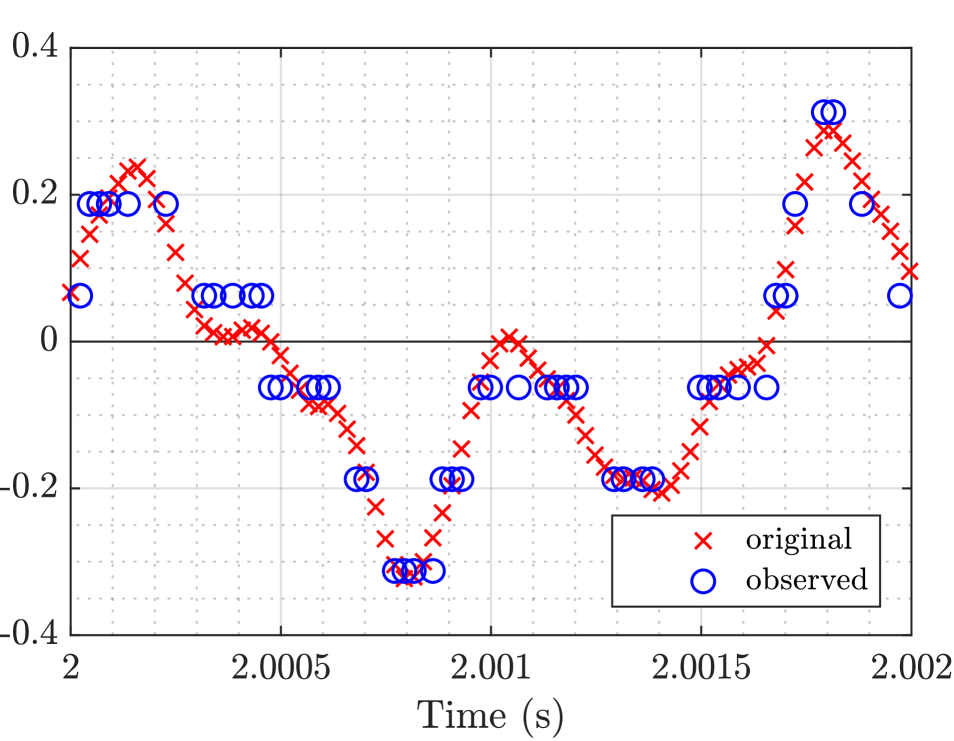
(a) piece of the subsampled and quantized signal

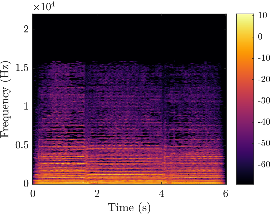
(b) spectrogram of the original signal

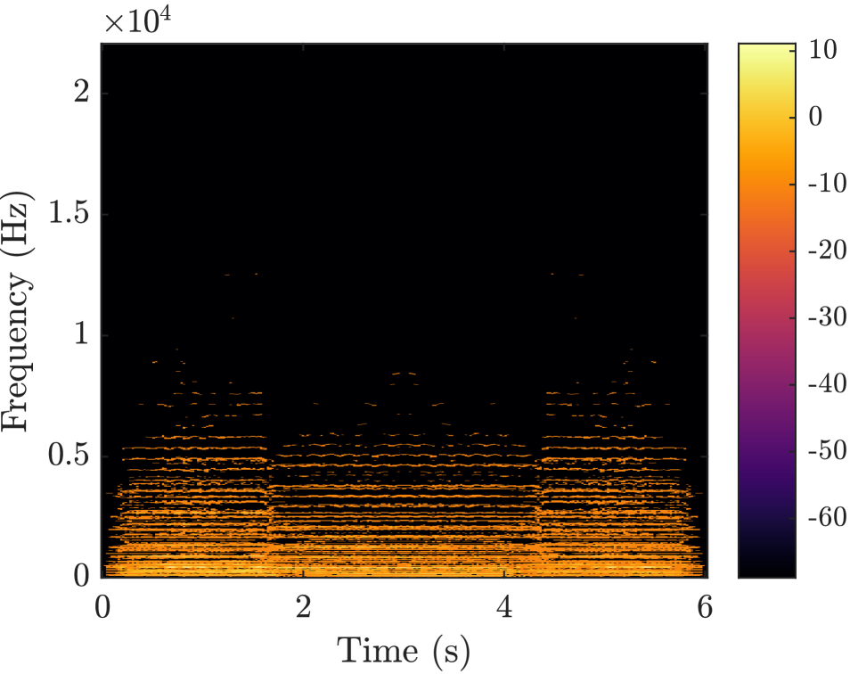
(c) spectrogram with kept quantized values

Figure 2: Data available to the decoder: (a) subsampled and quantized time-domain samples, and (c) subsampled and quantized TF coefficients. Although the real and imaginary parts are treated separately in the TF domain, the magnitude spectrogram is depicted here.

4.1 Design of the experiment

The task is to reconstruct a signal where some samples are missing; moreover, the retained samples are quantized. At the same time, a partial and quantized observation of the TF coefficients of the original (non-distorted) signal is provided. The goal is to illustrate that it is beneficial to utilize the double-domain approach, compared to the reconstruction using only information in the time domain (abbreviated to T domain in some of the figures). The relaxed sparse prior, i.e. the $\ell_{1}$ norm, is used, hence we can apply the consistent convex approach from Sec. 3.2.

The percentage of available samples/coefficients varies from $10\,\%$ up to $90\,\%$. It is denoted by $p_{\mathrm{T}}$ and $p_{\mathrm{TF}}$, respectively. In the time domain, the reliable samples are distributed (uniformly) randomly. In the TF domain, the coefficients that are the largest in magnitude are kept (Sec. 4.1.1 gives additional comments on the choice of the coefficients). The quantization is uniform and it is done by limiting the number of bits per sample ($b_{\mathrm{T}}$) or per coefficient ($b_{\mathrm{TF}}$). For a given bit depth $b$ (i.e. the number of bits used for representing each number), $\Delta=2^{-b+1}$ denotes the distance of two consecutive quantization levels. The quantized observation $u^{\mathrm{quant}}$ of a real value $u$, $-1\leq u\leq 1$ is obtained using the so-called mid-riser uniform quantizer [22] as

$$u^{\mathrm{quant}}=\operatorname{sgn}^{\!+}(u)\left(\left\lfloor\frac{\left|u\right|}{\Delta}\right\rfloor+\frac{1}{2}\right),$$ (18)

where $\operatorname{sgn}^{\!+}(u)$ returns 1 for $u\geq 0$ and $-1$ for $u<0$. The bit depths $b_{\mathrm{T}}$ and $b_{\mathrm{TF}}$ are chosen as the powers of two and they are equal, $b_{\mathrm{T}}=b_{\mathrm{TF}}\in\{2,4,8,16,32\}$. The samples or coefficients considered lost are the only exception, they are simply set to zero.

As the TF transform, the discrete Gabor transform (DGT) is used, with the sine window of 2048 samples in length, 50 % overlap and 2048 frequency channels. Such a transform produces a twice-redundant tight frame, which is then normalized to obtain a Parseval tight frame. As the prior, we use $\mathcal{S}\!=\!\|\cdot\|_{1}$ with no weighting, i.e. $W=\mathrm{Id}$.

For an illustrative scheme of the degradation, see Fig. 1. Fig. 2 then shows an example of the degraded signal and coefficients.

In order to evaluate the results, the PEMO-Q ODG score [29] and the SDR are measured, the latter being defined as

$$\mathrm{SDR}(\mathbf{y},\hat{\mathbf{y}})=10\log_{10}\frac{\|\mathbf{y}\|^{2}}{\|\mathbf{y}-\hat{\mathbf{y}}\|^{2}},$$ (19)

where $\mathbf{y}$ is the original (non-distorted) time-domain signal and $\hat{\mathbf{y}}$ is the reconstruction. The result is expressed in decibels. Unlike the SDR, PEMO-Q is a perceptually motivated measure whose ODG output score ranges from $-4$ (very annoying distortion, poor quality) to $0$ (imperceptible distortion, excellent quality).

The experiment is run for a set of 10 audio signals (musical recordings) of varying complexity from the SQAM database [30]. The signals are sampled at 44.1 kHz. To reduce the computational time due to the enormous number of tested combinations, the proof-of-concept experiment only uses one-second long excerpts. A single reconstruction instance then takes ca. 5 s, depending on the parameters of the computer. For the purpose of quantization, these excerpts are also peak-normalized such that the maximum absolute value of each signal equals one.

The CV algorithm 3 is executed setting $\tau=\sigma=\sqrt{2}/2$, $\rho=1$, and it stops after 300 iterations. The choice of $\tau$ and $\sigma$ follows from (14) and (16b), since $\|\sum_{m=1}^{2}L_{m}^{*}L_{m}\|=\|K^{*}K+K^{*}K\|=2\|K^{*}K\|=2$ both in the synthesis case ($K=\mathrm{Id}$) and in the analysis case ($K=A$), assuming a Parseval tight frame and $W=\mathrm{Id}$.

4.1.1 On the choice and quantization of the TF coefficients

In the experiment, a tight Gabor frame is used to compute the TF representation of a real signal. Coefficients obtained using such a frame attain a specific complex-conjugate structure. In fact, only a half of all the coefficients are needed; the other half may be computed as a conjugate to the first half. Such a structure introduces a kind of redundancy: A pair of coefficients, given they are complex-conjugate, contribute to the total bit rate by the same amount as a pair of real samples of the signal. This property is used in the implementation when choosing the subset of the TF coefficients; it is ensured that for a given number of reliable samples or coefficients, information from the TF domain yields the same bit rate as information from the time domain.

Furthermore, recall that the quantization defined by Eq. (18) is tailored for values from the interval $[-1,1]$. To simulate the quantization for the observed TF coefficients $\mathbf{c}$, the quantization step $\Delta$ and all the quantization and decision levels in the TF domain are scaled by a factor of $\max\{\max\{\left|\Re(\mathbf{c})\right|\},\;\max\{\left|\Im(\mathbf{c})\right|\}\}$.

4.2 Results

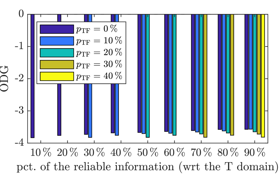
(a) ODG, synthesis model, 4 bits

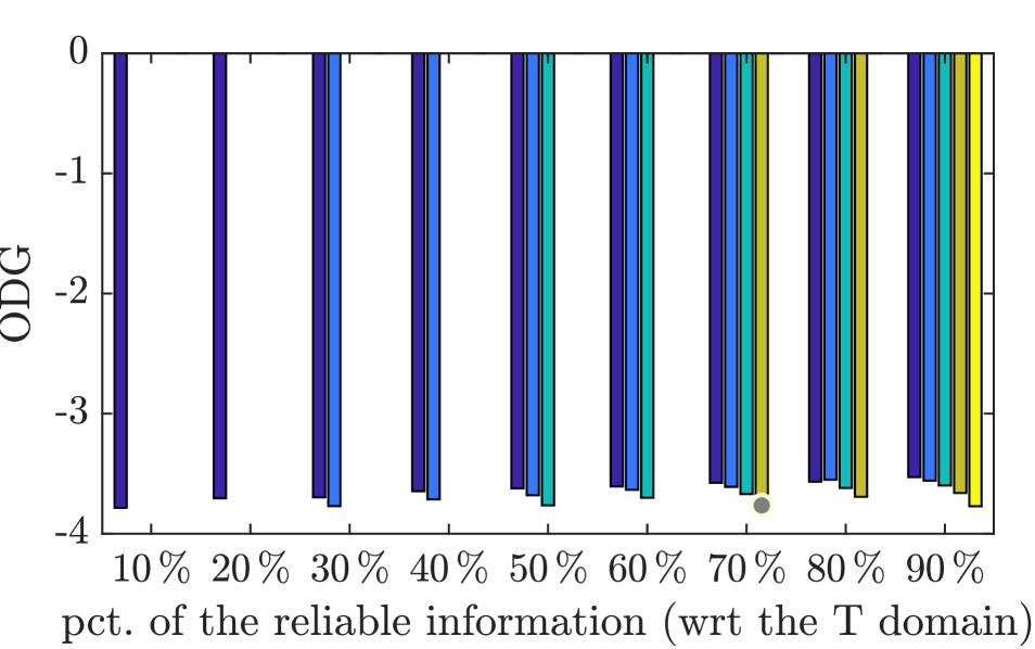
(b) ODG, analysis model, 4 bits

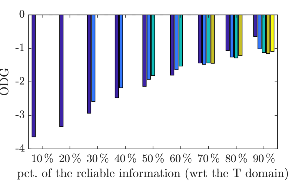
(c) ODG, analysis model, 16 bits

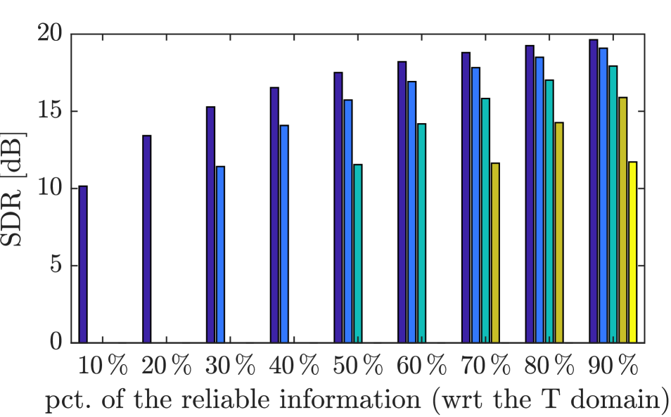
(d) SDR, synthesis model, 4 bits

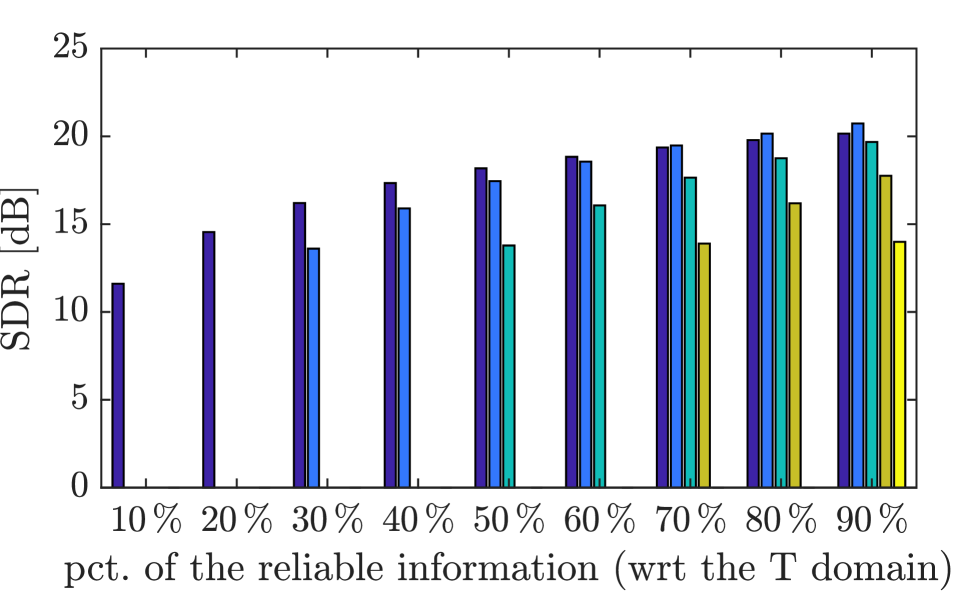
(e) SDR, analysis model, 4 bits

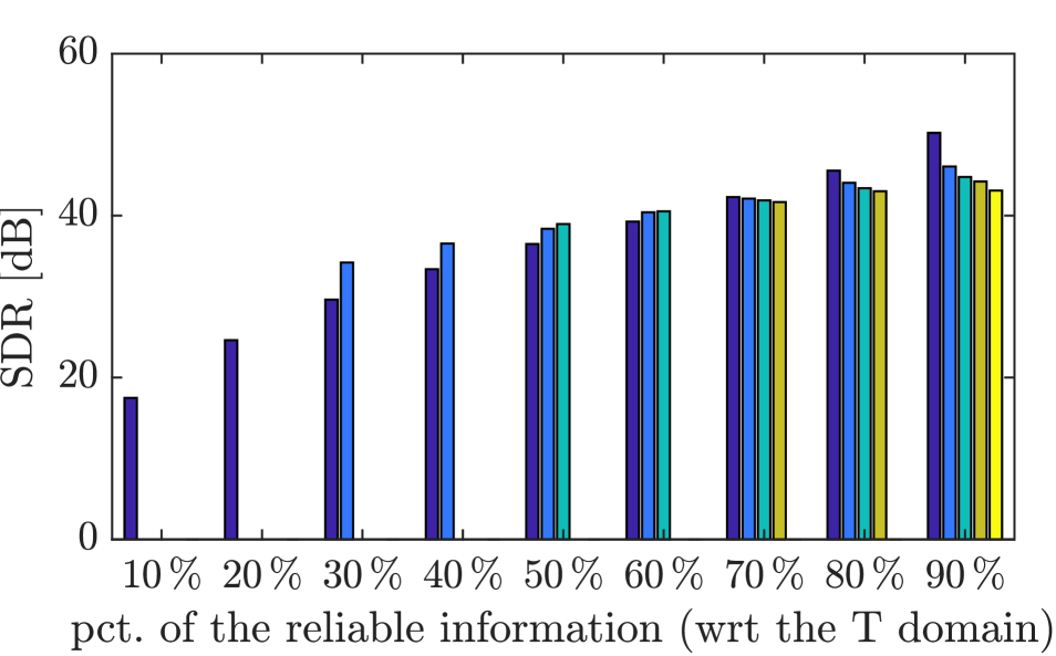
(f) SDR, analysis model, 16 bits

Figure 3: Comparison with fixed bit depth. The legend shown in the first plot is common to all the plots; $p_{\mathrm{TF}}$ denotes the percentage of reliable TF coefficients. Here, reliable coefficient means that it is observed (i.e. not missing), although it is quantized.

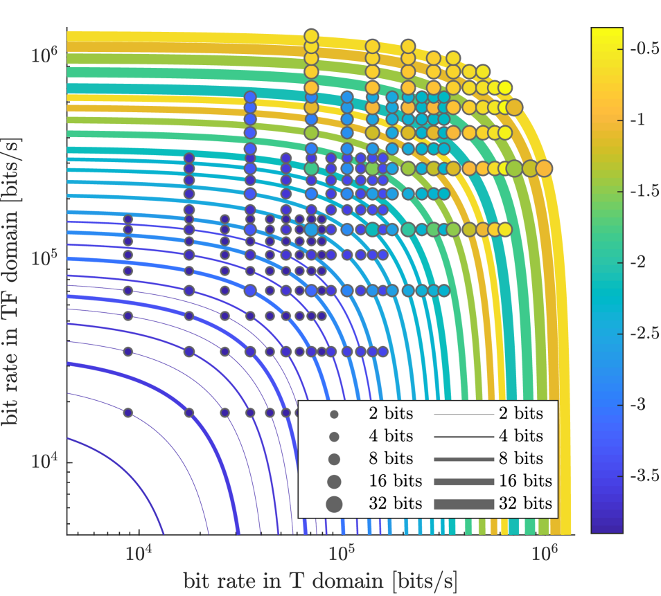
(a) ODG, analysis model

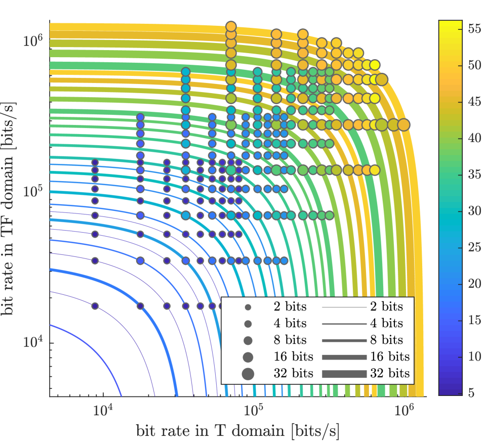
(b) SDR, analysis model

Figure 4: Comparison with variable bit depth. The bit rate is the quantity of bits per a second of audio.

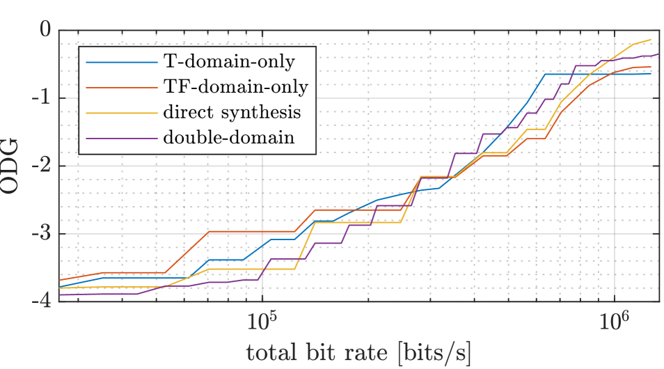
(a) ODG, analysis model

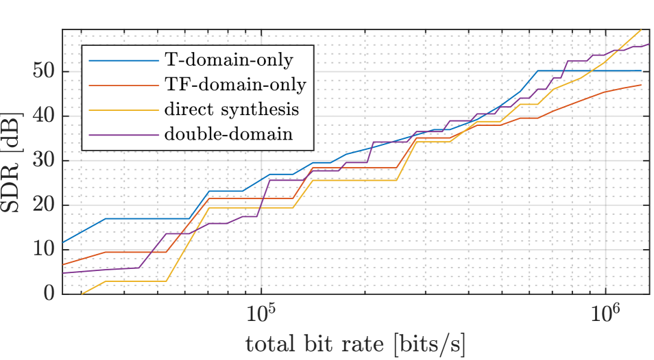
(b) SDR, analysis model

Figure 5: Comparison of the best performance of different approaches, given the limit of available total bit rate.

4.2.1 Comparison with fixed bit depth

All the results are visualized as mean values computed from the 10 audio signals. In the first visualization in Figure 3, the bit depth is fixed. The result corresponding to the T-domain-only approach (denoted by $p_{\mathrm{TF}}=0\,\%$) with a given fraction of reliable samples in the time domain serves as a reference. These two parameters—bit depth and fraction—define the bit rate of reliable information used in the T-domain-only approach. This reference scenario is compared to different distributions of the total amount of bits between the time and TF domains while using the previously fixed bit depth. Note that only a limited number of options of how to distribute the information between the time and the TF domains was tested.

Both evaluation metrics (ODG and SDR) are depicted in Fig. 3. For the bit depth $b_{\mathrm{T}}=b_{\mathrm{TF}}=4$, we present the results using both the analysis and the synthesis models (plots 3(a), 3(b), 3(d), 3(e)). Since no significant difference between the performance of the analysis and the synthesis approaches is observed, only the analysis model is used for further comparison with the performance using $b_{\mathrm{T}}=b_{\mathrm{TF}}=16$ (plots 3(c) and 3(f)).

For a fixed number of bits per sample or coefficient, it is in general not beneficial to split the available information between the two domains; see the decrease in both ODG and SDR in the plots 3(a), 3(b), 3(d) and 3(e) when the percentage of reliable TF coefficients increases. Sampling in the TF domain (in our setup) is reasonable only with a high bit depth—compare, for example, plots 3(e) and 3(f), where the difference is less significant.

4.2.2 Comparison with variable bit depth

In the visualization in Fig. 4, the number of bits per sample or coefficient varies. Two ways of displaying the results are combined in the figure.

The T-domain-only approach is represented by the colored equibital lines​. The line color represents the restoration quality, according to the side colorbar. The line width represents the bit depth and the position represents the bit rate (in this case, only time-domain information is used).

The double-domain approach is represented by the colored points. Once again, the color indicates the restoration quality. The point size represents the bit depth $b_{\mathrm{T}}=b_{\mathrm{TF}}$. Finally, the position represents the distribution of reliable information between the domains.

Both in the case of lines and in the case of points, the following rule is applied: If more realizations with the same bit distribution appear, only the best of them is plotted. Such a situation occurs when we decrease the number of reliable samples/coefficients while we increase the bit depth.

The scatter plots in Figure 4 show that there is a number of cases where it is useful to decrease the precision of the reliable time-domain samples and assign a part of the bit budget to the TF domain. This conclusion can be deduced from points which lie on an equibital line. Using the TF-domain information is advantageous when such a point reports a higher ODG/SDR compared to the line it lies on.

The evaluation is concluded by Fig. 5, which provides a different perspective to Fig. 4. The figure considers only the best performance in terms of ODG (Fig. 5(a)) or SDR (Fig. 5(b)) as a function of available total bit rate. In other words, it does not consider results in a situation when a higher bit rate does not lead to a better performance (cf. Fig. 4(a), the 5th and the 6th equibital from the top). The plots show that there are cases where the double-domain approach outperforms the T-domain-only approach, however, the difference is only minor. Significant gain is observed only for the highest bit rates, i.e. a low level of compression.

For the sake of completeness, the TF-domain-only reconstruction is included in Fig. 5 as well. In this case, the reconstruction is carried out based solely on partially observed and quantized TF coefficients. We consider two options: Either we follow the framework where the observation induces the set $\Gamma_{\mathrm{TF}}$, and Alg. 3 provides the reconstruction, or the quantized, partially observed coefficients are directly synthesized with $A^{*}$. Interestingly, both the T-domain-only and the double-domain approaches remain superior in great number cases; in particular regarding the SDR.

4.3 Software and reproducible research

The experiment was run in MATLAB R2019b, using LTFAT [31] version 2.3.1. All MATLAB codes, together with supplemental material, are provided in the repository at https://github.com/ondrejmokry/AudioRestorationFramework/.

5 Conclusion

The paper provides a general flexible formulation not only covering multiple audio reconstruction tasks, but also allowing several degradation types to take place simultaneously. Another novelty is that the restoration can possibly take into account constraints in the time-frequency domain. The concept can be easily extended such that the reliable information is distributed among more than two different transform domains. In Sec. 3.3, it is proposed how to develop the framework such that it handles noise-distorted data.

The aim of the experiment was not to outperform the state-of-the-art methods in the field of audio reconstruction, but to show an application of the general formulation in a meaningful audio compression scenario. The framework was shown to be flexible enough to cover a model of signal distortion which included both drop-outs and quantization of both the samples in the time domain and of the time-frequency coefficients. Although only a single scenario was considered, we observed promising results. It remains for the future work to find an optimal distribution of the bit budget between the time and the time-frequency domains.

6 Acknowledgments

The work was supported by the Czech Science Foundation (GAČR) project number 20-29009S. The authors thank the reviewers for their comments and suggestions, especially the reviewer number 4.

References

- [1] L. Rencker, F. Bach, W. Wang, and M. D. Plumbley, “Sparse recovery and dictionary learning from nonlinear compressive measurements,” IEEE Trans. Signal Processing, 2019.
- [2] C. Gaultier et al., “A modeling and algorithmic framework for (non)social (co)sparse audio restoration,” 2017, URL: https://arxiv.org/abs/1711.11259.
- [3] C. Gaultier, Design and evaluation of sparse models and algorithms for audio inverse problems, PhD thesis, Université Rennes 1, 2019.
- [4] Ç. Bilen, A. Ozerov, and P. Pérez, “Solving time-domain audio inverse problems using nonnegative tensor factorization,” IEEE Trans. Signal Processing, 2018.
- [5] A. Adler et al., “Audio Inpainting,” IEEE Trans. Audio, Speech, and Language Processing, 2012.
- [6] K. Siedenburg, M. Kowalski, and M. Dorfler, “Audio declipping with social sparsity,” in IEEE International Conference on Acoustics, Speech and Signal Processing. 2014.
- [7] O. Mokrý and P. Rajmic, “Reweighted minimization for audio inpainting,” in 2019 SPARS workshop, Toulouse.
- [8] P. Záviška et al., “Psychoacoustically motivated audio declipping based on weighted minimization,” in Int. Conf. on Telecommunications and Signal Processing, 2019.
- [9] S. Shlien, “Guide to MPEG-1 audio standard,” IEEE Trans. Broadcasting, 1994.
- [10] L. Jacques et al., “Dequantizing compressed sensing: When oversampling and non-gaussian constraints combine,” IEEE Trans. Information Theory, 2011.
- [11] P. Peter et al., “Compressing audio signals with inpainting-based sparsification,” in Scale Space and Variational Methods in Computer Vision, Springer, Cham, 2019.
- [12] K. Gröchenig, Foundations of time-frequency analysis, Birkhäuser, 2001.
- [13] P. Balazs et al., Frame Theory for Signal Processing in Psychoacoustics, Springer, Cham, 2017.
- [14] P. Záviška, P. Rajmic, Z. Průša, and V. Veselý, “Revisiting synthesis model in sparse audio declipper,” in Latent Variable Analysis and Signal Separation, Springer, Cham, 2018.
- [15] O. Derrien et al., “A quasi-orthogonal, invertible, and perceptually relevant time-frequency transform for audio coding,” in European Signal Processing Conference, 2015.
- [16] A. Janssen et al., “Adaptive interpolation of discrete-time signals that can be modeled as autoregressive processes,” IEEE Trans. Acoustics, Speech and Signal Processing, 1986.
- [17] W. Etter, “Restoration of a discrete-time signal segment by interpolation based on the left-sided and right-sided autoregressive parameters,” IEEE Trans. Signal Processing, 1996.
- [18] M. Lagrange, S. Marchand, and J.-B. Rault, “Long interpolation of audio signals using linear prediction in sinusoidal modeling,” Journal of the Audio Engineering Society, 2005.
- [19] O. Mokrý et al., “Introducing SPAIN (SParse Audio INpainter),” in European Signal Processing Conference. 2019.
- [20] C.-T. Tan et al., “The effect of nonlinear distortion on the perceived quality of music and speech signals,” Journal of the Audio Engineering Society, 2003.
- [21] J. Málek, “Blind compensation of memoryless nonlinear distortions in sparse signals,” in European Signal Processing Conference, 2013.
- [22] R. M. Gray and D. L. Neuhoff, “Quantization,” IEEE Trans. Information Theory, 1998.
- [23] D. L. Donoho and M. Elad, “Optimally sparse representation in general (nonorthogonal) dictionaries via minimization,” The National Academy of Sciences, 2003.
- [24] P. L. Combettes and J. C. Pesquet, “Proximal splitting methods in signal processing,” Fixed-Point Algorithms for Inverse Problems in Science and Engineering, 2011.
- [25] L. Condat, “A generic proximal algorithm for convex optimization—application to total variation minimization,” IEEE Signal Processing Letters, 2014.
- [26] B. C. Vũ, “A splitting algorithm for dual monotone inclusions involving cocoercive operators,” Advances in Computational Mathematics, 2011.
- [27] J. J. Moreau, “Proximité et dualité dans un espace hilbertien,” Bulletin de la société mathématique de France, 1965.
- [28] P. Rajmic et al., “A new generalized projection and its application to acceleration of audio declipping,” Axioms, 2019.
- [29] R. Huber and B. Kollmeier, “PEMO-Q—A new method for objective audio quality assessment using a model of auditory perception,” IEEE Trans. Audio Speech Language Processing, 2006.
- [30] “EBU SQAM CD: Sound quality assessment material recordings for subjective tests,” online, URL: https://tech.ebu.ch/publications/sqamcd.
- [31] Z. Průša et al., “The Large Time-Frequency Analysis Toolbox 2.0,” in Sound, Music, and Motion. Springer, 2014.