gBeam-ACO: a greedy and faster variant of Beam-ACO

Abstract

Beam-ACO, a modification of the traditional Ant Colony Optimization (ACO) algorithms that incorporates a modified beam search, is one of the most effective ACO algorithms for solving the Traveling Salesman Problem (TSP). Although adding beam search to the ACO heuristic search process is effective, it also increases the amount of work (in terms of partial paths) done by the algorithm at each step. In this work, we introduce a greedy variant of Beam-ACO that uses a greedy path selection heuristic. The exploitation of the greedy path selection is offset by the exploration required in maintaining the beam of paths. This approach has the added benefit of avoiding costly calls to a random number generator and reduces the algorithms internal state, making it simpler to parallelize. Our experiments demonstrate that not only is our greedy Beam-ACO (gBeam-ACO) faster than traditional Beam-ACO, in some cases by an order of magnitude, but it does not sacrifice quality of the found solution, especially on large TSP instances. We also found that our greedy algorithm, which we refer to as gBeam-ACO, was less dependent on hyperparameter settings.

Index terms— Ant Colony Optimization, Greedy Search, Beam-ACO

1 Introduction

Ant Colony Optimization (ACO) is an effective family of heuristic search algorithms for the traveling salesman problem (TSP) [1, 2]. The TSP is defined as finding the shortest path in a graph $G=(V,E,d)$, where $d(x,y)$ is a distance function,

$$d(x,y):V\times V\rightarrow\mathbb{R}$$

such that each vertex $v\in V$ is visited exactly once. The variant of the TSP [2] we use in this paper is the symmetric TSP in $\mathbb{R}^{2}$ that has the property $d(x,y)=d(y,x)$ $\forall x,y\in V$. We use the so-called Euclidean2D distance function, as defined in TSPLIB [3, 4], where distance is calculated as the rounded Euclidean distance between two points. That is

$$d(\mathbf{x},\mathbf{y})=\lfloor||\mathbf{x}-\mathbf{y}||_{2}+0.5\rfloor$$

Additionally, we assume a complete graph where each vertex is connected to every other vertex. Building a valid path in this graph involves selecting a sequence of $|V|-1$ nodes from a starting node (referred to as the depot) where there is an implicit connection from the last selected node to the depot. Finding the optimal solution to the TSP requires evaluating all $|V|!$ paths.

Ant Colony Optimization algorithms construct this path by traversing the graph using so-called ants and depositing so-called “pheromone” on the graph edges based on the characteristics of the traversed paths (e.g., shorter paths result in more pheromone). Pheromone levels on the edges of the graph encourage the ants to explore parts of the graph that have previously resulted in shorter paths.

ACO has a number of variants that mainly differ in the pheromone update rule. The original Ant System (AS) [5] updated the pheromone levels using the paths of all the ants in the colony. Elitist[6, 7] and Min-Max Ant System (MMAS) [8] are two of the most popular variants. The Elitist ACO variant is characterized by only updating the pheoromone levels with the shortest path traversed by the ant colony. MMAS, on the other hand, is similar to AS in that each ant’s path contributes to the pheromone update, but also scales pheromone levels such that they are guaranteed to be between user-specified minimum and maximum levels.

One particularly effective variant of ACO is Beam-ACO [9, 10, 11, 12, 13] , which adapts Beam search [14, 15] to the ACO algorithm. As with other ACO implementations, Beam-ACO relies on a pseudo-random number generator (PRNG). PRNGs can be very performant, such as the PCG family of PRNGs [16]; however, they are frequently a bottleneck in stochastic algorithms. For example, prior work on particle swarm optimization noted that the way in which the random numbers were generated for use by the algorithm had a material impact on performance [17]. Stochastic algorithms require additional thought when parallelizing because the PRNG may represent shared state, which can cause contention when called from multiple threads. This is can be overcome using techniques such as using thread-local PRNG functions or a producer-consumer approach with a thread-safe queue, but none of these are simpler than simply avoiding the need for a PRNG.

Greedy search heuristics are known to find sub-optimal solutions on many problems, one of which is the Traveling Salesman Problem. The typical greedy algorithm for the TSP is to select the shortest path to an unvisited vertex from the current vertex. This algorithm will select the same path each iteration without any exploration. We use the term iteration to mean one generation of a path or paths for all ants (in the case of ACO), followed by updating the pheromone matrix using an appropriate update rule.

Ant Colony Optimization algorithms use a heuristic function that combines edge length and pheromone level. The pheromone amounts change each iteration of the algorithm based on pheromone “evaporation” and pheromone deposits from the ants. This means there is no guarantee a greedily selected path one iteration will be the same as the greedily selected path from the previous iteration. In the initial stages of the algorithm, these paths may be quite different.

In this work, we propose a greedy variant of the Beam-ACO algorithm, referred to as gBeam-ACO, that replaces the stochastic beam search heuristic of Beam-ACO with a greedy approach. The primary motivation of this approach is to avoid costly operations associated with PRNGs. We show that replacing the stochastic heuristic with a greedy heuristic improves runtime performance by more than 50% while still maintaining the quality of solutions. The trade-off with this approach, as with all greedy heuristics, is the algorithm focuses more on exploitation rather than exploration. This means the beam-width hyper-parameter of the Beam-ACO algorithm is important because it gives the algorithm some degree of exploration. This greedy approach works in the ACO setting because heuristic weights of the paths are updated during the initial phases of the search. Thus, although the algorithm is greedy, it is likely that it will not visit the same paths until the pheromone matrix has stabilized.

2 Prior Work

Most similar to our work is that of Beam-ACO [9, 10, 11, 12, 13]. Our work differs from the original by proposing the use of a greedy heuristic during beam selection rather than using a stochastic heuristic. This results in an improved runtime, which consequently leads to better found solutions for the same running time and iteration count.

Application of a greedy heuristic to ACO was explored in [18, 19]. Vendramin et al. propose a greedy variant of the ACO heuristic as a routing protocol in delay tolerant networks. They use an event-based mechanism to decay pheromones, which is is an important difference to our work. In our work we want pheromone levels to decay at each time step to ensure we don’t get stuck in a sub-optimal path. As proposed in [9], using an MMAS-style pheromone update rule means every feasible path remains feasible because there is always a non-zero pheromone level. Additionally, our use of beam search means we are less likely to get stuck in a sub-optimal solution resulting from a greedy path extension since we consider a number of partial paths simultaneously.

Greedy ACO algorithms have also been studied in the design of wide sensor networks [20] and networking [21]. In this setting, the idea is to prefer vertices that have a larger number of neighboring vertices within range of their network. While this is technically a greedy heuristic (greedy in the number of reachable neighbors), it has the effect of increasing exploration rather than increasing exploitation, which is the usual effect of choosing a greedy algorithm. In this sense, the approach is very different from our work. We are not choosing vertices based on their number of neighbors; because we are working on a complete graph this heuristic is not effective. Additionally, we focus solely on the pheromone heuristic to guide the search. Our algorithm focuses on exploring the top-$k$ most promising paths (for beam width $k$) as defined by the ACO heuristic function.

While there are some works that apply greedy modifications to ACO in the context of the Traveling Salesman Problem, most work involving greedy algorithms are for more classical search techniques. For example, [22] applies a greedy selection algorithm with an adaptive simulated annealing [23] algorithm.

3 Beam-ACO

The combination of beam search with ACO was introduced in [9] and described by Algorithm 1. ACO iteratively constructs solutions by randomly sampling from the distribution of heuristic weights, described in Algorithm 2, probabilistically guided by heuristic information [24]. The heuristic function used by ACO is the weighted product of the reciprocal of the edge length and the current pheromone level of the respective edge. This is shown equation (1), where $\alpha$ and $\beta$ are constants chosen by the user, $P(x,y)$ is the pheromone level on the edge connecting node $x$ and node $y$, and $E(x,y)$ is the length of the edge between $x$ and $y$.

$$h(x,y)=P(x,y)^{\alpha}E(x,y)^{\beta}$$ (1)

We use $\alpha=1$ and $\beta=4$, based on the analysis from [25] but note that the optimal values of these parameters is highly problem dependent. Anecdotaly, we found these values of $\alpha$ and $\beta$ produced better results for all ACO algorithms in our experiments than using $\alpha=1$ and $\beta=1$. Beam-ACO selects the edge stochastically by normalizing the heuristic weights for each edge and setting $h(x,y)$ to $0$ if $y$ has already been visited. The probability distribution used by Beam-ACO for selecting a new vertex $y$ is given by equation (2), where $V$ is the set of vertices of the graph $G=(V,E)$ for the respective TSP and $P$ is the set of previously visited vertices.

$$p(y|x)=\begin{cases}0&y\in P\\ h(x,y)/\sum_{y^{\prime}\in V\setminus P}h(x,y^{\prime})&\text{otherwise}\end{cases}$$ (2)

Note that the current vertex is considered visited, which means there is no chance of selecting the current vertex. Beam-ACO incorporates a probabilistic beam search to expand partial solutions for each ant. Prior work on beam search [26] noted that it is particularly effective for large problems and we observed this in our experiments. Although both Beam-ACO and gBeam-ACO found better solutions than both Elitist and MMAS, the gap widened quite dramatically as the TSP instance size grew. Define $k_{\text{ext}}$ as the number of extensions (i.e., generated partial solutions) from the current vertex and define $k_{\text{bw}}$ as the beam width (i.e., the number of partial solutions maintained between iterations). This differs somewhat from classical Beam search in that we restrict the exploration to $k_{\text{ext}}$ rather than explore the entire frontier, which consists of all unvisited nodes. This reduces exploration but also improves runtime efficiency. In our algorithm we set $k_{\text{ext}}=k_{\text{bw}}$ and refer to the common value as the beam width, denoted by $k$. Paths are pruned based their current length.

Algorithm 1 Beam-ACO algorithm.

1:procedure Beam-ACO($G,n_{\text{search}},n_{\text{paths}},p(s,i)$)

2:     $G$ - TSP graph

3:     $n_{\text{search}}$ – # of beam search candidates

4:     $n_{\text{paths}}$ – # of maintained paths

5:     $p(s)$ – predicate that specifies when to stop searching

6:     $\mathcal{S}\leftarrow\emptyset$ – candidate solutions, $|\mathcal{S}|\leq n_{\text{ants}}$

7:     $\texttt{i}\leftarrow 0$$\triangleright$ Current iteration.

8:     // Repeat until stopping predicate it true

9:     while not $p(\mathcal{S},\texttt{i})$ do

10:         $\texttt{i}\leftarrow\texttt{i}+1$

11:         for $s\in\mathcal{S}$ do

12:              // Extended solution stochastically or greedily

13:              $\mathcal{S}\leftarrow\mathcal{S}\cup\texttt{ExtendAcoSolution}(s,k,G,\texttt{SolutionType})$

14:         end for

15:         $n\leftarrow\min(n_{\text{paths}},|\mathcal{S}|)$

16:         $\mathcal{S}\leftarrow\texttt{PickTopN}(\mathcal{S},n)$

17:         $G.\texttt{pheromones}\leftarrow\texttt{PheromoneUpdateRule}(\mathcal{S},G)$

18:     end while

19:     return $\arg\min_{s\in S}||s||$

20:end procedure

21:procedure ExtendAcoSolution($s,G,\texttt{SolutionType}$)

22:     SolutionType - an enum of either STOCHASTIC or GREEDY

23:     if SolutionType is STOCHASTIC then

24:         return StochasticExtendAcoSolution(s, k, G)

25:     else

26:         return GreedyExtendAcoSolution(s, k, G)

27:     end if

28:end procedure

Algorithm 2 Stochastic extension of partial ACO solution.

1:procedure StochasticExtendAcoSoltuion($s,k,G$)

2:     $s$ – current partial solution

3:     $G$ – graph data structure containing distances and pheromone

4:     $G.\texttt{pheromones}$ – the pheromone matrix

5:     $\mathcal{S}\leftarrow\emptyset$ – new partial paths levels

6:     // Most recently added node in candidate solution.

7:     $n\leftarrow s.\texttt{currentNode}$

8:     for $i=1$ t $k$ do

9:         //$+$ operator is clone and append

10:         $\mathcal{S}\leftarrow\mathcal{S}\cup s+\texttt{RandomSample}(G.\texttt{pheromones}[n])$

11:     end for

12:     return $\mathcal{S}$

13:end procedure

We found Beam-ACO to be an effective ACO algorithm, returning better results than both Elitist and MMAS ACO algorithms. As discussed in greater detail in Section 4, Beam-ACO does more work per iteration than the standard ACO algorithms, which means Beam-ACO cannot be compared with these standard ACO algorithms on a per-iteration basis.

The reason Beam-ACO is so effective with respect to other ACO algorithms is that the beam search component forces the algorithm to explore a larger number of partial paths. For a single ant in a typical ACO algorithm, a path is constructed probabilistically vertex by vertex. A Beam-ACO ant with beam width of $k$ will select $k$ vertices for each partial path it is constructing. This means after the first step it will consider a total of $k^{2}$ paths and select the $k$ shortest of those paths. Compared to a colony of $n$ ants running a standard ACO algorithm, a Beam-ACO ant will explore a much larger variety of partial paths. This is why Beam-ACO is so effective at finding better solutions than the typical ACO algorithms, but it is also why we must be careful in our performance measurements. We want to make sure we compare algorithms when they are doing equivalent amounts of work.

3.1 Greedy Beam-ACO

Modifying the Beam-ACO algorithm for a greedy heuristic is very straightforward: instead of sampling during the path construction section of the algorithm (Algorithm 2, line 10) we simply select the $k$ paths with the largest heuristic weights for a beam-width of $k$. The full description of the gBeam-ACO algorithm is the same as that shown in Algorithm 1, except we replace the ExtendAcoSolution call with the GreedyExtendAcoSolution procedure described in Algorithm 3. This is done by passing an enum as one of the arguments to ExtendAcoSolution, which can take on the values SolutionType.STOCHASTIC or SolutionType.GREEDY.

There are a two motivations for using this greedy approach over a stochastic selection algorithm. First, we can improve runtime performance by avoiding calls to a PRNG without using a complex alternative, such as using a buffered channel to communicate random numbers generated in a separate thread. Secondly, because we are greedily selecting based on the heuristic edge weight $h(x,y)$, and $h(x,y)$ changes each iteration, we force selection and evaluation of the $k$ most promising paths for the current iteration. Maintaining the beam in this setting helps the algorithm overcome some of the exploitation-bias.

There is extensive prior work benchmarking and improving runtime performance and parallelization of PRNGs [27, 28, 29]. Despite this progress, skipping the call to the PRNG will always be faster (i.e., no work is better than some work). There is always a trade-off and in this case it is in the quality of the solution. As we will demonstrate experimentally, on average gBeam-ACO’s solutions are within 5% of Beam-ACO’s solutions (and occassionally better than Beam-ACO) but it finds these solutions nearly an order of magnitude faster than Beam-ACO. We found that avoiding the PRNG alone was worth about an 8-10% performance boost.

One interesting consequence of using a greedy selection algorithm when constructing the path is that every ant will construct the same set of partial paths and return the same final path. Table 1 shows this consequence: “gBeam-10x1” is gBeam-ACO with a beam width of 10 and 1 ant while “gBeam-10x10” is gBeam-ACO with a beam width of 10 and 10 ants, both have identical path length numbers. This means there is no benefit to using more than one ant, which means that gBeam-ACO, when compared with Beam-ACO using $n$ ants, should at least see around a $(n-1)/n$ reduction in its runtime simply from only having to maintain a single ant. This consequence is where gBeam-ACO gets the majority of its runtime performance improvement. It is also interesting to note that despite only using a single ant with a greedy path construction heuristic it is able to find similar quality solutions to standard Beam-ACO using multiple ants.

gBeam-ACO finds high quality solutions using a greedy heuristic in a problem setting where greedy algorithms typically struggle because it has a guaranteed level of exploration from maintaining the beam of partial solutions. Additionally, the pheromone levels change each iteration, leading to new greedily constructed solutions. The changing pheromone levels make it less likely that a greedily constructed path resulting in a poor solution will be constructed again because the pheromones on the edges of the respective path will all decrease before the next iteration. While the changing pheromone levels help gBeam-ACO explore the graph, maintaining the search beam is the key aspect of the algorithm that offsets the exploitation-bias of the greedy path construction heuristic. During partial path construction, a gBeam-ACO ant will explore $k$ new partial paths for each of its current $k$ partial paths. This means for a beam width of $k=10$, each partial path extension step will consider 100 new partial paths and then prune them down to the 10 shortest. A corresponding Beam-ACO ant will do the same exploration, but also make 100 calls to a PRNG. Additionally, Beam-ACO will repeat this 10 times generating 1,000 new and unique partial paths and pruning them down to 100 (10 partial paths per ant). Given the disparity in work between the two algorithms, it is somewhat surprising that gBeam-ACO is able to find solutions of similar quality.

Algorithm 3 Greedy extension of partial ACO solution.

1:procedure GreedyExtendAcoSolution($s,k,G$)

2:     $s$ – current partial solution

3:     $k$ – beam width

4:     $G$ – Data structure storing TSP and ACO metadata

5:     $S\leftarrow\emptyset$ $\triangleright$ Empty set to store partial paths

6:     $n\leftarrow s.\texttt{currentNode}$ $\triangleright$ Most recently added node in candidate solution.

7:     $\texttt{minNode}\leftarrow\texttt{FindMaxNotInSet}(n.\texttt{neighbors},-\infty$)

8:     for $i=1$ to $k$ do

9:         $\texttt{minNode}\leftarrow\texttt{FindMaxNotInSet}(n.\texttt{neighbors},\texttt{minNode}$)

10:         $S\leftarrow S\cup s.\texttt{cloneAndAppend(minNode)}$

11:     end for

12:     return $S$

13:end procedure

Algorithm 4 Max-finding algorithm: finds $\max xs\setminus ys$.

1:procedure FindMaxNotInSet($xs,ys$)

2:     $xs$ - collection of TSP node indices

3:     $ys$ - set of previously selected indices

4:     $x^{\prime}\leftarrow xs[0]$ $\triangleright$ Set to initial element

5:     $w^{\prime}\leftarrow\texttt{HeuristicWeight}(x^{\prime})$

6:     for $x\in xs$ do

7:         $w^{\prime}\leftarrow\texttt{HeuristicWeight}(x)$

8:         if $w^{\prime}>w\textbf{ and }x^{\prime}\not\in ys$ then

9:              $(x^{\prime},w^{\prime})\leftarrow(x,w)$

10:         end if

11:     end for

12:     $\textbf{return }x^{\prime}$

13:end procedure

3.2 Complexity

Suppose we have $n$ ants, a beam width of $k$, and a TSP with $|V|$ vertices. The ACO algorithm will consider $O(n|V|^{2})$ partial paths per iteration while the Beam-ACO algorithm will consider $O(n|V|^{2}k^{2})$ partial paths. The gBeam-ACO iteration complexity is slightly different from Beam-ACO because it only needs a single ant and its greedy update rule, which takes $O(|V|k)$ time. Thus the gBeam-ACO complexity is given by $O(|V|^{2}k^{2})$.

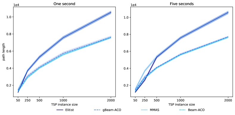
Figure 1: Comparison of ACO algorithms for varying durations.

3.3 Trade-offs

The major trade-off is exploration – gBeam-ACO is an exploitation-heavy algorithm, which means it will favor paths it knows are promising over exploring new paths that may be less promising or do not have much heuristic information. As previously discussed, because the heuristic weights change each iteration and the algorithm maintains a beam of partial paths, there is a level of forced exploration.

The other issue with the exploitation versus exploration trade-off is that once the pheromone distribution has converged to a stable distribution after some number of iterations, gBeam-ACO will always produce the same set of solutions–which may or may not be optimal–while Beam-ACO is capable of producing new, previously unexplored solutions. We note that both Beam-ACO and gBeam-ACO are computationally intense ACO algorithms, both of which do substantially more work per iteration than vanilla ACO algorithms. In our experience, both gBeam-ACO and Beam-ACO are about $30-50\times$ slower on a per iteration basis for TSP instances with 500 to 1,000 vertices. In other words, the gBeam-ACO and Beam-ACO algorithms were only able to complete one or two iterations in the same time vanilla ACO algorithms such as Elitist Ant System [7, 6] and Max-Min Ant System (MMAS) [8] were able to complete 30 to 50 iterations. Despite the difference in iteration count, gBeam-ACO and Beam-ACO produced dramatically better solutions. The large amount of per-iteration work performed by gBeam-ACO means it will take a relatively long time (in terms of wall clock time) for gBeam-ACO’s pheromone distribution to converge to a fixed distribution. It is important to note that gBeam-ACO seems to be very effective even when it is only run for one or two iterations.

4 Results

In our initial work it became apparent that gBeam-ACO was able to achieve similar results to standard Beam-ACO but in a much shorter time. Care must be taken in these measurements because these algorithms are doing a different amount of work per iteration. As an example, comparing ACO with Beam-ACO on a per-iteration basis is not a fair comparison because they consider different numbers of partial paths per iteration. Similarly, we must be careful in measuring the differences between Beam-ACO and gBeam-ACO because gBeam-ACO only uses a single ant, which means at minimum it will do $n-1$ fewer iterations than Beam-ACO. This makes a fair comparison rather difficult because gBeam-ACO is doing less work for a fixed iteration count (because there are fewer ants) but because it has a shorter wall-clock runtime when compared to Beam-ACO it is able to do more iterations per fixed unit of time.

All experiments use the same hyper-parameter tunings. We set $\alpha=1$ and $\beta=4$. Pheromones evaporate at a rate of $0.1$ and the pheromone deposit amount is $1.0$. MMAS min and max pheromone levels are 0.1 and 0.9, respectively. Experiments that use randomly generated TSP instances use the domain $[-100,100]\times[-100,100]$.

Figure 1 compares Elitist, MMAS, Beam-ACO, and gBeam-ACO on a fixed duration basis. Fifteen TSP instances were randomly generated and evaluated by each of the algorithms. All algorithms ran for approximately one and five seconds. We did not stop algorithms mid-iteration. This was not an issue for TSP instances 500 vertices and smaller, but for the 1,000 and 2,000 vertex instances both gBeam-ACO and Beam-ACO ran longer than the allotted time. In both of these cases gBeam-ACO and Beam-ACO only completed a single iteration while Elitist and MMAS both completed on the order of tens of iterations. This gives some insight as to the value of maintaining the search beam – despite both gBeam-ACO and Beam-ACO not being able to take advantage of the updated pheromone matrix, both were able to find better solutions than Elitist and MMAS algorithms. Both gBeam-ACO and Beam-ACO outperform Elitist and MMAS algorithms on larger problem size. Because the main difference in the algorithms is the beam search component, this matches previous observations on beam search [26] that it performs particularly well on large problem sizes. Although it is interesting that Elitist finds the best solutions for the 50 and 250 size problems while running for five seconds, we don’t find this particularly damaging to the Beam-ACO family of algorithms because these are relatively small TSP instances.

Figure 2 shows the results of the fixed iteration experiment. This experiment compares Beam-ACO and gBeam-ACO on a per iteration basis. We do not track runtime because gBeam-ACO has a major advantage. Rather, we are interested in how the quality of their solutions differ given that one algorithm is doing more work than the other. These experiments are performed on 15 randomly generated TSP instances. Two aspects of Figure 2 stand out: gBeam-ACO finds solutions that are comparable (although not better) to Beam-ACO and as the problem size grows this difference becomes smaller. This matches intuition — Beam-ACO performs more exploration than gBeam-ACO, so we would expect it to consider a more diverse population of paths (that is, paths that may not appear as promising based purely on their heuristic weigh). This diversity means it may find paths that gBeam-ACO would never consider because of its greedy selection heuristic.

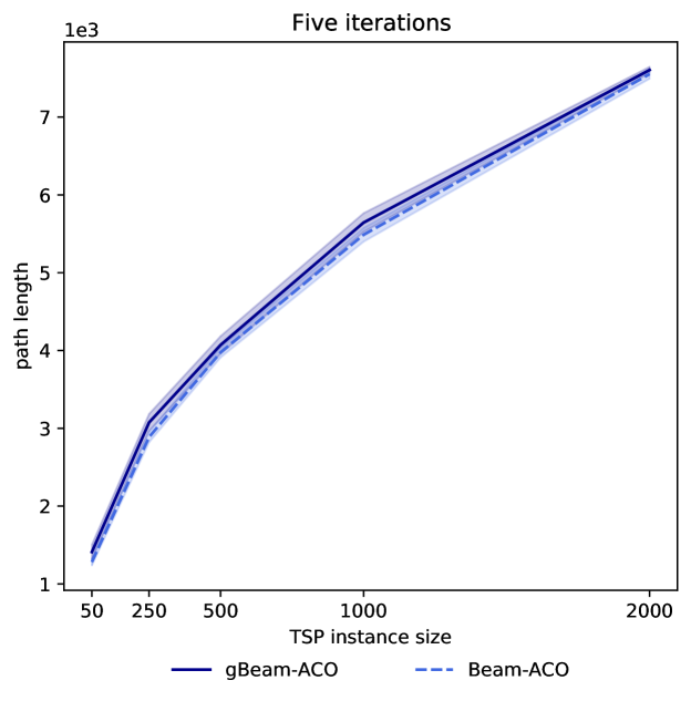
Figure 2: Comparison of best found path length for the same number of iterations.

To address the total work disparity, we perform another set of experiments where a third gBeam-ACO instance whose beam width, $k_{\text{equiv}}$ is set using equation (3), where $n$ and $k$ are taken from a Beam-ACO instance.

$$k_{\text{equiv}}=\frac{\sqrt{n}}{k}$$ (3)

This gBeam-ACO instance attempts to do a similar amount of work as a given Beam-ACO instance. This work largely comes from the partial path extensions performed when expanding the beam. For example, if Beam-ACO has 10 ants using a beam width of 10, then each ant is exploring 100 partial paths, or 1,000 partial paths in total. Using equation (3) yields a beam width of about 32, which leads to 1,024 partial paths explored at each step by a single ant. Thus, gBeam-ACO with a beam width of 32 should perform roughly the same amount of work as Beam-ACO with 10 ants and a beam width of 10.

Table 1 shows the results of this experiment, and also includes a gBeam-ACO instance with 10 ants with a beam width of 10. This last instance was included to confirm the claim that running gBeam-ACO with more than one ant is unnecessary. These results are based on 10 randomly generated TSP instances. Each algorithm in this experiment performs five iterations.

The most notable result in this table is that gBeam-ACO with a single ant is over 90% faster than Beam-ACO while finding paths that are, on average, less than 5% longer. In other words, gBeam-ACO trades a 5% decrease in quality of solution for a 90% increase in speed. Comparing gBeam-ACO with 10 ants to Beam-ACO shows over a 10% reduction in runtime almost across the board. This runtime savings is purely from avoiding calls to the PRNG. This comes at a cost — Beam-ACO is able to consistently find shorter paths than gBeam-ACO due to gBeam-ACO’s bias towards exploitation over exploration.

Another interesting and somewhat surprising result is the performance of gBeam-ACO with a beam width of 32 and a single ant. As expected from equation  (3), the runtime is similar to Beam-ACO. Our expectation was that the wider beam would result in better solutions when compared to a smaller beam width gBeam-ACO algorithm and possibly better solutions than standard Beam-ACO. Although the solutions of the $k=32$ beam width are better than $k=10$, we were surprised that they were not that much better, especially given the runtime differences. Perhaps what is more surprising is that the wider beam width gBeam-ACO was not able to consistently find better solutions than Beam-ACO. This illustrates the importance of exploration in finding better solutions.

Table 1: Comparison of several variants of gBeam-ACO with Beam-ACO based on 10 trials of randomly generated TSP instances.

Path Length Runtime TSP Size Beam-10x10 gBeam-10x1 gBeam-32x1 gBeam-10x10 Beam-10x10 gBeam-10x1 gBeam-32x1 gBeam-10x10 50 $\mathbf{1,449\pm 98}$ $1,513\pm 107$ $1,446\pm 69$ $1,513\pm 107$ $0.69\pm 0.02$ $\mathbf{0.07\pm 0.00}$ $0.66\pm 0.01$ $0.72\pm 0.01$ 250 $\mathbf{2,859\pm 98}$ $3,052\pm 97$ $3,082\pm 156$ $3,052\pm 97$ $16.63\pm 0.27$ $\mathbf{1.54\pm 0.03}$ $16.45\pm 0.20$ $15.42\pm 0.36$ 500 $\mathbf{3,961\pm 87}$ $4,131\pm 89$ $4,129\pm 129$ $4,131\pm 89$ $68.31\pm 1.70$ $\mathbf{6.14\pm 0.19}$ $65.07\pm 1.64$ $61.29\pm 1.83$ 1,000 $\mathbf{5,528\pm 87}$ $5,670\pm 80$ $5,639\pm 101$ $5,670\pm 80$ $262.41\pm 5.73$ $\mathbf{22.74\pm 0.43}$ $240.25\pm 4.96$ $229.61\pm 5.84$

Table 2 compares Elitist and MMAS ACO algorithms against Beam-ACO and gBeam-ACO on 10 TSP instances taken from TSPLIB. Again, comparison between these algorithms is challenging because they perform different amounts of work per iteration. Beam-ACO has the largest per-iteration runtime cost, so we structured the runs of Elitist and MMAS ACO algorithms such that they would run for a similar wall-clock time as Beam-ACO. We restricted gBeam-ACO to either one second of runtime or a single iteration, whichever takes longer. This puts gBeam-ACO at a disadvantage in terms of quality of solution because gBeam-ACO is running for a tenth of the time of the other algorithms (excluding the first three instances), but as the results show gBeam-ACO still performs surprisingly well given these restrictions.

Of the ten TSP instances, gBeam-ACO found the best solution in 30% of the time, Beam-ACO found the best solution 50% of the time, and Elitist ACO found the best solution 20% of the time. Across the board, gBeam-ACO consistently had runtimes that were over 90% shorter than Beam-ACO’s runtime due to only using a single ant and avoiding PRNG calls. Recall that gBeam-ACO was restricted to run for either a second or a single iteration depending on which takes longer. If the runtime is over a few seconds that indicates that gBeam-ACO took longer than a second to complete a single iteration. Because gBeam-ACO has a dramatically shorter per-iteration runtime compared to Beam-ACO, we can infer that Beam-ACO only completed a single iteration in these settings as well. For these problems–every problem except a280, ch130, and ch150–gBeam-ACO was nearly 10 times faster than Beam-ACO. For these same problems, gBeam-ACO found the best solution three out of seven times and was within about 1% of the best found solution (found by Beam-ACO) for three of the remaining four problems (fnl4461, rl1323, rl5915, u2319).

Table 2: Results from TSP instances selected from TSPlib.

Path Length Runtime (s) 1,000 Partial Paths / s TSP Instance Elitist MMAS Beam gBeam Elitist MMAS Beam gBeam Elitist MMAS Beam gBeam a280 3,276 4,327 3,254 3,399 5.0 5.0 4.3 1.2 75 75 64 65 ch130 6,671 9,149 7,505 7,712 2.0 2.0 1.9 1.0 159 158 131 132 ch150 7,748 10,956 8,419 8,450 2.0 2.0 1.3 1.0 136 137 114 117 d1291 84,995 92,803 60,859 59,434 88.6 88.0 87.6 7.9 16 16 14 16 d1655 99,258 115,400 78,804 78,783 146.4 146.9 145.8 12.9 12 12 11 12 fnl4461 313,311 348,401 237,062 241,913 1,087.5 1,093.2 1,084.1 92.1 4 4 4 5 rl1304 474,377 501,293 336,368 357,146 87.2 87.4 86.4 7.1 17 17 15 18 rl1323 497,934 525,898 360,502 362,975 89.7 89.3 88.6 7.2 16 16 15 18 rl5915 1,140,250 1,183,545 754,365 765,015 1,883.9 1,888.3 1,876.2 143.8 3 3 3 4 u2319 396,029 420,631 292,107 291,531 275.3 276.1 273.1 23.0 9 9 8 10

5 Conclusion

We have introduced a greedy alternative to Beam-ACO and have demonstrated its effectiveness in a number of settings. gBeam-ACO is able to achieve comparable results (generally within 5% of Beam-ACO in our experiments) in a fraction of the time. There are two avenues of future work based on these promising results: (1) exploring a hybrid algorithm that uses gBeam-ACO to quickly find good solutions and uses standard Beam-ACO to fully explore those solutions and (2) exploring an asynchronous gBeam-ACO implementation where ants continuously share pheromone updates, which would allow gBeam-ACO to take advantage of larger colony sizes. gBeam-ACO’s performance make it a great option for exploratory analysis or bootstrapping pheromone matrices for other algorithms.

References

- [1] Gerhard Reinelt. The Traveling Salesman, Computational Solutions for TSP Applications, volume 840 of Lecture Notes in Computer Science. Springer, 1994.
- [2] Gregory Gutin and Abraham P Punnen. The traveling salesman problem and its variations, volume 12. Springer Science & Business Media, 2006.
- [3] Gerhard Reinelt. Tsplib.
- [4] Gerhard Reinelt. TSPLIB - A traveling salesman problem library. INFORMS J. Comput., 3(4):376–384, 1991.
- [5] Marco Dorigo. Optimization, learning and natural algorithms [ph. d. thesis]. Politecnico di Milano, Italy, 1992.
- [6] Ghaith M. Jaradat and Masri Ayob. An elitist-ant system for solving the post-enrolment course timetabling problem. In Yanchun Zhang, Alfredo Cuzzocrea, Jianhua Ma, Kyo-Il Chung, Tughrul Arslan, and Xiaofeng Song, editors, Database Theory and Application, Bio-Science and Bio-Technology - International Conferences, DTA and BSBT 2010, Held as Part of the Future Generation Information Technology Conference, FGIT 2010, Jeju Island, Korea, December 13-15, 2010. Proceedings, volume 118 of Communications in Computer and Information Science, pages 167–176. Springer, 2010.
- [7] Ayan Acharya, Deepyaman Maiti, Aritra Banerjee, and Amit Konar. Balancing exploration and exploitation by an elitist ant system with exponential pheromone deposition rule. CoRR, abs/0811.0131, 2008.
- [8] Thomas Stutzle and Holger H. Hoos. Max-min ant system. Future Gener. Comput. Syst., 16(9):889–914, June 2000.
- [9] Christian Blum. Beam-aco – hybridizing ant colony optimization with beam search: An application to open shop scheduling. Computers & Operations Research, 32(6):1565–1591, 2005.
- [10] Manuel López-Ibáñez and Christian Blum. Beam-aco for the travelling salesman problem with time windows. Computers & operations research, 37(9):1570–1583, 2010.
- [11] Christian Blum. Beam-aco for simple assembly line balancing. INFORMS Journal on Computing, 20(4):618–627, 2008.
- [12] Joao L Caldeira, Ricardo C Azevedo, Carlos A Silva, and Joao MC Sousa. Supply-chain management using aco and beam-aco algorithms. In 2007 IEEE International Fuzzy Systems Conference, pages 1–6. IEEE, 2007.
- [13] Dhananjay Thiruvady, Christian Blum, Bernd Meyer, and Andreas Ernst. Hybridizing beam-aco with constraint programming for single machine job scheduling. In International Workshop on Hybrid Metaheuristics, pages 30–44. Springer, 2009.
- [14] Mark F. Medress, Franklin S. Cooper, James W. Forgie, C. C. Green, Dennis H. Klatt, Michael H. O’Malley, Edward P. Neuburg, Allen Newell, Raj Reddy, H. Barry Ritea, J. E. Shoup-Hummel, Donald E. Walker, and William A. Woods. Speech understanding systems. Artif. Intell., 9(3):307–316, 1977.
- [15] Weixiong Zhang. Complete anytime beam search. In AAAI/IAAI, pages 425–430, 1998.
- [16] Melissa E. O’Neill. Pcg: A family of simple fast space-efficient statistically good algorithms for random number generation. Technical Report HMC-CS-2014-0905, Harvey Mudd College, Claremont, CA, September 2014.
- [17] Jeffrey Hajewski and Suely Oliveira. Two simple tricks for fast cache-aware parallel particle swarm optimization. In IEEE Congress on Evolutionary Computation, CEC 2019, Wellington, New Zealand, June 10-13, 2019, pages 1374–1381. IEEE, 2019.
- [18] Ana Cristina B. Kochem Vendramin, Anelise Munaretto, Myriam Regattieri Delgado, and Aline Carneiro Viana. A greedy ant colony optimization for routing in delay tolerant networks. In Workshops Proceedings of the Global Communications Conference, GLOBECOM 2011, 5-9 December 2011, Houston, Texas, USA, pages 1127–1132. IEEE, 2011.
- [19] Ana Cristina Kochem Vendramin, Anelise Munaretto, Myriam Regattieri Delgado, and Aline Carneiro Viana. Grant: Inferring best forwarders from complex networks’ dynamics through a greedy ant colony optimization. Computer Networks, 56(3):997 – 1015, 2012. (1) Complex Dynamic Networks (2) P2P Network Measurement.
- [20] Xuxun Liu and Desi He. Ant colony optimization with greedy migration mechanism for node deployment in wireless sensor networks. J. Netw. Comput. Appl., 39:310–318, 2014.
- [21] LI Chengming, LIU Wenjing, and Koji Okamura. A greedy ant colony forwarding algorithm for named data networking. Proceedings of the Asia-Pacific advanced network, 34:17–26, 2013.
- [22] Xiutang Geng, Zhihua Chen, Wei Yang, Deqian Shi, and Kai Zhao. Solving the traveling salesman problem based on an adaptive simulated annealing algorithm with greedy search. Applied Soft Computing, 11(4):3680 – 3689, 2011.
- [23] S. Kirkpatrick, C. D. Gelatt, and M. P. Vecchi. Optimization by simulated annealing. SCIENCE, 220(4598):671–680, 1983.
- [24] Marco Dorigo, Directeur de Recherches Du Fnrs Marco, Thomas Stützle, et al. Ant Colony Optimization. MIT Press, 2004.
- [25] Dorian Gaertner and Keith L. Clark. On optimal parameters for ant colony optimization algorithms. In Hamid R. Arabnia and Rose Joshua, editors, Proceedings of the 2005 International Conference on Artificial Intelligence, ICAI 2005, Las Vegas, Nevada, USA, June 27-30, 2005, Volume 1, pages 83–89. CSREA Press, 2005.
- [26] Christopher Makoto Wilt, Jordan Tyler Thayer, and Wheeler Ruml. A comparison of greedy search algorithms. In third annual symposium on combinatorial search, 2010.
- [27] Michael Mascagni and Ashok Srinivasan. Algorithm 806: Sprng: A scalable library for pseudorandom number generation. ACM Transactions on Mathematical Software (TOMS), 26(3):436–461, 2000.
- [28] A De Matteis and Simonetta Pagnutti. Parallelization of random number generators and long-range correlations. Numerische Mathematik, 53(5):595–608, 1988.
- [29] Paul D Coddington. Random number generators for parallel computers. 1997.