On Bayesian Search for the Feasible Space
Under Computationally Expensive Constraints

Abstract

We are often interested in identifying the feasible subset of a decision space under multiple constraints to permit effective design exploration. If determining feasibility required computationally expensive simulations, the cost of exploration would be prohibitive. Bayesian search is data-efficient for such problems: starting from a small dataset, the central concept is to use Bayesian models of constraints with an acquisition function to locate promising solutions that may improve predictions of feasibility when the dataset is augmented. At the end of this sequential active learning approach with a limited number of expensive evaluations, the models can accurately predict the feasibility of any solution obviating the need for full simulations. In this paper, we propose a novel acquisition function that combines the probability that a solution lies at the boundary between feasible and infeasible spaces (representing exploitation) and the entropy in predictions (representing exploration). Experiments confirmed the efficacy of the proposed function.

1 Introduction

In engineering applications, we are often interested in determining the feasible design space for a given problem. This requires estimating a set of decision variables that does not violate given conditions. This is a challenging task, particularly if the constraints cannot be expressed analytically. In these cases, computationally expensive simulations or physical experiments are required to explore the design space. For instance, in some nuclear power applications, keeping the neutron production ratio below a critical level is essential for safe operation [chevalier:fast]. This presents a significant design challenge without analytical constraints. It is not practical to test each set of plant parameters by simulation, since each evaluation of the simulator takes between $5$ and $30$ minutes. Hence, a classifier that can accurately predict feasibility can allow operators to explore the design space rapidly before setting up the plant obviating the need for simulations. The challenge is then how to train this classifier with few expensive evaluations.

In this context, surrogate-assisted Bayesian search method has been shown to be a data-efficient approach [knudde:active]. This method starts with a small training set of independent parameters. These parameters are expensively evaluated with a set of constraint functions. The resulting dataset is used to train a Bayesian regression model (in this case, a Gaussian process, $\mathcal{G}\mathcal{P}$) for each constraint [rasmussen:gpml]. Together, these models estimate the probability that a given solution is feasible. In this way, the combination of models act as a binary classifier. The idea is then to locate a candidate sample for evaluating expensively such that adding this sample to the training dataset would achieve the greatest improvement in the feasible space estimation. This candidate is located by maximising an acquisition function (often referred to as an infill criterion or a utility function). We keep adding new samples until the budget on additional expensive evaluations is exhausted.

We understand that using this method of Bayesian search for feasible region identification and design exploration is new with Knudde et al. publishing the first acquisition function recently [knudde:active]. This function considers the loss of entropy of the posterior predictive distribution from adding a new sample in the training dataset. With the aim of providing alternative acquisition functions, the novel contributions of this paper are:

• A new acquisition function $\alpha_{PBE}(\cdot)$ based on the probability of a solution residing at the boundary (representing exploitation) and the entropy of predictive distribution (representing exploration).

• Adaptation of a range of alternative acquisition functions (that are originally used in reliability engineering for rapidly estimating the volume of the infeasible space) for the purpose of data-efficient construction of a feasibility classifier.

• A full investigation of these acquisition functions in a set of constrained problems.

In section 2, we discuss necessary concepts focusing on using $\mathcal{G}\mathcal{P}$s to model constraints functions, and the standard Bayesian search framework. Then we propose a range of acquisition functions suitable for Bayesian search of the feasible space in section 3. We present our results in section 4. Finally, we finish with general conclusions in section 5.

2 Background

Consider, a design vector $\mathbf{x}$ in a design space $\mathcal{X}\in\mathbb{R}^{n}$. Without loss of generality, a constrained problem with $L$ constraints can be defined as:

$$G(\mathbf{x})=(g_{1}(\mathbf{x}),\dots,g_{L}(\mathbf{x}))^{\top}\leq\mathbf{t}=(t_{1},\dots,t_{L})^{\top},$$ (1)

where, $g_{l}:\mathbb{R}^{n}\rightarrow\mathbb{R}$ is the $l$th constraint function with a threshold for feasibility $t_{l}$. To deal with equality constraints, we can add a small fixed constant $\epsilon$. This converts the equation to an inequality constraint [cec2006].

The $l$th constraint function $g_{l}(\mathbf{x})$ generates a feasible space $\mathcal{F}_{l}\subseteq\mathcal{X}$. The infeasible set of solutions for this constraint is therefore $\mathcal{I}_{l}=\mathcal{X}\setminus\mathcal{F}_{l}$. The total infeasible set of solutions becomes $\mathcal{I}=\bigcup_{l=1}^{L}\mathcal{I}_{l}$. If all constraints are considered, the feasible space is at the intersection of all feasible sets: $\mathcal{F}=\bigcap_{l=1}^{L}\mathcal{F}_{l}$.

If constraint functions are cheap to evaluate, we can determine feasibility by brute force using Monte Carlo methods [mori:mcs]. However, where each constraint function evaluation $g_{l}(\mathbf{x})$ requires a computationally expensive simulation, this approach would be prohibitively slow.

2.1 Modelling Constraints with Gaussian Processes

Gaussian processes ($\mathcal{G}\mathcal{P}$) are commonly used to construct surrogate models for constraints $g_{l}(\mathbf{x})$. $\mathcal{G}\mathcal{P}$s produce a Normal predictive distribution for any arbitrary solution, producing a mean and standard deviation.

In essence, a $\mathcal{G}\mathcal{P}~{}$is a field of joint Gaussian distributions [rasmussen:gpml]. Consider a $\mathcal{G}\mathcal{P}~{}$trained for $l$th constraint function $g_{l}(\mathbf{x})$ on dataset $\mathcal{D}_{l}=\{(\mathbf{x}_{m},g_{l}(\mathbf{x}_{m}))\}_{m=1}^{M}$ evaluated at $M$ locations. The predictive probability for $g_{l}$ at $\mathbf{x}$ is a Gaussian distribution with mean $\mu_{l}(\mathbf{x})$ and variance $\sigma_{l}^{2}(\mathbf{x})$ is:

$$p(g_{l}~{}|~{}\mathbf{x},\mathcal{D}_{l})=\mathcal{N}(\mu_{l}(\mathbf{x}),\sigma_{l}^{2}(\mathbf{x})~{}|~{}\mathbf{x},\mathcal{D}_{l}).$$ (2)

The efficacy of $\mathcal{G}\mathcal{P}$s is conferred by a flexible kernel function. We use a Matern $5/2$ kernel, as recommended for modelling realistic functions [snoek:practical]. We refer the reader to [rasmussen:gpml] for full documentation on how the $\mathcal{G}\mathcal{P}~{}$is trained and interrogated.

We train a model for each constraint independently. Thus, the combined posterior predictive distribution across all component models is a multi-variate Gaussian:

$$p(G~{}|~{}\mathbf{x},\mathcal{D})=\mathcal{N}(\boldsymbol{\mu}(\mathbf{x}),\Sigma(\mathbf{x}))=\prod_{l=1}^{L}p(g_{l}~{}|~{}\mathbf{x},\mathcal{D}_{l}),$$ (3)

where, the training dataset is $\mathcal{D}=\{(\mathbf{x}_{m},g_{1}(\mathbf{x}_{m})),\dots,g_{L}(\mathbf{x}_{m}))\}_{m=1}^{M}$, the mean prediction vector is $\boldsymbol{\mu}(\mathbf{x})=(\mu_{1}(\mathbf{x}),\dots,\mu_{L}(\mathbf{x}))^{\top}$, and the predictive covariance matrix is $\Sigma(\mathbf{x})=\operatorname{diag}(\sigma^{2}_{1}(\mathbf{x}),\dots,\sigma^{2}_{L}(\mathbf{x}))$. There are no cross-covariances as each model is independent.

2.2 Classifying the Feasible Space

Since the predictive distribution is Gaussian, we can compute the probability of violation of each constraint. For the $l$th constraint, the probability of feasibility is [hughes:pdom, fieldsend:pdom, chevalier:kriginv]:

$$p(\mathbf{x}\in\mathcal{F}_{l})=p(~{}p(g_{l}~{}|~{}\mathbf{x},\mathcal{D}_{l})\leq t_{l}~{})=\Phi(\tau_{l}),$$ (4)

where $\tau_{l}=\frac{t_{l}-\mu_{l}(\mathbf{x})}{\sigma_{l}(\mathbf{x})}$ and $\Phi(\cdot)$ is the standard Gaussian cumulative distribution function. The overall probability of feasibility is therefore:

$$p(\mathbf{x}\in\mathcal{F})=\prod_{l=1}^{L}p(\mathbf{x}\in\mathcal{F}_{l})=\prod_{l=1}^{L}\Phi(\tau_{l}).$$ (5)

Due to symmetry, the probability of infeasibility is $p(\mathbf{x}\in\mathcal{I})=1-p(\mathbf{x}\in\mathcal{F})$. Using these probabilistic estimations, a decision vector $\mathbf{x}$ is feasible iff $p(\mathbf{x}\in\mathcal{F})>p(\mathbf{x}\in\mathcal{I})$. Figure 1 illustrates the predicted feasible spaces for two constraints modelled with two $\mathcal{G}\mathcal{P}$s.

Figure 1: Illustration of probability of feasibility (dotted red line) with two surrogate $\mathcal{G}\mathcal{P}$s trained on observations at regular intervals (depicted by black squares). The grey shaded areas represent the true feasible space due to the threshold vector $\mathbf{t}=(t_{1},t_{2})^{\top}=(0.05,1.5)^{\top}$ on constraint functions $g_{1}(\mathbf{x})=\sin(\mathbf{x})$ and $g_{2}(\mathbf{x})=2\sin(\mathbf{x}-1)$. The shaded areas around the mean predictions $\mu_{l}(\mathbf{x})$ (blue for $\mu_{1}(\mathbf{x})$ and green for $\mu_{2}(\mathbf{x})$) show the uncertainty estimations $2\sigma_{l}(\mathbf{x})$ from respective $\mathcal{G}\mathcal{P}$s. With only a few carefully selected observations, the models have well approximated the feasible space. In this paper, instead of sampling at regular intervals, our aim is to sequentially select the training data to construct the best possible classifier of feasibility with the smallest budget of expensive evaluations.

2.3 Bayesian Search Framework

Bayesian search is a surrogate-assisted active learning framework. This method takes inspiration from Efficient Global Optimisation (EGO), first proposed by Kushner [kushner:ego] and later improved by Jones et al. [jones:ego]. The framework can be used to minimise the mean squared error in the sequential design of experiments, and is particularly useful where there are few observations [sacks:design]. It has also been used to compute the volume of infeasible space [bect:sequential, chevalier:fast, chevalier:kriginv], and to locate the feasible space under multiple constraints [knudde:active].

Bayesian search is a global search strategy. It sequentially samples the design space to determine the boundary of the feasible space. The algorithm has two stages: initial sampling, and sequential improvement.

During the first stage, we sample the parameters using a space filling design, typically with Latin Hypercube sampling (LHS) [mckay:lhs]. These parameters are then evaluated by the true function. The LHS parameter samples and their true-function output create the initial training set. Each design set is used to create a set of models, one for each constraint, $\hat{G}=\{\hat{g}_{1},\dots,\hat{g}_{L}\}$.

For the sequential improvement phase, we can use $\hat{G}$ to locate promising samples. For an arbitrary design vector $\mathbf{x}$, the function $\hat{G}$ provides a multi-dimensional posterior distribution $p(G~{}|~{}\mathbf{x},\mathcal{D})$ with a mean prediction (a vector) and uncertainty (a covariance matrix). The predictive distribution permits a closed form calculation of probability. We use this predictive distribution to estimate the likelihood that a constraint function value will exceed a threshold. Since our goal is to minimise the uncertainty around the threshold that bounds the infeasible space, we can design our acquisition function $\alpha(\mathbf{x},\hat{G},\mathbf{t})$ accordingly. The aim is to strike a balance between exploitation (through the probability of a solution residing at the boundary) and global exploration (through the prediction uncertainty). In this way, the acquisition function will drive the search towards the areas we are interested in. The proposed acquisition functions are presented in section 3.

The most promising solution is defined where $\mathbf{x}^{*}=\operatorname*{\arg\!\max}_{\mathbf{x}}\alpha(\mathbf{x},\hat{G},\mathbf{t})$. We then determine $\mathbf{x}^{*}$ expensively, and use the results to augment the data and retrain $\hat{G}$. We repeat this process until we exhaust the simulation budget. When training is complete, we use $\hat{G}$ to estimate the feasible space. For an arbitrary $\mathbf{x}$ a probability of feasibility is returned using (5). Algorithm 1 summarises the method.

Algorithm 1 Bayesian search framework.

Inputs

$M:$ Number of initial samples

$T:$ Budget on expensive function evaluations

$\mathbf{t}:$ Threshold vector

Steps

1:$X\leftarrow\operatorname{LatinHypercubeSampling}(\mathcal{X})$ $\triangleright$ Generate initial samples

2:$\Gamma\leftarrow\{G(\mathbf{x}\in X)\}$ $\triangleright$ Expensively evaluate all initial samples

3:for $i=M\rightarrow T$ do

4:    $\hat{G}\leftarrow$ Train$\mathcal{G}\mathcal{P}$s$(X,\Gamma)$ $\triangleright$ Train a mono- or multi-surrogate model of constraints

5:    $\mathbf{x}^{*}\leftarrow\operatorname*{\arg\!\max}_{\mathbf{x}}\alpha(\mathbf{x},\hat{G},\mathbf{t})$ $\triangleright$ Optimise acquisition function

6:    $X\leftarrow X\cup\{\mathbf{x}^{*}\}$ $\triangleright$ Augment data set with $\mathbf{x}^{*}$

7:    $\Gamma\leftarrow\Gamma\cup\{G(\mathbf{x}^{*})\}$ $\triangleright$ Expensively evaluate $\mathbf{x}^{*}$

8:end for

9:return $\hat{G}$ $\triangleright$ Return trained models for feasibility classification using (5)

3 Acquisition Functions

For Bayesian search of the feasible space, the acquisition function’s aim is to locate the boundary between feasible and infeasible spaces: $\mathcal{F}_{l}$ and $\mathcal{I}_{l}$. A solution based on $\hat{g}_{l}$ is often identified with the probability of being at the boundary: $p(\mathbf{x}\in\mathcal{F}_{l})p(\mathbf{x}\in\mathcal{I}_{l})$. If we add the sample at this to the training set, the estimation of feasibility with $\hat{g}_{l}$ is maximally improved. In this way, we achieve maximal exploitation of the latest knowledge of the model.

When data is limited, the uncertainty in predictions may be high, especially in areas of the design space that have a sparse number of samples. We should, therefore, promote the exploration of these areas.

However, if we only prioritise sparsely populated areas, we may miss areas near the threshold of interest. We therefore need to consider areas where both the uncertainty and the boundary probability are high. We test both a range of existing and a novel acquisition function for balancing the above requirements.

The first acquisition function for feasible region discovery was proposed by Knudde et al. [knudde:active]. It is designed to maximise the loss in entropy of the posterior distribution around the boundary for adding a solution to the training dataset. For $l$th constraint, it can be expressed as:

$$\alpha_{K[l]}(\mathbf{x},\hat{g}_{l},t_{l})=\frac{1}{2}\ln(2\pi e\sigma_{l}^{2}(\mathbf{x}))-\ln(\Phi(\tau_{l})(1-\Phi(\tau_{l}))).$$ (6)

A detailed simplification of this equation is provided in the supplementary materials.

Here, the first term is the predictive entropy $\operatorname{\mathbb{H}}(p(g_{l}~{}|~{}\mathbf{x},\mathcal{D}))$ (representing areas of high uncertainty where exploration should be maximised). The second term is the natural logarithm of the probability of being at the boundary (representing exploitation of the knowledge of the boundary); c.f. equation (5).

This function was originally designed for a single constraint. For multiple constraints, they proposed to combine these component utilities across all constraints as a sum:

$$\alpha_{K}(\mathbf{x},\hat{G},\mathbf{t})=\sum_{l=1}^{L}\alpha_{K[l]}(\mathbf{x},\hat{g},t_{l}).$$ (7)

The summation formulation of the acquisition function permits a situation where one of the components $\alpha_{K[l]}$ can dominate the overall utility. For instance, if an arbitrary solution $\mathbf{x}$ is expected to gain significantly more information than other constraints, it may still maximise the acquisition utility and thus get evaluated. This biases the search towards maximal individual gain without allowing existing information to influence over the value of the acquisition function. As a result, the overall progress of this acquisition function may be slow.

We also adapt a range of alternative acquisition functions from the field of reliability engineering. These acquisition functions were originally developed for a single constraint, and were first used in an active learning framework by Ranjan et al. [ranjan:single] and Bichon et al. [bichon:single], and later popularised by Picheny et al. [picheny:single, chevalier:fast] for computing the volume of the infeasible space.

The most popular acquisition functions for single constraint are:

$$\alpha_{T[l]}(\mathbf{x},\hat{g}_{l},t_{l}) =\sigma(\mathbf{x})\phi(z),$$ (8)

$$\alpha_{B[l]}(\mathbf{x},\hat{g}_{l},t_{l}) =\sigma(\mathbf{x})[z^{+}\Phi(z^{+})+z^{-}\Phi(z^{-})+\phi(z^{+})+\phi(z^{-})-2z\Phi(z)-2\phi(z)],$$ (9)

$$\alpha_{R[l]}(\mathbf{x},\hat{g}_{l},t_{l}) =\sigma^{2}(\mathbf{x})[z^{2}(\Phi(z^{-})-\Phi(z^{+}))+z^{+}\phi(z^{-})-z^{-}\phi(z^{+})].$$ (10)

Here, $z=\frac{\mu_{l}(\mathbf{x})-t_{l}}{\sigma(\mathbf{x})}$, $z^{+}=z+1$, $z^{-}=z-1$, and $\phi(\cdot)$ is the standard Gaussian probability density function. $\alpha_{T[l]}(\cdot)$ is the targeted mean squared error and was defined by Picheny et al. [chevalier:kriginv]. $\alpha_{B[l]}(\cdot)$ and $\alpha_{R[l]}(\cdot)$ are functions that compute a form of average positive difference between uncertainty and the predictive distance from the threshold, defined by Bichon et al. [bichon:single] and Ranjan et al. [ranjan:single]. Further details of these can be found in [chevalier:kriginv, bect:sequential].

A similar acquisition function proposed by Echard et al. that can also be used [echard:ak]. This is written as [echard:ak, yang:system]:

$$\alpha_{E[l]}(\mathbf{x},\hat{g}_{l},t_{l})=-\frac{|\mu_{l}(\mathbf{x})-t_{l}|}{\sigma_{l}(\mathbf{x})}.$$ (11)

This is the negative of the probability of wrongly predicting feasibility. Maximising this function finds solutions that reduce the misclassification error.

To determine areas of system failure under multiple constraints, a composite-criterion approach is commonly taken. This approach calculates the acquisition function for each model, selecting a single model based on the best individual mean prediction [echard:ak, fauriat:ak, yang:system]. We reformulated this approach into a generalised version appropriate for Bayesian search (without requiring a large number of Monte Carlo samples):

$$\alpha_{Y}(\mathbf{x},\hat{G},\mathbf{t})=\alpha_{Y[k]}(\mathbf{x},\hat{g_{k}},t_{k})~{}|~{}k=\operatorname*{\arg\!\max}_{l=1}^{L}(\mu_{l}(\mathbf{x})-t_{l}),$$ (12)

where, $\alpha_{Y[k]}(\mathbf{x},\hat{g_{k}},t_{k})$ is the acquisition function for $k$th constraint $g_{k}(\mathbf{x})$, with $Y\in\{T,B,R,E\}$.

Using the acquisition function (12) improves the learning of the individual boundaries between feasible and infeasible spaces for each constraint $g_{k}(\mathbf{x})$. However, this approach does not directly account for the true boundary under multiple constraints. For multiple constraints, any violation is treated as infeasible, and since equation (12) may sample infeasible space, it will likely introduce unnecessary redundancy. A further weakness is that the model selection term $k=\operatorname*{\arg\!\max}_{l=1}^{L}(\mu_{l}(\mathbf{x})-t_{l})$ does not consider prediction uncertainty. The result can therefore be misleading. The scale of the function value in each constraint can also cause problems, since the magnitude differences in $\mu_{l}(\mathbf{x})-t_{l}$ may be inverse to relative importance. Our new acquisition function aims to solve these shortcomings.

3.1 Probability of Being at the Boundary and Entropy (PBE)

We have discussed how single-constraint acquisition functions can be combined to create an acquisition function for multiple constraints. However, since our aim is to find solutions with a high probability of being at the boundary of the feasible space (exploitation), whilst minimising the overall uncertainty in the models (exploration), we combine these two objectives as a product.

The probability that a solution is at the boundary $\beta$ between the feasible and infeasible spaces, given a multi-surrogate model $\hat{G}$, is:

$$p(\mathbf{x}\in\beta)=p(\mathbf{x}\in\mathcal{F})~{}p(\mathbf{x}\in\mathcal{I})=\prod_{l=1}^{L}\Phi(\tau_{l})-\prod_{l=1}^{L}\Phi^{2}(\tau_{l}).$$ (13)

If we maximise the probability over the design space, we will locate solutions at the boundary, thereby exploiting the current knowledge.

To evaluate the overall uncertainty for a multi-surrogate model $\hat{G}$, we compute the differential entropy of a multi-variate Gaussian distribution:

$$\operatorname{\mathbb{H}}(\mathbf{x}~{}|~{}\hat{G})=\frac{L}{2}\ln(2\pi e)+\frac{1}{2}\ln(|~{}\Sigma~{}|)\propto\ln\left(\prod_{l=1}^{L}\sigma^{2}_{l}(\mathbf{x})\right).$$ (14)

The extremes of the above equation identify the solutions with most overall uncertainty across the models. These extremes identify the most informative samples.

To maximise both quantities, we combine these two measures together as a product. This is a somewhat greedy approach that ensures that a solution that improves all components is selected. Our multi-surrogate acquisition function – the Probability of Boundary and Entropy (PBE) – is defined as:

$$\alpha_{PBE}(\mathbf{x},\hat{G},\mathbf{t})=p(\mathbf{x}\in\beta)~{}\operatorname{\mathbb{H}}(\mathbf{x}~{}|~{}\hat{G}).$$ (15)

This function addresses the true boundary $\beta$, which is at the intersection of all component constraints’ feasible spaces $\mathcal{F}=\bigcap_{l=1}^{L}\mathcal{F}_{l}$, directly. It is particularly useful, since no explicit model selection is required. Further, since the probability and entropy are being computed via an intra-constraint model (rather than between constraints), we expect it to perform better for unscaled function responses.

4 Experiments

To test the performance of our approach, we used the test suite for constrained single-objective optimisation problems from CEC2006 [cec2006].

We selected a range of problems with only non-linear inequality constraints (for simplicity) and varying proportional volume of the feasible space between $0.5\%$ and $45\%$ (Table 1). Note that we merely use these problems as example constrained problems for design exploration, and we do not seek to locate the global optimum.

Table 1: A range of test problems with a feasible space volume $\rho=\frac{|\mathcal{F}|}{|\mathcal{F}|+|\mathcal{I}|}\times 100\%\geq 0.5\%$ from the test suite defined in [cec2006] and implemented in PyGMO [pygmo]. Here, $n$ is the dimension of the decision space, and $L$ is the number of constraints.

ID	$n$	$\rho(\%)$	$L$
G4	5	26.9953	6
G8	2	0.8727	2
G9	7	0.5218	4
G19	15	33.4856	5
G24	2	44.2294	2

We ran each method starting from an initial sample size of $n$ where $n$ is the dimension of the decision space to avoid modelling an under-determined system. We set our budget on expensive evaluations to $11n$ to allow each method to gather $10n$ samples after initial sampling. This budget is less than the number of evaluations used by Knudde et al. [knudde:active] and Yang et al. (in reliability engineering) [yang:system] for reporting their results.

We ran each method on each problem $21$ times . The initial evaluations are matched between acquisition functions, i.e. for each pair of problem and simulation run, the same initial design was used. The exception to this is the LHS with $11n$ samples.

Since the acquisition function landscape is (typically) multi-modal, we used Bi-POP-CMA-ES to search the space, as it is known to solve multi-modal problems effectively [hansen:compare]. We set the maximum number of evaluations of the acquisition function to $5000n$.

We use informedness as a performance indicator for the classifier. The informedness estimates the probability that a prediction is informed, compared to a chance guess. We chose informedness (instead of F1 measure used in [knudde:active]) as it performs well for imbalanced class sizes, which are common when comparing the sizes of feasible and infeasible spaces for real-world constrained problems [powers:evaluation, tharwat:classification]. To ensure that we get an accurate estimation, we used $10000$ uniformly random samples from the decision space for validation. We keep these validation sets constant across different methods for a specific simulation number and a specific problem.

We used the one-sided Wilcoxon Signed Rank test with Bonferroni correction to test statistical equivalence to the best median performance, due to matched samples. We identify the best method at the level of $p\leq 0.05$ [knowles:tutorial]. We used Mann-Whitney-U test to compare the LHS to the other methods (Table 2). We provide box plots for performance comparison in the supplementary sections.

Table 2: Performance of different acquisition functions in terms of median informedness ($\%$) and the median absolute deviation from the median (MAD). The red cells show the best median performance, while the blue cells depict the equivalent methods to the best.

		LHS	$\alpha_{K}$	$\alpha_{T}$	$\alpha_{B}$	$\alpha_{R}$	$\alpha_{E}$	$\alpha_{PBE}$
G4	Median	$99.83\%$	$99.66\%$	$99.95\%$	$99.94\%$	$99.93\%$	$99.95\%$	$99.99\%$
	MAD	$7.9\times 10^{-4}$	$1.3\times 10^{-3}$	$2.7\times 10^{-4}$	$2.5\times 10^{-4}$	$4.3\times 10^{-4}$	$2.1\times 10^{-4}$	$3.6\times 10^{-4}$
G8	Median	$97.85\%$	$93.51\%$	$99.99\%$	$98.85\%$	$98.85\%$	$98.86\%$	$100\%$
	MAD	$1.4\times 10^{-2}$	$8.9\times 10^{-2}$	$6.0\times 10^{-3}$	$1.0\times 10^{-2}$	$1.0\times 10^{-2}$	$9.0\times 10^{-3}$	$5.9\times 10^{-3}$
G9	Median	$20.26\%$	$35\%$	$81.62\%$	$80.55\%$	$76.19\%$	$97.95\%$	$81.24\%$
	MAD	$2.0\times 10^{-1}$	$1.5\times 10^{-1}$	$1.7\times 10^{-1}$	$2.3\times 10^{-1}$	$2.5\times 10^{-1}$	$1.6\times 10^{-2}$	$5.6\times 10^{-2}$
G19	Median	$99.89\%$	$99.68\%$	$99.92\%$	$99.91\%$	$99.92\%$	$99.94\%$	$99.91\%$
	MAD	$4.0\times 10^{-4}$	$7.8\times 10^{-4}$	$2.7\times 10^{-4}$	$2.4\times 10^{-4}$	$2.1\times 10^{-4}$	$2.5\times 10^{-4}$	$2.6\times 10^{-4}$
G24	Median	$99.59\%$	$59.75\%$	$99.66\%$	$99.66\%$	$99.63\%$	$99.63\%$	$99.71\%$
	MAD	$1.4\times 10^{-3}$	$7.4\times 10^{-2}$	$1.1\times 10^{-3}$	$6.1\times 10^{-4}$	$8.5\times 10^{-4}$	$1.8\times 10^{-2}$	$3.9\times 10^{-4}$

The results show that the acquisition functions proposed in this paper outperform naive LHS and the acquisition function $\alpha_{K}$ proposed by Knudde et al. [knudde:active]. G9 has the worst median performance of $20.26\%$ for LHS, where the volume of the feasible space is extremely small (about $0.5218\%$). Here too $\alpha_{K}$ performs worse than our acquisition function $\alpha_{PBE}$. The acquisition function $\alpha_{E}$ from Echard et al. outperforms all other methods with a median informedness of $97.95\%$. In three out of the five problems, $\alpha_{PBE}$ achieves the best median performance, while $\alpha_{E}$ performs best in the rest of the problems. The best median for any problem is at least $97.95\%$ with small MAD, demonstrating the efficacy of the proposed and adapted methods over the current state-of-the-art.

5 Conclusions

This paper has examined the problem of feasible space identification for computationally expensive problems. We have demonstrated an active learning approach using Bayesian models (Bayesian search) and developed a range of acquisition functions for this purpose. Our experiments show that our proposed acquisition function for Bayesian search outperforms naive LHS, and the current state-of-the-art $\alpha_{K}$. We propose that future work focusses on batch Bayesian search when it is possible to evaluate multiple solutions in parallel.

Supplementary Materials

In the following supplementary sections, we present a range of related information that the readers may find useful.

1 Related Work in Reliability Engineering

The reliability engineering literature has much work devoted to system reliability analysis (SRA). SRA is applied when there are multiple failure modes in a system [bichon:sra], and Yang et al. [yang:system] provide a comprehensive review of work in this area. In these cases, a sequential search approach is adopted to constructing constraint models, which are then used to compute the probability of failure. Here, their ultimate goal is to estimate the total volume of the infeasible space or the excursion set [vazquez:pof].

The earliest approaches to modelling the boundary of the feasible space used either polynomials (typically first or second-order) [freudenthal:safety, rackwitz:structural, castillo:uncertainty] or support vector machines (SVMs) [hurtado:structural]. However, these approaches are limited. Under multiple constraints, the boundary is often highly-non-linear, and may even be discontinuous [perrin:active].

Polynomials and SVMs therefore perform poorly in modelling the boundary directly. To solve this problem, others have attempted to model the constraint functions instead. Attempts have been made using neural networks [papadopoulos:accelerated] and SVMs [bourinet:assessing], but since these methods only produce point-predictions, there is no quantification of uncertainty. The predictions of the feasible space may therefore be misleading [cadini:improved].

Recently, $\mathcal{G}\mathcal{P}~{}$models have shown promise as a framework for active learning [bichon:sra, echard:ak, fauriat:ak, hu:efficient, wang:radial, yang:system]. The $\mathcal{G}\mathcal{P}~{}$approach is similar to Bayesian search. The difference is that the $\mathcal{G}\mathcal{P}~{}$approach maximises the acquisition function using a variant of Monte Carlo search to find the next promising sample to simulate. This is an important distinction, since the Monte Carlo search does not perform as well as evolutionary search methods. The Bi-population Covariance Matrix Adaptation Evolutionary Strategy (Bi-POP-CMA-ES) has been shown to perform better than Monte Carlo[hansen:compare], so we propose this method for maximising the infill function.

Many of the popular approaches adopt a composite criterion approach [yang:system]. In these approaches, an acquisition function is created with the aim of improving the estimation of each relevant constraint. Each model is selected based on the mean predictions. These predictions determine which acquisition function should be used to select the parameters for the next expensive simulation. This approach is effective, but there are some drawbacks which mean that they are not suitable for our approach. Firstly, a model is selected by considering all Monte Carlo samples. The adaptation in our framework therefore required a reformulation of the combined acquisition function. Secondly, irrespective of the reformulation, the selection of the model requires reliance on the mean predictions. This may be misleading, particularly during the early stages of the search where data is sparse. Finally, the composite criterion approach tends to underperform if the constraint functions have a difference in scales and cannot be easily normalised [yang:system]. Our proposed acquisition function does not require the model selection step. Instead, it combines predictive distributions from all models. This allows the computation of the utility of a candidate solution using the models without the need to normalise the value of individual constraints.

2 Modelling Scalarised Constraints

We can use a scalarisation approach as an alternative method for dealing with the multiplicity of constraints. This approach could encapsulate all constraints into a single function so that any violation of the scalarised constraint is equivalent to infeasibility [li:maxform]:

$$s(\mathbf{x})=\max_{l=1}^{L}\left(g_{l}(\mathbf{x})-t_{l}\right)\leq 0.$$ (1)

Here, the response of $s:\mathbb{R}^{n}\rightarrow\mathbb{R}$ is only greater than $0$ for a design vector resulting in an infeasible solution, iff at least one of the component $l$th constraints is violated ($g_{l}(\mathbf{x})>t_{l}$). It is possible to construct a model of this scalarisation instead of constructing one for each constraint. From a reliability engineering perspective, such mono-surrogate approaches are known to be inferior [yang:system]. We confirmed this to be true by a small test. Hence, we excluded the approach from our investigation.

3 Acquisition Function by Knudde et al.

In this section, we provide a simplification of the acquisition function proposed in [knudde:active]. The general form of the acquisition function is given as:

$$\alpha_{K[l]}(\mathbf{x})= 3\operatorname{\mathbb{H}}[p(g_{l}~{}|~{}\mathbf{x},\mathcal{D}_{l})]$$ (2)

$$-\operatorname{\mathbb{H}}[p(g_{l}~{}|~{}\mathbf{x},\mathcal{D}_{l},g_{l}>b)]$$

$$-\operatorname{\mathbb{H}}[p(g_{l}~{}|~{}\mathbf{x},\mathcal{D}_{l},a<g_{l}<b)]$$

$$-\operatorname{\mathbb{H}}[p(g_{l}~{}|~{}\mathbf{x},\mathcal{D}_{l},g_{l}<a)],$$

where, the feasible space is defined to be in the range $a\leq g_{l}(\mathbf{x})\leq b$.

To transform it into the form $g_{l}\leq t_{l}$, we set $a=-\infty$, and derive a simpler representation.

Firstly, if $a=-\infty$, then $\operatorname{\mathbb{H}}[p(g_{l}~{}|~{}\mathbf{x},\mathcal{D}_{l},g_{l}<a)]=0$ and $\operatorname{\mathbb{H}}[p(g_{l}~{}|~{}\mathbf{x},\mathcal{D}_{l},a<g_{l}<b)]=\operatorname{\mathbb{H}}[p(g_{l}~{}|~{}\mathbf{x},\mathcal{D}_{l},g_{l}<b)]$.

Like Knudde et al., we note that the second and third terms in equation (2) are entropies of truncated Gaussian. The general form of entropy of a truncated Gaussian is given by:

$$\operatorname{\mathbb{H}}[p(f~{}|~{}u\leq f\leq v)]=\ln(\sqrt{2\pi e}\sigma_{f}Z)+\frac{1}{2Z}[\Psi\Phi(\Psi)-\Omega\Phi(\Omega)],$$ (3)

where $u$ and $v$ are constants, $Z=\Phi(\Omega)-\Phi(\Psi)$, $\Psi=\frac{u-\mu_{f}}{\sigma_{f}}$ and $\Omega=\frac{v-\mu_{f}}{\sigma_{f}}$.

Using this, the second and third terms become:

$$\operatorname{\mathbb{H}}[p(g_{l}~{}|~{}\mathbf{x},\mathcal{D}_{l},g_{l}<b)]=\ln(\sqrt{2\pi e}\sigma_{l}\Phi(\tau_{l}))-\frac{1}{2\Phi(\tau_{l})}\tau_{l}\Phi(\tau_{l}),$$ (4)

$$\operatorname{\mathbb{H}}[p(g_{l}~{}|~{}\mathbf{x},\mathcal{D}_{l},g_{l}>b)]=\ln(\sqrt{2\pi e}\sigma_{l}(1-\Phi(\tau_{l})))+\frac{1}{2(1-\Phi(\tau_{l}))}\tau_{l}\Phi(\tau_{l}),$$ (5)

where, $\tau_{l}=\frac{t_{l}-\mu_{l}}{\sigma_{l}}$.

Replacing these terms in (6) and using logarithmic identities, we derive:

$$\alpha_{K[l]}(\mathbf{x})=\frac{1}{2}\ln(2\pi e\sigma_{l}^{2})-\ln(~{}\Phi(\tau_{l})~{}(1-\Phi(\tau_{l}))~{}).$$ (6)

4 Additional Results

Here we show the full results of final performances through box plots in Figures 2(a) to 2(e). Clearly, the state-of-the-art $\alpha_{K}$ is worse than the proposed methods, and sometimes it is even worse than a naive LHS.

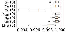
(a) G4

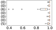
(b) G8

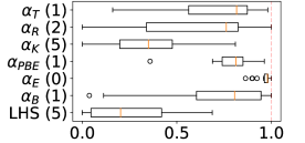
(c) G9

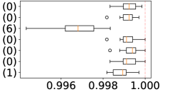
(d) G19

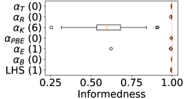
(e) G24

Figure 2: Performance comparison for the selected test problems. The number in brackets show how many alternative acquisition functions beats it statistically significantly in informedness. The state of the art $\alpha_{K}$ is statistically significantly beaten in all problems by the best, and in G4 it is beaten by the naive LHS.

We also illustrate an example classifier output using the proposed acquisition function for G24 in Figure 3.

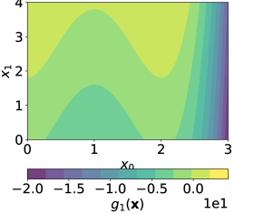
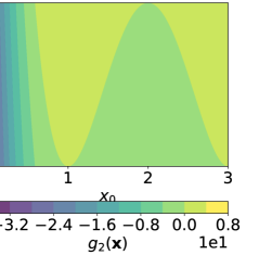
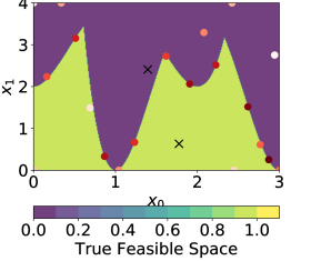
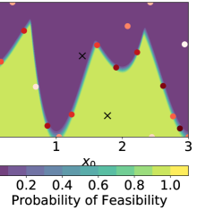
Figure 3: Illustration of the classifier performance in G24. The top row depicts the function landscape for the two constraint functions $g_{1}(\mathbf{x})$ and $g_{2}(\mathbf{x})$. On the bottom row, the black crosses portray the initial samples, and the coloured dots show the samples taken using the proposed acquisition function with darker colour representing later samples. On the bottom left, we show the true feasible space with light green showing the feasible space. On the bottom right, we show the predicted feasible space using our method after only $22$ samples were taken. This clearly shows that the samples taken are often on the boundary, and the final feasibility predictions are good estimations of the true feasible space.

5 Relationship with Constrained Optimisation

Apart from design exploration applications, the ability to accurately determine the feasible space using our method may also be useful in constrained global optimisation of problems. We believe that our work can be complementary to constrained optimisation approaches, since we can construct a classifier of feasibility before performing optimisation. This approach may be useful during the preliminary stages of optimisation when we are trying to understand the problem at hand, and may assist us in determining the true constraints and the character of objective functions.

In Bayesian optimisation for constrained problems, most acquisition functions locate solutions with certain characteristics: those with a high probability of feasibility and those with the greatest expected improvement. For more on this subject, we refer the interested reader to [picheny:sur-opt, li:maxform, bagheri:constraint].

The acquisition functions proposed in this paper do not directly target optimisation. Instead, they seek to locate solutions at the boundary between the feasible and infeasible spaces. In most cases, this will improve the accuracy of the feasibility classification. However, if the acquisition function is driven by the probability of feasibility only, the algorithm is biased to choose solutions away from the boundary. In fact, Knudde et al. [knudde:active] compared against probability of feasibility as a basis of search to improve the classifier. Their results convincingly showed that probability of feasibility understandably performs worse than their proposed method. As such, we refrained from comparing against probability of feasibility in this paper.

In future, we propose to investigate the efficacy of creating an accurate classifier for feasibility prior to optimisation, and evaluating its usefulness in constrained optimisation.