Multithreaded event-chain Monte Carlo with local times

Abstract

We present a multithreaded event-chain Monte Carlo algorithm (ECMC) for hard spheres. Threads synchronize at infrequent breakpoints and otherwise scan for local horizon violations. Using a mapping onto absorbing Markov chains, we rigorously prove the correctness of a sequential-consistency implementation for small test suites. On x86 and ARM processors, a C++ (OpenMP) implementation that uses compare-and-swap primitives for data access achieves considerable speed-up with respect to single-threaded code. The generalized birthday problem suggests that for the number of threads scaling as the square root of the number of spheres, the horizon-violation probability remains small for a fixed simulation time. We provide C++ and Python open-source code that reproduces all our results.

1 Introduction

Event-chain Monte Carlo (ECMC) [1, 2] is an event-driven realization of a continuous-time irreversible Markov chain that has found applications in statistical physics [3, 4] and related fields [5]. Initially restricted to hard spheres and to models with piece-wise constant pair potentials [6], ECMC was subsequently extended to continuous potentials, such as spin models and all-atom particle systems with long-range interactions [7, 8]. Potentials need not be pair-wise additive [9]. In opposition to standard Monte Carlo methods, such as the Metropolis algorithm [10], ECMC does not evaluate the potential $U(\mathbf{x})$ of a configuration $\mathbf{x}$ (nor any ratio of potentials) in order to sample the Boltzmann distribution $\pi(\mathbf{x})=\exp\left[-\beta U(\mathbf{x})\right]$, with inverse temperature $\beta$.

For hard spheres, ECMC is a special case of event-driven molecular dynamics [11, 12]. In molecular dynamics, usually all $N$ spheres have non-zero velocities, and the number of candidate collision events at any time is $\mathcal{O}\left(N\right)$. A central scheduler, efficiently implemented through a heap data structure, yields the next collision with computational effort $\mathcal{O}\left(1\right)$, and it updates the heap in at most $\mathcal{O}\left(\log\!\,N\right)$ operations [13, 14]. Event times are global, and the CPU clock advances together with the collision times. The global collision times and the required communication at each event complicate multithread implementations [15, 16, 17, 18, 19]. Domain decomposition, another strategy to cope with synchronization, is also problematic [20].

In hard-sphere ECMC, a set $\mathcal{A}_{t}$ of $k<N$ “active” spheres (all of radius $\sigma$) have the same non-zero velocity $\mathbf{v}$ that changes infrequently. All other spheres are “static”. At a lifting [21] $l_{t}=([i\!\!\to\!\!j],(\mathbf{x},\mathbf{x}^{\prime}),t)$, an active sphere $i$ collides at time $t$ with a target sphere $j$, at contact $|\mathbf{x}^{\prime}-\mathbf{x}|=2\sigma$ (a condition that must be adapted for periodic boundary conditions). The lifting $l_{t}$ connects an in-state (the configuration just before time $t$, at time $t^{-}$) with an out-state (the configuration just after time $t$, at time $t^{+}$):

$$\text{in-state}:\left[\begin{aligned} i\in\mathcal{A}_{t^{-}},&\quad j\not\in\mathcal{A}_{t^{-}}\\ \mathbf{x}_{i}(t^{-})&=\mathbf{x}\\ \mathbf{x}_{j}(t^{-})&=\mathbf{x}^{\prime}\\ \mathbf{v}_{i}(t^{-})&=\mathbf{v}\\ \mathbf{v}_{j}(t^{-})&=0\\ \end{aligned}\right];\quad\text{out-state}:\left|\begin{aligned} i\not\in\mathcal{A}_{t^{+}},&\quad j\in\mathcal{A}_{t^{+}}\\ \mathbf{x}_{i}(t^{+})&=\mathbf{x}\\ \mathbf{x}_{j}(t^{+})&=\mathbf{x}^{\prime}\\ \mathbf{v}_{i}(t^{+})&=0\\ \mathbf{v}_{j}(t^{+})&=\mathbf{v}\\ \end{aligned}\right|.$$ (1)

We consider in this paper two-dimensional spheres in a square box with periodic boundary conditions. In this system, the direction of $\mathbf{v}$ must be changed at certain breakpoints for the algorithm to be irreducible [22]. However, we restrict our attention to ECMC in between two such breakpoints $h$ and $h^{\prime}$ with, for concreteness, $\mathbf{v}=(v_{x},v_{y})=(1,0)$. For a generic “lifted” [21] initial configuration $\{\mathcal{C}_{h},\mathcal{A}_{h}\}$ at $h$, ECMC is deterministic up to $h^{\prime}$. Generically no two liftings take place at the same time $t$, so that they can be identified by their time.

Our multithreaded ECMC algorithm propagates $k=|\mathcal{A}|$ active spheres in independent threads, with shared memory. In between $h$ and $h^{\prime}$, it only uses local-time attributes of each sphere. At a lifting $l_{t_{i}}=([i\!\!\to\!\!j],(\mathbf{x},\mathbf{x}^{\prime}),t_{i})$, $j$ synchronizes with $i$ (the local time $t_{j}$ is set equal to $t_{i}$). For a sphere $i$ to move, it must not violate certain horizon conditions of nearby spheres $j$. In the absence of horizon violations between $h$ and $h^{\prime}$, multithreaded ECMC will be proven equivalent to the global-time process.

The motivation for our work is twofold. First, we strive to speed up current hard-sphere simulations where, typically, $N\sim 1\!\times\!10^{6}$. These simulations require weeks or month of run time to decorrelate from the initial configuration [3, 23]. Using a connection to the generalized birthday problem in mathematics, we will argue that such simulations can successfully run with $k\lesssim\sqrt{N}$. Our approach to multithreading thus uses the freedom to tune the number of active spheres. Second, by providing proof of concept for multithreaded ECMC algorithms, we hope to motivate the development of parallel ECMC algorithms for other system where sequential ECMC applies already.

The multithreaded ECMC algorithm is presented in two versions. One implementation uses the sequential-consistency model [24]. Mapped onto an absorbing Markov chain, its correctness is rigorously proven for small test suites. The C++ implementation uses OpenMP to map active chains onto hardware threads, together with atomic primitives [25] for fine-grained control of interactions between threads. Considerable speed-up with respect to a single-threaded version is achieved. The few simultaneously moving spheres ($k\ll N$) avoid communication bottlenecks between threads, even though each hard-sphere lifting involves only little computation.

Subtle aspects of our algorithm surface through the confrontation of the C++ implementation with the sequential-consistency computational model on the same test suites. By reordering single statements in the code, we may for example introduce rare bugs that are not detected during random testing, but are readily exhibited in the rigorous solution, and that illustrate difficulties stemming from possible compiler or processor re-ordering.

Code availability.

Cell-based ECMC for two-dimensional hard spheres is implemented (in Fortran90) as CellECMC.f90. Our version is slightly modified from the original code written by E. P. Bernard (see Acknowledgements). The code prepares initial configurations, and it is used in validation scripts.

2 Algorithms: from global-time processes to multithreaded ECMC

In this section, we start with the definition of a continuous-time process, Algorithm 1, that is manifestly equivalent to molecular dynamics with the collision rules of eq. (1). Its event-driven version, Algorithm 1, provides the reference set $\mathcal{L}^{\text{ref}}$of liftings used in our validation scripts (see Section 3). The single-threaded Algorithm 3 relies on local times. It has correct output if no horizon violation takes place. Its event-driven version, Algorithm 2, yields a practical method that can be implemented and tested. Algorithms 5 and 6 realize multithreaded ECMC, the latter in a highly efficient C++ implementation.

2.1 Continuous processes and ECMC with global time

Algorithm 1 (Continuous process with global time).

At global time $t=h$, an initial lifted configuration $\{\mathcal{C}_{h},\mathcal{A}_{h}\}$ is given ($\mathbf{v}_{i}=\mathbf{v}=(1,0)\ \forall i\in\mathcal{A}_{h}$ and $\mathbf{v}_{i}=0\ \forall i\not\in\mathcal{A}_{h}$). All spheres $i$ carry local times $t_{i}$, with, initially, $t_{i}(h)=h\ \forall i$. For active spheres ($i\in\mathcal{A}_{t}$), $\mathrm{d}t_{i}/\mathrm{d}t=1$. At a lifting $l_{t}=([i\!\!\to\!\!j],(\mathbf{x},\mathbf{x}^{\prime}),t)$ the local time of sphere $j$ is updated as $t_{j}(t^{+})=t$ and, furthermore, $\mathcal{A}_{t^{+}}=\mathcal{A}_{t^{-}}\setminus\{i\}\cup\{j\}$. The algorithm stops at global time $t=h^{\prime}$, and outputs the lifted configuration $\{\mathcal{C}_{h^{\prime}},\mathcal{A}_{h^{\prime}}\}$, and the set $\mathcal{L}_{h^{\prime}}=\{l_{t}:h<t<h^{\prime}\}$ of liftings that have taken place between $h$ and $h^{\prime}$.

Remark 1 (Meaning of local times).

In Alg. 1, the local time $t_{i}(t)$ is a function of the global time $t$. It gives the global time at which sphere $i$ was last active (or $t_{i}(t)=h$ if $i$ was not active for $[h,t]$). Therefore $t_{i}(t)=t\ \forall i\in\mathcal{A}_{t}$ and $t_{i}(t)<t\ \forall i\not\in\mathcal{A}_{t}$.

Remark 2 (Positivity of local-time updates).

In Alg. 1, at any lifting $l_{t}$, the update of $t_{j}$ is positive: $t_{j}(t^{+})-t_{j}(t^{-})>0$.

Remark 3 (Time-reversal invariance).

Alg. 1 is deterministic and time-reversal invariant: If an initial lifted configuration $\{\mathcal{C}_{h},\mathcal{A}_{h}\}$ generates the final lifted configuration $\{\mathcal{C}_{h^{\prime}},\mathcal{A}_{h^{\prime}}\}$ with $\mathbf{v}$, then the latter will reproduce the initial configuration with $-\mathbf{v}$. The set $\mathcal{L}$ of liftings is the same in both cases.

In order to converge towards a given probability distribution, Markov-chain algorithms must satisfy the global-balance condition. It states that the probability flow into a configuration $\mathcal{C}$ (summed over all liftings $\mathcal{A}$) must equal the probability flow out of it [22]. ECMC balances these flows for each lifting individually (for the uniform probability distribution).

Lemma 1.

Alg. 1 satisfies the global-balance condition for any lifted configuration $\{\mathcal{C},\mathcal{A}\}$. All lifted configurations accessible from a given initial configuration thus have the same statistical weight.

Proof.

The algorithm is equivalent to molecular dynamics that conserves one-dimensional momenta as well as the energy. The claimed property follows for Alg. 1 because it is satisfied by molecular dynamics. The property can be shown directly for a discretized version of Alg. 1 on a rectangular grid aligned with $\mathbf{v}$ with infinitesimal cell size such that each lifted configuration $\{\mathcal{C},\mathcal{A}\}$ has a unique predecessor. The flow into each lifted configuration equals one. This is equivalent to global balance for the uniform probability distribution. ∎

The event-driven version of Algorithm 1 is the following:

Algorithm 2 (ECMC with global time).

With input as in Alg. 1, in each iteration $I=1,2,\dots$, the next global lifting time is computed as $t_{I+1}=t_{I}+\min_{i\in\mathcal{A},j\not\in\mathcal{A}}\tau_{ij}$, where $\tau_{ij}$ is the time of flight from sphere $i$ to sphere $j$. At time $t_{I}$, local times and positions of active spheres are advanced to $\tilde{t}=\min\left(t_{I+1},h^{\prime}\right)$, and to $\mathbf{x}_{i}(t_{I+1})=\mathbf{x}_{i}(t_{I})+(\tilde{t}-t_{I})\mathbf{v}$, respectively. If $\tilde{t}=t_{I+1}$ (a lifting $l_{I+1}=(\{i,j\},\{\mathbf{x},\mathbf{x}^{\prime}\},t_{I+1})$ takes place), the set of active spheres is updated as $\mathcal{A}_{I+1}=\mathcal{A}_{I}\setminus\{i\}\cup\{j\}$. Otherwise $\tilde{t}=h^{\prime}$, and the algorithm stops. Output is as in Alg. 1.

Code availability.

Alg. 1 is implemented in GlobalTimeECMC.py and invoked in several validation scripts, for which it generates the reference lifting sets $\mathcal{L}^{\text{ref}}$.

2.2 Single-threaded processes and ECMC with local times

Algorithm 3, that we now describe, is a single-threaded emulation of our multithreaded Algorithms 5 and 6. A randomly sampled active chain $\iota\in\{1,2,\dots\}$ advances (in what corresponds to a thread) for an imposed duration, at most until its local time reaches $h^{\prime}$. On thread $\iota$, the active sphere $i$ must remain above the horizons of its neighboring spheres $j$ (see Fig. 1a). The horizon condition is

$$t_{i}+\tau_{ij}>t_{j},$$ (2)

where the time of flight is $\tau_{ij}=x_{j}-x_{i}+b_{ij}$, with $b_{ij}$ the contact separation parallel to $\mathbf{v}$ between spheres $i$ and $j$. The horizon condition must be checked for at most three spheres $j$ for a given $i$ because all other spheres are either too far for lifting with $i$ in the direction perpendicular to $\mathbf{v}$ or are prevented from lifting with $i$ by other spheres (see Section 3.1). The algorithm aborts if a horizon violation is encountered. The active chain $\iota$ stops if a lifting would be to a sphere $j$ that is itself active. The active chain $\iota+1$ is then started.

Remark 4 (Double role of horizon condition).

The horizon condition of eq. (2) has two roles. First, it is a necessary condition for a lifting of $i$ with $j$ (if it effectively takes place) to produce the required positive local-time update of $t_{j}$ at the lifting time $t$ (see Remark 2 and Fig. 1a). Second, it is a sufficient non-crossing condition for any sphere $k$, ensuring that $k$ was not at a previous local time in conflict with $i$ (see Fig. 1b).

It is for the second role discussed in Remark 4 that the horizon condition is checked for all neighboring spheres $j$ of an active sphere $i$.

Remark 5 (False alarms from horizon condition).

The horizon condition may lead to false alarms (see Fig. 1b), which could be avoided through the use of the non-crossing condition. The latter is more difficult to check, as it requires the history of past liftings. Our algorithms only implement the horizon condition.

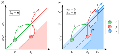
Figure 1: Horizon condition and non-crossing condition in local-time algorithms. (a): Sphere $i$ is above the horizon of sphere $j$ (shaded area), so that at the lifting of $i$ with $j$, the local-time update of $t_{j}$ is positive. (b): Sphere $i$ does not lift with $k$. It does not cross the past trajectory of $k$, although it violates the horizon condition with $k$ (light shading) (supposing $b_{ik}=0$). The lifting of $i$ with $j$ could in principle be allowed under the non-crossing condition with $k$ (dark blue shading), supposing $\tau_{jk}=\infty$.

Algorithm 3 (Single-threaded continuous process with local times).

With input as in Alg. 1, active chain $\iota=1,2,\dots$ is initialized (sequentially) with an active sphere $i$, sampled from $\tilde{\mathcal{A}}=\{i\in\mathcal{A},t_{i}\neq h^{\prime}\}$, and for a local-time interval $\tau^{\max}_{\iota}=\min\left(\operatorname{ran},h^{\prime}-t_{i}\right)$, where $\operatorname{ran}$ is a positive random number. In active chain $\iota$, the active sphere $i$ moves with velocity $\mathbf{v}$ for $\tau\in[0,\tau^{\max}_{\iota}]$ and $\mathrm{d}t_{i}/\mathrm{d}\tau=1$, if the horizon condition of eq. (2) is satisfied for all spheres $j$. (In case of a horizon violation, the algorithm aborts.) If a lifting $l_{t_{i}}=([i\!\!\to\!\!j],(\mathbf{x},\mathbf{x}^{\prime}),t_{i})$ concerns an active sphere $j$, the active chain $\iota$ stops with $i$ at $\mathbf{x}$. Otherwise, the local time of sphere $j$ is updated as $t_{j}(t_{i}^{+})=t_{i}$ and $\mathcal{A}=\mathcal{A}\setminus\{i\}\cup\{j\}$, with the active chain $\iota$ now moving $j$. The algorithm terminates if $\tilde{\mathcal{A}}=\emptyset$, that is, if all the active spheres are stalled. Output is as for Alg. 1.

Remark 6 (Stalled spheres).

“Stalled” spheres (active spheres $i$ with $t_{i}=h^{\prime}$) make up the set $\mathcal{A}\setminus\tilde{\mathcal{A}}$. Considering stalled spheres separately simplifies the sampling of $\tilde{\mathcal{A}}$, and the restart from $h^{\prime}$ for the next leg of the ECMC run.

Lemma 2.

If Alg. 3 terminates without a horizon violation, its output is identical to that of Alg. 1.

Proof.

We consider the final lifted configuration $\{\mathcal{C}_{h^{\prime}},\mathcal{A}_{h^{\prime}}\}$ of a run that has terminated without a horizon violation, and that has preserved a log of all local-time updates. The termination condition is $\tilde{\mathcal{A}}=\emptyset$, so that all active spheres are stalled, with local time $h^{\prime}$. We further consider the final lifting $l_{h^{\prime\prime}}$ in $\mathcal{L}_{h^{\prime}}$ (so that $t<h^{\prime\prime}\ \forall\ l_{t}\in\mathcal{L}_{h^{\prime\prime}}$). Local times of static spheres satisfy $t_{i}\leq h^{\prime\prime}\ \forall i\not\in\mathcal{A}_{h^{\prime}}$. When backtracking, using Alg. 1 with $-\mathbf{v}$, from $h^{\prime}$ to $h^{\prime\prime+}$, no lifting takes place among active spheres (see Fig. 2a). The area swept out by the active spheres cannot overlap with a static sphere $j$ because it must have $t_{j}<h^{\prime\prime}$ (local times are smaller than the last lifting) and, on the other hand, $t_{j}>h^{\prime\prime}$, because of eq. (2) (see Fig. 2b). The lifting $l_{h^{\prime\prime}}=([i\!\!\to\!\!j],(\mathbf{x},\mathbf{x}^{\prime}),h^{\prime\prime})$ can now be undone. (From $j\in\mathcal{A}_{h^{\prime}}$ and $i\not\in\mathcal{A}_{h^{\prime}}$, we obtain $\mathcal{A}_{h^{\prime\prime}}=\mathcal{A}_{h^{\prime}}\setminus\{j\}\cup\{i\}$. The updated local time $t_{j}(h^{\prime\prime-})$ can be reconstructed from the log. It is smaller than $h^{\prime\prime}$. The lifting is then itself eliminated: $\mathcal{L}_{h^{\prime\prime}}=\mathcal{L}_{h^{\prime}}\setminus\{l_{h^{\prime\prime}}\}$.) All active spheres at $h^{\prime\prime-}$ now have local time $h^{\prime\prime}$. Similary, all liftings can be undone, effectively running Alg. 1 with $-\mathbf{v}$ from $h^{\prime}$ to $h$. As Alg. 1 is time-inversion invariant, the local times at its liftings are the same as those of Alg. 3. ∎

Figure 2: Backtrack using Alg. 1 from the final configuration of Alg. 3. (a): Active spheres $k$ and $l$ do not lift among each other. (b): A static sphere $j$ crossing the trajectory of active sphere $k$. This crossing is impossible because of the horizon condition ($\tilde{\tau}<h^{\prime}-h^{\prime\prime}$ leading to $t_{j}>h^{\prime\prime}$, in contradiction with the condition $t_{j}<h^{\prime\prime}$).

For concreteness, in the following event-driven formulation of Algorithm 3, the local-time interval $\tau_{\iota}^{\max}$ of an active chain $\iota$ is chosen equal to the time of flight towards the next lifting.

Algorithm 4 (Single-threaded ECMC with local times).

With input as in Alg. 1, for each (sequential) active chain $\iota=1,2,\dots$, an active sphere $i$ is sampled from $\tilde{\mathcal{A}}=\{i\in\mathcal{A},t_{i}\neq h^{\prime}\}$. The horizon conditions of eq. (2) are checked for all spheres $j$ that can have finite time of flight $\tau_{ij}$. The algorithm aborts if a violation occurs. Otherwise, $i$ is moved forward to $\min\left(t_{i}+\tau_{ij},h^{\prime}\right)$, and the local time of $i$ and $j$ are updated to that time. The active chain stops if $j$ is an active sphere or if the local time equals $h^{\prime}$. Otherwise, the move corresponds to a lifting $l_{t_{i}+\tau_{ij}}=([i\!\!\to\!\!j],(\mathbf{x},\mathbf{x}^{\prime}),t_{i}+\tau_{ij})$ and $\mathcal{A}=\mathcal{A}\setminus\{i\}\cup\{j\}$, with the active chain now moving $j$. The algorithm terminates if $\tilde{\mathcal{A}}=\emptyset$. Output is as for Alg. 1.

Code availability.

Alg. 2 is implemented in SingleThreadLocalTimeECMC.py and tested in the PValidateECMC.sh script.

Remark 7 (Partial validation).

In Section 3.2, a variant of Alg. 2 is used to validate part of a run, even if it does not terminate correctly. When a sphere $i$ detects a horizon violation, its time $t_{i}$ is recorded. At $h^{\prime}$, the set $\mathcal{L}_{t^{*}}$ of all liftings up to the earliest horizon violation, at $t^{*}$, agrees with the corresponding partial list of liftings for Alg. 1.

2.3 Multithreaded ECMC (sequential-consistency model)

Algorithm 5, the subject of the present section, is a model shared-memory ECMC on $k$ threads, that is, on as many threads as there are active spheres. The algorithm adopts the sequential-consistency model [24]. We rigorously prove its correctness for small test suites by mapping the multithreading stage of this algorithm to an absorbing Markov chain. The algorithm allows us to show that certain seemingly innocuous modifications of Algorithm 6 (the C++ implementation) contain bugs that are too rare to be detected by routine testing.

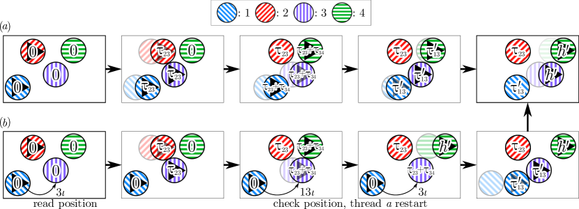
Figure 3: Alg. 5, as applied to the SequentialC4 test suite. (a): Reference set $\mathcal{L}^{\text{ref}}$from Alg. 1. (b): Run of Alg. 5 involving a “lock-less” lock rejection on the position of sphere $3$.

The algorithm has three stages. In the (sequential) initialization stage, it inputs a lifted initial configuration and maps each active sphere to a thread. This is followed by the multithreading stage, where each active chain progresses independently, checking the horizon conditions in its local environment. The algorithm concludes with the (sequential) output stage.

At each step of the multithreading stage of Algorithm 5, a switch randomly selects one of the $k$ statements (one for each thread $a,b,\dots$) contained in a buffer as $\{\text{next}_{a},\text{next}_{b},\dots\}$. The selected statement is executed on the corresponding thread, and then the buffer is updated. The random sequence of statements mimics the absence of thread synchronization except at breakpoints. All threads possess an absorbing wait statement. When it is reached throughout, the algorithm progresses to the output stage, followed by successful termination. The program aborts when a thread detects a horizon violation. For our test suites, we prove by explicit construction that each state is connected to at least one of the absorbing states, but we lack a general proof of validity for arbitrary configurations and general $N$.

In Algorithm 5, each sphere has three attributes, namely a tag, a local time and a position. The sphere’s tag indicates whether it is active on a thread $\iota$, stalled, or static. All threads have read/write access to the attributes of all spheres. A state of the Markov chain is constituted by the spheres with their attributes, some local variables and the buffer content.

Algorithm 5 (Multithreaded ECMC (sequential-consistency model)).

At breakpoint $h=0$, a lifted initial configuration $\{\mathcal{C}_{h},\mathcal{A}_{h}\}$ is input (see Fig. 3 for the example with four spheres). All local times are set to $h=0$, all tags are put to static, except for the active spheres, whose tags correspond to their thread $\iota$. The buffer is set to $\{1_{1},\ 1_{\iota},\ldots,1_{k}\}$. A random switch selects one buffer element. The corresponding statement is executed on its thread, and the buffer is replenished. The following provides pseudo-code for the multithreading stage ($i_{\iota}$ is the active sphere, $j_{\iota}$ the target sphere, and $distance_{\iota}$ the difference between $h^{\prime}$ and the local time, all on thread $\iota$.):

$1\iota$	$\tau_{\iota}\leftarrow\text{distance}_{\iota}$; $j_{\iota}\leftarrow i_{\iota}$; $x_{\iota}\leftarrow\infty$
$2\iota$	for j̃ in ${\text{\{}1,2,...,n\}}\setminus i_{\iota}$ :
$3\iota$	$x_{\text{\~{\j}}}\leftarrow{\text{\~{\j}}}.x$
$4\iota$	$\tau_{i{\text{\~{\j}}}}\leftarrow x_{\text{\~{\j}}}-i_{\iota}.x-b_{i{\text{\~{\j}}}}$
$5\iota$	if $i_{\iota}.t\!+\!\tau_{i{\text{\~{\j}}}}\!<\!{\text{\~{\j}}}.t$ : abort
$6\iota$	if $\tau_{i{\text{\~{\j}}}}<\tau_{\iota}$ :
$7\iota$	$j_{\iota}\leftarrow{\text{\~{\j}}}$
$8\iota$	$x_{\iota}\leftarrow x_{{\text{\~{\j}}}}$
$9\iota$	$\tau_{\iota}\leftarrow\tau_{i{\text{\~{\j}}}}$
$10\iota$	$j_{\iota}.tag.$CAS$(static,\iota)$
$11\iota$	if $j_{\iota}.tag=\iota$ :
$12\iota$	if $\tau_{\iota}<\text{distance}_{\iota}$ :
$13\iota$	if $x_{\iota}=j_{\iota}.x$ :
$14\iota$	$j_{\iota}.t\leftarrow i_{\iota}.t+\tau_{\iota}$
$15\iota$	$i_{\iota}.t\leftarrow i_{\iota}.t+\tau_{\iota}$
$16\iota$	$i_{\iota}.x\leftarrow i_{\iota}.x+\tau_{\iota}$
$17\iota$	$i_{\iota}.tag\leftarrow static$
$18\iota$	$\text{distance}_{\iota}\leftarrow\text{distance}_{\iota}-\tau_{\iota}$
$19\iota$	$i_{\iota}\leftarrow j_{\iota}$
	else :
$20\iota$	$j_{\iota}.tag\leftarrow static$
	goto $1$
	else :
$21\iota$	$i_{\iota}.t\leftarrow i_{\iota}.t+\tau_{\iota}$
$22\iota$	$i_{\iota}.x\leftarrow i_{\iota}.x+\tau_{\iota}$
$23\iota$	$\text{distance}_{\iota}\leftarrow 0$
$24\iota$	$i_{\iota}.tag\leftarrow stalled$
	else : goto $1$
$25\iota$	if $\text{distance}_{\iota}>0$ : goto $1$
$26\iota$	wait

When all $k$ threads have reached their wait statements, the algorithm proceeds to its output stage. Output is as for Alg. 1.

Code availability.

SequentialMultiThreadECMC.py. implements Alg. 5. It also constructs all states connected to the initial state and traces them to the absorbing states.

Remark 8 (Illustration of pseudocode).

The multithreading stage of Alg. 5 corresponds in $k$ independent programs running independently. In the sequential-consistency model, the space of programming statements is thus $k$-dimensional (one sequence $(1\iota,\ldots,26\iota)$ per thread), and each displacement in this space proceeds along a randomly chosen coordinate axis. As an example, if for a buffer $\{next_{1},\ldots,next_{\iota}=20\iota,\ldots,next_{k}\}$ the switch selects thread $\iota$, then the tag of target particle $j_{\iota}$ is set to “static”, and the buffer is updated to $\{next_{1},\ldots,next_{\iota}=1\iota,\ldots,next_{k}\}$. The thread $\iota$ will thus be restarted at its next selection.

The compare-and-swap (CAS) statement in $10\iota$ of Algorithm 5 amounts to a single-line if. It is equivalent to: “if $j_{\iota}.tag=static$  : $j_{\iota}.tag=\iota$” (if $j$ is static, then it is set to active on thread $\iota$ (see Remark 3 for a discussion).

We prove correctness of Algorithm 5, for the SequentialC4 test suite with $N=$ and $k=2$ (see Fig. 3), that we later extend to the SequentialC5 test suite with $N=5$.

Lemma 3.

If Alg. 5 terminates without a horizon violation, its output (for the SequentialC4 test suite) is identical to that of Alg. 1.

Proof.

In the SequentialC4 test suite with threads “$a$” and “$b$” we suppose that the switch samples $a$ and $b$ with equal probabilities. The two-thread stage of Alg. 5 then consists in a finite Markov chain with the $3670$ states $S_{n}$ that are accessible from the initial state. The abort state has no buffer content. All other $3669$ states comprise the buffer $\{\text{next}_{a},\text{next}_{b}\}$, the sphere objects (the spheres and their attributes: tag, local time, position), and some thread-specific local variables. One iteration of the Markov chain (selection of $\text{next}_{a}$ or $\text{next}_{b}$, execution of the corresponding statement, buffer update) realizes the transition from $S_{n}$ to a state $S_{m}$ with probability $T_{nm}=1/2$. The $3670\times 3670$ transition matrix $T=(T_{nm})$ has unit diagonal elements for the abort, and for the unique terminate state with buffer $\{26a,26b\}$, which are both absorbing states of the Markov chain. Furthermore, we can show explicitly that all $3670$ states have a finite probability to reach an absorbing state in a finite number of steps. This proves that the Markov chain is absorbing. For an absorbing Markov chain, all states that are not absorbing are transient, and they die out at large times. The algorithm thus either ends up in the unique terminate state that corresponds to successful completion, or else in the abort state. ∎

All states of the Markov chain may be projected onto their buffer $\{\text{next}_{a},\text{next}_{b}\}$ and visualized (see Fig. 4)).

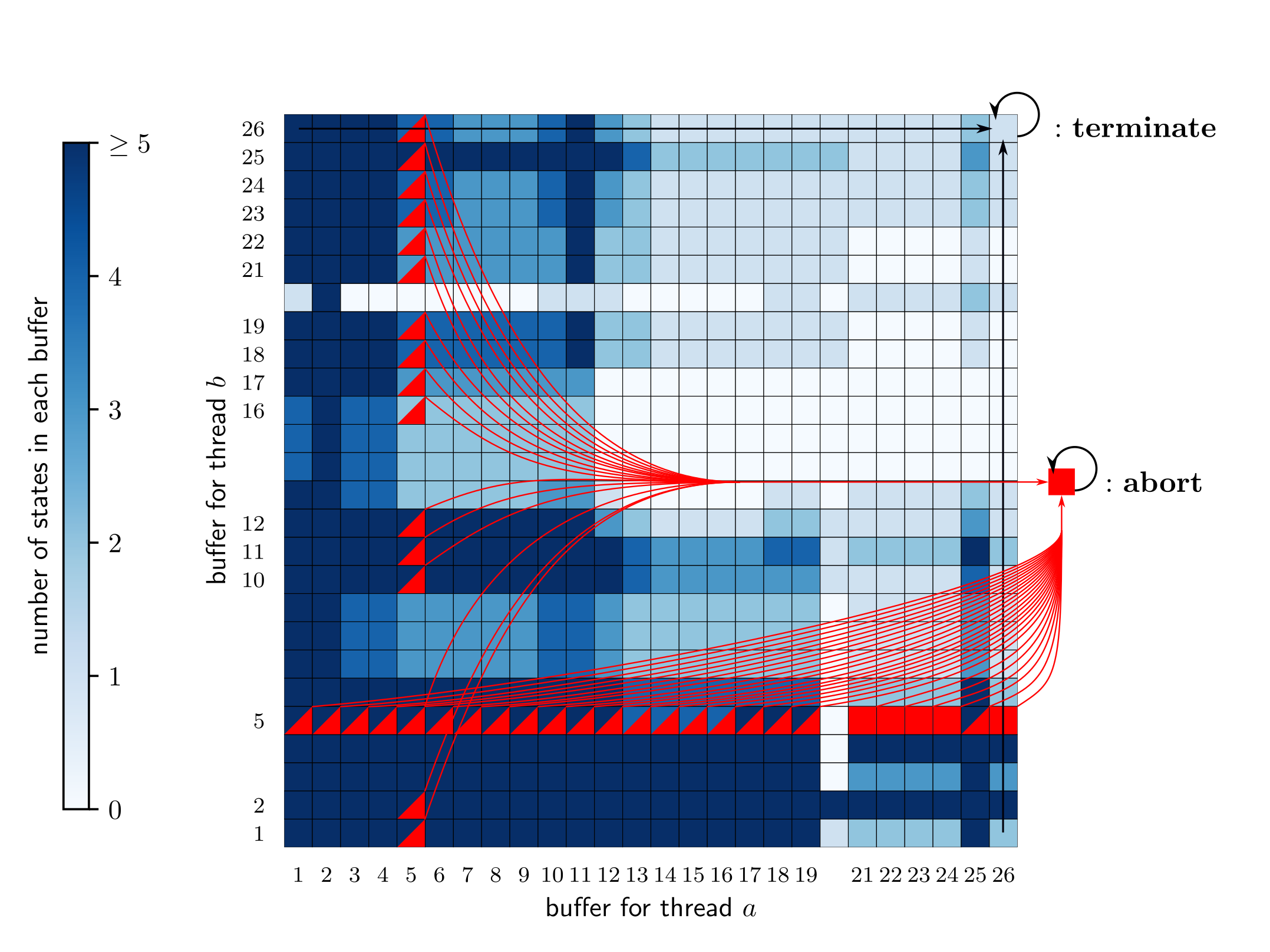
Figure 4: The $3670$ states in Alg. 5 for the SequentialC4 test suite projected onto the buffer content $\{\text{next}_{a},\text{next}_{b}\}$ (see Fig. 3). The terminate buffer $\{26a,26b\}$ corresponds to a single state.

Remark 9 (CAS statement).

The CAS statements (see $10\iota$ in Alg. 5) acquire their full meaning in the multithreaded Alg. 6 The way in which they differ from simple if statements can already be illustrated in the simplified setting. We suppose two threads $a$ and $b$. Then, with $j_{\iota}$ the target sphere on thread $\iota$, a buffer content $\{10a,10b\}$:
⋮ ⋮ $10a$ $j_{a}.tag.$CAS($static,a$) $11a$ if $j_{a}.tag=a$ : ⋮ ⋮ ⋮ ⋮ $10b$ $j_{b}.tag.$CAS$(static,b)$ $11b$ if $j_{b}.tag=b$ : ⋮ ⋮ can belong to a state with $j_{a}=3=j_{b}=3$.. If the statement $10a$ is selected, sphere $3$ becomes active on thread $a$ (through the statement $3.tag=a$). In contrast, if the switch selects $10b$, sphere $3$ becomes active on thread $b$. The program continues consistently for both switch choices, because the selection is made in a single (“atomic”) step on each thread and because the sequential-consistency model avoids conflicting memory assignments. In contrast, if the switch selection from $\{10a,10b\}$ is split as:
⋮ ⋮ $10^{\prime}a$ if $j_{a}.tag=static$ : $10^{\prime\prime}a$ $j_{a}.tag=a$ $11a$ if $j_{a}.tag=a$ : ⋮ ⋮ ⋮ ⋮ $10^{\prime}b$ if $j_{b}.tag=static$ : $10^{\prime\prime}b$ $j_{b}.tag=b$ $11b$ if $j_{b}.tag=b$ : ⋮ ⋮ the sequence $10^{\prime}a\to 10^{\prime}b\to 10^{\prime\prime}a\to 11a\to 10^{\prime\prime}b\to 11b$ results in sphere $3$ first becoming active on thread $a$ (and the thread continuing as if this remained the case), and then on thread $b$, which is inconsistent. In Algorithm 6, the C++ implementation of multithreaded ECMC, the CAS likewise keeps this selection step atomic, and likewise excludes memory conflicts among all threads during this step. It thus plays the role of a lightweight memory lock.

Algorithm 5 features lock-free programming, which is also a key ingredient of Algorithm 6.

Remark 10 (Lock-free programming).

To illustrate lock-free programming in Alg. 5, we consider two threads, $a$ and $b$.
$7a$         $j_{a}\leftarrow{\text{\~{\j}}}$ $8a$         $x_{a}\leftarrow x_{{\text{\~{\j}}}}$ ⋮ ⋮ $10a$ $j_{a}.tag.$CAS$(static,a)$ ⋮ ⋮ $13a$         if $x_{a}=j_{a}.x$ : ⋮ ⋮ ⋮ ⋮ $16b$           $i_{b}.x\leftarrow i_{b}.x+\tau_{b}$ $17b$           $i_{b}.tag\leftarrow static$ ⋮ ⋮ The identification of the target sphere $j_{a}$ on thread $a$ (statements $7a$ and $8a$) would be compromised if, before locking through the CAS statement at $10a$, it was changed in thread $b$, where the same sphere $i_{b}$ is active (see statements $16b,17b$). However, the statement $13a$ checks that sphere $j_{a}$ has not moved. If this condition is not satisfied, the thread $a$ will end up being restarted (through statement $20a$). (See also Remark 12.)

2.4 Multithreaded ECMC (C++, OpenMP implementation)

Algorithm 6, discussed in this section, translates Algorithm 5 into C++ (OpenMP). The CAS statement and lock-free programming assure its efficiency. A sphere’s attributes are again its position, its local time, and its tag. The latter is a an atomic variable. We refer to line numbers in Algorithm 5.

Algorithm 6 (Multithreaded ECMC (C++, OpenMP)).

With initial values as in Alg. 1, thread management is handled by OpenMP. The number of threads can be smaller than the number of active spheres. The multithreading stage transliterates the one of Alg. 5. Statement $2\iota$ of Alg. 5 is implemented through a constraint graph (see Section 3.1). Statements $10\iota$ through $13\iota$ are expressed as follows in MultiThreadECMC.cc:
$10\iota$ $\rightarrow$ j->tag.compare_exchange_strong(...static,... $11\iota$ $\rightarrow$ if (j->tag.load(memory_order) == iota) $12\iota$ $\rightarrow$ if (tau < distance) $13\iota$ $\rightarrow$ if (x == j->x),
where the memory_order qualifier may take on different values (see Section 3.2). Important differences with Alg. 5 are discussed in Remarks 11 and 12. Output is as for Alg. 1.

Code availability.

Alg. 6 is implemented in MultiThreadECMC.cc. It is executed in several validation and benchmarking scripts (see Section 3.2).

Remark 11 (Active-sphere necklaces).

Alg. 5 restarts thread $\iota$ if the target sphere $j$ (for an active sphere $i$ on the thread) is itself active on another thread. With periodic boundary conditions, active-sphere necklaces, where all target spheres are active, can deadlock the algorithm. To avoid this, Alg. 6 moves sphere $i$ up to contact with $j$ before restarting (this is also used in Alg. 2).

The source code of Algorithm 6 essentially translates that of Algorithm 5. The compiler may however change the order of execution for some statements in order to gain efficiency. (The memory access in modern multi-core processors can also be very complex and, in particular, thread-dependent.) Attributes, such as the memory_order qualifier in the CAS statement, may constrain the allowed changes of order. The reordering directives adopted in Algorithm 6 were chosen and validated with the help of extensive runs from randomly generated configurations. However, subtle pitfalls escaping notice through such testing can be exposed by explicitly reordering statements in Algorithm 5.

Remark 12 (Memory-order directives in Algs 5 and 6).

In the SequentialC5 test suite with $N=5$, interchanging statements $15\iota$ and $16\iota$ in Alg. 5 yields a spurious absorbing state, and invalidates the algorithm. The same test suite can also be input into Alg. 6, where it passes the Ordering.sh validation test, even if the statements in MultiCPP.cc corresponding to $15\iota$ and $16\iota$ are exchanged. However, a $1\mu$s pause statement introduced in the C++ program between what corresponds to the (interchanged) statements $15\iota$ and $16\iota$ produces a $sim1\%$ error rate, illustrating that Alg. 6 is unsafe without a protection of the order of the said statements. Safety may be increased through atomic position and local time variables, allowing the use of the fetch_add() operation to displace spheres.

3 Tools, validation protocols, benchmarks, and extensions

We now discuss the implementations of the algorithms of Section 2, as well as their validation protocols, benchmarks, and possible extensions. We also discuss the prospects of this method beyond this paper’s focus on the interval between two breakpoints $h$ and $h^{\prime}$.

In our implementation of Algorithms 1, 2, and 6, a directed constraint graph encodes the possible pairs of active and target spheres as arrows $[i\!\!\to\!\!j]$ (see Section 3.1). The outdegree of this graph is at most three, and a rough constraint graph $\mathcal{G}^{(3)}$ with, usually, outdegree three for all vertices is easily generated. $\mathcal{G}^{(3)}$ may contain redundant arrows that cannot correspond to liftings. Our pruning algorithm eliminates many of them. We also prove that $\mathcal{G}^{\min}$, the minimal constraint graph, is planar. This may be of importance if disjoint parts of the constraint graph are stored on different CPUs, each with a number of dedicated threads. In general, we expect constraint graphs to be a useful tool for hard-sphere production codes, with typically $\mathcal{O}\left(N\right)$ liftings between changes of $\mathbf{v}$.

Validation scripts are discussed in Section 3.2. Scripts check that the liftings of standard cell-based ECMC are all accounted for in the used constraint graph. For the ECMC algorithms of Section 2, the set $\mathcal{L}$ of liftings provides the complete history of each run, and scripts check that they corresponds to $\mathcal{L}^{\text{ref}}$.

In Section 3.3, we then benchmark Algorithm 6 and demonstrate a speed-up by an order of magnitude for a single CPU with 40 threads on an x86 CPU (see Section 3.3). The overhead introduced by multithreading ($\sim 2.4$) is very reasonable. We then discuss possible extension of our methods (see Section 3.4).

3.1 Constraint graphs

For a given initial condition $\mathcal{C}_{h}$ and velocity $\mathbf{v}$, arrows $[i\!\!\to\!\!j]$ of the constraint graph $\mathcal{G}_{\mathbf{v}}$ represent possible liftings $l_{t}=([i\!\!\to\!\!j],(\mathbf{x},\mathbf{x}^{\prime}),t)$ [26]. Arrows remain unchanged between breakpoints because spheres $i$ and $j$ with a perpendicular distance of less than $2\sigma$ cannot hop over one another (this argument can be adapted to periodic boundary conditions), and pairs with larger perpendicular distance are absent from $\mathcal{G}$. All constraint graphs $\mathcal{G}_{\mathbf{v}}$ are supersets of a minimal constraint graph $\mathcal{G}^{\min}_{\mathbf{v}}\equiv\mathcal{G}^{\min}_{-\mathbf{v}}$ (where the equivalence is understood as $[i\!\!\to\!\!j]_{\mathbf{v}}\equiv[j\!\!\to\!\!i]_{-\mathbf{v}}$).

Remark 13 (Constraint graphs and convex polytopes).

Each arrow $[i\!\!\to\!\!j]$ of the constraint graph $\mathcal{G}_{\mathbf{v}}$ provides (for $\mathbf{v}=(1,0)$) an inequality

$$x_{i} \leq x_{j}-b_{ij}$$ (3)

that is tight ($x_{i}=x_{j}-b_{ij}$) when $i$ lifts to $j$ at contact (if there are configurations $\mathcal{C}$ where it is tight, then $[i\!\!\to\!\!j]$ belongs to $\mathcal{G}^{\min}_{\mathbf{v}}$). The set of inequalities defines a convex polytope. With periodic boundary conditions (unaccounted for in eq. (3)), this polytope is infinite in the direction corresponding to uniform translation of all spheres with $\mathbf{v}$ (see [26]).

Remark 14 (Constraint graphs and irreducibility).

Rigorously, we define the constraint graph $\mathcal{G}^{\min}_{\mathbf{v}}$ as the set of arrows $[i\!\!\to\!\!j]$ that are encountered from $\mathcal{C}_{h}$ by Alg. 1 (or, equivalently, Alg. 1) at liftings $l_{t}\ \forall t\in(-\infty,\infty)$. The liftings for $t<0$ can be constructed because of time-reversal invariance (see Remark 3). For the same reason, we have $\mathcal{G}^{\min}_{\mathbf{v}}\equiv\mathcal{G}^{\min}_{-\mathbf{v}}$, and the set of arrows reached from $\mathcal{C}_{h}$ is equivalent to that reached from any configuration that is reached from $\mathcal{C}$ (and in particular $\mathcal{C}_{h^{\prime}}$). While we expect ECMC to be irreducible in the polytope defined through the inequalities in eq. (3), we do not require irreducibility for the definition of $\mathcal{G}^{\min}$.

Between breakpoints, the active sphere $i$ can lift to at most three other spheres, namely the sphere $j^{0}$ minimizing the time of flight $\tau_{ij}$ in a corridor of width $2\sigma$ around the center of $i$ , and likewise the closest-by sphere $j^{+}$ in the corridors $[\sigma,2\sigma]$ and sphere $j^{-}$ in the corridor $[-2\sigma,-\sigma]$ (see Fig. 5a). The set of arrows $\{[i\!\!\to\!\!j^{0}],[i\!\!\to\!\!j^{-}],[i\!\!\to\!\!j^{+}]\ \forall i\in\{1,\ldots,N\}\}$ constitutes the constraint graph $\mathcal{G}^{(3)}_{\mathbf{v}}$, which is thus easily computed. Except for small systems (when the corridors may be empty) $\mathcal{G}^{(3)}$ has outdegree three for all spheres $i$. However, its indegree is not fixed. The constraint graph $\mathcal{G}^{(3)}$ is not necessarily locally planar, and in the embedding provided by the sphere centers of a given configuration, non-local arrows can be present (see Fig. 6a). However, $\mathcal{G}^{\min}$ can be proven to be locally planar (see Fig. 6b)).

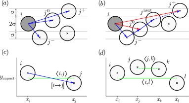
Figure 5: Constraint graphs, pruning, and planarity. (a): Corridors of an active sphere $i$, with arrows $[i\!\!\to\!\!j^{-}]$, $[i\!\!\to\!\!j^{0}]$, and $[i\!\!\to\!\!j^{+}]$ belonging to $\mathcal{G}^{(3)}_{(1,0)}$. (b): Pruning of an arrow $[i\!\!\to\!\!j^{+}]$ through a sphere $j^{\text{next}}$ without there being an arrow $[i\!\!\to\!\!j^{\text{next}}]$. (c): Spheres $i$ and $j$, arrow $[i\!\!\to\!\!j]$, and impact path $\langle i,j\rangle$. Other spheres cannot cover $\langle i,j\rangle$. (d): Spheres $i,j,k,l$ with $x_{i}<\dots<x_{l}$ and impact paths $\langle i,l\rangle$ and $\langle j,k\rangle$.

Lemma 4.

The graph $\mathcal{G}^{\min}$ is locally planar, and any sphere configuration that can be reached between breakpoints provides a locally planar embedding.

Proof.

We first consider two spheres $i$ and $j$ for $\mathbf{v}=(1,0)$ in the plane (without taking into account periodic boundary conditions). The arrow $[i\!\!\to\!\!j]$ is drawn by connecting the centers of $i$ and $j$. The impact path $\langle i,j\rangle$ is the horizontal line segment connecting $(x_{i},y^{\text{impact}})$ and $(x_{j},y^{\text{impact}})$ where $y^{\text{impact}}$ is the vertical position at which the two spheres can touch by moving them with $\mathbf{v}$ (see Fig. 5c). If the arrow $[i\!\!\to\!\!j]$ exists, no other sphere can intersect the impact path $\langle i,j\rangle$.

For four spheres $i,j,k,l$, we now show that no two arrows between spheres can cross each other. The $x$-values can be ordered as $x_{i}<x_{j}<x_{k}<x_{l}$ (again without taking into account periodic boundary conditions). Two arrows between three spheres trivially cannot cross. For arrows between two pairs of spheres, trivially arrows $[i\!\!\to\!\!j]$ and $[k\!\!\to\!\!l]$ cannot cross. Likewise, if there is an arrow $[i\!\!\to\!\!k]$ then sphere $j$ must be on one side of the impact path $\langle l,k\rangle$, and $k$ must be on the other side of $\langle j,l\rangle$, so that arrows $[i\!\!\to\!\!k]$ and $[j\!\!\to\!\!l]$ cannot cross. Finally, if arrow $[i\!\!\to\!\!l]$ exists, then $j$ and $k$ must be on the same side of the impact path $\langle i,l\rangle$ in order to have an impact path. But then, $[j\!\!\to\!\!k]$ cannot cross $[i\!\!\to\!\!l]$ (see Fig. 5d). ∎

The minimal constraint graph $\mathcal{G}^{\min}$ is more difficult to compute than $\mathcal{G}^{(3)}$ because the underlying “redundancy detection” problem is not strictly polynomial in system size, although practical algorithms exist [27]. However, $\mathcal{G}^{(3)}$ can be pruned of redundant constraints that correspond to pairs of spheres $i$ and $j$ that are prevented from lifting by other spheres. For example, given arrows $[i\!\!\to\!\!j]$, $[j\!\!\to\!\!k]$ and $[i\!\!\to\!\!k]$, the latter can be “first-order” pruned (eliminated with one intermediary, namely $j$) if $b_{ij}+b_{jk}>b_{ik}$ (in Fig. 5, $[i\!\!\to\!\!j^{+}]$ can be pruned for this reason). The presence of the arrow $[j\!\!\to\!\!k]$ is not necessary to make this argument work (see Fig. 5b). Pruning can be taken to higher orders. To second order, if $b_{ij}+b_{jk}+b_{kl}>b_{il}$, then the arrow $[i\!\!\to\!\!l]$ can be eliminated. Finally, any arrow $[i\!\!\to\!\!j]$ in $\mathcal{G}_{\mathbf{v}}$ can be pruned through symmetrization if it is unmatched by $[j\!\!\to\!\!i]$ in $\mathcal{G}_{-\mathbf{v}}$ because $\mathcal{G}^{\min}_{\mathbf{v}}\equiv\mathcal{G}^{\min}_{-\mathbf{v}}$, with $\mathcal{G}[\mathbf{v}]$ and $\mathcal{G}[-\mathbf{v}]$ obtained separately (see Remark 3).

Rarely, arrows can be eliminated by symmetrizing graphs that were pruned to third or fourth order, and constraint graphs that are obtained in this way appear close to $\mathcal{G}^{\min}$ (see Section 3.2).

Code availability.

The constraint graph $\mathcal{G}^{(3)}$ is constructed in GenerateG3.py and pruned to $\mathcal{G}$ in PruneG.py. The program GraphValidateCellECMC.cc runs cell-based ECMC to verify the consistency of $\mathcal{G}$.

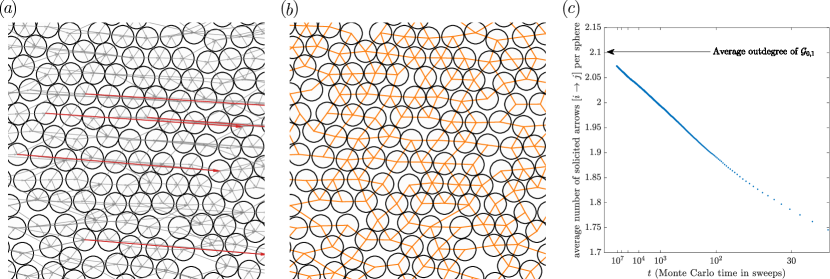
Figure 6: ECMC constraint graphs for $\mathcal{C}^{256}$ (see Section 3.2 for definition). (a): $\mathcal{G}^{(3)}$ for this configuration (detail), with highlighted non-local arrows. (b): $\mathcal{G}^{256}$ (same detail), obtained from $\mathcal{G}^{(3)}$ through fourth-order pruning followed by symmetrization. (c): Number of solicited arrows in $\mathcal{G}^{256}$ in a long cell-based ECMC run, compared to its average outdegree.

3.2 Validation

Our programs apply to arbitrary density $\eta=N\pi\sigma^{2}/L^{2}$ and linear size $L$ of the periodic square box (with $N=M^{2}$). We provide sets of configurations and constraint graphs for validation and benchmarking. One such set consists in a configuration $\mathcal{C}^{256}$ at $M=256$, and for $\eta=0.708$ and a fourth-order symmetrized constraint graph $\mathcal{G}^{256}$. Where applicable, the number of active spheres varies as $k=1,2,4,\ldots,k^{\max}$ and the number of threads as $n_{\iota}=1,2,3,\ldots,n_{\iota}^{\max}$. For fixed $k$ and $n_{\iota}$, there are $n_{\text{run}}$ runs that vary $h$ and $h^{\prime}$.

Constraint-graph validation

Constraint graphs are generated in the Setup.sh script. The GraphValidateCellECMC test performs cell-based ECMC derived from CellECMC.f90  [3, 23], where spheres are assigned to local cells and neighborhood-cell searches identify possible liftings. Cell-based ECMC must exclusively solicit liftings accounted for in $\mathcal{G}$. The GraphValidateCellECMC test also records the sweep (lifting per sphere) at which an arrow $[i\!\!\to\!\!j]\in\mathcal{G}$ is first solicited in a lifting and compares the time evolution of the average number of solicited arrows with its average outdegree. The $\mathcal{G}^{256}$ constraint graph passes the validation test with $t=2\!\times\!10^{7}$ sweeps. The outdegree of $\mathcal{G}^{256}$ is $2.1$, and $98.7$ % of its arrows are solicited during the test. Logarithmic extrapolation (with $1/{(\ln{t})}^{\alpha}$, $\alpha=1.7$) suggests that $\mathcal{G}^{256}$ essentially agrees with $\mathcal{G}^{\min}$ (see Fig. 6c). Use of $\mathcal{G}^{256}$ rather than $\mathcal{G}^{(3)}$ speeds up ECMC, but further performance gains through additional pruning are certainly extremely limited.

Validation of Algs 2 and 6

Our implementations of Algorithms 2 and 6 are modified as discussed in Remark 7. Runs compute the set $\mathcal{L}_{t^{*}}$ to the earliest horizon-violation time $t^{*}$ (with $t^{*}=h^{\prime}$ if the run concludes successfully). The PValidateECMC.sh test first advances $\mathcal{C}^{256}=\mathcal{C}_{t=0}$ to a random breakpoint $h$ (using $\mathcal{L}^{\text{ref}}$). Each test run is in the interval $[h,h^{\prime}]$, where $h^{\prime}$ is randomly chosen. To pass the validation test, $\mathcal{L}_{t^{*}}$ must for each run agree with $\mathcal{L}^{\text{ref}}$(see Section 4 for details of scripts used). Algorithm 2 passes the PValidateECMC.sh test with $n_{\text{run}}=1\!\times\!10^{3}$ for $k^{\max}=8192$.

Our x86 computer has two Xeon Gold 6230 CPUs with variable frequency from $2.1$ GHz to $3.9$ GHz, each with $20$ cores and $40$ hardware threads. We use OpenMP directives to restrict all threads to a single x86 CPU. We consider again $\mathcal{C}^{256}=\mathcal{C}_{t=0}$ as the initial configuration, and then run the program from $h$ to $h^{\prime}$. On our x86 CPU, Algorithm 6 passes the CValidateECMC.sh test with $n_{\text{run}}=1\!\times\!10^{3}$, $k^{\max}=8192$ and $n^{\max}_{\iota}=40$.

On our ARM CPU (Nvidia Jetson with Cortex A57 CPU (at $1.43$ GHz) with four cores and four hardware threads), we again consider $\mathcal{C}^{256}=\mathcal{C}_{t=0}$ as initial configuration. For the same system parameters as above, Algorithm 6 passes the CValidateECMC.sh test with $n_{\text{run}}=1\!\times\!10^{3}$, $k^{\max}=8192$ and $n^{\max}_{\iota}=4$. The ARM architecture allows dynamic re-ordering of operations, and the separate validation test more severely scrutinizes thread interactions than for the x86 CPU.

On both CPUs, Algorithm 6 passes the CValidateECMC.sh test with the following choices of memory_order directives:

memory_order_relaxed. This most permissive memory ordering of the C++ memory model imposes no constraints on compiler optimization or dynamic re-ordering of operations by the processors, and only guarantees the atomic nature of the CAS operation. Such re-orderings are more aggressive on ARM CPUs than on x86 CPUs. This memory ordering does not guarantee that the statements constituting the lock-less lock are executed as required (see Remark 12).

memory_order_seq_cst for all memory operations on the tag attribute. This directive imposes the sequential-consistency model (see Remark 12) for each access of the tag attribute. It slows down the code by $40$% compared to the memory_order_relaxed directive.

memory_order_acquire on load, memory_order_release on store. This directive implies “acquire–release” semantics on the tag attribute. It imposes a lock-free exchange at each operation on the tag attribute, so that all variables, including positions and local times, are synchronized between threads during tag access. CAS remains memory_order_seq_cst. This directive maintains speed compared to memory_order_relaxed, yet provides better guarantees on the propagation of variable modification between threads. MultiThreadECMC.cc compiles by default with this directive.

3.3 Benchmarks for Algorithm 6 (x86 and ARM)

Algorithm 6 is modified as discussed in Remark 7 (program execution continues in spite of horizon violations) and used for large values of $h^{\prime}$. This measures the net cost of steady-state thread interaction, without taking into account thread-setup times. We report here on results of the BenchmarkECMC.sh script for $\mathcal{C}^{256}$ as an initial configuration and $\mathcal{G}^{256}$ with $k=80$ active spheres. The number of threads varies as $n_{\iota}=1,2,3,\ldots,n_{\iota}^{\max}$, with $n_{\text{run}}=20$.

On our x86 CPU (see Section 3.2), the BenchmarkECMC.sh script is parametrized with $n_{\iota}^{\max}=40$. The benchmark speed increases roughly linearly up to $20$ threads (reaching a speed-up of $12$ for $20$ threads), and then keeps improving more slowly with a maximum for $40$ threads at a speed-up of $16$ and an absolute speed of $\sim 1.7\!\times\!10^{12}$ events/hour (see Fig. 7). The variable frequency of Xeon processors under high load may contribute to this complex behavior. On a single thread, our program runs $2.4$ times slower than an unthreaded code, due to the eliminated overhead from threading constructs. The original CellECMC.f90 cell-based production code generates $3\!\times\!10^{10}$ events/hour. The use of a constraint graph, rather than a cell-based search, thus improves performance by almost an order of magnitude, if the set-up of $\mathcal{G}$ is not accounted for.

On our ARM CPU, the BenchmarkECMC.sh script is parametrized with $n_{\iota}^{\max}=4$. The benchmark speed increases as the number of threads, reaching a speed-up of $4.0$ for $n_{\iota}=4$. The absolute speed is about seven times smaller than for our x86 CPU for a comparable number of threads, as may be expected for a low-power processor designed for use in mobile phones.

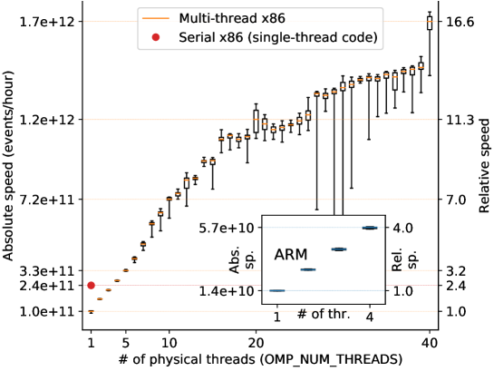
Figure 7: Output of the BenchmarkECMC.sh script for Algorithm 6 (five-number summary of $20$ runs) for $k=80$ on an x86 CPU with $20$ cores and $1,\ldots,40$ threads, and for serial code that processes active chains sequentially. Inset: Output of the script for a four-core ARM CPU.

3.4 Birthday problem, full ECMC, multi-CPU extensions

In this section, we treat some practical aspects for the use of Algorithm 6.

Birthday problem

We analyze multithreaded ECMC in terms of the (generalized) birthday problem, which considers the probability $p$ that two among $k^{\prime}$ integers (modeling individuals) sampled from a discrete uniform distribution in the set $\{1,2,\ldots,N^{\prime}\}$ (modeling birthdays) are the same. For large $N^{\prime}$, $p\sim[1-\exp{(-k^{\prime 2}/(2N^{\prime}))}]$ [28], which is small if $k^{\prime}\lesssim\sqrt{N^{\prime}}$. At constant density $\eta$, sphere radius $\sigma$, velocity $\mathbf{v}$, and time interval $h^{\prime}-h$, each active chain $\iota$ is restricted to a region of constant area, whereas the total area of the simulation box is $\eta N$. We may suppose that the $k$ active spheres are randomly positioned in the simulation box broken up into a grid of $\propto N$ constant-area cells. For $k\lesssim\sqrt{N}$, we expect the probability that one of these cells contains two active spheres to remain constant for $N\to\infty$, and therefore also the probability of an update-order violation for constant $h^{\prime}-h$.

Restarts

Our algorithms reproduce output of Algorithm 1 only if they do not abort. In production code, the effects of horizon violations will have to be repaired. Two strategies appear feasible. First, the algorithm may restart the run from a copy of $\{\mathcal{C}_{h},\mathcal{A}_{h}\}$ at the initial breakpoint $h$, and choose a smaller breakpoint $h^{\prime\prime}$, for example the time of abort. The successful termination of this restart is not guaranteed, as the individual threads may organize differently. Second, the time evolution may be reconstructed from $\mathcal{L}_{t^{*}}$ to the earliest horizon-violation time $t^{*}$ (see Remark 7), and $t^{*}$ may then be used as the subsequent initial breakpoint. Besides an efficient restart strategy, a multithreaded production code will also need an efficient parallel algorithm for computing $\mathcal{G}$ after a change of $\mathbf{v}$.

Multi-CPU implementations

Algorithm 6 is spelled out for a single shared-memory CPU and for threads that may access attributes of all spheres (see statement $10\iota$ in Algorithm 5 and Remark 11). However, thread interactions are local and immutable in between breakpoints (as evidenced by the constraint graphs). This invites generalizations of the algorithm to multiple CPUs (each of them with many threads). Most simply, two CPUs could administer disjoint parts of the constraint graph, for example with interface vertices doubled up on both of them (see Fig. 8). In this way, an active sphere arriving at an interface would simply be copied out to the neighboring CPU. The generalization to multiple CPUs appears straightforward.

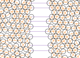
Figure 8: A constraint graph doubled up for a multi-CPU implementation of Alg. 6 (detail of $\mathcal{C}^{256}$ configuration shown). Interface vertices appear on both sides.

4 Available computer code

All implemented algorithms and used scripts that are made available on GitHub in ParaSpheres, the public repository, which is part of a public GitHub organization. Code is made available under the GNU GPLv3 license (for details see the LICENSE file).

The repository can be forked (that is, copied to an outside user’s own public repository) and from there studied, modified and run in the user’s local environment. Users may contribute to the ParaSpheres project via pull requests (see the README.md and CONTRIBUTING.md files for instructions and guidelines). All communication (bug reports, suggestions) take place through GitHub “Issues”, that can be opened in the repository by any user or contributor, and that are classified in GitHub projects.

Implemented algorithms

The following programs are located in the directory tree under their language (F90, Python or CPP) and in similarly named subdirectories, that all contain README files for further details. Some of the longer programs are split into modules.

Code/Directory Algorithm / Usage CellECMC.f90 Cell-based production ECMC [3] GenerateG3.py Generate $\mathcal{G}^{(3)}$ (Section 3.1) PruneG.py Prune $\mathcal{G}$ (Section 3.1) GraphValidateCellECMC.cc Validate $\mathcal{G}$ against cell-based ECMC GlobalTimeECMC.py Alg. 1 (Section 2.1) SingleThreadLocalTimeECMC.py Alg. 2 (Section 2.2) SequentialMultiThreadECMC.py Alg. 5 (Section 2.3) MultiThreadECMC.cc Alg. 6 (Section 2.4)

Scripts and validation suites

The Scripts directory provides the following bash scripts to compile and run groups of programs and to reproduce all our results:

Script Summary of usage Setup.sh Prepare $\mathcal{C}_{t=0}$, $\mathcal{G}$, $\mathcal{L}^{\text{ref}}$ SequentialC4.sh Test suite for Alg. 5 with $N=4$ SequentialC5.sh Test suite for Alg. 5 with $N=5$ (see Remark 12) Ordering.sh Test suite for Alg. 6 with $N=5$ (see Remark 12) ValidateG.sh Validate constraint graph PValidateECMC.sh Validate Alg. 2 against $\mathcal{L}^{\text{ref}}$ CValidateECMC.sh Validate Alg. 6 against $\mathcal{L}^{\text{ref}}$ BenchmarkECMC.sh Benchmark MultiThreadECMC.cc, generate Fig. 7

In the Setup.sh script, CellECMC.f90 first produces an equilibrated sample $\mathcal{C}_{0}$. It then generates $\mathcal{G}^{(3)}$ with GenerateG3.py, and runs PruneG.py to output $\mathcal{G}$. Finally, it runs GlobalTimeECMC.py for each set $\mathcal{A}_{0}$, in order to generate generate several $\mathcal{L}^{\text{ref}}$. The ValidateG.sh script runs cell-based ECMC, using GraphValidateCellECMC.cc, and verifies that all liftings are accounted for in $\mathcal{G}$. It also tracks the solicitation of arrows as a function of time. The PValidateECMC.sh script validates SingleThreadLocalTimeECMC.py by comparing the sets of liftings with $\mathcal{L}^{\text{ref}}$from Setup.sh. The CValidateECMC.sh script does the same for MultiThreadECMC.cc The BenchmarkECMC.sh script benchmarks MultiThreadECMC.cc for different numbers of threads. The test suites are concerned with small-$N$ configurations.

5 Conclusions and outlook

In this paper, we presented an event-driven multithreaded ECMC algorithm for hard spheres which enforces thread synchronization at infrequent breakpoints only. Between breakpoints, spheres carry and update local times. Possible inconsistencies are locally detected through a horizon condition. Within ECMC, our method avoids the scheduling problem that has historically plagued event-driven molecular dynamics. This is possible because in ECMC only few spheres move at any moment, and all have the same velocity. Conflicts are thus exceptional, and little information is exchanged between threads. We relied the generalized birthday problem to show that our algorithm remains viable up to a number of threads that grows as the square root of the number of spheres, a setting relevant for the simulation of millions of spheres for modern commodity servers with $\sim 100$ threads. The mapping of Algorithm 5 onto an absorbing Markov chain allowed us to prove its correctness (for a given lifted initial configuration), and to rigorously analyze side effects of code re-orderings in the multithreaded C++ code.

Our algorithm is presently implemented between two global breakpoint times, where it achieves considerable speed-up with respect to sequential ECMC. Generalization for a full practical multithreaded ECMC code that greatly outperforms cell-based algorithms appear within reach. It is still a challenge to understand whether multithreaded ECMC applies to general interacting-particle systems.

References

- [1] E. P. Bernard, W. Krauth, D. B. Wilson, Event-chain Monte Carlo algorithms for hard-sphere systems, Phys. Rev. E 80 (2009) 056704. arXiv:0903.2954, doi:10.1103/PhysRevE.80.056704.
- [2] M. Michel, S. C. Kapfer, W. Krauth, Generalized event-chain Monte Carlo: Constructing rejection-free global-balance algorithms from infinitesimal steps, J. Chem. Phys. 140 (5) (2014) 054116. arXiv:1309.7748, doi:10.1063/1.4863991.
- [3] E. P. Bernard, W. Krauth, Two-Step Melting in Two Dimensions: First-Order Liquid-Hexatic Transition, Phys. Rev. Lett. 107 (2011) 155704. arXiv:1102.4094, doi:10.1103/PhysRevLett.107.155704.
- [4] S. C. Kapfer, W. Krauth, Two-Dimensional Melting: From Liquid-Hexatic Coexistence to Continuous Transitions, Phys. Rev. Lett. 114 (2015) 035702. arXiv:1406.7224, doi:10.1103/PhysRevLett.114.035702.
- [5] M. Hasenbusch, S. Schaefer, Testing the event-chain algorithm in asymptotically free models, Phys. Rev. D 98 (2018) 054502. arXiv:1806.11460, doi:10.1103/PhysRevD.98.054502.
- [6] E. P. Bernard, W. Krauth, Addendum to “Event-chain Monte Carlo algorithms for hard-sphere systems”, Physical Review E 86 (1) (2012) 017701. arXiv:1111.6964, doi:10.1103/physreve.86.017701.
- [7] S. C. Kapfer, W. Krauth, Irreversible Local Markov Chains with Rapid Convergence towards Equilibrium, Phys. Rev. Lett. 119 (2017) 240603. arXiv:1705.06689, doi:10.1103/PhysRevLett.119.240603.
- [8] M. F. Faulkner, L. Qin, A. C. Maggs, W. Krauth, All-atom computations with irreversible Markov chains, The Journal of Chemical Physics 149 (6) (2018) 064113. arXiv:1804.05795, doi:10.1063/1.5036638.
- [9] J. Harland, M. Michel, T. A. Kampmann, J. Kierfeld, Event-chain Monte Carlo algorithms for three- and many-particle interactions, EPL (Europhysics Letters) 117 (3) (2017) 30001. arXiv:1611.09098, doi:10.1209/0295-5075/117/30001.
- [10] N. Metropolis, A. W. Rosenbluth, M. N. Rosenbluth, A. H. Teller, E. Teller, Equation of State Calculations by Fast Computing Machines, J. Chem. Phys. 21 (1953) 1087–1092. doi:10.1063/1.1699114.
- [11] B. J. Alder, T. E. Wainwright, Phase Transition for a Hard Sphere System, J. Chem. Phys. 27 (1957) 1208–1209. doi:10.1063/1.1743957.
- [12] B. J. Alder, T. E. Wainwright, Studies in Molecular Dynamics. I. General Method, J. Chem. Phys. 31 (1959) 459–466. doi:10.1063/1.1730376.
- [13] D. C. Rapaport, The Event Scheduling Problem in Molecular Dynamic Simulation, Journal of Computational Physics 34 (1980) 184–201. doi:10.1016/0021-9991(80)90104-7.
- [14] M. Isobe, Hard sphere simulation in statistical physics methodologies and applications, Molecular Simulation 42 (16) (2016) 1317–1329. doi:10.1080/08927022.2016.1139106.
- [15] B. D. Lubachevsky, Simulating billiards serially and in parallel, International Journal in Computer Simulation 2 (1992) 373–411.
- [16] B. Lubachevsky, Several unsolved problems in large-scale discrete event simulations, ACM SIGSIM Simulation Digest 23 (1993) 60–67. doi:10.1145/174134.158467.
- [17] A. G. Greenberg, B. D. Lubachevsky, I. Mitrani, Superfast parallel discrete event simulations, ACM Transactions on Modeling and Computer Simulation (TOMACS) 6 (2) (1996) 107–136.
- [18] A. T. Krantz, Analysis of an efficient algorithm for the hard-sphere problem, ACM Trans. Model. Comput. Simul. 6 (3) (1996) 185–209. doi:10.1145/235025.235030.
- [19] M. Marin, Billiards and related systems on the bulk-synchronous parallel model, in: Proceedings 11th Workshop on Parallel and Distributed Simulation, 1997, pp. 164–171. doi:10.1109/PADS.1997.594602.
- [20] S. Miller, S. Luding, Event-driven molecular dynamics in parallel, Journal of Computational Physics 193 (1) (2004) 306 – 316. arXiv:physics/0302002, doi:10.1016/j.jcp.2003.08.009.
- [21] P. Diaconis, S. Holmes, R. M. Neal, Analysis of a nonreversible Markov chain sampler, Annals of Applied Probability 10 (2000) 726–752.
- [22] D. A. Levin, Y. Peres, E. L. Wilmer, Markov Chains and Mixing Times, American Mathematical Society, 2008.
- [23] M. Engel, J. A. Anderson, S. C. Glotzer, M. Isobe, E. P. Bernard, W. Krauth, Hard-disk equation of state: First-order liquid-hexatic transition in two dimensions with three simulation methods, Phys. Rev. E 87 (2013) 042134. arXiv:1211.1645, doi:10.1103/PhysRevE.87.042134.
- [24] Lamport, How to Make a Multiprocessor Computer That Correctly Executes Multiprocess Programs, IEEE Transactions on Computers C-28 (9) (1979) 690–691. doi:10.1109/tc.1979.1675439.
- [25] H. J. Boehm, L. Crowl, C++ atomic types and operations, http://www.open-std.org/jtc1/sc22/wg21/docs/papers/2007/n2427.html (2009).
- [26] S. C. Kapfer, W. Krauth, Sampling from a polytope and hard-disk Monte Carlo, Journal of Physics: Conference Series 454 (1) (2013) 012031. arXiv:1301.4901, doi:10.1088/1742-6596/454/1/012031.
- [27] K. Fukuda, B. Gärtner, M. Szedlák, Combinatorial redundancy detection, Annals of Operations Research 265 (1) (2016) 47–65. doi:10.1007/s10479-016-2385-z.
- [28] F. H. Mathis, A generalized birthday problem, SIAM Review 33 (2) (1991) 265–270. doi:10.1137/1033051.