Joint Radar Target Detection and Parameter Estimation with MIMO OTFS

Abstract

Motivated by future automotive applications, we study the joint target detection and parameter estimation problem using orthogonal time frequency space (OTFS), a digital modulation format robust to time-frequency selective channels. Assuming the transmitter is equipped with a mono-static MIMO radar, we propose an efficient maximum likelihood based approach to detect targets and estimate the corresponding delay, Doppler, and angle-of-arrival parameters. In order to reduce the computational complexity associated to the high-dimensional search, our scheme proceeds in two steps, i.e., target detection and coarse parameter estimation followed by refined parameter estimation. Interestingly, our numerical results demonstrate that the proposed scheme is able to identify multiple targets if they are separated in at least one domain out of three (delay, Doppler, and angle), while achieving the Cramér-Rao lower bound for the parameter estimation.

I Introduction

The multiple-input multiple-output (MIMO) radar has been extensively studied and has been shown to improve the resolution, i.e., the ability to distinguish multiple targets, thanks to an additional spatial dimension (see, e.g., [1]). A careful design of beamforming (BF), or power allocation along angular directions, is crucial to achieve accurate radar detection and parameter estimation performance. This is particularly relevant to automotive radar [2] operating over millimeter wave (mmWave) frequency bands as high propagation loss must be compensated by proper BF, or more generally beam alignment both at transmitter and receiver sides (see e.g. [3] and references therein). Note that in a mono-static radar system with co-located transmitter and receiver, transmit and receive antennas are calibrated such that their beam patterns are consistent, i.e., “look in the same direction”. Moreover, BF at the radar transmitter might be adaptive, depending on different operating phases (see e.g., [4, 5] and references therein). Namely, the transmitted power shall be allocated to wider angular sectors during a target detection/search phase, while narrow and distinct beams, each focused on the detected target, shall be used to minimize “multi-target” interference in a tracking phase [1, 6, 7]. During the target detection phase, a non-trivial tradeoff appears. On one hand, a wider angular sector coverage enables to detect multiple targets if the received backscattered power is high enough. On the other hand, a more directional BF grants a higher received signal-to-noise ratio (SNR), at the cost of a time-consuming search over narrower angular sectors.

As an extension of our previous work [8], this paper studies the joint problem of target detection and parameter estimation with a MIMO mono-static radar adopting orthogonal time frequency space (OTFS), i.e., a multi-carrier communication waveform recently proposed in [9]. The use of communication waveforms for radar has been motivated by the joint radar and communication paradigm, where two functions are implemented by sharing the same resources and the same waveform (see e.g. [10, 11, 12] and references therein). In particular, delay and Doppler estimation based on OTFS has been also considered in [13], where the authors propose a matched filter based approach to estimate the parameters within discrete delay-Doppler grids. In this work, we assume that the coverage is wide enough such that multiple targets could be located at different angles within the same beam, contrary to the time-consuming beam sweeping considered in [8]. Under this setup, we aim to find an efficient method for target detection and delay, Doppler, and angle of arrival (AOA) estimation under practical OTFS system constraints related to the underlying physical channel, explained within the paper.

Our main contributions are two-fold: i) we propose an efficient two-step approach for joint target detection and four-dimensional parameter estimation. In order to reduce the computational complexity associated to the high-dimensional search, our maximum likelihood (ML) based scheme first performs coarse estimation and target detection, and then refines further the parameter estimation; ii) simulation results demonstrate that our proposed approach can identify multiple targets if they are separated in at least one domain out of three (delay, Doppler, and angle), while achieving the Cramér-Rao Lower Bound (CRLB) for the parameter estimation.

The paper is organized as follows. In Section II, we introduce the physical model (of the channel) and the OTFS input-output relation. Section III describes our proposed joint detection and parameters estimation algorithm, together with the definition of the CRLB. After showing the simulation results in Section IV, Section V concludes the paper.

II Physical model

We consider joint radar detection and parameter estimation in a system operating over a channel bandwidth $B$ at the carrier frequency $f_{c}$. We assume that a transmitter is equipped with a mono-static MIMO radar with $N_{a}$ antennas and operating in full duplex. Wide angular sectors are illuminated by the transmit beam and the receiver processes the backscattered signal to identify the presence of targets within the beam, together with the estimation of parameters of interest such as range, velocity, and angular position.

In order to take advantage of the available bandwidth, automotive radar systems typically operate at mmWave carrier frequencies [2]. At mmWave, although the number of antennas may be very large, the number of radio frequency (RF) chains is limited due to the difficulty of implementing a full per-antenna RF chain (including A/D conversion, modulation, and amplification) in a small form factor and highly integrated technology, for large signal bandwidths. Full digital BF is thus precluded, while hybrid digital-analog BF schemes is typically adopted (see, e.g., [15] and references therein). Targeting possible mmWave automotive applications, we consider a number of RF chains smaller than the number of antennas, i.e., $N_{\rm rf}\leq N_{a}$.

We consider a point target model such that each target can be represented through its line-of-sight (LoS) path only [16, 17]. By letting $\phi\in[-\frac{\pi}{2},\frac{\pi}{2}]$ be the steering angle, the transmitter and receiver arrays are given by ${\bf a}(\phi)$ and ${\bf b}(\phi)$, where ${\bf b}(\phi)=(b_{1}(\phi),\dots,b_{N_{a}}(\phi))\in\mbox{\bb C}^{N_{a}}$ denotes the uniform linear array response vector of the radar receiver, given by

$$b_{n}(\phi) =e^{j(n-1)\pi\sin(\phi)},\;\;n=1,\dots,N_{a}\,,$$ (1)

and ${\bf a}(\phi)$ is defined similarly (at the radar transmitter). The channel is modeled as a $P$-tap time-frequency selective channel of dimension $N_{a}\times N_{a}$ given by [18]

$${\bf H}(t,\tau)=\sum_{p=1}^{P}h_{p}{\bf b}(\phi_{p}){\bf a}^{\scriptscriptstyle\mathsf{H}}(\phi_{p})\delta(\tau-\tau_{p})e^{j2\pi\nu_{p}t}\,,$$ (2)

where $(\cdot)^{\scriptscriptstyle\mathsf{H}}$ denotes the Hermitian (conjugate and transpose) operation, $P$ is the number of targets, $h_{p}$ is a complex channel gain including the pathloss (PL) of the path component, $\nu_{p}=\frac{2v_{p}f_{c}}{c}$, $\tau_{p}=\frac{2r_{p}}{c}$ denote the corresponding round-trip Doppler shift, delay associated to the $p$-th target, respectively.

II-A OTFS Input Output Relation

We consider OTFS with $M$ subcarriers of bandwidth $\Delta f$ each, such that the total bandwidth is given by $B=M\Delta f$. We let $T$ denote the symbol time, and the OTFS frame duration is $NT$, imposing $T\Delta f=1$. By following the standard derivation of the input-output relation of OTFS (see, e.g., [9, 8]), data symbols $\left\{x_{k,l}\right\}$, for $k=0,\dots,N-1$ and $l=0,\dots,M-1$ belonging to any constellation, are arranged in an $N\times M$ two-dimensional grid referred to as the Doppler-delay domain, i.e., $\Gamma=\left\{\left({k}/{NT},{l}/{M\Delta f}\right)\right\}$ for $k=0,\dots,N-1$ and $l=0,\dots,M-1$. The transmitter first applies the inverse symplectic finite Fourier transform (ISFFT) to convert data symbols $\{x_{k,l}\}$ into a block of samples $\{X[n,m]\}$ in the dual domain, referred to as the time-frequency domain, thus

$$X[n,m]=\sum_{k=0}^{N-1}\sum_{l=0}^{M-1}x_{k,l}e^{j2\pi\left(\frac{nk}{N}-\frac{ml}{M}\right)},$$ (3)

for $n=0,\ldots,N-1$ and $m=0,\ldots,M-1$. Then, it generates the continuous-time signal

$$s(t)=\sum_{n=0}^{N-1}\sum_{m=0}^{M-1}X[n,m]g_{\rm tx}(t-nT)e^{j2\pi m\Delta f(t-nT)}\,,$$ (4)

where $X[n,m]$ denotes the symbol sent at time $n$ over subcarrier $m$, satisfying the average power constraint $\mbox{\bb E}[|X[n,m]|^{2}]\leq{P_{\rm avg}}/{N_{a}}$. For simplicity, we consider that the same symbol stream $\{X[n,m]\}$ is repeated over all RF chains. After transmission over the channel defined in (2), the continuous received signal without noise including BF is

$${\bf r}(t)=\sum_{p=0}^{P-1}h_{p}{\bf b}(\phi_{p}){\bf a}^{\scriptscriptstyle\mathsf{H}}(\phi_{p}){\bf f}_{\mathrm{BF}}s(t-\tau_{p})e^{j2\pi\nu_{p}t}\,,$$ (5)

where ${\bf f}_{\mathrm{BF}}$ is a generic BF vector of dimension $N_{a}\times 1$. Typical BF designs can be found, e.g., in [4, 19].

The output of the receiver filter-bank adopting a generic receive shaping pulse $g_{\rm rx}(t)$ is given in (II-A),

$${\bf y}(t ,f)=\int{\bf r}(t^{\prime})g^{*}_{\rm rx}(t^{\prime}-t)e^{-j2\pi ft^{\prime}}dt^{\prime}=\int_{t^{\prime}}g^{*}_{\rm rx}(t^{\prime}-t)\sum_{p=0}^{P-1}h_{p}{\bf b}(\phi_{p}){\bf a}^{\scriptscriptstyle\mathsf{H}}(\phi_{p}){\bf f}_{\mathrm{BF}}s(t^{\prime}-\tau_{p})e^{j2\pi\nu_{p}t^{\prime}}e^{-j2\pi ft^{\prime}}dt^{\prime}$$

$$=\sum_{p,n^{\prime},m^{\prime}}h_{p}{\bf b}(\phi_{p}){\bf a}^{\scriptscriptstyle\mathsf{H}}(\phi_{p}){\bf f}_{\mathrm{BF}}X[n^{\prime},m^{\prime}]\int_{t^{\prime}}g^{*}_{\rm rx}(t^{\prime}-t)g_{\rm tx}(t^{\prime}-\tau_{p}-n^{\prime}T)e^{j2\pi m^{\prime}\Delta f(t^{\prime}-\tau_{p}-n^{\prime}T)}e^{j2\pi(\nu_{p}-f)t^{\prime}}dt^{\prime}$$ (6)

and, by sampling at $t=nT$ and $f=m\Delta f$, we obtain

$${\bf y}[n,m] ={\bf y}(t,f)|_{t=nT,f=m\Delta f}$$

$$=\sum_{n^{\prime}=0}^{N-1}\sum_{m^{\prime}=0}^{M-1}X[n^{\prime},m^{\prime}]{\bf h}_{n,m}[n^{\prime},m^{\prime}]\,,$$ (7)

where the time-frequency domain channel ${\bf h}_{n,m}[n^{\prime},m^{\prime}]$ is given in (8),

$${\bf h}_{n,m}[n^{\prime},m^{\prime}]=\sum_{p=0}^{P-1}h^{\prime}_{p}{\bf b}(\phi_{p}){\bf a}^{\scriptscriptstyle\mathsf{H}}(\phi_{p}){\bf f}_{\mathrm{BF}}C_{g_{\rm tx},g_{\rm rx}}((n-n^{\prime})T-\tau_{p},(m-m^{\prime})\Delta f-\nu_{p})e^{j2\pi n^{\prime}T\nu_{p}}e^{-j2\pi m\Delta f\tau_{p}}$$ (8)

by defining the cross ambiguity function $C_{u,v}(\tau,\nu)\stackrel{{\scriptstyle\Delta}}{{=}}\int_{-\infty}^{\infty}u(s)v^{*}(s-\tau)e^{-j2\pi\nu s}ds$ as in [20], letting $h^{\prime}_{p}=h_{p}e^{j2\pi\nu_{p}\tau_{p}}$, and imposing the term $e^{-j2\pi mn^{\prime}\Delta fT}=1$, $\forall n^{\prime},m$, which is always true under the hypothesis $T\Delta f=1$. Since $X[n,m]$ is generated via ISFFT, the received signal in the delay-Doppler domain is obtained by the application of the symplectic finite Fourier transform (SFFT)

$${\bf y}[k,l]\!=\!\sum_{n,m}\frac{{\bf y}[n,m]}{NM}e^{j2\pi\left(\frac{ml}{M}-\frac{nk}{N}\right)}\!\!=\!\!\sum_{k^{\prime},l^{\prime}}x_{k^{\prime},l^{\prime}}{\bf g}_{k,k^{\prime}}\left[l,l^{\prime}\right],$$ (9)

where the inter-symbol interference (ISI) coefficient of the Doppler-delay pair $\left[k^{\prime},l^{\prime}\right]$ seen by sample $\left[k,l\right]$ is given by

$${\bf g}_{k,k^{\prime}}\left[l,l^{\prime}\right]=\sum_{p}h_{p}^{\prime}{\bf b}(\phi_{p}){\bf a}^{\scriptscriptstyle\mathsf{H}}(\phi_{p}){\bf f}_{\mathrm{BF}}\Psi^{p}_{k,k^{\prime}}[l,l^{\prime}]\,,$$ (10)

with $\Psi^{p}_{k,k^{\prime}}[l,l^{\prime}]$ defined in (11).

$$\Psi^{p}_{k,k^{\prime}}[l,l^{\prime}]=\!\!\!\sum_{n,n^{\prime},m,m^{\prime}}\!\!\!\frac{C_{g_{\rm rx},g_{\rm tx}}((n-n^{\prime})T-\tau_{p},(m-m^{\prime})\Delta f-\nu_{p})}{NM}e^{j2\pi n^{\prime}T\nu_{p}}e^{-j2\pi m\Delta f\tau_{p}}e^{j2\pi\left(\frac{n^{\prime}k^{\prime}}{N}-\frac{m^{\prime}l^{\prime}}{M}\right)}e^{-j2\pi\left(\frac{nk}{N}-\frac{ml}{M}\right)}$$ (11)

 

Note that a simplified version of $\Psi^{p}_{k,k^{\prime}}[l,l^{\prime}]$ obtained by approximating the cross ambiguity function can be found in [8].

At this point, let’s define

$${\bf G}_{p}(\tau_{p},\nu_{p},\phi_{p})\triangleq\left({\bf b}\left(\phi_{p}\right){\bf a}^{\scriptscriptstyle\mathsf{H}}(\phi_{p}){\bf f}_{\mathrm{BF}}\right)\otimes\hbox{\boldmath$\Psi$}^{p}\,,$$ (12)

where $\otimes$ is the Kronecker product, as the $N_{a}NM\times NM$ matrix obtained by multiplying $\hbox{\boldmath$\Psi$}^{p}$ by a different coefficient of $\left({\bf b}\left(\phi_{p}\right){\bf a}^{\scriptscriptstyle\mathsf{H}}(\phi_{p}){\bf f}_{\mathrm{BF}}\right)$. Thus, by stacking ${\bf X}$ into a $NM$-dimensional vector ${\bf x}$ and defining an output vector ${\bf y}$ of dimension $NMN_{a}\times 1$, the received signal in the presence of noise is given by

$${\bf y}=\sum_{p=0}^{P-1}\left[h^{\prime}_{p}{\bf G}_{p}(\tau_{p},\nu_{p},\phi_{p})\right]{\bf x}+{\bf w}\,,$$ (13)

where ${\bf w}$ denotes the additive white Gaussian noise (AWGN) vector with independent and identically distributed entries of zero mean and variance $\sigma_{w}^{2}$. The problem reduces to detect $P$ targets and estimate the $4P$ associated parameters (complex channel coefficient, Doppler, delay, and angle) from the $N_{a}MN$-dimensional received signal.

III Joint Detection and Parameters Estimation

We wish to estimate the set of four parameters $\hbox{\boldmath$\theta$}=\{h^{\prime}_{p},\phi_{p},\tau_{p},\nu_{p}\}\in{\cal T}^{P}$, with ${\cal T}=\mbox{\bb C}\times\mbox{\bb R}\times\mbox{\bb R}\times\mbox{\bb R}$. We define the ML function as

$$l({\bf y}|\hbox{\boldmath$\theta$},{\bf x}) =\left|{\bf y}-\sum_{p}h^{\prime}_{p}{\bf G}_{p}{\bf x}\right|^{2},$$ (14)

where we use the short hand notation ${\bf G}_{p}\triangleq{\bf G}(\tau_{p},\nu_{p},\phi_{p})$. The ML solution is given by

$$\hat{\hbox{\boldmath$\theta$}}={\hbox{arg}}\min_{\hbox{\boldmath$\theta$}\in{\cal T}^{P}}l({\bf y}|\hbox{\boldmath$\theta$},{\bf x}).$$ (15)

For a fixed set of $\{\phi_{p},\tau_{p},\nu_{p}\}$, the ML estimator of $\{h^{\prime}_{p}\}$ is given by solving the following set of equations

$${\bf x}^{\scriptscriptstyle\mathsf{H}}{\bf G}^{\scriptscriptstyle\mathsf{H}}_{p}\left(\sum_{q=0}^{P-1}h^{\prime}_{q}{\bf G}_{q}\right){\bf x} ={\bf x}^{\scriptscriptstyle\mathsf{H}}{\bf G}^{\scriptscriptstyle\mathsf{H}}_{p}{\bf y},\;\;\;p=0,\dots,P-1.$$ (16)

By plugging (16) into (14), it readily follows that minimizing $l({\bf y}|\hbox{\boldmath$\theta$},{\bf x})$ reduces to maximize

$$l_{2}({\bf y}|\hbox{\boldmath$\theta$},{\bf x}) =\sum_{p}h^{\prime}_{p}{\bf y}^{\scriptscriptstyle\mathsf{H}}{\bf G}_{p}{\bf x}$$

$$=\sum_{p}S_{p}(\tau_{p},\nu_{p},\phi_{p})-I_{p}(\{h^{\prime}_{q}\}_{q\neq p},\hbox{\boldmath$\theta$})\,,$$ (17)

where $S_{p}(\tau_{p},\nu_{p},\phi_{p})$ and $I_{p}(\{h^{\prime}_{q}\}_{q\neq p},\hbox{\boldmath$\theta$})$ ($S_{p}$ and $I_{p}$ in short hand notation) denote the useful signal and the interference term for target $p$, given respectively by

$$S_{p}=\frac{|{\bf y}^{\scriptscriptstyle\mathsf{H}}{\bf G}_{p}{\bf x}|^{2}}{|{\bf G}_{p}{\bf x}|^{2}}\,,$$ (18)

$$I_{p}=\frac{\left({\bf y}^{\scriptscriptstyle\mathsf{H}}{\bf G}_{p}{\bf x}\right){\bf x}^{\scriptscriptstyle\mathsf{H}}\left({\bf G}^{\scriptscriptstyle\mathsf{H}}_{p}\sum_{q\neq p}h^{\prime}_{q}{\bf G}_{q}\right){\bf x}}{|{\bf G}_{p}{\bf x}|^{2}}\,.$$ (19)

The algorithm for joint target detection and parameter (AOA, Doppler, and delay) estimation is summarized in the following.

1. Detection — (AOA, Doppler, Delay) Coarse Estimation:
   We look for a set of possible targets

   $${\cal P}=\left\{S_{p}(\tau,\nu,\phi)>T_{r},\>\>\>\,\forall\left(\tau,\nu,\phi\right)\in\Gamma\times\Omega\right\}\,,$$ (20)

   where $T_{r}$ is the detection threshold, to be properly optimized, $\Gamma$ is the Doppler-delay grid described in II-A and $\Omega$ is defined as a discretized set of angles. If the detection is correct, $\left|{\cal P}\right|=P$, and each target is associated to a coarse estimation $(\hat{\phi}_{p},\hat{\tau}_{p},\hat{\nu}_{p})$.

2. Super-Resolution Estimation of Radar Parameters for Detected Targets:

   1. Fine AOA: For each detected target, compute

      $$\hat{\phi}_{p}={\hbox{arg}}\max_{\phi}S_{p}(\hat{\tau}_{p},\hat{\nu}_{p},\phi),\>\>\>p=1,\dots,\left|{\cal P}\right|\,.$$ (21)

   2. Fine Doppler-delay Estimation:

      1. Initialization: Iteration $i=0$, initialize $\hat{h}^{\prime}_{p}[0]=0$.

      2. For iteration $i=1,2,3,\ldots$ repeat:

         • Delay and Doppler update: For each $p=1,\dots,\left|{\cal P}\right|$, find the estimates $\hat{\tau}_{p}[i],\hat{\nu}_{p}[i]$ by solving the two-dimensional maximization

           $$(\hat{\tau}_{p}[i],\hat{\nu}_{p}[i]) ={\hbox{arg}}\max_{\left(\tau,\nu\right)}\Big{\{}S_{p}-I_{p}\Big{\}}\,,$$ (22)

           with $S_{p}$ and $I_{p}$ computed for $(\hat{h}^{\prime}_{p}[i],\tau,\nu,\hat{\phi}_{p}[i])$.

         • Complex channel coefficients update: Solve the linear system (16) using channel matrices ${\bf G}_{p}$ with parameters $(\hat{h}^{\prime}_{p}[i],\hat{\tau}_{p}[i],\hat{\nu}_{p}[i],\hat{\phi}_{p})$, and let the solution be denoted by $\hat{h}^{\prime}_{p}[i]$.

3. Re-Fine AOA: Compute (21) using the refined estimation $\left(\hat{\tau}_{p},\hat{\nu}_{p}\right)$ obtained in (22).

Remark 1.

Since $S_{p}$ is a convex function in $\phi$ for a fixed pair $(\tau_{p},\nu_{p})$, the result of (21) can be exactly computed using common convex solvers. Therefore, the angle can be estimated with super resolution far beyond the discrete grid $\Omega$.

Remark 2.

The detection threshold $T_{r}$ has been heuristically defined by taking the average of the first $4$ local maxima of the angle-Doppler-delay grid carrying the maximum value of $S_{p}(\tau,\nu,\phi)$. Simulation results show that this choice is reasonable.

III-A Computational Complexity

Equation (20) describes a method requiring the search over a three dimensional structure composed of $|\Omega|$ slices of $N\times M$ Doppler-delay grids. This search results to be computationally feasible by keeping the dimensions of the sets limited, i.e., considering the Doppler-delay grid and coarse $\Omega$ (angle step). Even if this assumption is rather restrictive, simulation results show that multiple targets can be detected if they are separated at least in one domain out of three (delay, Doppler, angle).

Moreover, note that for fixed $\Gamma$ and $\Omega$, the $|\Omega|\cdot|\Gamma|$ possible different matrices ${\bf G}_{p}(\tau_{p},\nu_{p},\phi_{p})$, for $\left(\tau_{p},\nu_{p}\right)\in\Gamma$ and $\phi_{p}\in\Omega$, do not change, and can be computed once and stored at the receiver. Furthermore, by supposing to send always the same block of symbols (at least during detection when the presence of a target is not given for granted), also the product ${\bf G}_{p}{\bf x}$ can be computed once and stored, remarkably simplifying the computationally complexity of the three dimensional search.

As a final remark, note that during the iterations of the fine Doppler-delay estimation in step 2.2), it is not necessary to search over the entire Doppler-delay grid, but the maximization of the parameters can be restricted, step-by-step, around the previous estimated values. In this way, there is an overall reduction of the algorithmic complexity and feasibility, together with an increase of the accuracy (the estimation step can be reduced if the search is confined in a smaller interval).

III-B Cramér-Rao Lower Bound (CRLB)

We consider the CRLB as a theoretical benchmark. In order to estimate a complex channel coefficient, we let $A_{p}=|h^{\prime}_{p}|$ and $\psi_{p}=\angle(h^{\prime}_{p})$ denote the amplitude and the phase of $h^{\prime}_{p}$, respectively. Thus, $5P$ real variables have to be estimated, i.e., $\hbox{\boldmath$\theta$}=\{A_{p},\psi_{p},\tau_{p},\nu_{p},\phi_{p}\}$. We form the $5P\times 5P$ Fisher information matrix whose $(i,j)$ element is

$$[{\bf I}(\hbox{\boldmath$\theta$})]_{i,j}=\frac{2}{N_{0}}{\rm Re}\left\{\sum_{n,m,t}\left[\frac{\partial s_{p}^{[n,m,t]}}{\partial\theta_{i}}\right]^{*}\left[\frac{\partial s_{q}^{[n,m,t]}}{\partial\theta_{j}}\right]\right\}\,,$$ (23)

where $p=[i]_{P}$, $q=[j]_{P}$, and

$$s_{p}^{[n,m,t]} =A_{p}e^{j\psi_{p}}b_{t}(\phi_{p})a_{t}^{*}(\phi_{p})f_{t}\sum_{k=0}^{L-1}\sum_{l=0}^{M-1}\Psi^{p}_{n,k}[m,l]x_{k,l}\,,$$ (24)

where $(n,m,t)$ denote time, subcarrier, and antenna, respectively. The desired CRLB follows by filling the Fisher information matrix with the corresponding derivatives and obtaining the diagonal elements of the inverse Fisher information matrix.

IV Simulation Results

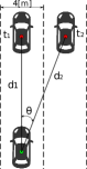
(a)

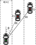
(b)

Figure 1: Considered automotive scenarios. Green circle: radar transmitter/receiver. Red circles: possible targets. Scenario (a) ($S_{(a)}$): two targets with similar ranges but different angles. Scenario (b) ($S_{(b)}$): two targets with similar angle but different ranges. The line width of a typical highway has been set to $4$ m. Other parameters are listed in Table I.

TABLE I: System parameters

$N=50$	$M=64$
$f_{c}=60$ [GHz]	$B=150$ [MHz]
$v_{\mathrm{res}}\simeq 421$ [km/h]	$r_{\mathrm{res}}\simeq 1$ [m]
$v_{\mathrm{max}}=N\cdot v_{\mathrm{res}}$	$r_{\mathrm{max}}=M\cdot r_{\mathrm{res}}$

Scheme	$d_{1}$ [m]	$d_{2}$ [m]	$v_{1}$ [km/h]	$v_{2}$ [km/h]	$\theta_{1}^{\circ}$	$\theta_{2}^{\circ}$
$S_{(a)}$	20	20.1	80.2	82.5	0.3	6.31
$S_{(b)}$	20.1	40.2	78.4	85.5	7.2	8.0

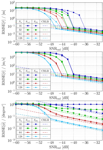
Figure 2: RMSE performance of Scheme (a) ($S_{(a)}$) and Scheme (b) ($S_{(b)}$) of Fig. 1 with a different number of antennas $N_{a}$.

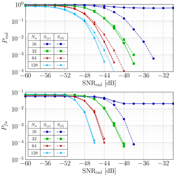
Figure 3: Miss detection $P_{md}$ and false alarm $P_{fa}$ probabilities of Scheme (a) ($S_{(a)}$) and Scheme (b) ($S_{(b)}$) of Fig. 1 with a different number of antennas $N_{a}$.

In order to cope with some illustrative automotive scenarios, we consider scenarios (a) and (b) of Fig. 1, while hybrid scenarios, as a combination of (a) and (b), can be a straightforward extension. Although (a) and (b) are LoS scenarios to ensure reliable communication at mmWave frequency bands (as in our simulations), the proposed algorithm can be applied to any other scenario and setup including the cases when multiple targets have exactly the same angle (e.g., at lower frequencies). Table I provides the system parameters, together with the parameters of the different analyzed scenarios. We define the radar SNR, from the backscattered signal, as [6, Chapter 2]

$$\mathrm{SNR_{rad}}=\frac{\lambda^{2}\sigma_{\mathrm{rcs}}G^{2}}{\left(4\pi\right)^{3}r^{4}}\frac{P_{\rm avg}}{\sigma_{w}^{2}}\,,$$ (25)

where $\lambda=c/f_{c}$ is the wavelength, $c$ is the speed of light, $\sigma_{\mathrm{rcs}}$ is the radar cross-section of the target in $\mathrm{m}^{2}$ ($\sigma_{\mathrm{rcs}}=1$ in our setup), $G$ is the antenna gain ($G=1$ in our setup), $r$ is the distance between transmitter and receiver, and $\sigma_{w}^{2}$ is the variance of the AWGN noise. In the case of multiple targets with different ranges, we set $\mathrm{SNR_{rad}}$ as the SNR of the nearest target.

While two distinct targets in the angle domain can be identified if the angular resolution meets some conditions (depending on the number of antennas, the angular distance between the two targets, and the array properties), a different analysis has to be done for Doppler and delay. In brief, given the parameters defined in Sec. II, velocity and range resolutions are

$$v_{\mathrm{res}}=\frac{Bc}{2NMf_{c}}\ \mathrm{[m/s]}\,,\>\>\>r_{\mathrm{res}}=\frac{c}{2B}\ \mathrm{[m]}\,.$$ (26)

In order to get a reasonable range resolution, e.g., $<1$ [m], a large bandwidth has to be considered. Since the velocity resolution is directly proportional to $B$, for a fixed $f_{c}$, the only way to obtain a fine resolution is to increase the block size $NM$, leading to a remarkable increase in computational complexity, which could be not affordable. For this reason, given the fact that multiple targets can be detected if separable in at least one domain out of three (angle, Doppler, delay), we fix the system parameters by focusing on a reasonable range resolution (and maximum range) under a feasible computational complexity. This in turn leads to an unavoidable very large velocity resolution. Clearly, under the system parameters of Table I, multiple targets are not separable solely in the Doppler domain.

Remark 3.

The performance of the proposed ML-based algorithm strictly depends on the dimension of the block of data sent, i.e., the product $N\cdot M$. Thus, the system parameters of Tab. I can be easily tuned to achieve the desired levels of radar resolutions (modifying the bandwidth), acquisition time (based on the length of the OTFS frame in time), maximum range, etc. Clearly, the CRLB changes accordly. Moreover, note that this is also possible thanks to OTFS modulation, which is not sensitive to Doppler and delay effects.

Fig. 2 shows the performance in terms of root MSE (RMSE) when an angular sector of $30$ degrees (from $-15^{\circ}$ to $15^{\circ}$) is covered (through an appropriate definition of the BF vector ${\bf f}_{\mathrm{BF}}$) for both scenarios (a) ($S_{(a)}$) and (b) ($S_{(b)}$) of Fig. 1, with parameters listed in Tab. I. Note that the RMSE is computed given the detection of the target within the angular sector. However, even if a target is correctly detected, if the SNR is not high enough, the parameter estimation performance might be not satisfactory. The probabilities of miss detection and false alarm, denoted by $P_{md}$ and $P_{fa}$, are provided in Fig. 3. The miss detection occurs when the presence of a target is not detected, i.e., the backscattered power is below the threshold, while the false alarm occurs when the received power in an angular sector is higher than the threshold, but no target is present.

In Fig. 2, we notice that after the “waterfall” transition, typical of ML estimators, all estimators achieve the respective CRLB up to a small-to-negligible loss due to the discretization error of the search over the three domains. In scenario (a), the algorithm is not able to distinguish two targets closed each other in the angle domain with $N_{a}=16$ antennas as observed in Fig. 3. This results in very poor angle estimation as seen in Fig. 2. This behavior does not occur in scenario (b), even with $N_{a}=16$, as two targets are well separated in the range domain. With $N_{a}=32$ antennas, the algorithm is able to distinguish two targets in scenario (a), as seen in Fig. 3, but cannot still achieve the desired angle estimation performance. Overall, the increase of the number of antennas leads to better asymptotic RMSE performance (lower CRLB) and detection probabilities, together with the capability of identifying nearest targets in the angle domain and reach the CRLB in any scenario.

Moreover, note that the heuristic definition of the detection threshold in Sec. III provides reasonable performance. In fact, beyond threshold SNR values at which the RMSE curves reach the corresponding CRLB, both probabilities of miss detection and false alarm achieve remarkable performance. Note that it is meaningful to operate at SNR values much higher than the “waterfall” behavior so that desired parameter estimation can be achieved.

V Conclusion

We studied the joint target detection and parameter estimation in a simple setup where a transmitter equipped with mono-static MIMO radar wishes to detect multiple targets and estimate the corresponding parameters using OTFS modulation and wide sector beams. We proposed an efficient ML-based approach that achieves good tradeoff between detection and estimation performance and complexity. Simulation results show that multiple targets are well identified if separable in at least one domain out of three (delay, Doppler, or angle), while achieving a small-to-negligible loss in terms of estimation error of typical radar parameters compared to CRLB. Moreover, the proposed algorithm is fully independent on the system setup and not restricted to any particular scenario.

References

- [1] J. Li and P. Stoica, MIMO radar signal processing. John Wiley & Sons, 2008.
- [2] S. M. Patole, M. Torlak, D. Wang, and M. Ali, “Automotive radars: A review of signal processing techniques,” IEEE Signal Process. Mag., vol. 34, no. 2, pp. 22–35, March 2017.
- [3] X. Song, S. Haghighatshoar, and G. Caire, “A scalable and statistically robust beam alignment technique for millimeter-wave systems,” IEEE Trans. Wireless Commun., vol. 17, no. 7, pp. 4792–4805, 2018.
- [4] B. Friedlander, “On transmit beamforming for MIMO radar,” IEEE Trans. Aerosp. Electron. Syst., vol. 48, no. 4, pp. 3376–3388, 2012.
- [5] U. Niesen and J. Unnikrishnan, “Joint beamforming and association design for MIMO radar,” IEEE Trans. Signal Process., vol. 67, no. 14, pp. 3663–3675, 2019.
- [6] M. A. Richards, Fundamentals of radar signal processing, Second edition. McGraw-Hill Education, 2014.
- [7] Y. Bar-Shalom and X.-R. Li, Multitarget-multisensor tracking: principles and techniques. YBs Storrs, CT, 1995, vol. 19.
- [8] L. Gaudio, M. Kobayashi, G. Caire, and G. Colavolpe, “On the effectiveness of OTFS for joint radar and communication,” arXiv preprint arXiv:1910.01896, 2019.
- [9] R. Hadani, S. Rakib, M. Tsatsanis, A. Monk, A. J. Goldsmith, A. F. Molisch, and R. Calderbank, “Orthogonal time frequency space modulation,” in 2017 IEEE Wireless Commun. and Network. Conf. (WCNC). IEEE, 2017, pp. 1–6.
- [10] S. H. Dokhanchi, B. S. Mysore, K. V. Mishra, and B. Ottersten, “A mmWave automotive joint radar-communications system,” IEEE Trans. Aerosp. Electron. Syst., vol. 55, no. 3, pp. 1241–1260, June 2019.
- [11] L. Zheng, M. Lops, Y. C. Eldar, and X. Wang, “Radar and communication co-existence: an overview: a review of recent methods,” IEEE Signal Process. Mag., vol. 36, no. 5, pp. 85–99, Sep. 2019.
- [12] A. Hassanien, M. G. Amin, E. Aboutanios, and B. Himed, “Dual-function radar communication systems: A solution to the spectrum congestion problem,” IEEE Signal Process. Mag., vol. 36, no. 5, pp. 115–126, Sep. 2019.
- [13] P. Raviteja, K. T. Phan, Y. Hong, and E. Viterbo, “Orthogonal time frequency space (OTFS) modulation based radar system,” in 2019 IEEE Radar Conf. (RadarConf). IEEE, 2019, pp. 1–6.
- [14] A. Sabharwal, P. Schniter, D. Guo, D. W. Bliss, S. Rangarajan, and R. Wichman, “In-band full-duplex wireless: Challenges and opportunities,” IEEE J. Sel. Areas Commun., vol. 32, no. 9, pp. 1637–1652, Sep. 2014.
- [15] X. Song, T. Kühne, and G. Caire, “Fully-/partially-connected hybrid beamforming architectures for mmWave MU-MIMO,” IEEE Trans. Wireless Commun., vol. 19, no. 3, pp. 1754–1769, 2020.
- [16] P. Kumari, J. Choi, N. González-Prelcic, and R. W. Heath, “IEEE 802.11ad-based radar: An approach to joint vehicular communication-radar system,” IEEE Trans. Veh. Technol., vol. 67, no. 4, pp. 3012–3027, April 2018.
- [17] D. H. N. Nguyen and R. W. Heath, “Delay and Doppler processing for multi-target detection with IEEE 802.11 OFDM signaling,” in Proc. IEEE Int. Conf. Acoustics, Speech, and Signal Processing (ICASSP), March 2017, pp. 3414–3418.
- [18] G. A. Vitetta, D. P. Taylor, G. Colavolpe, F. Pancaldi, and P. A. Martin, Wireless communications: algorithmic techniques. John Wiley & Sons, 2013.
- [19] S. Fortunati, L. Sanguinetti, F. Gini, M. S. Greco, and B. Himed, “Massive MIMO radar for target detection,” IEEE Trans. Signal Process., vol. 68, pp. 859–871, 2020.
- [20] G. Matz, H. Bolcskei, and F. Hlawatsch, “Time-frequency foundations of communications: Concepts and tools,” IEEE Signal Process. Mag., vol. 30, no. 6, pp. 87–96, Nov 2013.