Self-interacting neutrinos: solution to Hubble tension versus experimental constraints

Abstract

Exotic self-interactions among the Standard-Model neutrinos have been proposed as a potential reason behind the tension in the expansion rate, $H_{0}$, of the universe inferred from different observations. We constrain this proposal using electroweak precision observables, rare meson decays, and neutrinoless double-$\beta$ decay. In contrast to previous works, we emphasize the importance of carrying out this study in a framework with full Standard-Model gauge invariance. We implement this first by working with a relevant set of Standard-Model-Effective-Field-Theory operators and subsequently by considering a UV completion in the inverse See-Saw model. We find that the scenario in which all flavors of neutrinos self-interact universally is strongly constrained, disfavoring a potential solution to the $H_{0}$ problem in this case. The scenario with self-interactions only among tau neutrinos is the least constrained and can potentially be consistent with a solution to the $H_{0}$ problem.

I Introduction

There is a tantalizing discrepancy between the value of the Hubble constant ($H_{0}$) extracted from local measurement versus the one extracted from the Cosmic Microwave Background data Aghanim et al. (2018); Riess et al. (2018); Shanks et al. (2018); Riess et al. (2019); Wong et al. (2019).

Towards this end, the authors of Ref. Kreisch et al. (2019) suggested to give neutrinos a new, extra strong self-coupling in the form of the dimension-six operator

$$\mathscr{L}_{\text{eff}}\sim G_{\nu}(\bar{\nu}_{M}\nu_{M})(\bar{\nu}_{M}\nu_{M})\,.$$ (1)

We focus on the possibility that the Standard-Model (SM) neutrinos are Majorana, i.e., $\nu_{M}$ are four-component Majonara fermion fields. The Dirac case is strongly disfavoured by Big-Bang-Nucleosynthesis (BBN) constraints Blinov et al. (2019). This effective interaction can be induced by the presence of a light scalar mediator — a massive version of the so-called MajoronGelmini and Roncadelli (1981) — with an effective coupling

$$\mathscr{L}_{\text{eff Majoron}}\sim\lambda\phi\bar{\nu}_{M}\nu_{M}\,.$$ (2)

The effect of neutrino self-interactions in cosmological observables has been investigated in Refs. Oldengott et al. (2017); Lancaster et al. (2017); Archidiacono and Hannestad (2014); Cyr-Racine and Sigurdson (2014); Huang et al. (2018). The interaction in Eq. (1) can postpone the time at which the neutrinos begin to free stream and induce a phase shift towards high-$l$ scale at the CMB TT spectrum. Together with one additional sterile neutrino, which brings $N_{\text{eff}}\simeq 4$, this can reduce the tension in $H_{0}$. The fit of the CMB data favours two values for $G_{\nu}$, namely, SI$\nu$ (Strongly Interacting) and MI$\nu$ (Moderately Interacting)

$$G_{\nu}=\begin{cases}(4.6(5)~{}\text{MeV})^{-2}&(\text{SI}\nu)\\ (90^{+170}_{-60}~{}\text{MeV})^{-2}&(\text{MI}\nu)\end{cases}\,.$$ (3)

There have been many studies on the constraints of the neutrino–Majoron coupling. Experimental results like Supernova Farzan (2003); Kachelriess et al. (2000), neutrinoless double-$\beta$ decay Gando et al. (2012); Arnold et al. (2018), Meson decays Britton et al. (1994); Lazzeroni et al. (2013, 2011); Lessa and Peres (2007); Bakhti and Farzan (2017); Brdar et al. (2020) and $Z$-pole observables Abbiendi et al. (2004); Brdar et al. (2020) all give relevant constraints, see Ref. Blinov et al. (2019) for a summary of various bounds in the strong self-coupling scenario. However, most of the studies focus on the effective neutrino–Majoron coupling in Eq. (2), which violates electroweak gauge invariance. This is perfectly fine as long as one focuses on the degrees of freedom well below the weak scale. On the other hand, we have established a very accurate description of the physics around the weak scale, known as the Standard Model (SM). There are precision measurements that will set relevant constraints on the scenario of self-interacting neutrinos. Indeed, many of the studies did implemented such constraints, e.g., $Z$ decays. It is now mandatory to go beyond the effective interaction in Eq. (2) and consider weak-scale UV completions. While our analysis here is motivated by the solution to the Hubble tension, the results are general constraints on the neutrino self-coupling, whether it would play a role in interpreting the CMB data or not.

In this work, we take two consecutive steps in this direction.

Firstly, we will remain (mostly) agnostic about the specifics of new physics and assume that, apart from the Majoron itself, it is somewhat heavier than the weak scale. Hence, we will parameterize their effect by dimension-five and six effective operators in the Standard Model Effective Theory (SMEFT). One such dimension-six operator contains the Majoron and induces neutrino self-interactions. However, in typical models that modify the neutrino sector and induce neutrinos masses the aforementioned operator is accompanied by additional ones, which do not contain the Majoron, and are typically generated in any UV completion. We will use experimental data to constrain the size of their Wilson coefficients.

Secondly, we will consider the possibility of UV completing this effective theory into renormalizable models by introducing new degrees of freedom. Neutrinos are embedded in ${\rm SU}(2)$ doublets, therefore, at the renormalizable level the neutrino–Majoron coupling can only be induced via the (mass) eigenstate mixing after electroweak symmetry breaking. There are two paradigms: mixing with a neutrino sector or with a scalar sector. The former is realized in the Type-I seesaw model while the latter in Type-II. In both cases, the mixing angle determines the strength of the neutrino–Majoron coupling. However, we will see that for Type-I, the mixing is proportional to the neutrino mass and is thus too suppressed to provide a sufficiently large mixing. Similarly for Type-II, the current bound on the triplet Yukawa coupling and the vev of the triplet scalar implies that it cannot provide a sufficiently large mixing eitherFileviez Perez et al. (2008); Cai et al. (2018). However, we will show that there exist extended seesaw models in which there is no direct connection between the mixing and the neutrino mass. One of them is the so-called inverse seesaw model, which we will consider in detail. We will match the model to the SMEFT operators, and use the constraints derived for them to set limits on the model parameters.

We will find that within a SM gauge invariant framework, the extent to which neutrino self-interactions may alleviate the $H_{0}$ inconsistency depends on the flavour structure of the self-couplings. The case in which all flavours interact with the same strength (universal) is too constrained from electron-sector observables to provide a solution. However, the case in which only tau-flavor neutrinos self-interact may still provide a solution due to the weaker constraints from particle-physics observations.

The rest of this paper is organized as follows: In section II, we describe the relevant SMEFT framework and match it to seesaw models. In section III, we present the predictions for the observables entering the analysis. In section IV we combine the observables and contrast them to the CMB fit and discuss the various regions of the parameter space. We conclude in section V.

II The framework

II.1 Neutrino self-interactions within the extended SMEFT

We begin with the assumption that, with the exception of the Majoron $\phi$, new physics is heavier than the electroweak scale. In this case, all beyond-the-SM effects can be parameterized by a set of non-renormalizable operators. In our case, we are interested in a small subset of operators that induce neutrino self-interactions and those that typically accompany them in UV-complete models. More specifically, the following set suffices to capture the main phenomenological aspects

$$\mathscr{L}_{\text{EFT}}=C^{f}_{\nu\nu}~{}(Q^{f}_{\nu\nu}+\text{h.c.})+C^{f}_{\phi}~{}\phi(Q^{f}_{\phi}+\text{h.c.})\\ +C^{f}_{ew}~{}(Q_{HL}^{(1),f}-Q_{HL}^{(3),f})\,.$$ (4)

$f$ denotes the neutrino flavor with $f=e,\mu,\tau$, and

$$\begin{split}Q^{f}_{\nu\nu}&=\overline{L^{c}}_{f}\tilde{H}^{*}\tilde{H}^{\dagger}L_{f}\\ Q^{f}_{\phi}&=\phi\overline{L^{c}}_{f}\tilde{H}^{*}\tilde{H}^{\dagger}L_{f}\\ Q_{HL}^{(1),f}&=(H^{\dagger}i\,\mbox{$\raisebox{5.69054pt}{${}^{\leftrightarrow}$}D_{\mu}$}H)(\overline{L}_{f}\gamma^{\mu}L_{f})\\ Q_{HL}^{(3),f}&=(H^{\dagger}i\,\mbox{$\raisebox{5.69054pt}{${}^{\leftrightarrow}$}D^{I}_{\mu}$}H)(\overline{L}_{f}\sigma^{I}\gamma^{\mu}L_{f})\,.\end{split}$$ (5)

Our notation follows closely the ones of Ref. Grzadkowski et al. (2010). We ignore flavor-changing operators and restrict the discussion to flavor-diagonal operators.

The SM neutrinos live in the weak doublets $L_{f}$, thus the Higgs doublet $H$ must be included to form gauge singlets. The dimension-five Weinberg operator, $Q^{f}_{\nu\nu}$, accounts for neutrino masses. The operator $Q^{f}_{\phi}$ is responsible for generating the self-interaction. The operators $Q_{HL}^{(1),f}$ and $Q_{HL}^{(3),f}$ must also be included, because they are typically also generated at the tree-level in models that induce $Q^{f}_{\nu\nu}$. In particular, the operators $Q_{HL}^{(1),f}$ and $Q_{HL}^{(3),f}$ are typically generated with a Wilson coefficient of same magnitude but opposite sign, i.e., $C_{HL}^{(1),f}=C_{ew}^{f}$ and $C_{HL}^{(3),f}=-C_{ew}^{f}$ (we have already implemented this in Eq. (4)). The reason behind this tree-level relation is that typical models that generate the $Q^{f}_{\nu\nu}$ operator by integrating out some heavy degrees of freedom, also necessarily induce the derivative operator $(\overline{L}_{f}\tilde{H})i\not{\partial}(\tilde{H}^{\dagger}L_{f})$. This derivative operator is redundant in the Warsaw basis, where it is removed in favor of the combination $Q_{HL}^{(1),f}-Q_{HL}^{(3),f}=4(\overline{L}_{f}\tilde{H})i\not{\partial}(\tilde{H}^{\dagger}L_{f})$. The presence of these operators lead to important phenomenological consequences, which cannot be captured when one simply works with the effective coupling in Eq. (2).

To work with dimensionless couplings for the dimension-six Wilson coefficients we introduce the notation $\bar{C}_{X}=C_{X}v^{2}$, with $v\simeq 246$ GeV the electroweak vev.

At scales below the electroweak scale the $Q^{f}_{\nu\nu}$ operators induce a Majorana mass term for the neutrinos, and the $Q^{f}_{\phi}$ couplings of the neutrinos to $\phi$. The resulting Lagrangian reads

$$\mathscr{L}_{\nu}=\frac{1}{2}\bar{\nu}_{M,f}(i\not{\partial}-m_{\nu_{f}})\nu_{M,f}+\frac{1}{2}\lambda_{f}\phi\bar{\nu}_{M,f}\nu_{M,f}$$ (6)

with $\nu_{M,f}=\nu_{L,f}+(\nu_{L,f})^{c}$ the four-component Majorana fermion and where

$$m_{\nu_{f}}=-\bar{C}^{f}_{\nu\nu}\,, \lambda_{f}=\bar{C}^{f}_{\phi}\,.$$ (7)

We note that both the mass and the interaction in Eq. 6 are flavor diagonal. We emphasize that this is an assumption, and more general flavor structures are certainly possible. However, the aim of this work is to extract main lessons rather than carry out an exhaustive study. Moreover, as we will see in section III.4, the effect of neutrino self-interactions on the CMB has only been studied under a quite (over)simplified case. Hence, we will also make simplifying assumptions for the flavor structure in our study.

II.2 Seesaw Models

II.2.1 Type-I Seesaw Model

To illustrate how the EFT operators presented in section II.1 are induced in concrete UV models we start with the simplest Type-I seesaw model. The SM Lagrangian is augmented with an extra heavy right-handed neutrino

$$\mathscr{L}\supset\overline{N_{R}}i\not{\partial}N_{R}-\dfrac{M_{R}}{2}(\overline{N_{R}^{c}}N_{R}+\overline{N_{R}}N_{R}^{c})\\ +(-y_{R}\bar{L}\tilde{H}N_{R}+\dfrac{1}{2}\lambda\phi\overline{N_{R}^{c}}N_{R}+\text{h.c.})\,.$$ (8)

with $N_{R}$ a four-component chiral field. After electroweak symmetry breaking, the mixed Dirac mass is generated $m_{D}=y_{R}v/\sqrt{2}$. The neutrino mass matrix then reads

$$M=\begin{pmatrix}0&m_{D}\\ m_{D}&M_{R}\end{pmatrix}\,.$$ (9)

After diagonalization, the masses of the light mass eigenstates in the limit $m_{D}\ll M_{R}$ are

$$m_{\nu}=\frac{m_{D}^{2}}{M_{R}}\,,$$ (10)

and the mixing angle between light and heavy eigenstates is

$$\sin\theta\sim\dfrac{m_{D}}{M_{R}}\,.$$ (11)

Hence, the coupling between the Majoron and light eigenstates reads

$$g_{\phi\nu\nu}=\lambda\left(\dfrac{m_{D}}{M_{R}}\right)^{2}=\lambda\dfrac{m_{\nu}}{M_{R}}\,.$$ (12)

We see that in this model the coupling to the Majoron is suppressed by the neutrino mass and thus cannot produce strong self-interactions for perturbative values of $\lambda$.

To match to the effective Lagrangian in Eq. (4), we integrate out $N_{R}$ at the tree-level and find the Wilson coefficients

$$C^{f}_{\nu\nu}=-\frac{y_{R}^{2}}{2}\frac{1}{M_{R}}, C^{f}_{\phi}=\frac{\lambda}{2}\frac{y_{R}^{2}}{M_{R}^{2}}, C^{f}_{ew}=\frac{1}{4}\frac{y_{R}^{2}}{M_{R}^{2}}.$$ (13)

Again, we see that $C^{f}_{\nu\nu}$, which generates the neutrino mass, is correlated to $C^{f}_{\phi}$. Hence, the neutrino–Majoron interaction, proportional to $C^{f}_{\phi}$, is suppressed by the neutrino mass.

II.2.2 Inverse Seesaw Model

In order to break the correlation between $C^{f}_{\nu\nu}$ and $C^{f}_{\phi}$ we consider an inverse seesaw model Dias et al. (2012); Law and McDonald (2013); Mohapatra and Valle (1986); Ma (1987, 2009); Bazzocchi (2011) augmented with an additional real scalar, $\phi$, that couples to one species of the heavy neutrinos:

$$\mathscr{L}_{\text{inv-seesaw}} =i\overline{\mathcal{F}}\not{\partial}\mathcal{F}-M\overline{\mathcal{F}}\mathcal{F}$$

$$-\left(\frac{\delta_{R}}{2}\overline{\mathcal{F}_{R}^{c}}F_{R}+\frac{\delta_{L}}{2}\overline{\mathcal{F}_{L}^{c}}F_{L}+y_{R,f}\overline{L}_{f}\tilde{H}\mathcal{F}_{R}+\text{h.c.}\right)$$

$$+\frac{\lambda}{2}\phi\left(\overline{\mathcal{F}_{L}^{c}}F_{L}+\text{h.c.}\right)\,,$$ (14)

with $\mathcal{F}=\mathcal{F}_{L}+\mathcal{F}_{R}$. The fermion fields $\mathcal{F}_{L}$ and $\mathcal{F}_{R}$ above are four-component chiral fields, i.e., only two components are non-zero. By choosing to couple the Majoron only to $\mathcal{F}_{L}$ and not to $\mathcal{F}_{R}$ we break the correlation between neutrino mass and Majoron coupling. The subscript, $f$, stands for the flavor. For simplicity we consider the heavy-neutrino setting for each flavor separately and do not consider their mixing.

We match to the effective Lagrangian in Eq. (4) by integrating out the heavy fields $\mathcal{F}_{R}$ and $\mathcal{F}_{L}$ at the tree-level. For the case $\delta_{L},\,\delta_{R}\ll M$ and up to dimension-six the Wilson coefficients we obtain are

$$C^{f}_{\nu\nu}=-\frac{y_{R,f}^{2}}{2}\frac{\delta_{L}}{M^{2}}\,, C^{f}_{\phi}=\frac{\lambda}{2}\frac{y_{R,f}^{2}}{M^{2}}\,, C^{f}_{ew}=\frac{1}{4}\frac{y_{R,f}^{2}}{M^{2}}\,.$$ (15)

Contrary to the Type-I model, we see that the neutrino mass and the neutrino–Majoron coupling are controlled by independent parameters, $\delta_{L}$ and $\lambda$, respectively.

It is thus possible to induce a sizable neutrino–Majoron coupling without it being suppressed by the neutrino mass. At the same time, we see that $C^{f}_{\phi}$ and $C^{f}_{ew}$ are correlated to some extent, which has important phenomenological consequences.

To include constraints from electroweak-precision observables, we also compute the Wilson coefficient of the operator that contributes to the $T$-parameter at tree level. In the Warsaw basis this operator is $Q_{HD}\equiv|H^{\dagger}D^{\mu}H|^{2}$. The one-loop matching at a scale $\mu\simeq M$ gives

$$L\supset C_{HD}Q_{HD}\quad\text{with}\quad C_{HD}(M)=-\frac{1}{16\pi^{2}}\frac{y_{R,f}^{4}}{2M^{2}}\,,$$ (16)

where we only kept terms of ${\cal O}(y_{R,f}^{4})$. We include the leading terms of ${\cal O}(y_{R,f}^{2}g_{1}^{2},y_{R,f}^{2}y_{e}^{2})$ by solving the renormalization group (RG) within SMEFT (see section III.2).

III Observables

In this section we discuss the most relevant observables in our analysis and their predictions within the SMEFT framework. We choose as the numerical input for the electroweak parameters $G_{F}$, $\alpha$, and $m_{Z}$. As extensively discussed in the literature, e.g., Ref. Brivio et al. (2017) and references within, the presence of dimension-six operators affects the determination of the electroweak-parameter input. In the case at hand, only the operators in Eq. (5) are induced at the tree-level and in fact out of them only the operators $Q_{HL}^{(3),e}$ and $Q_{HL}^{(3),\mu}$ affect the extraction of $G_{F}$. The remaining electroweak input remains unchanged. The $G_{F}$ shift affects all electroweak observables. To take it into account, one substitutes, e.g., Ref. Brivio et al. (2017),

$$G_{F}\longrightarrow G_{F}\left(1-\bar{C}_{HL}^{(3),e}-\bar{C}_{HL}^{(3),\mu}\right)=\\ =G_{F}\left(1+\bar{C}_{ew}^{e}+\bar{C}_{ew}^{\mu}\right)\,,$$ (17)

where $G_{F}$ is still the experimental input value.

III.1 $Z$ decays

After electroweak-symmetry breaking the operator combination $Q^{(1),f}_{HL}-Q^{(3),f}_{HL}$ does not (directly) affect the charged lepton sector, but it does induce an anomalous $Z$ coupling to the neutrino species $f$, i.e.,

$$\mathscr{L}_{\text{anom-}Z}=-\frac{e}{2s_{w}c_{w}}2\bar{C}^{f}_{ew}\bar{\nu}^{f}_{L}\not{Z}\nu^{f}_{L}\,.$$ (18)

Together with the shift in $G_{F}$ this modifies the partial width to the neutrinos

$$\Gamma(Z\to\bar{\nu}_{f}\nu_{f})=\frac{G_{F}m_{Z}^{3}}{12\sqrt{2}\pi}(1+\bar{C}^{e}_{ew}+\bar{C}^{\mu}_{ew}-4\bar{C}^{f}_{ew})\,.$$ (19)

We also include the three-body partial width $Z\to\bar{\nu}_{f}\nu_{f}\phi$, which is, however, formally higher order in the EFT, i.e., it is proportional to $(\bar{C}^{f}_{\phi})^{2}$. For the region of interest $m_{\phi}\ll m_{Z}$, we find for a neutrino species coupled to $\phi$ via the operator $Q^{f}_{\phi}$ the width

$$\Gamma(Z\to\bar{\nu}_{f}\nu_{f}\phi)=\frac{G_{F}m_{Z}^{3}}{12\sqrt{2}\pi}\frac{(\bar{C}^{f}_{\phi})^{2}}{192\pi^{2}}\left(12\log\biggl{(}\dfrac{m_{Z}^{2}}{m_{\phi}^{2}}\biggr{)}-23\right)\,.$$ (20)

Notice that this rate diverges for $m_{\phi}\to 0$. For small $m_{\phi}$ it is thus necessary to resum the logarithms. However, for the masses that we are considering this is not necessary. Also due to the double EFT suppression this rate is numerically small.

Similarly we evaluate the effect of the shift in $G_{F}$ in the partial width to charged leptons and to hadrons. In the SM the partial width to a fermion $f$ with charge $Q^{f}$ is

$$\Gamma(Z\to\bar{f}f)^{\text{SM}}=n_{c}^{f}\frac{\alpha m_{Z}}{24s_{w}^{2}c_{w}^{2}}\left(1-4s_{w}^{2}|Q^{f}|+8s_{w}^{4}|Q^{f}|^{2}\right)\,.$$ (21)

After shifting $G_{F}$ we find that

$$\Gamma(Z\to\ell^{+}\ell^{-})=\Gamma(Z\to\ell^{+}\ell^{-})^{\text{SM}}\times\\ \times\left(1+(\bar{C}_{ew}^{e}+\bar{C}_{ew}^{\mu})\frac{1-2s_{w}^{2}-4s_{w}^{4}}{(1-2s_{w}^{2})(1-4s_{w}^{2}+8s_{w}^{4})}\right)\,,$$ (22)

$$\Gamma(Z\to\text{hadrons})=\Gamma(Z\to\text{hadrons})^{\text{SM}}\times\\ \times\left(1+(\bar{C}_{ew}^{e}+\bar{C}_{ew}^{\mu})\frac{45-90s_{w}^{2}-4s_{w}^{4}}{(1-2s_{w}^{2})(45-84s_{w}^{2}+88s_{w}^{4})}\right)\,.$$ (23)

III.2 $T$-parameter

Heavy sterile neutrinos can affect electroweak-precision observables, i.e., the $T$-parameter. Within the SMEFT framework the new-physics contributions to the $T$-parameter are controlled by the Wilson coefficient of the $Q_{HD}$ operator evaluated at the electroweak scale, $\mu_{\text{ew}}\sim m_{Z}$, via $\alpha T=\hat{T}=-\frac{v^{2}}{2}C_{HD}(\mu_{\text{ew}})$ Barbieri et al. (2004). In our setup we integrate out the heavy degrees of freedom at a scale $M\gg\mu_{\text{ew}}$ and obtain $C_{HD}(\mu_{\text{ew}})$ via the RG evolution to $\mu_{\text{ew}}$ (see Refs. Alonso et al. (2014); Jenkins et al. (2014) for the corresponding anomalous dimensions). Operators that have been induced at the tree-level at $M$ can mix into $Q_{HD}$. In our case we find that at leading-log accuracy

$$C_{HD}(m_{Z}) =C_{HD}(M)$$ (24)

$$-\frac{e^{2}}{16\pi^{2}}\left(\frac{8}{3c_{w}^{2}}+\frac{4}{s_{w}^{2}c_{w}^{2}}\frac{m_{f}^{2}}{m_{Z}^{2}}\right)C^{(1),f}_{HL}\log\frac{m_{Z}}{M}\,.$$

The singlet operators $Q_{HL}^{(1),f}$ mix into $Q_{HD}$, introducing the dependence on $C^{(1),f}_{HL}=C_{ew}^{f}$.

III.3 Leptonic meson decays

Non-standard neutrino interactions affect the decays of pseudoscalar mesons. The most stringent constraints originate from the semileptonic decays of charged pseudoscalars. The modification with respect to the SM originates both from the shift in $G_{F}$ and the anomalous coupling $W\ell_{f}\nu_{f}$ proportional to $\frac{e}{\sqrt{2}s_{w}}\bar{C}^{(3),f}_{HL}$. The two-body partial width of a pseudoscalar, $P$, to a neutrino and a charged lepton then reads

$$\Gamma(P\rightarrow\ell_{f}\nu_{f})=\dfrac{G_{F}^{2}}{8\pi}f_{P}^{2}m_{\ell_{f}}^{2}m_{P}\Big{(}1-\dfrac{m_{\ell_{f}}^{2}}{m_{P}^{2}}\Big{)}V_{\text{CKM}}\times\\ \times\left(1+2\big{(}\bar{C}^{e}_{ew}+\bar{C}^{\mu}_{ew}-\bar{C}^{f}_{ew}\big{)}\right)\,,$$ (25)

with $f_{P}$ the decay constant of the meson and $V_{\text{CKM}}=|V_{u_{i}d_{j}}|^{2}$ the corresponding CKM elements. As in the SM the two-body widths are helicity suppressed and thus proportional to the charged lepton mass.

The helicity suppression is lifted in the three-body decay $P\rightarrow\ell_{f}\nu_{f}\phi$. Expanding in the mass of the charged lepton we find

$$\Gamma(P\rightarrow\ell_{f}\nu_{f}\phi)=\dfrac{f_{P}^{2}G_{F}^{2}V_{\text{CKM}}m_{P}^{3}}{768\pi^{3}}({\bar{C}}_{\phi}^{f})^{2}\times\\ \times\left(1+9x_{\phi}-9x_{\phi}^{2}-x_{\phi}^{3}+6(x_{\phi}+1)x_{\phi}\log x_{\phi}\right)\,,$$ (26)

where $x_{\phi}=m_{\phi}^{2}/m_{P}^{2}$.

III.4 Neutrino self-scattering ($G_{\nu}$)

The presence of new, neutrino self-interactions can modify the neutrino standard free-streaming behavior during the radiation-dominated era. $2\to 2$ scattering among neutrinos modifies the momentum dependence of the neutrino distribution functions and can thus affect cosmological observables such as the CMB. The cosmological fit of Ref. Kreisch et al. (2019) is performed for the case in which the $\phi$ mass is much larger than the typical energy scale of the scattering event. In this case we can to an excellent approximation integrate out $\phi$ and describe the neutrino self-interactions via four-fermion contact interactions.

Starting from the (per assumption) flavor-diagonal Lagrangian for the four-component Majorana fermions $\nu_{M,i}$ in Eq. (6) we use the EOM of the real scalar ($(\Box+m_{\phi}^{2})\phi=\frac{1}{2}\sum_{i}\bar{C}_{\phi}^{i}\bar{\nu}_{M,i}\nu_{M,i}$) to obtain the effective Lagrangian

$$\begin{split}\mathscr{L}_{\nu,\text{eff}}&=\frac{1}{8m_{\phi}^{2}}\sum_{i,j}\bar{C}_{\phi}^{i}\bar{C}_{\phi}^{j}(\bar{\nu}_{M,i}\nu_{M,i})(\bar{\nu}_{M,j}\nu_{M,j})\\ &=\frac{1}{8}\sum_{i=1,2,3}C_{\nu\nu}^{i}(\bar{\nu}_{M,i}\nu_{M,i})(\bar{\nu}_{M,i}\nu_{M,i})\\ &+\frac{1}{4}\sum_{\begin{subarray}{c}i,j=1,2,3\\ i<j\end{subarray}}C_{\nu\nu}^{ij}(\bar{\nu}_{M,i}\nu_{M,i})(\bar{\nu}_{M,j}\nu_{M,j})\end{split}$$ (27)

with

$$C_{\nu\nu}^{i}=\frac{(\bar{C}_{\phi}^{i})^{2}}{m_{\phi}^{2}}\,, C_{\nu\nu}^{ij}=\frac{\bar{C}_{\phi}^{i}\bar{C}_{\phi}^{j}}{m_{\phi}^{2}}\quad\text{with}~{}i<j\,.$$ (28)

Here, the indices $i,j=1,2,3$ indicate the flavors $e,\mu,\tau$, respectively. Note that when $\phi$ couples flavour-diagonally to more that one flavour a mixed four-fermion operator is necessarily generated.

In order to make contact with the results of the CMB fit of Ref. Kreisch et al. (2019) we present here the corresponding collision terms for neutrino scattering. In the general, flavour-diagonal case there are three independent processes: the self-scattering of one species ($\nu_{i}+\nu_{i}\to\nu_{i}+\nu_{i}$), $s$-channel annihilation ($\nu_{i}+\nu_{i}\to\nu_{j}+\nu_{j}$ with $i\neq j$), and $t$-channel scattering ($\nu_{i}+\nu_{j}\to\nu_{i}+\nu_{j}$ with $i\neq j$). Their respective squared matrix-elements summed over initial- and final-state spins are:

$$|{\cal M}^{i}_{s,t,u}|^{2} \equiv\sum_{\text{spins}}|{\cal M}_{\nu_{i}\nu_{i}\to\nu_{i}\nu_{i}}|^{2}$$

$$=2(C_{\nu\nu}^{i})^{2}\left(s^{2}+t^{2}+u^{2}\right)$$

$$=2\frac{(\bar{C}_{\phi}^{i})^{4}}{m_{\phi}^{4}}\left(s^{2}+t^{2}+u^{2}\right)\,,$$ (29)

$$|{\cal M}^{ij}_{s}|^{2} \equiv\sum_{\text{spins}}|{\cal M}_{\nu_{i}\nu_{i}\to\nu_{j}\nu_{j}}|^{2}=4(C_{\nu\nu}^{ij})s^{2}$$

$$=4\frac{(\bar{C}_{\phi}^{i})^{2}(\bar{C}_{\phi}^{j})^{2}}{m_{\phi}^{4}})s^{2}\qquad\text{with}\quad i<j\,,$$ (30)

$$|{\cal M}^{ij}_{t}|^{2} \equiv\sum_{\text{spins}}|{\cal M}_{\nu_{i}\nu_{j}\to\nu_{i}\nu_{j}}|^{2}=4(C_{\nu\nu}^{ij})^{2}t^{2}$$

$$=4\frac{(\bar{C}_{\phi}^{i})^{2}(\bar{C}_{\phi}^{j})^{2}}{m_{\phi}^{4}})t^{2}\qquad\text{with}\quad i<j\,,$$ (31)

with $s,t,u$ the usual Mandelstam variables. No symmetry factors for identical particles have been included above.

What enters the evolution of the neutrino distributions are the collision integrals for each process. Adapting the generic expression from Ref. Kolb and Turner (1990) we find that for a specific neutrino species $i$ and $j\neq i$ the collision integrals for the three processes above are:

$$\mathscr{C}_{\nu_{i}(p_{1})\nu_{i}(p_{2})\leftrightarrow\nu_{i}(p_{3})\nu_{i}(p_{4})}=\frac{1}{2g}\int d\Pi_{2}d\Pi_{3}d\Pi_{4}~{}(2\pi)^{4}\times\\ \times F[\nu_{i}(p_{1}),\nu_{i}(p_{2});\nu_{i}(p_{3}),\nu_{i}(p_{4})]\times\\ \times\delta(p_{1}+p_{2}-p_{3}-p_{4})~{}|{\cal M}^{i}_{s,t,u}|^{2}\,,$$ (32)

$$\mathscr{C}_{\nu_{i}(p_{1})\nu_{i}(p_{2})\leftrightarrow\nu_{j}(p_{3})\nu_{j}(p_{4})}=\frac{1}{2g}\int d\Pi_{2}d\Pi_{3}d\Pi_{4}~{}(2\pi)^{4}\times\\ \times F[\nu_{i}(p_{1}),\nu_{i}(p_{2});\nu_{j}(p_{3}),\nu_{j}(p_{4})]\times\\ \times\delta(p_{1}+p_{2}-p_{3}-p_{4})~{}\frac{1}{2}|{\cal M}^{ij}_{s}|^{2}\,,$$ (33)

$$\mathscr{C}_{\nu_{i}(p_{1})\nu_{j}(p_{2})\leftrightarrow\nu_{i}(p_{3})\nu_{j}(p_{4})}=\frac{1}{2g}\int d\Pi_{2}d\Pi_{3}d\Pi_{4}~{}(2\pi)^{4}\times\\ \times F[\nu_{i}(p_{1}),\nu_{j}(p_{2});\nu_{i}(p_{3}),\nu_{j}(p_{4})]\times\\ \times\delta(p_{1}+p_{2}-p_{3}-p_{4})|{\cal M}^{ij}_{t}|^{2}\,,$$ (34)

where $d\Pi_{i}=\frac{d^{3}p_{i}}{(2\pi)^{3}2E_{i}}$ and $F[\dots]$ defined as in Ref. Kreisch et al. (2019). The factor $1/g$, with $g=2$ the spin degrees of freedom, has been omitted in Ref. Kreisch et al. (2019). No additional symmetry factors for identical particles in initial and final state need to be included in Eq. (32) (see Ref. Gondolo and Gelmini (1991)). The factor $1/2$ in Eq. (33) is due to the identical particles $j\neq i$ in the final or initial state.

We see that the collision integrals in Eqs. (33) and (34) couple the evolution of the distribution function of the three species. This cross-talk has been been neglected in Ref. Kreisch et al. (2019). Instead each neutrino flavour was assumed to self-interact independently with the same strength and the fit to the CMB provided the best-fit value for the parameter $G_{\nu}$ defined via the collision integral for each species Kreisch et al. (2019)

$$\mathscr{C}^{\text{Ref.~{}\cite[cite]{\@@bibref{Authors Phrase1YearPhrase2}{Kreisch:2019yzn}{\@@citephrase{(}}{\@@citephrase{)}}}}}_{\nu_{i}(p_{1})\nu_{i}(p_{2})\leftrightarrow\nu_{i}(p_{3})\nu_{i}(p_{4})}=\frac{1}{2}\int d\Pi_{2}d\Pi_{3}d\Pi_{4}~{}(2\pi)^{4}\times\\ \times F[\nu_{i}(p_{1}),\nu_{i}(p_{2});\nu_{i}(p_{3}),\nu_{i}(p_{4})]\\ \times\delta(p_{1}+p_{2}-p_{3}-p_{4})~{}2~{}G_{\nu}^{2}(s^{2}+t^{2}+u^{2})\,,$$ (35)

We emphasize again that this is an over-simplifying assumption that does not follow from flavor universality. Nevertheless, we will use it since it provides a direct comparison between the explicit fit performed in Ref. Kreisch et al. (2019) and the constraints obtained in this paper. Under this simplifying assumption, i.e., neglecting cross-talk, we find by comparing Eqs. (32) and (35) that for the “universal case” ($C_{\nu\nu}^{1}=C_{\nu\nu}^{2}=C_{\nu\nu}^{3}=C_{\nu\nu}^{12}=C_{\nu\nu}^{13}=C_{\nu\nu}^{23}\equiv C_{\nu\nu}$)

$$C_{\nu\nu}\longleftrightarrow\sqrt{2}G_{\nu}\,.$$ (36)

Additionally to the “universal” case, we also consider “flavor specific” cases (one $C^{i}_{\nu\nu}\neq 0$ and all other couplings zero) in which the self-interactions take place only among a single species instead of among all three. These cases are governed by the evolution of the thermal bath of one neutrino with the collision integral in Eq. (32). The fit of Ref. Kreisch et al. (2019) does not cover these cases, a dedicated re-analysis is required, which is beyond the scope of the present work. Roughly, the total strength of self-interactions are weaker if a single species self-interacts than in the “universal case”. To at least partially take this into account we interpret the fit of Ref. Kreisch et al. (2019) for the “flavor specific” case via the rescaling

$$C^{i}_{\nu\nu}\longleftrightarrow\sqrt{6}G_{\nu}\,.$$ (37)

The results of a future CMB fit for these cases could then be obtained by a simple rescaling of Eq. (37). We caution that while we expect this scaling to partially take into account the difference between the effective coupling strength, the factor of $\sqrt{6}$ is just an educated guess. More complete numerical study is needed to obtain the precise factor.

For the cases we consider, the two best-fit regions from Ref. Kreisch et al. (2019) in Eq. (3) then translate into:

$$v^{2}|C_{\phi}|=\frac{m_{\phi}}{\text{MeV}}~{}\times\begin{Bmatrix}(4.6(5))^{-1}&(\text{SI}\nu)\\ (90^{+170}_{-60})^{-1}&(\text{MI}\nu)\end{Bmatrix}\times\\ \times\begin{Bmatrix}2^{\frac{1}{4}}&(\text{``flavor-specific'' case})\\ 6^{\frac{1}{4}}&(\text{``universal'' case})\\ \end{Bmatrix}\,.$$ (38)

IV Numerical Analysis

As we have discussed above, we focus on two distinct limits in both of which the self-interactions via $\phi$ are assumed to be aligned to the neutrino mass-eigenstates.

“Flavor-specific” cases:

Self-interactions are present only for one, the $f$-th species of neutrinos with $f=e,\mu,\tau$. In this case $\bar{C}_{\phi}^{f}\,,\bar{C}_{ew}^{f}\neq 0$ while $\bar{C}_{\phi}^{f^{\prime}}=\bar{C}_{ew}^{f^{\prime}}=0$ for $f^{\prime}\neq f$.

“Universal” case:

All three neutrinos species interact with equal strength such that $\bar{C}_{\phi}\equiv\bar{C}_{\phi}^{e}=\bar{C}_{\phi}^{\mu}=\bar{C}_{\phi}^{\tau}$ and $\bar{C}_{ew}\equiv\bar{C}_{ew}^{e}=\bar{C}_{ew}^{\mu}=\bar{C}_{ew}^{\tau}$.

IV.1 Experimental input / Constraints

To illustrate the relative importance of various particle-physics and cosmological observables in the “flavor-specific” and “universal” cases we perform $\chi^{2}$ fits combining information from multiple observables. Below we summarize the experimental input relevant for the fits. Any additional, unspecified numerical input is taken from Ref. Tanabashi et al. (2018).

1. Z decays: We implement the constraints from the partial width measurements of the $Z$ boson by centering the corresponding $\chi^{2}$’s around the SM predictions and using the experimental uncertainties Tanabashi et al. (2018)

   $$\Delta\Gamma_{\ell^{+}\ell^{-}} =0.086\text{ MeV}\,,$$

   $$\Delta\Gamma_{\text{had}} =2.0\text{ MeV}\,,$$

   $$\Delta\Gamma_{\text{inv}} =1.5\text{ MeV}\,.$$

2. $T$-parameter: When discussing the inverse seesaw model we also include the constraint from the $T$-parameter as it can be affected by the presence of heavy neutrinos. We use the current best fit value of $T=0.06\pm 0.06$ Tanabashi et al. (2018).

3. Meson decays: Analogously to $Z$ decays also for meson decays we assume that the experimental measurements of their branching ratios and their lifetimes are centered around their SM predictions and add the corresponding experimental uncertainties in their $\chi^{2}$. We neglect subleading theory uncertainties associated to form-factors. We consider constraints from branchings fractions of two-body leptonic decays of $\pi^{+}$, $K^{+}$, $D_{s}^{+}$, as well as their lifetimes Tanabashi et al. (2018):

   $$\Delta\text{BR}(\pi^{+}\to e^{+}\nu,\mu^{+}\nu) =4\!\times\!10^{-7}\,,4\!\times\!10^{-7}$$

   $$\Delta\text{BR}(K^{+}\to e^{+}\nu,\mu^{+}\nu) =7\!\times\!10^{-8}\,,1.1\!\times\!10^{-3}\,,$$

   $$\Delta\text{BR}(D_{s}^{+}\to\mu^{+}\nu,\tau^{+}\nu) =2.3\!\times\!10^{-4}\,,2.3\!\times\!10^{-3}\,,$$

   $$\Delta\tau_{\pi^{+}} =5\!\times\!10^{-12}\,\text{sec}\,,$$

   $$\Delta\tau_{K^{+}} =2\!\times\!10^{-11}\,\text{sec}\,,$$

   $$\Delta\tau_{D_{s}^{+}} =4\!\times\!10^{-15}\,\text{sec}\,.$$

   Note that often measurement of ratios of branching fractions are more constraining than those from the branching ratios above. However, using such ratios can leave certain directions unconstrained when more than one neutrino species self-interact, i.e., in the “universal” case. The combination of constraints are, however, similar when folded with the lifetimes measurements and $Z$ decays. Therefore, to enable a better comparison between different cases we do not include ratios of branching ratios in the fits.

4. Neutrinoless double $\beta$-decay: As discussed in Ref. Blum et al. (2018), current neutrinoless double $\beta$-decay experiments like NEMO-3 Arnold et al. (2014) and KamLAND-Zen Gando et al. (2012) can stringently constrain light $e$-flavor Majorons. This will be illustrated by mapping the results of Figure 4 of Ref. Blum et al. (2018) into our corresponding exclusion plots.

5. BBN: Strong constraints are imposed on light species remaining in thermal equilibrium with neutrinos as extra relativistic degrees of freedom during the BBN period, as they affect the effective number of neutrinos, $\Delta N_{\text{eff}}$. Here, we follow the analysis of Ref. Blinov et al. (2019) and consider the mass of the real scalar to be above $1$ MeV.

IV.2 SMEFT fit

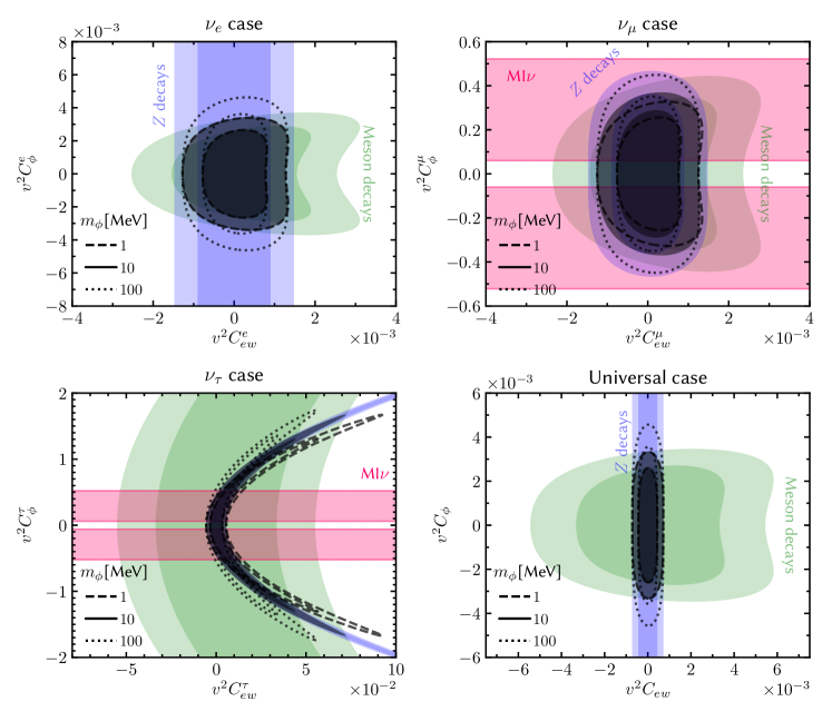
Figure 1: Preferred $68.27\%$ and $95.45\%$ CL regions for the Wilson coefficients $\bar{C}^{(i)}_{ew}$ and $\bar{C}_{\phi}^{(i)}$. Each panel corresponds to one of the four cases ($\nu_{e}$, $\nu_{\mu}$, $\nu_{\tau}$, and universal). In purple and green the constraints from $Z$ and leptonic meson decays, respectively. In black (gray) the combined allowed $68.27\%$ ($95.45\%$) CL region. The red regions in the second and third plot correspond to the $1\sigma$ preferred region for MI$\nu$ in Ref. Kreisch et al. (2019), cf., Eq. (38). The best-fit regions for the SI$\nu$ case and the MI$\nu$ case not appearing in the first and last plot lie outside the ranges. All coloured regions correspond to $m_{\phi}=10$ MeV. For the combined constraints we show the allowed region for $m_{\phi}=1$ MeV and $m_{\phi}=100$ MeV in dashed and dotted lines, respectively.

We first investigate the constraints on the SMEFT Wilson coefficients for the four different cases ($e$, $\mu$, $\tau$, universal) without specifying a UV model. In each case there are three independent parameters $\bar{C}_{ew}^{(i)}$, $\bar{C}_{\phi}^{(i)}$, and $m_{\phi}$.

In figure 1, we consider the four cases and show the allowed $68.27\%$ and $95.45\%$ CL regions for the two Wilson coefficients. The purple and green regions are the allowed regions from $Z$ and mesons decays, respectively, for the case $m_{\phi}=10$ MeV. The black and gray regions are the combined allowed regions. The dashed lines enclose the allowed region for $m_{\phi}=1$ MeV and the dotted ones the region for $m_{\phi}=100$ MeV. We also show the best-fit regions for the strength of neutrino self-interactions from Ref. Kreisch et al. (2019), cf., Eq. (38) when they lie within the plot ranges.

Inspecting figure 1 we observe that:

• The constraints from $Z$ decays (blue) and meson decays (green) are often complementary, e.g., in the $\nu_{e}$ case.

• The main difference between the three “flavor-specific” cases are the constraints from meson decays. They are strongest for the $\nu_{e}$ case (top-left plot) and rather weak for the $\nu_{\tau}$ case (bottom–left plot). The reason is the different helicity suppression of the two-body meson decays, phase-space, and the fact that the $\nu_{\tau}$ case is only constrained by $D_{s}^{+}\to\tau^{+}\nu$. In contrast, the $\nu_{e}$ and $\nu_{\mu}$ cases receive strong constraints from $\pi^{+}$ and $K^{+}$ decays to $e^{+}\nu_{e}$ and $\mu^{+}\nu_{\mu}$.

• The “universal” case (bottom-right plot) is to a large extent controlled by the its $\nu_{e}$ component and is thus similarly stringently constrained as the $\nu_{e}$ case.

• The particle physics constraints on the $\nu_{e}$ and “universal” cases cannot be accommodated in neither the SI$\nu$ nor the MI$\nu$ best-fit regions of Ref. Kreisch et al. (2019) for $m_{\phi}>1$ MeV.

• The MI$\nu$ best-fit regions (red) are compatible with particle-physics constraints for the $\nu_{\mu}$ and $\nu_{\tau}$ cases. Note, however, that the corresponding values for $\bar{C}_{\phi}$ are ${\cal O}(1)$ thus close to the validity region of the EFT.

IV.3 Inverse seesaw model

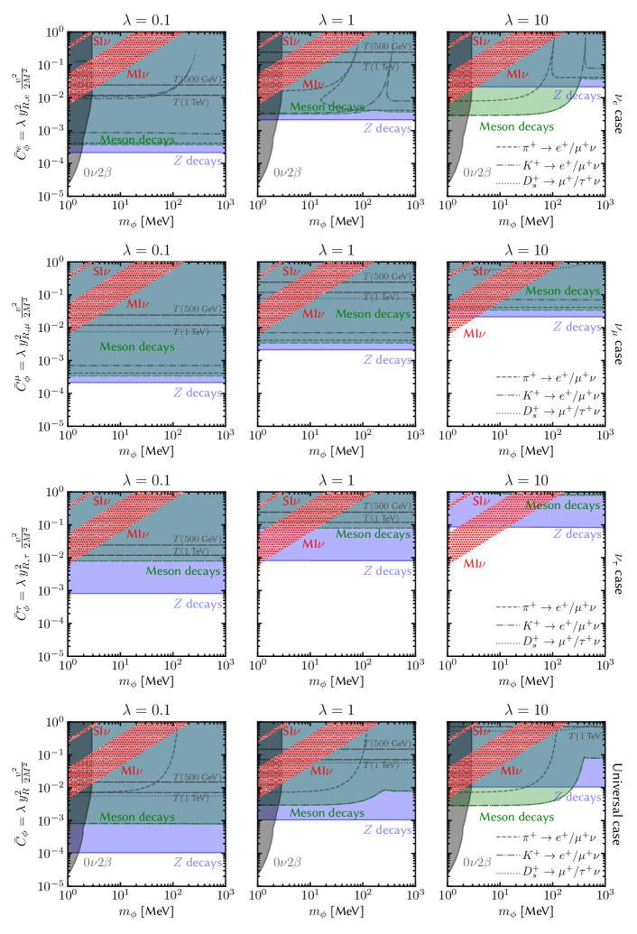
Figure 2: Exclusion regions for various cases of the inverse seesaw model in the $\bar{C}_{\phi}^{(f)}-m_{\phi}$ plane. First-, second-, and third-row plots correspond to the flavor-specific $e$-, $\mu$-, and $\tau$-case, respectively. Fourth-row plots correspond to the “universal” case. Each column shows the case of different values of $\lambda=0.1,1,10$. The colored regions are excluded at $90\%$ CL: in purple the combined constraints from $Z$ decays, in green the combined constraints from meson decays, and in grey the constraints from neutrinoless double-$\beta$ decay Blum et al. (2018). Dashed lines indicated in the legend show the constraints from each meson sector separately. The red-dotted regions are the preferred $1\sigma$ regions of the CMB fit. The horizontal, dashed lines show the constraint from the $T$-parameter when the heavy-neutrino scale is $M=500$ GeV and $M=1$ TeV.

In the previous section we considered the particle-physics constraints in conjunction with the preferred region from the CMB fit within the mostly model-independent framework of SMEFT. In concrete models, the SMEFT Wilson coefficients can be correlated, reducing the number of free parameters and leading to correlated signals. To illustrate this, we now study the phenomenology of the inverse-seesaw model from section II.2.2. Similarly to before we consider separately the three “flavor-specific” cases and the “universal” one. In each case, we vary the $\phi$ mass and the effective Majoron coupling to neutrinos, $\bar{C}_{\phi}^{(f)}$, while keeping the UV coupling $\lambda$ fixed. As representative values for $\lambda$ we take $\lambda=0.1,\,1,\,10$. We consider the case $m_{\phi}>1$ MeV. Smaller values of $m_{\phi}$ are constrained by BBN Ng and Beacom (2014); Blinov et al. (2019).

In figure 2, we show the resulting constraints in the $\bar{C}_{\phi}^{(f)}-m_{\phi}$ plane. First-, second-, and third-row plots correspond to the flavor-specific $e$-, $\mu$-, and $\tau$-case, respectively. Plots of the fourth row correspond to the “universal” case. Plots of each column present the case of different values of $\lambda$. The colored regions are excluded at $90\%$ CL: in purple the combined constraints from $Z$ decays, in green the combined constraints from meson decays, and in grey the constraints from neutrinoless double-$\beta$ decay Blum et al. (2018). Dashed lines indicated in the legend show the constraints from each meson sector separately, i.e., from $\pi^{+}$, $K^{+}$, and $D_{s}^{+}$ decays. The red-dotted regions are the preferred $1\sigma$ regions of the CMB fit. The horizontal, dashed lines show the constraint from the $T$-parameter when the heavy-neutrino scale is $M=500$ GeV and $M=1$ TeV.

By inspecting figure 2 we recover some of the conclusions from the SMEFT analysis of the previous section.

• The best-fit regions of the CMB fit cannot be accommodated in the “flavor-specific” $\nu_{e}$ and “universal” cases.

• While the SI$\nu$ scenario is strongly disfavoured, the particle-physics constraints are compatible with the MI$\nu$ scenario in the “flavor-specific” $\nu_{\mu}$ and $\nu_{\tau}$ cases, but only for masses $m_{\phi}\lesssim 10$ MeV and large values of $\lambda$, i.e., $\lambda\gtrsim 1$, close to its perturbativity limit. This in turn implies that this scenario must have a cut-off close to the mass scale of exotic fermions.

• The non-trivial structure of the $\pi^{+}$ (dashed-dotted lines) and $K^{+}$ (dashed lines) constraints in the $\nu_{e}$ and “universal” case is due to the interplay between the two-body decays, which suppresses the branching ratio BR$(M\to\ell\nu(\phi))$, and the three-body decay, which enhances it.

• The scenario is being further tested at colliders by searches for the heavy neutrinos. The analyses, for example Refs. Aad et al. (2015); Sirunyan et al. (2018), typically search for the heavy-neutrino decays to $W$s and either electrons or muons, thus placing limits on the mass of the heavy neutrino for the flavor specific $e$ and $\mu$ cases, and not the $\tau$ case. In both $e$ and $\mu$ case, the present limits are rather weak, i.e., $M\gtrsim 100$ GeV Aad et al. (2015); Sirunyan et al. (2018) for a mixing of the order $10^{-2}-10^{-3}$ between light and heavy neutrinos.

Qualitatively the results of this section are similar to Ng and Beacom (2014); Blinov et al. (2019), but there are important differences. In particular, the constraints from $Z$ decays, which are dictated by gauge invariance, provide powerful constraints. They restrict the allowed parameter-space of the $\nu_{\tau}$ “flavor-specific” case more than meson decays. The allowed region corresponds to large couplings, close to their perturbativity bound.

V Conclusions

Motivated by the approach of using neutrino self-interactions to address the tension in the $H_{0}$ measurement, we investigated the experimental constraints on this scenario. In contrast to previous studies on this setup, we began with an effective-field-theory framework that respects the full Standard Model gauge symmetry. This is important as many of the constraints are from experiments performed around the electroweak scale, where the effect of electroweak symmetry is essential. In addition to the SMEFT framework, we have also considered a UV completion within an inverse-seesaw type model. We performed an careful derivation of the constraints from $Z$ decay, $T$-parameter, and meson decays. We also took into account the limits from the search of neutrinoless double-$\beta$ decay and BBN. The constraints depends on the flavor structure of the couplings. To illustrate this, we considered two scenarios. In one of them, the self-interaction act in a “flavor universal” way to all flavors of neutrinos. In the other one, there is only interaction between one specific flavor species.

We showed that, in the “flavor universal” case, the neutrino self-interaction as a solution to the $H_{0}$ problem is strongly disfavored. Only the “flavor-specific” $\nu_{\mu}$ and $\nu_{\tau}$ cases in the MI$\nu$ scenario may be provide a solution. However, the scalar mass must be low and the scalar–neutrino couplings large, close to their perturbativity limits. The SI$\nu$ scenario is strongly disfavoured.

Future experimental searches are promising in further testing these scenarios. The experimental measurements considered in this paper will be improved significantly at on-going and future facilities. The scenarios under consideration also point to new particles, for example the new heavy neutrinos, not far away from the weak scale. They can be searched for directly in the upcoming LHC runs and at potential higher-energy colliders.

VI Acknowledgements

We would like to thank Sam McDermott and Massimiliano Lattanzi for useful discussions. LTW is supported by the DOE grant DE-SC0013642. KFL is supported in part by the Heising-Simons Foundation, the Simons Foundation, and National Science Foundation Grant No. NSF PHY-1748958 and acknowledges the hospitality of the Enrico Fermi Institute, where this work was initiated. ES is supported by the Fermi Fellowship at the Enrico Fermi Institute and by the U.S. Department of Energy, Office of Science, Office of Theoretical Research in High Energy Physics under Award No. DE-SC0009924 and by the Swiss National Science Foundation under contract 200021–178999.

References

- Aghanim et al. (2018) N. Aghanim et al. (Planck) (2018), eprint 1807.06209.
- Riess et al. (2018) A. G. Riess, S. Casertano, D. Kenworthy, D. Scolnic, and L. Macri (2018), eprint 1810.03526.
- Shanks et al. (2018) T. Shanks, L. Hogarth, and N. Metcalfe (2018), eprint 1810.07628.
- Riess et al. (2019) A. G. Riess, S. Casertano, W. Yuan, L. M. Macri, and D. Scolnic, Astrophys. J. 876, 85 (2019), eprint 1903.07603.
- Wong et al. (2019) K. C. Wong et al. (2019), eprint 1907.04869.
- Kreisch et al. (2019) C. D. Kreisch, F.-Y. Cyr-Racine, and O. Doré (2019), eprint 1902.00534.
- Blinov et al. (2019) N. Blinov, K. J. Kelly, G. Z. Krnjaic, and S. D. McDermott (2019), eprint 1905.02727.
- Gelmini and Roncadelli (1981) G. Gelmini and M. Roncadelli, Phys. Lett. B 99, 411 (1981).
- Oldengott et al. (2017) I. M. Oldengott, T. Tram, C. Rampf, and Y. Y. Y. Wong, JCAP 1711, 027 (2017), eprint 1706.02123.
- Lancaster et al. (2017) L. Lancaster, F.-Y. Cyr-Racine, L. Knox, and Z. Pan, JCAP 07, 033 (2017), eprint 1704.06657.
- Archidiacono and Hannestad (2014) M. Archidiacono and S. Hannestad, JCAP 07, 046 (2014), eprint 1311.3873.
- Cyr-Racine and Sigurdson (2014) F.-Y. Cyr-Racine and K. Sigurdson, Phys. Rev. D 90, 123533 (2014), eprint 1306.1536.
- Huang et al. (2018) G.-y. Huang, T. Ohlsson, and S. Zhou, Phys. Rev. D 97, 075009 (2018), eprint 1712.04792.
- Farzan (2003) Y. Farzan, Phys. Rev. D67, 073015 (2003), eprint hep-ph/0211375.
- Kachelriess et al. (2000) M. Kachelriess, R. Tomas, and J. W. F. Valle, Phys. Rev. D62, 023004 (2000), eprint hep-ph/0001039.
- Gando et al. (2012) A. Gando et al. (KamLAND-Zen), Phys. Rev. C86, 021601 (2012), eprint 1205.6372.
- Arnold et al. (2018) R. Arnold et al., Eur. Phys. J. C78, 821 (2018), eprint 1806.05553.
- Britton et al. (1994) D. I. Britton et al., Phys. Rev. D49, 28 (1994).
- Lazzeroni et al. (2013) C. Lazzeroni et al. (NA62), Phys. Lett. B719, 326 (2013), eprint 1212.4012.
- Lazzeroni et al. (2011) C. Lazzeroni et al. (NA62), Phys. Lett. B698, 105 (2011), eprint 1101.4805.
- Lessa and Peres (2007) A. Lessa and O. Peres, Phys. Rev. D 75, 094001 (2007), eprint hep-ph/0701068.
- Bakhti and Farzan (2017) P. Bakhti and Y. Farzan, Phys. Rev. D 95, 095008 (2017), eprint 1702.04187.
- Brdar et al. (2020) V. Brdar, M. Lindner, S. Vogl, and X.-J. Xu (2020), eprint 2003.05339.
- Abbiendi et al. (2004) G. Abbiendi et al. (OPAL), Eur. Phys. J. C33, 173 (2004), eprint hep-ex/0309053.
- Fileviez Perez et al. (2008) P. Fileviez Perez, T. Han, G.-y. Huang, T. Li, and K. Wang, Phys. Rev. D 78, 015018 (2008), eprint 0805.3536.
- Cai et al. (2018) Y. Cai, T. Han, T. Li, and R. Ruiz, Front. in Phys. 6, 40 (2018), eprint 1711.02180.
- Grzadkowski et al. (2010) B. Grzadkowski, M. Iskrzynski, M. Misiak, and J. Rosiek, JHEP 10, 085 (2010), eprint 1008.4884.
- Dias et al. (2012) A. Dias, C. de S.Pires, P. Rodrigues da Silva, and A. Sampieri, Phys. Rev. D 86, 035007 (2012), eprint 1206.2590.
- Law and McDonald (2013) S. S. Law and K. L. McDonald, Phys. Rev. D 87, 113003 (2013), eprint 1303.4887.
- Mohapatra and Valle (1986) R. Mohapatra and J. Valle, Phys. Rev. D 34, 1642 (1986).
- Ma (1987) E. Ma, Phys. Lett. B 191, 287 (1987).
- Ma (2009) E. Ma, Phys. Rev. D 80, 013013 (2009), eprint 0904.4450.
- Bazzocchi (2011) F. Bazzocchi, Phys. Rev. D 83, 093009 (2011), eprint 1011.6299.
- Brivio et al. (2017) I. Brivio, Y. Jiang, and M. Trott, JHEP 12, 070 (2017), eprint 1709.06492.
- Barbieri et al. (2004) R. Barbieri, A. Pomarol, R. Rattazzi, and A. Strumia, Nucl. Phys. B703, 127 (2004), eprint hep-ph/0405040.
- Alonso et al. (2014) R. Alonso, E. E. Jenkins, A. V. Manohar, and M. Trott, JHEP 04, 159 (2014), eprint 1312.2014.
- Jenkins et al. (2014) E. E. Jenkins, A. V. Manohar, and M. Trott, JHEP 01, 035 (2014), eprint 1310.4838.
- Kolb and Turner (1990) E. W. Kolb and M. S. Turner, Front. Phys. 69, 1 (1990).
- Gondolo and Gelmini (1991) P. Gondolo and G. Gelmini, Nucl. Phys. B360, 145 (1991).
- Tanabashi et al. (2018) M. Tanabashi et al. (Particle Data Group), Phys. Rev. D98, 030001 (2018).
- Blum et al. (2018) K. Blum, Y. Nir, and M. Shavit, Phys. Lett. B785, 354 (2018), eprint 1802.08019.
- Arnold et al. (2014) R. Arnold et al. (NEMO-3), Phys. Rev. D89, 111101 (2014), eprint 1311.5695.
- Ng and Beacom (2014) K. C. Y. Ng and J. F. Beacom, Phys. Rev. D90, 065035 (2014), [Erratum: Phys. Rev.D90,no.8,089904(2014)], eprint 1404.2288.
- Aad et al. (2015) G. Aad et al. (ATLAS), JHEP 07, 162 (2015), eprint 1506.06020.
- Sirunyan et al. (2018) A. M. Sirunyan et al. (CMS), Phys. Rev. Lett. 120, 221801 (2018), eprint 1802.02965.