Y. Faenza, S. Gupta, X. Zhang

Filtering the Feeder Effect in Public School Admissions Reducing the Feeder Effect in Public School Admissions:
A Bias-aware Analysis for Targeted Interventions

Yuri Faenza Columbia University, New York, NY
yf2414@columbia.edu Swati Gupta Georgia Institute of Technology, Atlanta, GA
swatig@gatech.edu Xuan Zhang Columbia University, New York, NY
xz2569@columbia.edu

Traditionally, New York City’s top 8 public schools select candidates solely based on their scores in the Specialized High School Admissions Test (SHSAT). These scores are known to be impacted by socioeconomic status of students and test preparation received in “feeder” middle schools, leading to a massive filtering effect in the education pipeline. For instance, around 50% (resp. 80%) of the students admitted to the top public high schools in New York City come from only 5% (resp. 15%) of the middle schools. The classical mechanisms for assigning students to schools do not naturally address problems like school segregation and class diversity, which have worsened over the years. The scientific community, including policy makers, have reacted by incorporating group-specific quotas, proportionality constraints, or summer school opportunities, but there is evidence that these can end up hurting minorities or even create legal challenges. We take a completely different approach to reduce this filtering effect of feeder middle schools, with the goal of increasing the opportunity of students with high economic needs. We model a two-sided market where a candidate may not be perceived at their true potential, and is therefore assigned to a lower level than the one (s)he deserves. We propose and study the effect of interventions such as additional training and scholarships towards disadvantaged students, and challenge existing mechanisms for scholarships. We validate these findings using SAT scores data from New York City high schools. We further show that our qualitative takeaways remain the same even when some of the modeling assumptions are relaxed.

bias, admissions, interventions, matchings, two-sided market

1 Introduction

Bias and the disparity in opportunities are believed to play a major role in the access to education at different levels (Quinn Capers et al. 2017). It is known that opportunities at middle school admissions dictate high school admissions, which in turn impact pathways to higher studies (Corcoran and Baker-Smith 2018). Selection however starts much earlier, with gifted and talented programs screening students as young as 4 years old; these tests often see a small number of minorities succeeding Shapiro (2019a). In this work, we are motivated by high-school admissions in large cities such as New York City, which has a very extensive public school system with over a million students currently enrolled. In particular, every year roughly 80,000 students wish to join one of the 700 high school programs. The most sought after top public schools select candidates solely based on their scores in the Specialized High School Admissions Test (SHSAT) (New York City Department of Education NYC DOE). However, such scores are known to be impacted by socioeconomic status of students  (Lovaglia et al. 1998) and test preparation received in middle school (Corcoran and Baker-Smith 2018, Shapiro February 06, 2019). Since minorities tend to cluster in middle and high schools of lower quality (Boschma and Brownstein 2016), they are already at a disadvantage in high school admissions, which then reflects in under-representation in higher education programs (Ashkenas et al. 2017). This results in a massive filtering effect in high school admissions: 50% (resp. 80%) of the students admitted to the top public high schools in New York City come from only top 5% (resp. 15%) of the middle schools (Corcoran and Baker-Smith 2018). Our goal in this work is to consider high school admissions stage of the education pipeline, and investigate data-driven interventions (like summer schools or preparatory courses) which can reduce the extent of the minority filtering effect.

The most common way to model admission to schools is through a two-sided market, with the two sides being schools and students, respectively, and each agent having an ordered preference on the agents from the other side of the market that are considered acceptable. This model has been used to match doctors to hospitals by the National Residency Matching Program since 1960s, and it has gained widespread notoriety when Abdulkadiroğlu et al. (2005) reformed the admission process for New York City public high schools in 2003. Since 2003, admission is centralized and has been (essentially) governed by the classical Gale-Shapley / Deferred Acceptance algorithm (Gale and Shapley 1962). The simplicity of the algorithm, as well as the drastic improvement over the quality of the matches it provides when compared to the pre-2003 method, led to academic and public acclaim, and spurred applications in many other systems (see, e.g., Biró (2008)). However, this mechanism does not naturally address problems like school segregation and class diversity, which have worsened and become more and more of a concern in recent years (Kucsera and Orfield 2014, Shapiro March 26, 2019, Shapiro and Lai June 03, 2019). The scientific community, including policy makers, has reacted by incorporating in the mathematical model group-specific quotas, proportionality constraints (Biró et al. 2010, Nguyen and Vohra 2019, Tomoeda 2018), and starting summer school pre-training programs, but there is evidence that adding such constraints may even hurt minorities they were meant to help (Hafalir et al. 2013) or create legal challenges. For example, in 2003, University of Michigan’s attempt to add 12 points of “diversity” on a 150 point scale to promote admissions of underrepresented minorities was met with a lawsuit, which was ultimately decided not in favor of race-based modifications of ranking of students Gratz v. Bollinger (2003).

We take a completely different approach to reduce the filtering effect of feeder middle schools, with the goal of increasing the opportunity of students with high economic needs rather than changing admission policies of educational institutions. We model a two-sided market where a candidate may not be perceived at their true potential, and is therefore assigned to a lower level than the one (s)he deserves. We propose and study the effect of interventions such as additional training and scholarships towards disadvantaged students, quantifying the effect of those mechanisms and identifying the population they should be targeted to. One of our key findings is that when scholarships are provided to students, one needs to take into account the distribution of grades or abilities observed amongst the applicants. The students who would likely benefit the most from additional training resources, for instance, are the average performing (rather than top) disadvantaged students when their abilities is close to Pareto-distributed Clauset et al. (2009), Kleinberg and Raghavan (2018), thus challenging currently existing mechanisms. When the abilities are Gaussian-distributed, most of our qualitative takeaways stay the same, with the difference that scholarships should target minority students closer to the top.

We validate these findings using SAT scores data from New York City high schools and data on the economic need indices of middle schools. We further show that our qualitative takeaways remain the same even when some of the modeling assumptions are relaxed. We summarize our model and contributions next.

1.1 The model

We give here a high-level view of our model, and defer the details and a comparison with models from the literature to Section 2. We assume that both sides of the market (to which we refer as schools and students henceforth) form continuous sets. Every student is assigned a real number, to which we refer as the (true) potential of the student. The schools are however only aware of a different number, to which we refer as the perceived potential. We assume the population of students is divided into two sets, $G_{1}$ and $G_{2}$. For a student from $G_{1}$, his/her potential and perceived potential coincide, while for a student from $G_{2}$, his/her perceived potential equals to the potential multiplied by a constant $\beta\in(0,1]$. Students from $G_{2}$ form a $p$ fraction of the total population, with $p\in[0,1]$. As we alluded to in the introduction, there could be multiple causes why this bias is perceived: the scholastic career of the student, their attitude, their prior access to high-quality education, the tools schools use to evaluate them, etc.

Models with a multiplicative bias have received recent attention in the literature Kleinberg and Raghavan (2018). Moreover, as we discuss next, their application in the school choice market is supported by data. Consider for instance the SAT scores across New York City middle schools. Using data on middle schools’ economic need index as a proxy for students’ economic need index, we divide students into two groups, with $50\%$ of the students in the $G_{1}$ group and $50\%$ in the $G_{2}$ group (i.e., $p=0.5$). By estimating the “bias” factor across the two groups of students as $\beta=\frac{1}{1.25}=0.8$, then the distribution of real potential between $G_{1}$ and $G_{2}$ have a large overlap, see Figures 1(a), 1(b).

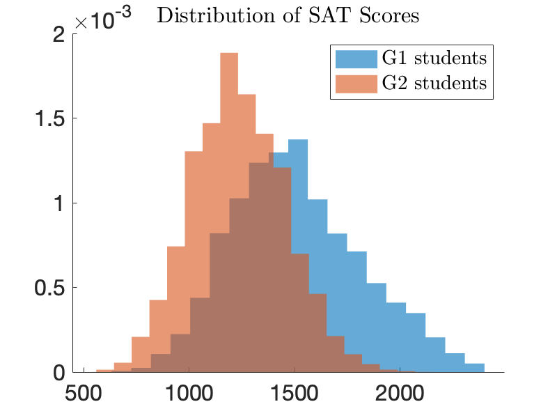
(a) Original SAT Scores

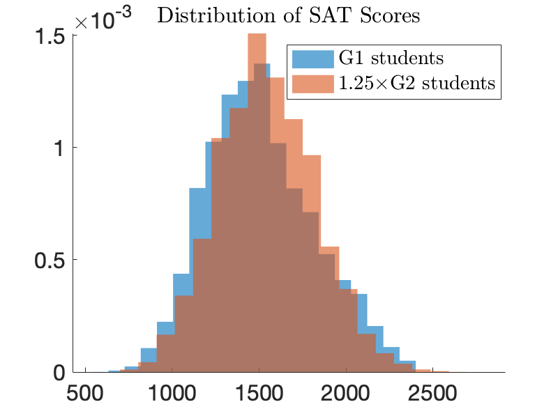
(b) Debaised SAT Scores

Figure 1: Distribution of SAT scores across students in schools with “low economic need index” (group $G_{1}$) versus the distribution of SAT scores across students in schools with “high economic need index” (group $G_{2}$). We estimate the bias factor $\beta=\frac{1}{1.25}=0.8$.

In our model, we next consider the schools’ ranking of students based on their perceived potentials. Hence, all schools share the same ranking of students. One possible interpretation for the perceived potentials is students’ standardized test score, as is the case of top high schools in New York City. Similarly, universities in China and India rank students in an unanimous order according to their test scores in the college-entrance exam (Wikipedia contributors 2019). We further assume that there is a unique, strict ranking of schools, that every student agrees on. This could be interpreted as one of the many available rankings of schools (such as US News Rankings), or as a shared perception of which schools are the best. Although this assumption abstracts out many considerations that may be important for students (e.g. proximity of a school (Burgess et al. 2015) or constraints on the size of preference lists (Calsamiglia et al. 2010)), it is known that rankings have a huge impact on the colleges that students select Luca and Smith (2013). As an example, it is currently largely acknowledged that, among top public scientific high schools in New York City, Stuyvesant is the most selective and demanded, followed by Bronx Science and Brooklyn Tech (Corcoran and Baker-Smith 2018).

We consider two different choices on the distribution of students’ potentials. First, following the recent work on multiplicative bias by Kleinberg and Raghavan (2018), Celis et al. (2021, 2020), Salem and Gupta (2020) we assume that the potentials of students can be distributed following a Pareto (power law) distribution with support $[1,\infty)$. There has been much empirical work (see, e.g., Clauset et al. (2009)) supporting the statement that the achievement of individuals in many professions can be well approximated using such distributions with a small, positive power-law exponent, denoted in the following by $\alpha$. Second, we also allow the potentials of students to be Gaussian-distributed. This motivated by the fact that the scores of many tests, for instance SAT, follow the Gaussian distribution Taube and Linden (1989). As already discussed, standardized tests play a major role in school admission. Our analysis of the Gaussian distribution is canonical, in the sense that, in case the student performance is observed to be distributed as any other distribution, the same framework can be used to find the most impactful segment of disadvantaged students for targeting interventions.

Because of the structure of our model, most classical concepts of efficiency and fairness are satisfied by the matching where students are admitted to schools in order of their potentials, while we assume that in the biased setting, students are matched according to their perceived potentials (see Section 2 for formal definitions). This paper is devoted to understand how different those two matchings are (in terms of a variety of measures) and what interventions can be put in place to reduce this difference through the reduction of bias. We interpret such interventions, e.g., conducting student interviews, providing additional training, building communities for students, as limited-resource activities that can reveal the true potential for certain students.

1.2 Summary of Contributions

We next present the key questions we explore in this work, and concurrently discuss the analytic answer we show when the potentials of students follow the Pareto distribution. We later discuss how the answers change when the potential of students follow the Gaussian distribution instead.

1.2.1 Pareto-Distributed Student Performance.

Q1. Impact on Students in terms of School Rank:

How costly is bias for students amongst the advantaged group $G_{1}$ and the disadvantaged group $G_{2}$? Can a student be placed in a school much worse than the one (s)he deserves, because of bias?

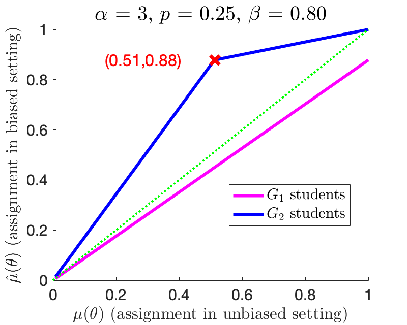
Figure 2: Schools students “should” versus “actually” attend. The green dotted line is a line of slope one, representing the place a student should be placed on the figure if there are no bias in the system.

We formally investigate this question in Section 3.1. We observe that all $G_{2}$ students are assigned to schools that are worse than what they actually deserve, with some $G_{2}$ students being assigned to significantly lower ranked schools (e.g., see Figure 2, where for Pareto-distributed potentials, a student who should have been matched to a normalized school rank of 0.51, actually ends up getting matched to a normalized school rank of 0.88 under $\beta=0.8$). Quantitatively, the presence of bias impacts the average students the most – where they are pushed to significantly lower ranked schools.

Let us call, for any student, the difference between the rank of the matched school in the biased setting and the rank of the matched school in the unbiased setting (when schools observe the true potentials) with the term displacement. We show that the maximum displacement is impacted by the fraction of disadvantaged students in the total population. If the fraction of disadvantaged students $p$ decreases, then the maximum displacement they experience increases significantly. Moreover, the impact is not linear or symmetric across the two groups of advantaged and disadvantaged students.

Q2. Impact on Schools in Diversity and Quality of Admitted Students:

How costly is bias for schools? Would the utility of schools – that we define to be the average potential of assigned students – be much lower when $G_{2}$ students are perceived with lower potentials? In addition, how does the presence of bias affect diversity at schools?

We give a formal answer to these questions in Section 3.2. Qualitatively, we show that, in contrast to the negative impact of bias on the school matches of $G_{2}$ students, the impact on the utilities of schools is negligible for all schools other than the lowest ranked schools. Here the utility of a school is defined to be the average potential of the students that are enrolled in it. If this what schools wish to maximize, they therefore seem to have little incentive to change the way admissions are performed. This phenomenon happens because for each school, although the average potential of assigned $G_{1}$ students is lower than it should be, its assigned $G_{2}$ students have much higher true potentials. And thus, the toll on the utility due to unqualified $G_{1}$ students is partially canceled out by the overqualified $G_{2}$ students and the net effect is minimal. On the other hand, some lower ranked schools that only admit $G_{2}$ students fare better in the biased setting (since they admit over-qualified $G_{2}$ candidates). We also discuss the effect of bias on the diversity of school cohorts.

Q3. School-specific Interventions:

What can schools do to remove bias (i.e., help $G_{2}$ students reveal their true potentials)? How much can a school’s utility change from interventions such as additional interviews of disadvantaged students?

This question is investigated in Section 4.1. We consider the intervention where schools conduct extensive analysis of students who are slightly below their admission criteria (i.e., students who are originally assigned to slightly lower ranked schools), with the goal of reviewing their true potentials. We call this process interviewing, although such interventions can include several alternative measure of the students’ abilities. Given that conducting interviews takes resources, we assume that every school has certain interview capacities. We analyze the change in schools’ utility under such interviewing scheme, and show that the only scenario when a school has a significant interest to interview is when it is the only one that does so, and moreover it does not belong to either the best, nor the worst schools.

Hence, a decentralized process that leaves to schools the choice of interviewing does not look very promising since the gain in utility for each individual school is minimal. Given that there is an overlap in the students that similarly ranked schools interview, students have to go through many interviews and reveal their true potentials to the schools separately. Moreover, being aware of interview dates and able to attend them has traditionally been another source of discrimination, for instance, in New York City high schools (Shapiro 2019b).

We next explore a more societal level, centralized form of intervention, which can be thought of, for instance, as providing extra training/resources, developing problem solving groups, or team building exercises. The idea that disparity in opportunities should be fought by expanding the access to test preparation has been gaining traction in the past years. For instance, in New York City, there has been growing support for free SHSAT preparation for middle-school students (Education Equity 2020).

Q4. Central Interventions such as Trainings:

What can the government or other public agencies do to remove bias, i.e., what are some school-independent interventions? How much can students benefit from such interventions? Who should such interventions target given limited resources?

We generically call this societal interventions vouchers, and investigate their effect in Section 4.2. We assume that only $G_{2}$ students will use vouchers, and this will have the effect of removing their bias. This is justified by the fact that $G_{1}$ students should already have had access to, say, extra training (this is why they were $G_{1}$ students to begin with). We investigate two measures of unfairness or mistreatment (i.e., positive displacement) of $G_{2}$ students motivated by axiomatically justified notions of (in)equality (Kumar and Kleinberg 2000, Bertsimas et al. 2011), and for each one, we give explicit formula on who are the $G_{2}$ students that should be debiased in order to minimize this measure of mistreatment. The two measures we consider are 1) the maximum mistreatment (in absolute value or in lexicographical order) and 2) the average mistreatment of all mistreated $G_{2}$ students. In both cases, informally speaking, the students we should target are those whose potential is close to that of the most misplaced student, hence students with average potential. We find that, in contrast to targeted interviews by schools, distributing vouchers or training resources based on observed potentials of students are more effective.

These results complement the growing stream of papers that characterize trade-offs between multiple metrics of fairness, specifically for statistical measures of fairness such as calibration across groups, balance for positive class, and balance for negative class (Kleinberg et al. 2017). In contrast to statistical measures, where there exist impossibility results of satisfying multiple fairness metrics simultaneously (even approximately), we show that the average as well as maximum mistreatment is minimized in our problem by targeting a similar set of students.

1.2.2 Gaussian-Distributed Student Performance and Extensions.

We next discuss if our qualitative takeaways still hold if the assumptions of Pareto-distributed performance are changed to other distributions such as Gaussian, and if some of the modeling assumptions are relaxed.

Q5. Impact on Students and Schools, and Interventions:

Do the takeaways from answers to questions Q1-Q4 still hold if the potentials of students follow a Gaussian distribution or some other distribution observed in data?

Quantitatively, we extend our analysis to general distributions in Section 5. Qualitatively, most takeaways remain, but there are some differences. From schools’ perspective, we find that the top schools are distinctly affected by bias in the system, and therefore, individually each school has an incentive to conduct interview. However, when all the schools interview, then the change in utility is negligible compared to the status-quo. Hence, one should again rely on a central authority for debiasing the students. Under both measures discussed in Q4, vouchers should be provided to middle-top students – i.e., students above average but not top students. This is different from the case of the Pareto distribution, where we target students with median performance.

Q6. Extensions with Relaxed Assumptions:

Can the assumptions made in our model for mathematical tractability can be relaxed, while keeping the results qualitatively similar? In particular, what if we move from a continuous to a discrete model, assume $\beta$ non-constant, or assume that not all students that are offered a voucher will use it? What if the majority students face bias, instead of minority, i.e., $p>0.5$?

We investigate these questions empirically in Section 6, and show that most qualitative takeaways remain the same even under those perturbed assumption. Our experiments provide evidence that our results extend well beyond the model studied in this paper, and can be impactful in more realistic settings, where our assumptions hold approximately.

We believe our work asks interesting questions that can help understand the impact of inconsistency in evaluation mechanisms across demographic groups.

1.3 Discussion

Our key qualitative takeaways are important and speak to a much ingrained systemic problem that limits access to opportunities – how can one understand the impact of bias on societal practices and systematically account for biases in the real world. Indeed, resources available for meaningful interventions in an existing system are limited, and there is resistance to change: for instance, a 2019 plan supported by New York City’s mayor to eliminate the entrance exam to top public high schools has failed to gain enough support, and was not approved by the New York State government (Shapiro and Wang 2019). Thus, our focus is on understanding the impact of minimally invasive use of targeted resources, as opposed to changing the matching mechanism itself. From our analysis, we are able to highlight the following qualitative properties using simple models of bias and matching mechanism:

1. Disparate Impact: The disparity in admissions is experienced much more by the group of students who face biases and stereotypes, compared to the marginal advantage of students from the non-stereotyped group.

2. Interventions: Decentralized interventions at the individual-school level are not as impactful from schools’ perspective and thus schools have little incentive for change.

3. Resources: Centralized debiasing interventions are meaningful tools to address the disparity. Which students should be the target of those interventions depend on the assumption on the distribution of student potentials and not the measure of fairness under consideration. The optimal set of students to target oscillates between the average students (in the case of Pareto distribution) and average-top students (in the case of Gaussian distribution). Hence, in settings where we can assume that the student potential is indeed Pareto distributed (e.g., applicants to schools with a focus on a specific curriculum), our findings support the idea of including average students in the allocation of vouchers.

These takeaways are a first step, and in no way address all the systemic problems in school admission process – such as access to counselors, transport to schools or familial support towards education. But they do help us understand the most impacted student groups, and provide a mathematical basis to the public policy communities to debate existing scholarship mechanisms. Future work include further relaxations of the assumptions, such assuming that students have slightly different rankings of schools, investigation on different distributions of students’ potentials, as well as debiasing mechanisms that satisfy individual fairness (see the discussion at the end of Section 4.2).

2 A continuous matching market

We introduce a simple matching market, where students rank schools following a unique strict order, and schools rank students following a unique order. Both schools and students are continuous sets. We let the student population be a set $\Theta$, and we associate to $\Theta$ a probability distribution on the potentials of students. For each student $\theta\in\Theta$, we use $Z(\theta)$ to denote his/her true potential. Unless otherwise stated, we assume $Z(\Theta)\sim\text{Pareto}(1,\alpha)$, and thus, all students have potentials at least $1$. We let $\mu:\Theta\rightarrow[0,1]$ be the ranking function based on students’ true potentials, with rankings normalized to be between $0$ and $1$, and a student $\theta$ with a smaller value of $\mu(\theta)$ is a student who has higher potential. Hence for $\theta,\theta^{\prime}\in\Theta$, whenever $Z({\theta^{\prime}})>Z(\theta$), we have $\mu(\theta^{\prime})<\mu(\theta)$. Students with the same potential are ranked at the same level.

We assume that $p$ fraction of the students belong to Group 2 ($G_{2}$). $G_{2}$ students are the ones whose perceived potentials are biased by a constant multiplicative factor $\beta\in(0,1]$. Students who are not in Group 2 are called Group 1 ($G_{1}$) students. Their perceived potentials are exactly their true potentials and they account for $1-p$ proportion of the population.

We let $\widehat{Z}(\theta)$ denote the perceived potential of a student $\theta\in\Theta$. That is, if $\theta\in G_{1}$, then $\widehat{Z}(\theta)=Z(\theta)$; otherwise, $\widehat{Z}(\theta)=\beta Z(\theta)$. For $G_{1}$ students, the cdf (cumulative distribution function) of their perceived (or equivalently true) potentials is denoted by $F_{1}$. Similarly, let $F_{2}$ denote the cdf of the perceived potentials of $G_{2}$ students. Since $Z(\Theta)\sim\text{Pareto}(1,\alpha)$, we have

$$F_{1}(t)=1-t^{-\alpha};\qquad F_{2}(t)=1-\beta^{\alpha}t^{-\alpha}.$$

Note that both function $F_{1}(\cdot)$ and $F_{2}(\cdot)$ take in the value of perceived potentials. Moreover, the domain of $F_{1}$ is $[1,\infty)$, whereas the domain of $F_{2}$ is $[\beta,\infty)$.

Let $\widehat{\mu}:\Theta\rightarrow[0,1]$ be the function that ranks students based on their perceived potentials, with again rankings normalized to be between $0$ and $1$. It is also convenient to define the ccdf (tail distribution) of students’ perceived potentials. That is, let $\bar{F}_{1}:=1-F_{1}$ and $\bar{F}_{2}:=1-F_{2}$ be the ccdf of their corresponding distributions. Then, for a student $\theta\in\Theta$, $\widehat{\mu}(\theta)$ counts the fraction of students whose perceived potential is higher than that of $\theta$. That is:

$$\widehat{\mu}(\theta)=\begin{cases}(1-p)\bar{F}_{1}(\widehat{Z}(\theta))+p\bar{F}_{2}(\widehat{Z}(\theta))&\text{ if }\theta\in G_{1},\\[2.84526pt] (1-p)\bar{F}_{1}(\widehat{Z}(\theta)\vee 1)+p\bar{F}_{2}(\widehat{Z}(\theta))&\text{ if }\theta\in{G_{2}},\end{cases}$$ (1)

where $\vee$ is the maximum operator. We say that student $\theta$ is assigned to school $\widehat{\mu}(\theta)$. Note that, when $\beta=1$ (i.e., no bias), formula (1) computes $\mu(\theta)$: $\mu(\theta)=\bar{F}_{1}(Z(\theta))$ for $\theta\in\Theta$.

Intuitively, $\mu(\theta)$ represents the school that student $\theta$ should be assigned to, whereas $\widehat{\mu}(\theta)$ is the school where student $\theta$ is actually assigned to due to bias. For $\gamma\in\{\mu,\widehat{\mu}\}$ and $s\in[0,1]$, we denote by $\gamma^{-1}(s)$ the set of students assigned to school $s$ under matching $\gamma$. In addition, we denote by $u_{\gamma}(s)$ the utility of school $s$ under matching $\gamma$, which is defined to be the average true potential of its assigned students. That is,

$$u_{\gamma}(s):=\int_{\theta\in\gamma^{-1}(s)\cap G_{1}}Z(\theta)dF_{1}(\widehat{Z}(\theta))+\int_{\theta\in\gamma^{-1}(s)\cap G_{2}}Z(\theta)dF_{2}(\widehat{Z}(\theta)).$$ (2)

Formally, we define a matching in this market to be a surjective measurable function $\gamma$ from $\Theta$ to $[0,1]$ (i.e., students to schools), such that the mass of students mapped to a set of school $S\subseteq[0,1]$ coincides with the standard Lebesgue measure of $S$. One can easily check that $\mu$ and $\widehat{\mu}$ defined above are matchings.

Discrete vs. continuous markets. Unlike traditional two-sided matching markets, where both sides are represented by discrete entities (Gale and Shapley 1962, Roth and Sotomayor 1992), we decided to define and study a continuous model. Our choice follows a recent trend in the literature (Arnosti 2019, Azevedo and Leshno 2016). We motivate and discuss it in detail in Appendix 7.

3 Analysis of the market

Our first goal is to understand how much bias affects agents in the market. In particular, we would like to answer the following question: what is the loss of efficiency for agents of the market when all students $\theta\in\Theta$ are assigned to school $\widehat{\mu}(\theta)$ instead of $\mu(\theta)$? We propose to measure this loss of efficiency in three ways: first, for students; second, for schools; and third, as a diversity measure.

3.1 Students’ perspective

Formally, we define $\widehat{\mu}(\theta)-\mu(\theta)$ to be the displacement of a student $\theta\in\Theta$. Note that if $\theta\in G_{1}$, the displacement is non-positive, and if $\theta\in G_{2}$, it is non-negative. The displacement can be easily calculated using the formulae for $\mu$ and $\widehat{\mu}$ given in (1).

Proposition 3.1

For any student $\theta\in G_{2}$, the displacement $\widehat{\mu}(\theta)-\mu(\theta)$ is given by:

$$\widehat{\mu}(\theta)-\mu(\theta)=\begin{cases}\displaystyle(1-p)\left({Z(\theta)}\right)^{-\alpha}\left(\beta^{-\alpha}-1\right)&\text{ if }Z(\theta)\geq\frac{1}{\beta},\\[2.84526pt] \displaystyle(1-p)\left(1-\left({Z(\theta)}\right)^{-\alpha}\right)&\text{ if }Z(\theta)\leq\frac{1}{\beta}.\end{cases}$$

And for any student $\theta\in G_{1}$, we have $\widehat{\mu}(\theta)-\mu(\theta)=\left(-p+p\beta^{\alpha}\right)\left({Z(\theta)}\right)^{-\alpha}.$ Thus, the maximum displacement of $(1-p)(1-\beta^{\alpha})$ is experienced by a $G_{2}$ student with potential $1/\beta$; and the most significant negative displacement of $-p(1-\beta^{\alpha})$ is experienced by a $G_{1}$ student with potential $1$.

One can think of this result intuitively in the following way. Starting from the top school, $G_{1}$ students gradually take more seats than they deserve, and thus gradually push $G_{2}$ students to worse schools than what they deserve. This process stops once all $G_{1}$ students are assigned to schools, and the only students that remain to be assigned are $G_{2}$ students. As a result, in lower ranked schools, all students are $G_{2}$ students. Hence, the difference in ranks of the schools $G_{2}$ students are matched to decreases towards the end. See Figure 2 for an example and Appendix 8.1 for additional figures.

3.2 Schools’ perspective

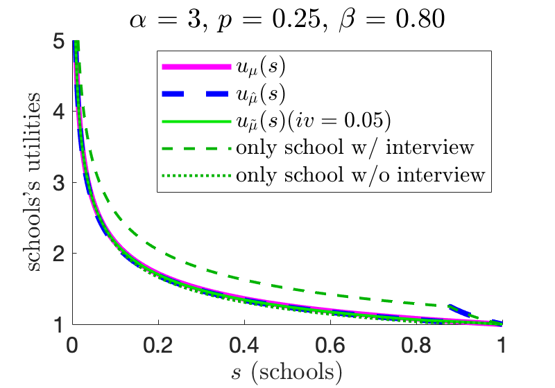
Figure 3: Comparing schools’ utilities in biased and unbiased setting; schools’ incentives of interviewing.

We discuss next the impact of bias on the average true potential of students accepted by a school. Let $s\in[0,1]$ denote the school that is ranked in the $s\times 100\%$ position among the continuous range of schools. As next proposition shows, the impact on the utilities of schools is negligible for all schools other than the lowest ranked schools. This is because for each school, although the average potential of assigned $G_{1}$ students is lower than it should be, its assigned $G_{2}$ students have much higher true potentials. And thus, the toll on the utility due to unqualified $G_{1}$ students is partially canceled out by the overqualified $G_{2}$ students and the net effect is minimal. On the other hand, some lower ranked schools that only admit $G_{2}$ students fare better in the biased setting (since they admit over-qualified $G_{2}$ candidates).

Proposition 3.2

For school $s$, its utility under the unbiased (resp. biased) models are respectively

$$u_{\mu}(s)=s^{-\frac{1}{\alpha}}\quad\hbox{ and }\quad u_{\widehat{\mu}}(s)=\begin{cases}\displaystyle\frac{1-p+p\beta^{\alpha}}{1-p+p\beta^{\alpha+1}}\left(\frac{s}{1-p+p\beta^{\alpha}}\right)^{-\frac{1}{\alpha}}&\text{ if }s\leq 1-p+p\beta^{\alpha},\\[2.84526pt] \displaystyle\left(\frac{s-(1-p)}{p}\right)^{-\frac{1}{\alpha}}&\text{ if }s>1-p+p\beta^{\alpha}.\end{cases}$$

We include a proof of Proposition 3.2 in Appendix 8.2. In Figure 3, we plot functions $u_{\mu}(s)$ and $u_{\widehat{\mu}}(s)$ (the two thick lines) as a visualization of the impact of bias on utilities of schools. Unlike the negative impact biases place on $G_{2}$ students, from schools’ perspective, the negative impact is negligible. Hence, from a operational perspective, it may be hard to convince schools to autonomously put in place mechanisms to alleviate the effect of bias. We analyze this more in detail in Section 4.1. In Appendix 8.3 we discuss how bias affects diversity in schools. In particular, we show that the proportion of $G_{2}$ students in higher ranked schools decreases significantly in the biased setting.

4 Mitigating the effect of bias

In this section, we discuss several alternatives for moderating the effect of bias. We call these actions bias mitigations, and investigate two of them. We remark that, in both interventions, no student $\theta\in G_{1}$ will be matched to a school worse than $\mu(\theta)$. This is because our interventions focus on helping (certain) $G_{2}$ students reveal their true potentials, hence for any $G_{1}$ student $\theta$, no student with potential lower than $Z(\theta)$ can have a perceived potential higher than $\widehat{Z}(\theta)=Z(\theta)$.

4.1 Interviewing

One way schools can act to mitigate the negative effects of bias is to spend resources that could reveal the true potentials of students. This could include, for instance, conducting extensive, holistic evaluations of the candidates and of their potential (rather than relying on the score on one test). For brevity, we call such a process interviewing. We assume that, when a school $s$ decides to conduct interviews, it is able to observe the true potentials of all $G_{2}$ students that were original matched to schools from $s$ to $s+iv_{s}$ for some constant $iv_{s}$ that represents the amount of students a school is able to interview. In this section, we investigate the incentives of conducting interviews from schools’ perspective: does interviewing allow a school to drastically improve the quality of the students it is matched to?

The first situation we consider is the simple case where all schools conduct interviews and all schools have the same interview capacity (i.e., $iv_{s}=iv$ for all schools $s$). Let $d^{i}_{1}(s)$ and $d^{i}_{2}(s)$ be the cutoffs in terms of true potentials each school $s$ has for $G_{1}$ and $G_{2}$ students respectively, and let $\widetilde{\mu}$ denote the resulting matching.

Proposition 4.1

The utilities of schools when all schools have interview capacity $iv$ is:

$$u_{\widetilde{\mu}}(s)=\begin{cases}\displaystyle\frac{(1-p)[d_{1}^{i}(s)]^{-(\alpha+1)}\cdot d_{1}^{i}(s)+p[d_{2}^{i}(s)]^{-(\alpha+1)}\cdot d_{2}^{i}(s)}{(1-p)[d_{1}^{i}(s)]^{-(\alpha+1)}+p[d_{2}^{i}(s)]^{-(\alpha+1)}}&\text{ if }d_{1}^{i}(s)>1\\[5.69054pt] \displaystyle d_{2}^{i}(s)&\text{ otherwise },\end{cases}$$

where

$$\begin{cases}d_{1}^{i}(s)=d_{2}^{i}(s)=\bar{F}_{1}^{-1}(s)&\text{if }\bar{F}_{1}\big{(}d(\min(1,s+iv))/\beta\big{)}\geq s\\[5.69054pt] \begin{cases}\displaystyle d_{2}^{i}(s)=d(\min(1,s+iv))/\beta\\[2.84526pt] \displaystyle d_{1}^{i}(s)=\bar{F}_{1}^{-1}\left(\frac{s-p\bar{F}_{1}(d_{2}^{i}(s))}{1-p}\right)\end{cases}&\text{if }\bar{F}_{1}\big{(}d(\min(1,s+iv))/\beta\big{)}<s\end{cases}$$

A proof of Proposition 4.1 is given in Appendix 9.1. The utilities of schools under this first situation, i.e., $u_{\widetilde{\mu}}(s)$, with $iv=0.05$ are plotted in Figure 3. We consider two additional situations, corresponding to the two additional lines in the figure. The dashed line represents the utility of each school $s$ if $s$ is the only school that interviews students. In this case, school $s$’s utility is $d(s)/\beta$. On the contrary, the dotted captures the utility of school $s$ when $s$ is the only school that does not interview students. And in this case, its utility is $d^{i}_{1}(s)$. Although some schools – especially the middle-tiered ones – have the incentive to conduct interview if it is the only school doing so, when all schools adopt the same strategy, the gain in utility is minimal.

4.2 Vouchers

Suppose a central agency can select a subsets of students to debias. This can be achieved, for instance, by giving to (a limited amount of) students free vouchers to attend preparatory classes for exams or by spending resources to build a community of students that explores learning as a group. Given a certain mass of available vouchers, we want to investigate which is the subset of students to whom these vouchers should be offered.

In the following, we mostly focus on $G_{2}$ students since they experience a positive displacement (i.e., the school they are matched to in the biased setting has lower rank compared to school they are matched to in the unbiased setting) and they are the ones who need vouchers. We will henceforth refer to the displacement experienced by $G_{2}$ students as mistreatment.

Recall that $\mu(\theta)$ and $\widehat{\mu}(\theta)$ denote the school a student $\theta$ is assigned in the unbiased and biased setting respectively. Now let $\widetilde{\mu}:\Theta\rightarrow[0,1]$ be the ranking of students after the bias mitigation. We consider two measures of unfairness. The first is the most mistreated student:

$$mm(\widetilde{\mu}):=\sup_{\theta\in\Theta}(\widetilde{\mu}-\mu)(\theta).$$

The second is the positive area under the curve (PAUC):

$$\sigma(\widetilde{\mu}):=\int_{\theta\in\Theta}\max(\widetilde{\mu}-\mu,0)dF_{1}(Z(\theta)).$$

Note that this latter measure does not take into account students that are assigned to a school better than the ones they would deserve. This is because we are interested in quantifying the improvement for mistreated $G_{2}$ students, rather than the penalization for $G_{1}$ students. In 1979 Tanner Lectures on Human Values, Sen (1979) argued that defining the basis of any desired notion of equality is important. We take the view of achieving equality by minimizing the mistreatment of $G_{2}$ students, while satisfying a baseline treatment for $G_{1}$ students (since schools’ capacities are fixed, if a $G_{2}$ student is admitted to a better school after debiasing, (s)he must displace another student, possibly a $G_{1}$ student.). Moreover, the maximum mistreatment among all students corresponds to the axiomatically established and well-studied min-max notion of fairness (Kumar and Kleinberg 2000), and the positive area under curve corresponds to average mistreatment of group $G_{2}$, i.e., it is a group notion of fairness (Conitzer et al. 2019, Dwork and Ilvento 2018, Marsh and Schilling 1994).

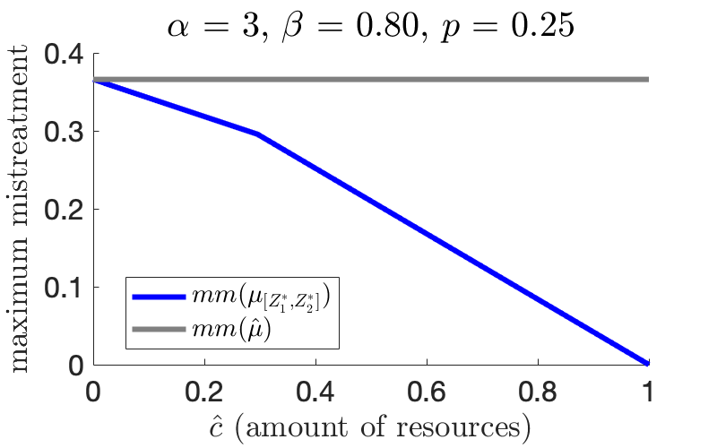
(a) Maximum mistreatment

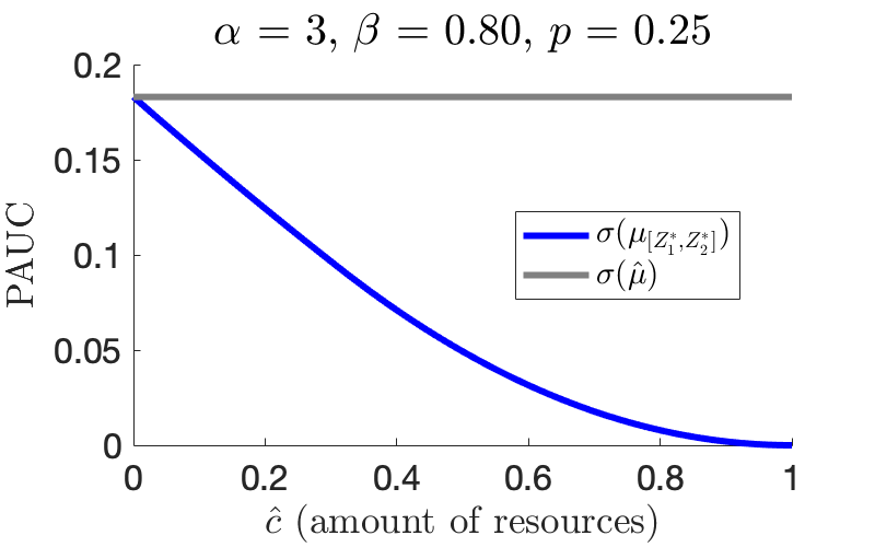
(b) PAUC

Figure 4: Effect of bias after debiasing the best set of $G_{2}$ students given $\widehat{c}$.

As we show next, the optimal set of students to target for vouchers is quite similar, whether we want to minimize the most mistreated student or the PAUC. Before stating the results formally, we need to introduce new notations. For $\widehat{c}\in[0,1]$, let $\mathcal{T}(\widehat{c})$ to be all sets $T\subseteq[1,\infty)$ such that $\int_{t\in T}dF_{1}(t)\leq\widehat{c}$. Here, $\widehat{c}$ models the amount of resources or vouchers, and each $T\in\mathcal{T}(\widehat{c})$ represents the potentials of $G_{2}$ students to whom vouchers are provided so that their true potentials will be revealed. That is, for $\theta\in G_{2}$ such that $Z(\theta)\in T$, we now have $\widehat{Z}(\theta)=Z(\theta)$ after the intervention.

Let $\mu_{T}:\Theta\rightarrow[0,1]$ be the ranking of the students after $G_{2}$ students whose real potentials lie in $T$ have been debiased. In addition, let $\mathcal{T}_{mm}(\widehat{c})$ be the collection of sets $T$ such that $\sup(\mu_{T}-\mu)$ is minimized. Next result gives an explicit characterization of those sets, assuming

$$p<1-\beta^{\alpha}.$$ (3)

This is a reasonable assumption because of the following. First, $[2,3.5]$ is a reasonable range to assume for the parameter $\alpha$ in terms of academic achievements due to Clauset et al. (2009). Then, if we, for example, assume $\alpha=3$, even with mild biases towards $G_{2}$ students, say with $\beta=.9$, we only need $p<1-.9^{3}=.271$. And with stronger bias, say $\beta=.8$, the requirement on $p$, which is $p<1-.8^{3}=.488$, is more relaxed.

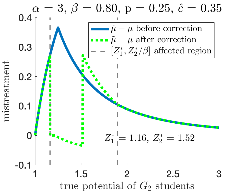
(a) optimal correction when $\widehat{c}$ is large

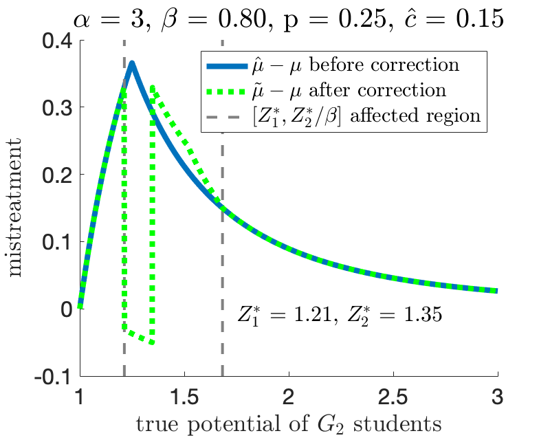
(b) optimal correction when $\widehat{c}$ is small

Figure 5: Maximum mistreatment before and after optimal voucher correction.

Theorem 4.2

Assume $p<1-\beta^{\alpha}$. Then there exists a set $T=[Z_{1}^{*},Z_{2}^{*}]\in\mathcal{T}_{mm}(\widehat{c})$ such that all other sets from $\mathcal{T}_{mm}(\widehat{c})$ differ from $T$ on a set of measure zero. If $\widehat{c}\geq\frac{(1-p)(1-\beta^{\alpha})}{1-p+1-\beta^{\alpha}}$, then

$$Z_{1}^{*}=\bigg{(}\frac{(1-p)+(\frac{1}{\beta^{\alpha}}-1)\widehat{c}}{\frac{1}{\beta^{\alpha}}-p}\bigg{)}^{-\frac{1}{\alpha}}\quad\text{and}\quad Z_{2}^{*}=\bigg{(}\frac{(1-p)(1-\widehat{c})}{\frac{1}{\beta^{\alpha}}-p}\bigg{)}^{-\frac{1}{\alpha}},$$

and $mm(\mu_{[Z_{1}^{*},Z_{2}^{*}]})=(1-p)(1-\beta^{\alpha})\frac{1-\widehat{c}}{1-p\beta^{\alpha}}$, reduced from $mm(\widehat{\mu})=(1-p)(1-\beta^{\alpha})$. Conversely, if $\widehat{c}\leq\frac{(1-p)(1-\beta^{\alpha})}{1-p+1-\beta^{\alpha}}$, then:

$$Z_{1}^{*}=\bigg{(}\frac{(1-p-\widehat{c})\beta^{\alpha}}{1-p}+\widehat{c}\bigg{)}^{-\frac{1}{\alpha}}\quad\text{ and }\quad Z_{2}^{*}=\bigg{(}\frac{(1-p-\widehat{c})\beta^{\alpha}}{1-p}\bigg{)}^{-\frac{1}{\alpha}},$$

and $mm(\mu_{[Z_{1}^{*},Z_{2}^{*}]})=(1-p-\widehat{c})(1-\beta^{\alpha})+p\widehat{c}$.

We include a proof of Theorem 4.2 in the e-companion, Section 9.2.

A pictorial representation of Theorem 4.2 is given in Figure 5. The two sub-figures correspond to two choices of $\widehat{c}$. Moreover, Figure 4(a) shows how much $mm(\mu_{[Z_{1}^{*},Z_{2}^{*}]})$ decreases as $\widehat{c}$, the amount of resources, increases. Besides minimizing the maximum of students’ mistreatment, we also investigate the objective of minimizing the aggregate amount of mistreatment received by all $G_{2}$ students (PAUC). We defer details of this analysis to Appendix 9.3, and here instead we compute optimal debiasing choices for some examples in Table 1.

Table 1 shows that, for reasonable choices of the parameters, the optimal intervals to be debiased for minimizing the maximum mistreatment and PAUC are very close. That is, the optimal intervals of potentials of students to whom vouchers should be distributed under our two measures of unfairness approximately coincide. Moreover, both measures suggest that vouchers should be given to the average (middle performing) students.

We remark that the current distribution of vouchers violates individual fairness (Dwork et al. 2012): it does not treat similar individuals similarly, as seen by individuals at the boundary of the debiasing interval. However one could get around this by randomization or distributing “partial” vouchers. This would not change the interval to be targeted, however would likely smooth out the boundaries of the interval. We leave this as an extension for future work.

$\widehat{c}$	$\mathcal{T}_{mm}(\widehat{c})=[Z_{1},Z_{2}]$	$\mathcal{T}_{auc}(\widehat{c})=[Z_{1}^{\prime},Z_{2}^{\prime}]$	$Z_{1}-Z_{1}^{\prime}$
0.10	[1.2252, 1.3111]	[1.2187, 1.3026]	0.0065
0.20	[1.2022, 1.3861]	[1.1903, 1.3653]	0.0119
0.30	[1.1802, 1.4803]	[1.1644, 1.4421]	0.0158
0.40	[1.1461, 1.5584]	[1.1346, 1.5203]	0.0115
0.50	[1.1156, 1.6560]	[1.1070, 1.6155]	0.0086
0.60	[1.0881, 1.7839]	[1.0819, 1.7403]	0.0063
0.70	[1.0632, 1.9635]	[1.0589, 1.9154]	0.0043
0.80	[1.0404, 2.2476]	[1.0377, 2.1926]	0.0026

Table 1: Compare the optimal ranges of $G_{2}$ students to debias under two measures of unfairness, under parameters $\alpha=3$, $\beta=.8$, and $p=.25$.

5 Extensions to General Distributions of Potentials

Besides Pareto distribution, our framework can also be applied to any other distributions of student potentials. For ease of notation, assume the distribution is continuous and let $f$ and $\bar{F}$ denote the pdf and ccdf of students’ true potentials respectively. In calculating the displacement of $G_{1}$ and $G_{2}$ students, similar to (1), one can compute $\widehat{\mu}(\theta)$, the school student $\theta$ actually attend due to bias in the evaluation, using

$$\widehat{\mu}(\theta)=\begin{cases}(1-p)\bar{F}(Z(\theta))+p\bar{F}(Z(\theta)/\beta)&\text{ if }\theta\in G_{1},\\[2.84526pt] (1-p)\bar{F}(\beta Z(\theta))+p\bar{F}(Z(\theta))&\text{ if }\theta\in{G_{2}};\end{cases}$$

and when $\beta=1$, we obtain $\mu(\theta)=\bar{F}(Z(\theta))$, the school student $\theta$ should attend.

In analyzing the utilities of schools, the cutoff for school $s$, $d(s)$, is the perceived potential $\widehat{z}$ such that $(1-p)\bar{F}(\widehat{z})+p\bar{F}(\widehat{z}/\beta)=s$. Thus, the utility of school $s$ under $\widehat{\mu}$ is

$$u_{\widehat{\mu}}(s)=\frac{(1-p)f(d(s))}{(1-p)f(d(s))+pf(d(s)/\beta)}\cdot d(s)+\frac{pf(d(s)/\beta)}{(1-p)f(d(s))+pf(d(s)/\beta)}\cdot\frac{d(s)}{\beta}.$$

Note that when $\beta=1$, we recover $u_{\mu}(s)=\bar{F}^{-1}(s)$.

Next, consider the two approaches of bias mitigation. We start with schools’ incentives of interviewing students. Let $\widetilde{\mu}$ denote the ranking of students when all schools decide to interview and all schools have the same interview capacity. Proposition 4.1 can be generalized as

$$u_{\widetilde{\mu}}(s)=\frac{(1-p)f(d_{1}^{i}(s))}{(1-p)f(d_{1}^{i}(s))+pf(d_{2}^{i}(s))}d_{1}^{i}(s)+\frac{pf(d_{2}^{i}(s))}{(1-p)f(d_{1}^{i}(s))+pf(d_{2}^{i}(s))}d_{2}^{i}(s),$$

where $d_{1}^{i}(s)$ and $d_{2}^{i}(s)$, the cutoffs in term of true potentials for $G_{1}$ and $G_{2}$ students respectively, follow the same formulae as those given in Proposition 4.1 with $\bar{F}_{1}$ replaced by $\bar{F}$.

For the intervention, assume $G_{2}$ students whose true potentials are within $[Z_{1},Z_{2}]$ are offered the vouchers and have their true potentials revealed, then one can compute $\widetilde{\mu}(\theta)$ for $\theta\in G_{2}$ by the following formula

$$\widetilde{\mu}(\theta)=\begin{cases}(1-p)\bar{F}(\beta Z(\theta))+p\bar{F}(Z(\theta))+p\max\big{(}0,\bar{F}(\beta Z(\theta)\vee Z_{1})-\bar{F}(Z_{2})\big{)}&\text{ if }Z(\theta)>Z_{2},\\[2.84526pt] (1-p)\bar{F}(Z(\theta))+p\big{(}\bar{F}(Z(\theta))-\bar{F}(Z_{2})\big{)}+p\bar{F}(Z(\theta)/\beta\vee Z_{2})&\text{ if }Z(\theta)\in[Z_{1},Z_{2}],\\[2.84526pt] (1-p)\bar{F}(\beta Z(\theta))+p\bar{F}(Z(\theta))&\text{ if }Z(\theta)<Z_{1}.\end{cases}$$

Although closed form solutions may not exist in general when finding the best range of $G_{2}$ students to offer vouchers under the two measures of unfairness, one can use simulations and grid search to find such best range. In Section 6.2, we present a detailed analysis in the case of normal distribution when looking at the SAT scores of New York City high school students.

6 Experimental Case Studies

In Section 6.1, we relax some of our model assumptions and empirically compare the results we obtain against the theoretical findings of the previous sections. In Section 6.2, we analyze our framework based on the SAT scores of NYC high school students, which follow a Gaussian distribution.

6.1 Empirical validation of the robustness of our conclusions

In this section, we provide an empirical investigation of the robustness of the results of the optimal set of students to target for vouchers under the PAUS measures. Those results have been discussed in Section 4.2 and are presented formally in Theorem 9.2 in the Appendix. In particular, we consider models where one or more of the following modifications are implemented: the continuous sets representing schools and students are replaced by discrete sets, with schools having finite capacities; we allow each $G_{2}$ student to a random bias factor; we assume that only a percentage of students receiving a voucher will use it (and hence be debiased). For each of those models, given a fixed set of resources $\widehat{c}$, we compare the PAUC under the theoretically optimal interval given in Theorem 9.2 and the PAUC under the optimal interval obtained numerically (by using a sliding window). Our results, discussed in detail in Appendix 10, show that, depending on the deviation from our model, the predictions from Theorem 9.2 stay between close to and very close to the optimum, and in all cases provide a very significant improvement over the status quo.

Intervention Range		PAUC		Maximum Mistreatment
$\emptyset$		0.4238		0.3216
$[-\infty,1387]$		0.3022		0.2415
$[1229,1511]$		0.2934		0.3165
$[1387,1629]$		0.2645		0.3619
$[1511,1759]$		0.2228		0.3644
$[1695,2187]$		0.1658		0.2302
$[1700,2231]$		0.1657		0.2078
$[1713,\infty]$		0.1684		0.2095

Table 2: PAUC and maximum mistreatment under different intervention range.

6.2 NYC High Schools SAT Scores

Prior to March 2016, the SAT exam had three sections: mathematics, critical reading, and writing. Each section is reported on a scale from 200 to 800. Although not exclusively, students’ performance on the SAT exam is one of the factors considered by the college admission team. Due to the universality of SAT scores, we will use SAT scores as a proxy for high school students’ potentials. Moreover, since SAT scores follows a normal distribution, we can use data on SAT scores to study our model empirically when the distribution of students’ potentials are assumed to be Gaussian.

The primary dataset we use is compiled by NYC Open Data and downloaded from Kaggle (2015). The dataset contains information regarding high schools in New York City during the 2014–2015 academic year, including the average SAT score of each school, the number of SAT test takers from each school. To simulate and mimic the SAT scores of high school students in New York City, we further use distribution information, standard deviation to be specific, of SAT scores from a report published by College Board (2016). In particular, for each test taker of a given high school, his or her SAT score is drawn randomly from a normal distribution with mean being the reported school average and standard deviation obtained from the College Board report. Since SAT scores cannot be lower than 600, nor higher than 2400, we truncated those simulated scores which are outside the standard range.

In order to distinguish between $G_{1}$ students and $G_{2}$ students, we make use of another dataset from NYC Open Data (2017), that contain the Economic Need of each school. Details are presented in Appendix 11.1. We already discussed in Section 1.1 how Figure 1(a) allows us to estimate a bias factor of $\beta=.8$ for this dataset. In addition, we assume students’ true potentials follow a normal distribution with mean 1,550 and standard deviation 310. The mean and standard deviation are estimated from the simulated data. Results on the displacement of students, impact of bias on schools utilities, and interview processes are similar to the case of the Pareto distribution, and presented in detail in Appendix 11.2.

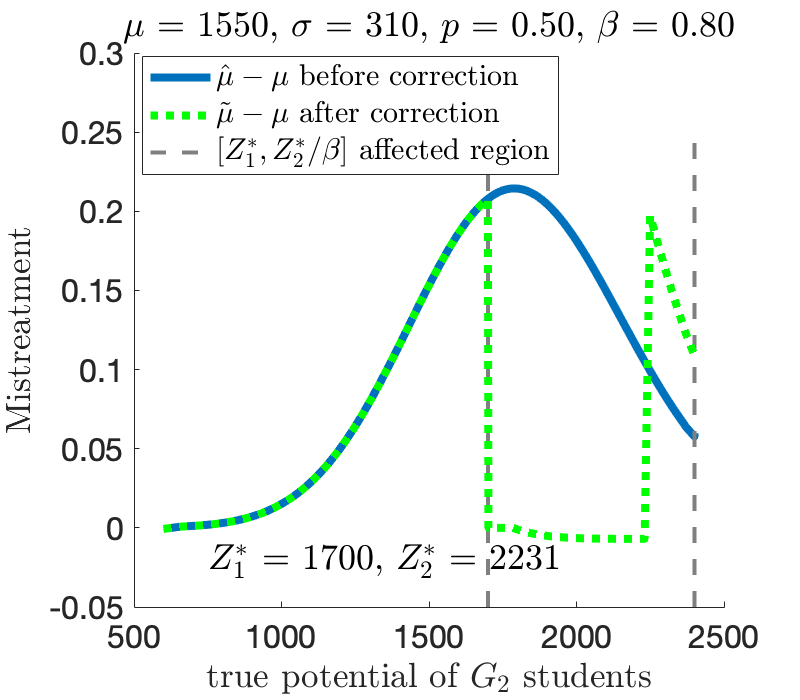
Figure 23: Best intervention strategy.

In terms of intervention, using grid search, for each of the two measures of unfairness (recall, most significant mistreatment and average mistreatment), we can obtain the empirically optimal interval of potentials of $G_{2}$ students to debias. Assume the amount of vouchers $\widehat{c}=0.30$, the resulting two measures of unfairness under different debiasing intervals are summarized in Table 2. The first row of the table is the baseline when no intervention measure is taken. The best interval under the two measures of unfairness coincide for the experimented setting (although in general, we do not expect this to be true). In particular, vouchers should be offered to the middle top students. The mistreatment of $G_{2}$ students before and after intervention on the empirically optimal interval $G_{2}$ students is illustrated in Figure 23 in the Appendix.

Omitted Proofs

7 Discussion on discrete versus continuous models for two-sided matching markets

Traditionally, matching markets are assumed to be discrete (Gale and Shapley 1962, Roth and Sotomayor 1992). There has been however, in recent years, an interest for models where one or both sides of the markets are continuous (Arnosti 2019, Azevedo and Leshno 2016). This is justified by the fact that, in many applications, markets are large, hence predictions in continuous markets often translate with a good degree of accuracy to discrete ones. Moreover, continuous markets are often analytically more tractable than discrete ones (see, again, Arnosti (2019), Azevedo and Leshno (2016)). Our case is no exception: the continuous model allows us to deduce precise mathematical formulae, while we show through experiments that those formulae are a good approximation to the discrete case. We also provide additional experiments evaluating the robustness of our results under relaxation of assumptions, such as that of a unique bias factor for all students in $G_{2}$. We remark that the goal of this study is not to provide a mechanism to admits students to schools, for which the assumption of all rankings of schools as well as of students being the same would be too simplistic. On the contrary, as we want to understand the impact of bias at a macroscopic level, we believe our approximation to be meaningful and useful since as in our model any reasonable mechanism would output the same assignment.

8 Additional details from Section 3

8.1 Additional figure on the results from Section 3.1

The displacement function is plotted for one set of parameters in Figure 6.

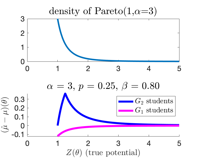
Figure 6: Pareto Density and Displacements of students

8.2 Proof of Proposition 3.2

In order for a student $\theta$ to be assigned to a school that is at least as good as $s$, his or her perceived potential $\widehat{Z}(\theta)$ needs to be high enough to satisfy $(1-p)\bar{F}_{1}(1\vee\widehat{Z}(\theta))+p\bar{F}_{2}(\widehat{Z}(\theta))\leq s$. That is, we need

$$\widehat{Z}(\theta)\geq d(s):=\begin{cases}\displaystyle\left(\frac{s}{1-p+p\beta^{\alpha}}\right)^{-\frac{1}{\alpha}}&\text{if }s\leq 1-p+p\beta^{\alpha},\\[2.84526pt] \displaystyle\beta\left(\frac{s-(1-p)}{p}\right)^{-\frac{1}{\alpha}}&\text{if }s>1-p+p\beta^{\alpha}.\end{cases}$$

We call $d(s)$ the cutoff for school $s$. With the cutoffs, we can compute the utilities of schools. We start with the formula for $u_{\widehat{\mu}}(s)$. First note that by Bayes rule, the probability that a given student with perceived potential $\widehat{Z}(\theta)\geq 1$ belongs to $G_{1}$ is $\frac{1-p}{1-p+p\beta^{\alpha+1}}$. Using (1), observe that the $G_{2}$ student whose perceived potential is $1$ (i.e., true potential is $\frac{1}{\beta}$) is matched to school $1-p+p\beta^{\alpha}$. Thus, if $s\geq 1-p+p\beta^{\alpha}$, $s$ is only assigned with $G_{2}$ students. Therefore, when $s\leq 1-p+p\beta^{\alpha}$,

$$u_{\widehat{\mu}}(s)=\frac{1-p}{1-p+p\beta^{\alpha+1}}d(s)+\frac{p\beta^{\alpha+1}}{1-p+p\beta^{\alpha+1}}\frac{d(s)}{\beta}=\frac{1-p+p\beta^{\alpha}}{1-p+p\beta^{\alpha+1}}\left(\frac{s}{1-p+p\beta^{\alpha}}\right)^{-\frac{1}{\alpha}}.$$

And when $s>1-p+p\beta^{\alpha}$, we have

$$u_{\widehat{\mu}}(s)=d(s)/\beta=\left(\frac{s-(1-p)}{p}\right)^{-\frac{1}{\alpha}}.$$

One the other hand, when there is no bias against $G_{2}$ students, we simply have $u_{\mu}(s)=s^{-\frac{1}{\alpha}}$.

8.3 Diversity in schools

We now investigate how bias affects diversity in schools. Let $pr(s)$ (resp. $\widehat{pr}(s)$) be the proportion of $G_{2}$ students assigned to school $s$ when there is no bias (resp. there is bias) against $G_{2}$ students.

Proposition 8.1

Without bias, we have $pr(s)=p$. Under the biased setting, we have

$$\widehat{pr}(s)=\begin{cases}\displaystyle\frac{p\beta^{\alpha}}{1-p+p\beta^{\alpha}}&\text{ if }s\leq 1-p+p\beta^{\alpha},\\ 1&\text{ if }s>1-p+p\beta^{\alpha}.\end{cases}$$

Proof 8.2

The claim $pr(s)=p$ for all $s\in[0,1]$ follows from the fact that the distribution of true potentials is the same for $G_{1}$ and $G_{2}$ students. The formula for $\widehat{pr}(s)$ follows from the discussion in proof of Proposition 3.2.

A visual comparison of $pr(s)$ and $\widehat{pr}(s)$ can be found in Figure 7 for different values of $\beta$ and $p$.

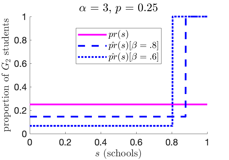
Figure 7: Proportion of $G_{2}$ students in higher ranked schools decreases significantly in the biased setting.

9 Additional details from Section 4

9.1 Proof of Proposition 4.1

By Bayes rule, we have that for school $s$, its proportion of $G_{1}$ students is

$$\frac{(1-p)[d_{1}^{i}(s)]^{-(\alpha+1)}}{(1-p)[d_{1}^{i}(s)]^{-(\alpha+1)}+p[d_{2}^{i}(s)]^{-(\alpha+1)}}.$$

Hence, the formula for $u_{\widetilde{\mu}}(s)$ when $d_{1}^{i}(s)>1$ follows from the same arguments given in the proof of Proposition 3.2. When $d_{1}^{i}(s)=1$, only $G_{2}$ students are assigned to $s$ and thus, $u_{\widetilde{\mu}}(s)=d_{2}^{i}(s)$.

Now, for the cutoffs, consider a fixed school $s$. Under the continuous model, the amount of students school $s$ is matched to has Lebesgue measure $0$, so it is more useful to think of the cutoffs in terms of all the schools that are at least as good as $s$. If $\bar{F}_{1}\big{(}d(\min(1,s+iv))/\beta\big{)}\geq s$, that is, if all schools that are as least as good as $s$ interview more $G_{2}$ students than they are willing to admit, then the cutoffs for $G_{1}$ and $G_{2}$ students are the same. On the other hand, if $\bar{F}_{1}\big{(}d(\min(1,s+iv))/\beta\big{)}<s$, then schools that are at least as good as $s$ do not interview enough $G_{2}$ students and as a result, they admit all the $G_{2}$ interviewees, and fill in the rest with $G_{1}$ students. This gives rise to the formulae for cutoffs $d_{1}^{i}(s)$ and $d_{2}^{i}(s)$.

9.2 Proof of Theorem 4.2 and related facts

9.2.1 Technical discussion

The main idea of the proof is to first assume that the set $T$ forms a connected set (i.e., a closed interval). Then, we can express $mm(\mu_{T})$ as a function of the endpoints of $T$ and work out the minimizing interval. We next drop the assumption that $T$ is connected and show that the optimal set of students to debias remains the same. The analysis we give is actually more general, and presents results under which vouchers improve the mistreatment of students lexicographically. Interestingly, it also shows that, if vouchers are not distributed carefully, one may actually worsen the most mistreated students.

9.2.2 A more general approach

The analysis we give is actually more general, and has the goal of investigating conditions under which giving vouchers can improve over the status quo. More formally, for bounded functions $f,g:G_{2}\rightarrow\mathbb{R}$, we write $f\succ g$ if we can partition $G_{2}$ in two sets $S,S^{\prime}$ (with possibly $S^{\prime}=\emptyset$) so that $f(\theta)=g(\theta)$ for $\theta\in S^{\prime}$ and $\sup_{\theta\in S}f(\theta)>\sup_{\theta\in S}g(\theta)$. Note that $\succ$ is transitive and antisymmetric, and can be interpreted as a continuous equivalent of the classical lexicographic ordering for discrete vectors. In particular, if we let $f=\gamma-\mu$ and $g=\gamma^{\prime}-\mu$ for matchings $\gamma,\gamma^{\prime}$, then $\sup_{\theta\in G_{2}}(\gamma-\mu)(\theta)>\sup_{\theta\in G_{2}}(\gamma^{\prime}-\mu)(\theta)$ implies $f\succ g$ (taking $S=G_{2}$). Now suppose we debias student in $T=[Z_{1},Z_{2}]$ for some $T\in\mathcal{T}(\widehat{c})$, and let $f:=\widehat{\mu}-\mu$, $g:=\mu_{T}-\mu$. Table 3 provides conditions under which $f\succ g$ (i.e., intervention reduces the maximum mistreated experienced by $G_{2}$ students). In particular it shows that for certain combinations of the data and the choice of $Z_{1}$ and $Z_{2}$, giving vouchers may actually lead to worse (according to $\succ$) matchings. One can check that under assumption (3), all conditions given in Table 3 for different cases are satisfied.

CASE	subcase	condition for $\widehat{\mu}-\mu\succ\mu_{T}-\mu$
I. $\beta Z_{2}\geq Z_{1}$	1. $1\leq\beta Z_{1}$	$\displaystyle p<1-\left(\frac{Z_{1}}{Z_{2}}\right)^{\alpha}$
	2. $\beta Z_{1}\leq 1\leq\beta Z_{2}$	$\displaystyle p<1-\left(\frac{1}{\beta Z_{2}}\right)^{\alpha}$
II. $\beta Z_{2}\leq Z_{1}$	1. $1\leq\beta Z_{1}$	$\displaystyle p<1-\beta^{\alpha}$
	2. $\beta Z_{1}\leq 1\leq\beta Z_{2}$	$\displaystyle p\left(\left(\frac{1}{Z_{1}}\right)^{\alpha}-\left(\frac{1}{Z_{2}}\right)^{\alpha}\right)<(1-p)\left(\frac{1}{\beta^{\alpha}}-1\right)\left(\beta^{\alpha}-\left(\frac{1}{Z_{2}}\right)^{\alpha}\right)$
	3. $\beta Z_{2}\leq 1$	Not possible: $g\succ f$ in this case.

Table 3: Sufficient conditions for $\widehat{\mu}-\mu\succ\mu_{T}-\mu$ by cases, where $T=[Z_{1},Z_{2}]$. Each strict inequality, when replaced with its non-strict counterpart, gives instead a necessary condition.

In this first part of the proof, we proceed as follows. First, we assume that $T\in\mathcal{T}^{c}(\widehat{c})$. That is, we assume $T=[Z_{1},Z_{2}]$ with extreme points $Z_{1}<Z_{2}$. For simplicity, we let $\widetilde{\mu}$ denote $\mu_{T}$. We then compare $f:=\widehat{\mu}-\mu$ and $g:=\widetilde{\mu}-\mu$ using the relation $\succ$.

Note that, if we let $S$ be the set of students in $G_{2}$ with potential in $[Z_{1},Z_{2}/\beta]$ and $S^{\prime}:=G_{2}\setminus S$, we have $f(\theta)=g(\theta)$ for $\theta\in S^{\prime}$. That is, only $G_{2}$ students whose true potential lies in interval $[Z_{1},Z_{2}/\beta]$ are affected by the intervention. Hence, $\sup_{\theta\in S}f>\sup_{\theta\in S}g$ if and only if $f\succ g$.

We divide the analysis in the following two major cases: the first case is when $\beta Z_{2}\geq Z_{1}$ (i.e., when $[\beta Z_{1},\beta Z_{2}]$ and $[Z_{1},Z_{2}]$ overlap) and the second case is when $\beta Z_{2}\leq Z_{1}$. For both major cases, we will consider two subcases: $\beta Z_{1}\geq 1$, $\beta Z_{1}\leq 1\leq\beta Z_{2}$. And for the second major case, we also need to consider the subcase where $\beta Z_{2}\leq 1$. The results for all cases are summarized in the Table 3.

9.2.3 CASE I: $\beta Z_{2}\geq Z_{1}$

The dashed lines represent perceived potential equaling to $1$, and the two dashed lines represent the two subcases we will consider.

Subcase 1. $1\leq\beta Z_{1}$. Under the status quo $\widehat{\mu}$, the student in $S$ that is most unfairly treated is the one whose true potential is $Z_{1}$. This can be easily observed from Figure 6. Thus,

$$\sup_{\theta\in S}\{(\widehat{\mu}-\mu)(\theta)\}=(1-p)\left(\frac{1}{Z_{1}}\right)^{\alpha}\left(\frac{1}{\beta^{\alpha}}-1\right).$$ (4)

Now, for the ranking $\widetilde{\mu}$ after voucher correction, $G_{2}$ students whose true potentials are within $[Z_{1},Z_{2}]$ (i.e., those whose true potentials are revealed through vouchers) are not harmed under $\widetilde{\mu}$. That is, for all $G_{2}$ student $\theta$ such that $Z(\theta)\in[Z_{1},Z_{2}]$, we have $(\widetilde{\mu}-\mu)(\theta)\leq 0$, with equality achieved for $G_{2}$ students whose true potentials are in $[Z_{1},\beta Z_{2}]$. Thus, the $G_{2}$ student who experience the maximum mistreatment must have potential in the interval $[Z_{2},Z_{2}/\beta]$. In particular, for every $G_{2}$ student $\theta\in S$, we have

$$\widetilde{\mu}(\theta) =p\bar{F}_{2}(\beta Z(\theta))+(1-p)\bar{F}_{1}(\beta Z(\theta))+p(\bar{F}_{2}(\beta^{2}Z(\theta))-\bar{F}_{2}(\beta Z_{2})),$$

where the three components correspond to $G_{2}$ students with better perceived potentials even before the intervention, $G_{1}$ students with better perceived potentials, and additional $G_{2}$ students with better perceived potentials after after the intervention. Thus, for $\theta\in S$,

$$(\widetilde{\mu}-\mu)(\theta) =p\left(\frac{1}{Z(\theta)}\right)^{\alpha}+(1-p)\left(\frac{1}{\beta Z(\theta)}\right)^{\alpha}+p\left(\left(\frac{1}{\beta Z(\theta)}\right)^{\alpha}-\left(\frac{1}{Z_{2}}\right)^{\alpha}\right)-\left(\frac{1}{Z(\theta)}\right)^{\alpha}$$

$$=\left(\frac{1}{Z(\theta)}\right)^{\alpha}\underbrace{\left(p+\frac{1}{\beta^{\alpha}}-1\right)}_{>0}-p\left(\frac{1}{Z_{2}}\right)^{\alpha}.$$

Thus, the supremum is achieved for $\bar{\theta}\in G_{2}$ such that $Z(\bar{\theta})=Z_{2}$. That is,

$$\sup_{\theta\in S}\{(\widetilde{\mu}-\mu)(\theta)\}=(\widetilde{\mu}-\mu)(\bar{\theta})=\left(\frac{1}{\beta^{\alpha}}-1\right)\left(\frac{1}{Z_{2}}\right)^{\alpha},$$ (5)

and $f\succ g$ if

$$(1-p)\left(\frac{1}{Z_{1}}\right)^{\alpha}\left(\frac{1}{\beta^{\alpha}}-1\right)>\left(\frac{1}{\beta^{\alpha}}-1\right)\left(\frac{1}{Z_{2}}\right)^{\alpha}\Leftrightarrow p<1-\left(\frac{Z_{1}}{Z_{2}}\right)^{\alpha}.$$

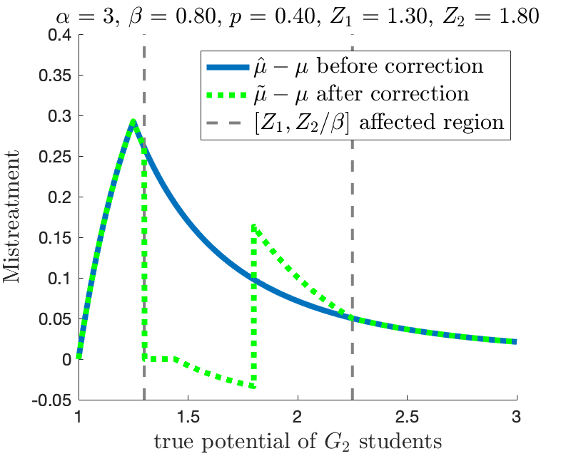
(a) when correction is better in the affected region

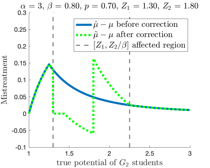
(b) when correction is worse in the affected region

Figure 8: Mistreatment of $G_{2}$ student before and after voucher correction for CASE I-1.

See Figure 8 for a comparison of $\widetilde{\mu}-\mu$ and $\widehat{\mu}-\mu$ under this subcase. Two subfigures have different values of $p$. When $p=0.40$ (left), voucher correction decreases the maximum mistreatment (i.e., $f\succ g$). However, when $p=0.70$ (right), voucher correction actually increases the maximum mistreatment experienced by $G_{2}$ students (i.e., $g\succ f$).

Subcase 2. $\beta Z_{1}\leq 1\leq\beta Z_{2}$. Before the correction, the $G_{2}$ student that is mistreated the most is the one whose perceived potential is $1$ (i.e., true potential is $1/\beta$). That is,

$$\sup_{\theta\in S}\{(\widehat{\mu}-\mu)(\theta)\}=(\widehat{\mu}-\mu)\left(\frac{1}{\beta}\right)=(1-p)\left(1-\beta^{\alpha}\right).$$ (6)

Note that $Z_{1}\geq 1$ since $Z_{1}$ denotes the true potential. Thus, it is not hard to see that the previous analysis remains valid. In particular, equation (5) holds. Therefore, $f\succ g$ if

$$(1-p)(1-\beta^{\alpha})>\left(\frac{1}{\beta^{\alpha}}-1\right)\left(\frac{1}{Z_{2}}\right)^{\alpha}\Leftrightarrow p<1-\left(\frac{1}{\beta Z_{2}}\right)^{\alpha}.$$

See Figure 9 for a demonstration of scenarios under this case. Similarly, two subfigures are presented, one for when $f\succ g$ and one for when $g\succ f$.

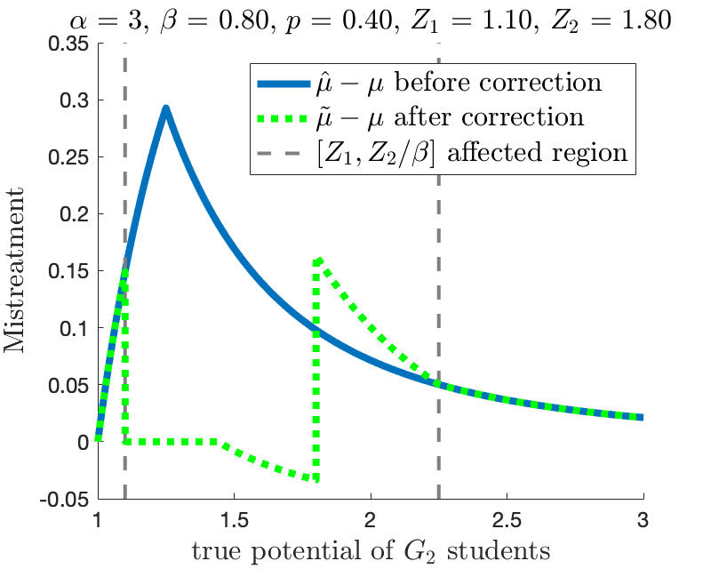
(a) when correction is better in the affected region

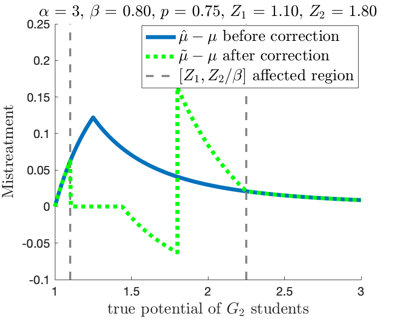
(b) when correction is worse in the affected region

Figure 9: Mistreatment of $G_{2}$ student before and after voucher correction for CASE I-2.

9.2.4 CASE II: $\beta Z_{2}\leq Z_{1}$

As in the previous case, the dashed lines represent perceived potential equaling to $1$, and three dashed lines represent the three different subcases we will consider. Note that besides the two cases in the previous case, we also have a third additional case to consider.

Subcase 1. $1\leq\beta Z_{1}$. Equation (4) holds for $\widehat{\mu}-\mu$. And as for the matching $\widetilde{\mu}$ after voucher correction, with the same argument, it is clear that $\sup_{\theta\in S}\{(\widetilde{\mu}-\mu)(\theta)\}$ is achieved for some $\theta\in G_{2}$ with $Z(\theta)\in[Z_{2},Z_{2}/\beta]$. However, to have a complete analysis, we need to consider the following two ranges, $[Z_{2},Z_{1}/\beta]$ and $[Z_{1}/\beta,Z_{2}/\beta]$, separately as the expressions for $\widetilde{\mu}(\theta)$ differ.

First Range $[Z_{1}/\beta,Z_{2}/\beta]$. Here, $\widetilde{\mu}$ has the same expression as in case I.1 and thus the supremum of $\widetilde{\mu}-\mu$ in this range is achieved at $\bar{\theta}\in S$ such that $Z(\bar{\theta})=Z_{1}/\beta$.

$$\sup_{\theta\in S:Z(\theta)\in[Z_{1}/\beta,Z_{2}/\beta]}\{(\widetilde{\mu}-\mu)(\theta)\}=(\widetilde{\mu}-\mu)(\bar{\theta}).$$

Second Range $[Z_{2},Z_{1}/\beta]$. In this range, we have

$$\widetilde{\mu}(\theta)=p\bar{F}_{2}(\beta Z(\theta))+(1-p)\bar{F}_{1}(\beta Z(\theta))+p\big{(}\bar{F}_{2}(Z_{1})-\bar{F}_{2}(Z_{2})\big{)}$$

and

$$(\widetilde{\mu}-\mu)(\theta) =p\left(\frac{1}{Z(\theta)}\right)^{\alpha}+(1-p)\left(\frac{1}{\beta Z(\theta)}\right)^{\alpha}+p\left(\left(\frac{1}{Z_{1}}\right)^{\alpha}-\left(\frac{1}{Z_{2}}\right)^{\alpha}\right)-\left(\frac{1}{Z(\theta)}\right)^{\alpha}$$

$$=\left(\frac{1}{Z(\theta)}\right)^{\alpha}\underbrace{(1-p)\left(\frac{1}{\beta^{\alpha}}-1\right)}_{>0}+p\left(\left(\frac{1}{Z_{1}}\right)^{\alpha}-\left(\frac{1}{Z_{2}}\right)^{\alpha}\right).$$

Thus, the supremum of $\widetilde{\mu}-\mu$ in this range is achieved at $\underline{\theta}\in S$ such that $Z(\underline{\theta})=Z_{2}$.

$$\sup_{\theta\in S:Z(\theta)\in[Z_{2},Z_{1}/\beta]}\{(\widetilde{\mu}-\mu)(\theta)\}=(\widetilde{\mu}-\mu)(\underline{\theta}).$$

All together, since $\widetilde{\mu}-\mu$ is continuous, we have

$$\sup_{\theta\in S}\{(\widetilde{\mu}-\mu)(\theta)\}=(\widetilde{\mu}-\mu)(\underline{\theta})=p\left(\frac{1}{Z_{1}}\right)^{\alpha}+\left(\frac{1}{Z_{2}}\right)^{\alpha}\left((1-p)\frac{1}{\beta^{\alpha}}-1\right),$$ (7)

and thus, $f\succ g$ if

$$(1-p)\left(\frac{1}{Z_{1}}\right)^{\alpha}\left(\frac{1}{\beta^{\alpha}}-1\right)>p\left(\frac{1}{Z_{1}}\right)^{\alpha}+\left(\frac{1}{Z_{2}}\right)^{\alpha}\left((1-p)\frac{1}{\beta^{\alpha}}-1\right)\Leftrightarrow p<1-\beta^{\alpha}.$$

Voucher correction under this cases is shown in Figure 10.

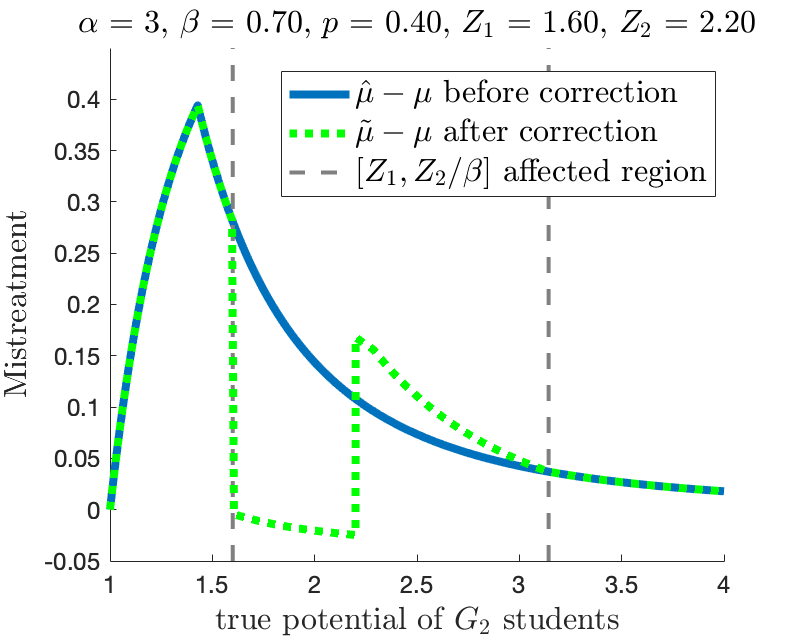
(a) when correction is better in the affected region

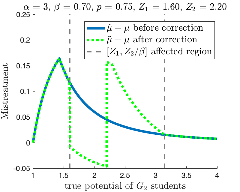
(b) when correction is worse in the affected region

Figure 10: Mistreatment of $G_{2}$ student before and after voucher correction for CASE II-1.

Subcase 2. $\beta Z_{1}\leq 1\leq\beta Z_{2}$. As in case II.2, Equation (6) holds. The analysis for $\widetilde{\mu}-\mu$ is the same as in the previous section and equation (7) is valid. Thus, $f\succ g$ if

$$(1-p)\left(\frac{1}{Z_{1}}\right)^{\alpha}\left(\frac{1}{\beta^{\alpha}}-1\right) >p\left(\frac{1}{Z_{1}}\right)^{\alpha}+\left(\frac{1}{Z_{2}}\right)^{\alpha}\left((1-p)\frac{1}{\beta^{\alpha}}-1\right)$$

$$\Leftrightarrow$$

$$p\left(\left(\frac{1}{Z_{1}}\right)^{\alpha}-\left(\frac{1}{Z_{2}}\right)^{\alpha}\right) <(1-p)\left(\frac{1}{\beta^{\alpha}}-1\right)\left(\beta^{\alpha}-\left(\frac{1}{Z_{2}}\right)^{\alpha}\right).$$

See Figure 11 for a demonstration of this subcase.

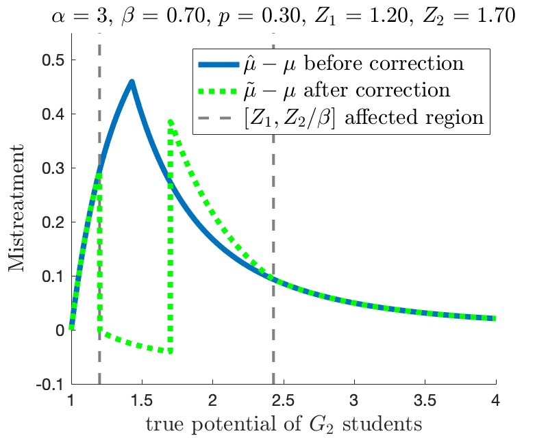
(a) when correction is better in the affected region

(b) when correction is worse in the affected region

Figure 11: Mistreatment of $G_{2}$ student before and after voucher correction for CASE II-2.

Subcase 3. $\beta Z_{2}\leq 1$. Again, we can refer to Equation (6) for $\sup_{\theta\in S}\{(\widehat{\mu}-\mu)(\theta)\}$. For voucher correction, as in case II.1, $\sup_{\theta\in S}\{(\widetilde{\mu}-\mu)(\theta)\}$ is obtained for some $\theta$ with $Z(\theta)\in[Z_{2},Z_{2}/\beta]$. To have a complete analysis, we consider three ranges, $[Z_{2},1/\beta]$, $[1/\beta,Z_{1}/\beta]$ and $[Z_{1}/\beta,Z_{2}/\beta]$, separately as the expressions for $\widetilde{\mu}$ differ, the same reason as before.

First Range $[Z_{1}/\beta,Z_{2}/\beta]$. In this range, $\widetilde{\mu}$ has the same expression as in case I.1. Thus, the supremum of $\widetilde{\mu}-\mu$ in this range is achieved at $\bar{\theta}\in S$ such that $Z(\bar{\theta})=Z_{1}/\beta$. That is,

$$\sup_{\theta\in S:Z(\theta)\in[Z_{1}/\beta,Z_{2}/\beta]}\{(\widetilde{\mu}-\mu)(\theta)\}=(\widetilde{\mu}-\mu)(\bar{\theta}).$$

Second Range $[1/\beta,Z_{1}/\beta]$. The analysis here is the same as that of the second range in Case II.1. Therefore, the supremum of $\widetilde{\mu}-\mu$ in this range is achieved at $\underline{\theta}\in S$ such that $Z(\underline{\theta})=1/\beta$. That is,

$$\sup_{\theta\in S:Z(\theta)\in[1/\beta,Z_{1}/\beta]}\{(\widetilde{\mu}-\mu)(\theta)\}=(\widetilde{\mu}-\mu)(\underline{\theta}).$$

Third Range $[Z_{2},1/\beta]$. Lastly, for this range, we have

$$\widetilde{\mu}(\theta)=p\bar{F}_{2}(\beta Z(\theta))+(1-p)+p\big{(}\bar{F}_{2}(Z_{1})-\bar{F}_{2}(Z_{2})\big{)}$$

and

$$(\widetilde{\mu}-\mu)(\theta) =p\left(\frac{1}{Z(\theta)}\right)^{\alpha}+(1-p)+p\left(\left(\frac{1}{Z_{1}}\right)^{\alpha}-\left(\frac{1}{Z_{2}}\right)^{\alpha}\right)-\left(\frac{1}{Z(\theta)}\right)^{\alpha}$$

$$=\left(\frac{1}{Z(\theta)}\right)^{\alpha}\underbrace{(p-1)}_{<0}+(1-p)+p\left(\left(\frac{1}{Z_{1}}\right)^{\alpha}-\left(\frac{1}{Z_{2}}\right)^{\alpha}\right)$$

Thus,

$$\sup_{\theta\in S:Z(\theta)\in[Z_{2},1/\beta]}\{(\widetilde{\mu}-\mu)(\theta)\}=(\widetilde{\mu}-\mu)(\underline{\theta}).$$

All together, by continuity of $\widetilde{\mu}-\mu$, we have

$$\sup_{\theta\in S}\{(\widetilde{\mu}-\mu)(\theta)\}=(\widetilde{\mu}-\mu)(\underline{\theta})=(1-p)(1-\beta^{\alpha})+p\left(\left(\frac{1}{Z_{1}}\right)^{\alpha}-\left(\frac{1}{Z_{2}}\right)^{\alpha}\right)$$

Hence, $f\succ g$ only if

$$(1-p)(1-\beta^{\alpha})\geq(1-p)(1-\beta^{\alpha})+p\left(\left(\frac{1}{Z_{1}}\right)^{\alpha}-\left(\frac{1}{Z_{2}}\right)^{\alpha}\right).$$

However, this is impossible since $Z_{1}<Z_{2}$. Hence, we always have $g\succ f$ in this case, as shown in Figure 12 with two different values of $p$.

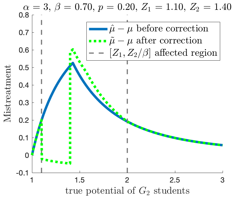
(a) correction is worse in affected region w/ small $p$

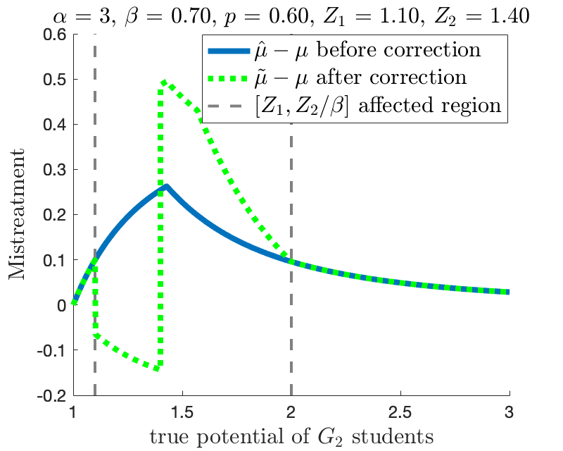
(b) correction is worse in affected region w/ large $p$

Figure 12: Mistreatment of $G_{2}$ student before and after voucher correction for CASE II-3.

9.2.5 Computing the optimal range for vouchers

We now prove Theorem 4.2 under the additional restriction that sets in $\mathcal{T}(\widehat{c})$ are connected, i.e., of the form $[Z_{1},Z_{2}]$ (we shall show later that this condition can be relaxed).

Observation 9.1

If there is an interval $[Z_{1},Z_{2}]$ that is of either case I.2 or case II.2 such that $\mu_{[Z_{1},Z_{2}]}-\mu\prec\widehat{\mu}-\mu$ with $S=G_{2}$, then the optimal range must be of case I.2 or case II.2. This is because for any interval $[Z_{1}^{\prime},Z_{2}^{\prime}]$ that is not of case I.2 or case II.2, we have

$$\sup_{\theta\in\Theta}\{(\mu_{[Z_{1}^{\prime},Z_{2}^{\prime}]}-\mu)\}\geq\sup_{\theta\in\Theta}\{\widehat{\mu}-\mu\}>\sup_{\theta\in\Theta}\{\mu_{[Z_{1},Z_{2}]}-\mu\}.$$

As it turns out, indeed, the optimal range will be either case I.2 or case II.2, and exactly which one the optimal solution is depends on the amount of resources, i.e., the magnitude of $\widehat{c}$.

We now show the first half of Theorem 4.2, i.e., we assume $\widehat{c}\geq\frac{(1-p)(1-\beta^{\alpha})}{1-p+1-\beta^{\alpha}}$. We proceed as follows:

• We first show that $[Z_{1}^{*},Z_{2}^{*}]$ is of case I.2. That is, we show $\beta Z_{2}^{*}\geq Z_{1}^{*}$ and $Z_{1}^{*}\leq\frac{1}{\beta}\leq Z_{2}^{*}$.

From the analysis in Section 9.2.3 and Section 9.2.4, one can see that for an interval $[Z_{1},Z_{2}]$ of case I.2 or case II.2, $\mu_{[Z_{1},Z_{2}]}-\mu$ increases on $[1,Z_{1}]$, deceases on $[Z_{2},\infty]$, and it is non-positive on $[Z_{1},Z_{2}]$. This means $\sup_{\theta\in\Theta}\{\mu_{[Z_{1},Z_{2}]}-\mu\}$ is achieved either at $Z_{1}$ or $Z_{2}$.

• Next, we show that $[Z_{1}^{*},Z_{2}^{*}]$ is an exact range, that is, $(\frac{1}{Z_{1}^{*}})^{\alpha}-(\frac{1}{Z_{2}^{*}})^{\alpha}=\widehat{c}$. Moreover, let $\theta_{1}^{*}$ and $\theta_{2}^{*}$ be the $G_{2}$ students whose potentials are $Z_{1}^{*}$ and $Z_{2}^{*}$ respectively. Then, $(\mu_{[Z_{1},Z_{2}]}-\mu)(\theta_{1}^{*})=(\mu_{[Z_{1},Z_{2}]}-\mu)(\theta_{2}^{*})$ and therefore, they are both equal to $\sup_{\theta\in\Theta}\{\mu_{[Z_{1},Z_{2}]}-\mu\}$.

Together with assumption (3), we have $\sup_{\theta\in\Theta}\{\mu_{[Z_{1}^{*},Z_{2}^{*}]}-\mu\}\leq\sup_{\theta\in\Theta}\{\widehat{\mu}-\mu\}$. Thus, due to Observation 9.1, it is sufficient to compare $[Z_{1}^{*},Z_{2}^{*}]$ only with intervals $[Z_{1},Z_{2}]$ of case I.2 and case II.2 (i.e, when $\beta Z_{1}\leq 1\leq\beta Z_{2}$). Since $[Z_{1}^{*},Z_{2}^{*}]$ is exact, we must either have $Z_{1}>Z_{1}^{*}$ or $Z_{2}<Z_{2}^{*}$.

• Lastly, we show that for any other feasible range $[Z_{1},Z_{2}]$ of case I.2 or case II.2, we must have $\sup_{\theta\in\Theta}\{\mu_{[Z_{1},Z_{2}]}-\mu\}>\sup_{\theta\in\Theta}\{\mu_{[Z_{1}^{*},Z_{2}^{*}]}-\mu\}$. Let $\theta_{1}$ and $\theta_{2}$ be the $G_{2}$ students whose potentials are $Z_{1}$ and $Z_{2}$. It suffices to show

  1. if $Z_{1}>Z_{1}^{*}$, then $(\mu_{[Z_{1},Z_{2}]}-\mu)(\theta_{1})>(\mu_{[Z_{1}^{*},Z_{2}^{*}]}-\mu)(\theta_{1}^{*})$;

  2. if $Z_{2}<Z_{2}^{*}$, then $(\mu_{[Z_{1},Z_{2}]}-\mu)(\theta_{2})>(\mu_{[Z_{1}^{*},Z_{2}^{*}]}-\mu)(\theta_{2}^{*})$.

STEP (1). We start by showing $\beta Z_{2}^{*}\geq Z_{1}^{*}$ through a sequence of equivalence relations:

$$\beta Z_{2}^{*}\geq Z_{1}^{*} \Leftrightarrow\left(\frac{1}{\beta Z_{2}^{*}}\right)^{\alpha}\leq\left(\frac{1}{Z_{1}^{*}}\right)^{\alpha}$$

$$\Leftrightarrow\frac{1}{\beta^{\alpha}}(1-p)(1-\widehat{c})\leq(1-p)+\left(\frac{1}{\beta^{\alpha}}-1\right)\widehat{c}$$

$$\Leftrightarrow\widehat{c}(1-\beta^{\alpha}+1-p)\geq(1-p)(1-\beta^{\alpha}).$$

Note that the last inequality is implied by the condition we have on $\widehat{c}$. We next show $Z_{1}^{*}\leq\frac{1}{\beta}$:

$$Z_{1}^{*}\leq\frac{1}{\beta}\;\Leftrightarrow\;(\beta Z_{1}^{*})^{\alpha}\leq 1\;\Leftrightarrow\;\beta^{\alpha}\cdot\frac{\frac{1}{\beta^{\alpha}}-p}{(1-p)+(\frac{1}{\beta^{\alpha}}-1)\widehat{c}}\leq 1\;\Leftrightarrow\;\widehat{c}\geq p\beta^{\alpha}.$$

To show $\widehat{c}\geq p\beta^{\alpha}$, it suffices to show that $\frac{(1-p)(1-\beta^{\alpha})}{1-p+1-\beta^{\alpha}}\geq p\beta^{\alpha}$ because of the condition we assumed on $\widehat{c}$. Let $a:=1-p$ and $b:=1-\beta^{\alpha}$. Note that $a,b\leq 1$ and $a+b=1-p+1-\beta^{\alpha}\geq 1-p+p=1$. Hence, essentially we want to show that if $a,b\leq 1$ and $a+b\geq 1$, we must have

$$\frac{ab}{a+b}\geq(1-a)(1-b).$$

Indeed, this is true because

$$\frac{ab}{a+b}\geq(1-a)(1-b) \Leftrightarrow ab\geq(a+b)(1-(a+b)+ab)$$

$$\Leftrightarrow ab\geq(a+b)(1-(a+b))+(a+b)ab$$

$$\Leftrightarrow ab(1-(a+b))\geq(a+b)(1-(a+b)).$$

When $a+b=1$, this is clearly true as both sides equal to $0$. When $a+b>1$, this is equivalent to $ab\leq a+b$, which is also clearly true since $ab\leq 1$.

Lastly, we show $Z_{2}^{*}\geq\frac{1}{\beta}$. That is, we want to show $(\beta Z_{2})^{\alpha}\geq 1$. Plugging in the value of $Z_{2}^{*}$, we want to show

$$(1-p)(1-\widehat{c})\leq 1-\beta^{\alpha}p\Leftrightarrow\widehat{c}(p-1)\leq p(1-\beta^{\alpha}),$$

which is true simply because $p-1<0$ and $1-\beta^{\alpha}>0$.

STEP (2). The claims follow simply after plugging in the values of $Z_{1}^{*}$ and $Z_{2}^{*}$. First,

$$\left(\frac{1}{Z_{1}^{*}}\right)^{\alpha}-\left(\frac{1}{Z_{2}^{*}}\right)^{\alpha} =\frac{(1-p)+\left(\frac{1}{\beta^{\alpha}}-1\right)\widehat{c}-(1-p)(1-\widehat{c})}{\frac{1}{\beta^{\alpha}}-p}=\frac{\left(\frac{1}{\beta^{\alpha}}-1\right)\widehat{c}+(1-p)\widehat{c}}{\frac{1}{\beta^{\alpha}}-p}=\widehat{c}.$$

Then, since $Z_{1}^{*}<\frac{1}{\beta}$, we have

$$(\mu_{[Z_{1}^{*},Z_{2}^{*}]}-\mu)(\theta_{1}^{*})=(\widehat{\mu}-\mu)(\theta_{1}^{*})=(1-p)\left(1-\left(\frac{1}{Z_{1}^{*}}\right)^{\alpha}\right).$$

For the other side, using the formula in Equation (5), we have

$$(\mu_{[Z_{1}^{*},Z_{2}^{*}]}-\mu)(\theta_{2}^{*})=\left(\frac{1}{\beta^{\alpha}}-1\right)\left(\frac{1}{Z_{2}^{*}}\right)^{\alpha}.$$

Therefore, we simply want to show

$$(1-p)\left(1-\left(\frac{1}{Z_{1}^{*}}\right)^{\alpha}\right)=\left(\frac{1}{\beta^{\alpha}}-1\right)\left(\frac{1}{Z_{2}^{*}}\right)^{\alpha}.$$

Plugging in the values, we have

$$LHS =(1-p)\left(\frac{\left(\frac{1}{\beta^{\alpha}}-1\right)-(\frac{1}{\beta^{\alpha}}-1)\widehat{c}}{\frac{1}{\beta^{\alpha}}-p}\right)=\frac{(1-p)(\frac{1}{\beta^{\alpha}}-1)(1-\widehat{c})}{\frac{1}{\beta^{\alpha}}-p},$$

$$RHS =\left(\frac{1}{\beta^{\alpha}}-1\right)\frac{(1-p)(1-\widehat{c})}{\frac{1}{\beta^{\alpha}}-p}=LHS.$$

STEP (3.i). Note that $(\mu_{[Z_{1},Z_{2}]}-\mu)(\theta_{1})=(\widehat{\mu}-\mu)(\theta_{1})$, $(\mu_{[Z_{1}^{*},Z_{2}^{*}]}-\mu)(\theta_{1}^{*})=(\widehat{\mu}-\mu)(\theta_{1}^{*})$. Since $Z_{1}<\frac{1}{\beta}$, from Figure 6, it is clear that if $Z_{1}>Z_{1}^{*}$, we must have $(\widehat{\mu}-\mu)(\theta_{1})>(\widehat{\mu}-\mu)(\theta_{1}^{*})$.

STEP (3.ii). Note that $(\mu_{[Z_{1},Z_{2}]}-\mu)(\theta_{2})=\left(\frac{1}{\beta^{\alpha}}-1\right)\left(\frac{1}{Z_{2}}\right)^{\alpha}$ and $(\mu_{[Z_{1}^{*},Z_{2}^{*}]}-\mu)(\theta_{2}^{*})=\left(\frac{1}{\beta^{\alpha}}-1\right)(\frac{1}{Z_{2}^{*}})^{\alpha}$. Since $\left(\frac{1}{Z_{2}}\right)^{\alpha}>(\frac{1}{Z_{2}^{*}})^{\alpha}$ by assumption, the claim follows clearly.

This concludes the case when $\widehat{c}\geq\frac{1-p}{1-p+1-\beta^{\alpha}}(1-\beta^{\alpha})$. For the second half of the theorem, we will follow similar steps and reasoning. Step (3) is essentially the same as before and is thus omitted. The first two steps are outlined below.

• We first show that $[Z_{1}^{*},Z_{2}^{*}]$ is of case II.2. That is to show $\beta Z_{2}^{*}\leq Z_{1}^{*}$ and $Z_{1}^{*}\leq\frac{1}{\beta}\leq Z_{2}^{*}$.

• We check that $[Z_{1}^{*},Z_{2}^{*}]$ is an exact range. And let $\theta_{1}^{*}$ and $\theta_{2}^{*}$ be the $G_{2}$ students whose potentials are $Z_{1}^{*}$ and $Z_{2}^{*}$ respectively, we want to show that $(\mu_{[Z_{1},Z_{2}]}-\mu)(\theta_{1}^{*})=(\mu_{[Z_{1},Z_{2}]}-\mu)(\theta_{2}^{*})$, which implies that both are $\sup_{\theta\in\Theta}\{\mu_{[Z_{1}^{*},Z_{2}^{*}]}-\mu\}$.

• We show $\mu_{[Z_{1}^{*},Z_{2}^{*}]}-\mu\prec\widehat{\mu}-\mu$, which, unlike in the previous case, is not immediate from (3).

Again, due to Observation 9.1, it is sufficient to compare $[Z_{1}^{*},Z_{2}^{*}]$ only with regions $[Z_{1},Z_{2}]$ of case I.2 and case II.2 (i.e, when $\beta Z_{1}\leq 1\leq\beta Z_{2}$).

• As before, we will show two cases, which is enough because $[Z_{1}^{*},Z_{2}^{*}]$ is exact and one of the two cases is bound to happen. Again, let $\theta_{1}$ and $\theta_{2}$ be the $G_{2}$ students whose potentials are $Z_{1}$ and $Z_{2}$ respectively. We want to show

  1. if $Z_{1}>Z_{1}^{*}$, then $(\mu_{[Z_{1},Z_{2}]}-\mu)(\theta_{1})>(\mu_{[Z_{1}^{*},Z_{2}^{*}]}-\mu)(\theta_{1}^{*})$,

  2. otherwise, we must have $Z_{2}<Z_{2}^{*}$, and then $(\mu_{[Z_{1},Z_{2}]}-\mu)(\theta_{2})>(\mu_{[Z_{1}^{*},Z_{2}^{*}]}-\mu)(\theta_{2}^{*})$.

STEP (1). We will start by showing $\beta Z_{2}^{*}\leq Z_{1}^{*}$. Note that

$$\beta Z_{2}^{*}\leq Z_{1}^{*} \Leftrightarrow\left(\frac{1}{\beta Z_{2}^{*}}\right)^{\alpha}\geq\left(\frac{1}{Z_{1}^{*}}\right)^{\alpha}\Leftrightarrow\frac{1}{\beta^{\alpha}}\left((1-p-\widehat{c})\beta^{\alpha}+(1-p)\widehat{c}\right)\geq(1-p-\widehat{c})\beta^{\alpha}$$

$$\Leftrightarrow\widehat{c}\left(1-\frac{1-p}{\beta^{\alpha}}-\beta^{\alpha}\right)\leq(1-p)(1-\beta^{\alpha})$$

The last inequality is clearly true because under the assumption $p\leq 1-\beta^{\alpha}$ we have $\frac{1-p}{\beta^{\alpha}}\geq 1$ and thus $1-\frac{1-p}{\beta^{\alpha}}-\beta^{\alpha}\leq-\beta^{\alpha}<0$. Next, we will show $Z_{1}^{*}\leq\frac{1}{\beta}\Leftrightarrow(\frac{1}{Z_{1}^{*}})^{\alpha}\geq\beta^{\alpha}$. Indeed,

$$\left(\frac{1}{Z_{1}^{*}}\right)^{\alpha}=\frac{(1-p-\widehat{c})\beta^{\alpha}}{1-p}+\widehat{c}=\beta^{\alpha}+\underbrace{\left(1-\frac{\beta^{\alpha}}{1-p}\right)}_{\geq 0}\widehat{c}\geq\beta^{\alpha}.$$

Lastly, we want to show $Z_{2}^{*}\geq\frac{1}{\beta}\Leftrightarrow(\frac{1}{Z_{2}^{*}})^{\alpha}\leq\beta^{\alpha}$. Plugging in the formula of $Z_{2}^{*}$, we have

$$\left(\frac{1}{Z_{2}^{*}}\right)^{\alpha}=\underbrace{\frac{(1-p-\widehat{c})}{1-p}}_{\leq 1}\beta^{\alpha}=\beta^{\alpha}\leq\beta^{\alpha}.$$

STEP (2). From the formula of $Z_{1}^{*}$ and $Z_{2}^{*}$, it is clear that $(\frac{1}{Z_{1}^{*}})^{\alpha}-(\frac{1}{Z_{2}^{*}})^{\alpha}=\widehat{c}$ and thus, $[Z_{1}^{*},Z_{2}^{*}]$ is an exact range. For the second part, note that as in the previous case, since $Z_{1}^{*}<\frac{1}{\beta}$, we have

$$(\mu_{[Z_{1}^{*},Z_{2}^{*}]}-\mu)(\theta_{1}^{*})=(\widehat{\mu}-\mu)(\theta_{1}^{*})=(1-p)\left(1-\left(\frac{1}{Z_{1}^{*}}\right)^{\alpha}\right).$$

And for the other side, plugging in the formula in Equation (7), we have

$$(\mu_{[Z_{1}^{*},Z_{2}^{*}]}-\mu)(\theta_{2}^{*})=p\left(\frac{1}{Z_{1}^{*}}\right)^{\alpha}+\left(\frac{1}{Z_{2}^{*}}\right)^{\alpha}\left((1-p)\frac{1}{\beta^{\alpha}}-1\right).$$

Hence, it suffices to show that

$$(1-p)\left(1-\left(\frac{1}{Z_{1}^{*}}\right)^{\alpha}\right) =p\left(\frac{1}{Z_{1}^{*}}\right)^{\alpha}+\left(\frac{1}{Z_{2}^{*}}\right)^{\alpha}\left((1-p)\frac{1}{\beta^{\alpha}}-1\right)$$

$$\Updownarrow$$

$$1-p-\left(\frac{1}{Z_{1}^{*}}\right)^{\alpha} =\left(\frac{1}{Z_{2}^{*}}\right)^{\alpha}\left((1-p)\frac{1}{\beta^{\alpha}}-1\right).$$

Plugging in the values of $Z_{1}^{*}$ and $Z_{2}^{*}$, indeed, we have

$$LHS =1-p-\frac{(1-p-\widehat{c})\beta^{\alpha}}{1-p}-\widehat{c}$$

$$RHS =(1-p-\widehat{c})-\frac{(1-p-\widehat{c})\beta^{\alpha}}{1-p}=LHS.$$

STEP (3). To show $\mu_{[Z_{1}^{*},Z_{2}^{*}]}-\mu\prec\widehat{\mu}-\mu$, we want to use the condition given in Case II.2. That is, we want to show

$$p\widehat{c}\leq(1-p)\left(\frac{1}{\beta^{\alpha}}-1\right)\left(\beta^{\alpha}-\left(\frac{1}{Z_{2}^{*}}\right)^{\alpha}\right).$$

Plugging in the formula for $Z_{2}^{*}$, we have

$$RHS=(1-p)\left(\frac{1}{\beta^{\alpha}}-1\right)\beta^{\alpha}\left(1-\frac{1-p-\widehat{c}}{1-p}\right)=(1-p)\left(1-\beta^{\alpha}\right)\frac{\widehat{c}}{1-p}=(1-\beta^{\alpha})\widehat{c}\geq p\widehat{c}.$$

STEP (4.i). This is exactly the same as in the previous case.

STEP (4.ii). In this case, we assume $Z_{i}<Z_{i}^{*}$ for $i=1,2$. Note that

$$(\mu_{[Z_{1},Z_{2}]}-\mu)(\theta_{2}) =p\left(\frac{1}{Z_{1}}\right)^{\alpha}+\left(\frac{1}{Z_{2}}\right)^{\alpha}\left((1-p)\frac{1}{\beta^{\alpha}}-1\right),$$

$$(\mu_{[Z_{1}^{*},Z_{2}^{*}]}-\mu)(\theta_{2}^{*}) =p\left(\frac{1}{Z_{1}^{*}}\right)^{\alpha}+\left(\frac{1}{Z_{2}^{*}}\right)^{\alpha}\left((1-p)\frac{1}{\beta^{\alpha}}-1\right),$$

and the claim follows directly under assumption (3) as it implies $(1-p)\frac{1}{\beta^{\alpha}}-1\geq 0$.

9.2.6 Optimality of $[Z_{1}^{*},Z_{2}^{*}]$

Now let $T^{*}\in\mathcal{T}(\widehat{c})$ be the optimal solution without the restriction that sets in $\mathcal{T}(\widehat{c})$ are connected. We will show that $T^{*}$ differs from $[Z_{1}^{*},Z_{2}^{*}]$ in a set of measure zero. First, in order to have $\sup(\mu_{T^{*}}-\mu)\leq\sup(\mu_{[Z_{1}^{*},Z_{2}^{*}]}-\mu)=:s$, in $T^{*}$, we must debias all students $\theta$ whose mistreatment $(\widehat{\mu}-\mu)(\theta)$ is greater than $s$. That is, we must have $T_{1}^{*}:=[Z_{1}^{*},Z^{(1)}]\subseteq T^{*}$, where $Z^{(1)}:=Z(\theta^{(1)})\geq 1/\beta$ and $(\widehat{\mu}-\mu)(\theta^{(1)})=s$. Geometrically, this cuts off the peak of $\widehat{\mu}-\mu$ in Figure 13. However, now, there is a $G_{2}$ student $\theta^{(2)}$ such that $Z^{(2)}:=Z(\theta^{(2)})>Z^{(1)}$ and $(\mu_{T_{1}^{*}}-\mu)(\theta^{(2)})=s$ (see Figure 13). We have moreover that $(\mu_{T_{1}^{*}}-\mu)(\theta)\geq s$ for all $\theta\in G_{2}$ such that $Z(\theta)\in[Z^{(1)},Z^{(2)}]$. Thus, we must also have $[Z^{(1)},Z^{(2)}]\in T^{*}$. Let $T_{2}^{*}:=[Z_{1}^{*},Z^{(2)}]$. We can repeat the argument and observe that there is a $G_{2}$ student $\theta^{(3)}$ such that $Z^{(3)}:=Z(\theta^{(3)})>Z^{(2)}$ and $(\mu_{T_{2}^{*}}-\mu)(\theta)\geq s$ for $\theta\in G_{2}$ such that $Z(\theta)\in[Z^{(2)},Z^{(3)}]$ and conclude that $T_{3}^{*}:=[Z_{1}^{*},Z^{(3)}]$ must be contained in $T^{*}$. Continuously applying the same argument, we have $\lim_{n\rightarrow\infty}Z(\theta^{(n)})=Z_{2}^{*}$ and thus the claim follows.

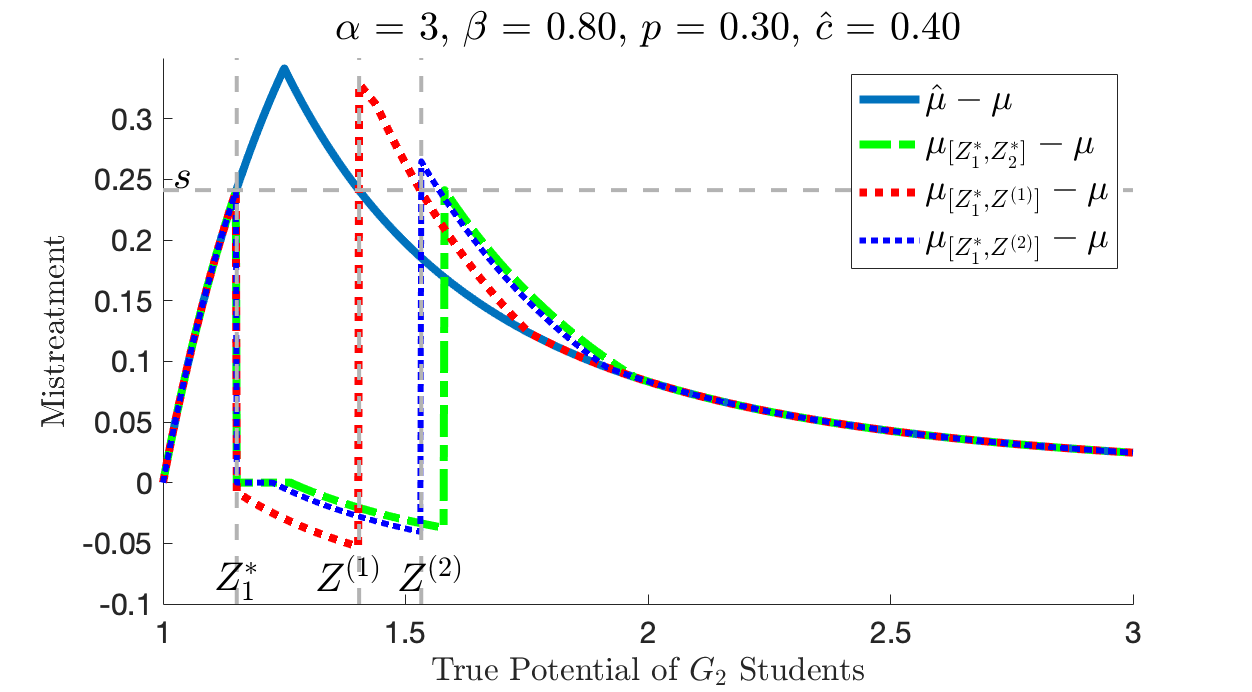
Figure 13: Plots of $\mu_{T}-\mu$ for sets $T$ constructed in Section 9.2.6.

9.3 Minimizing the aggregate amount of mistreatment received by all $G_{2}$ students

In this case, we restrict our attention to debiasing $G_{2}$ students whose potentials are in a connected set - which is a justifiable implementation in practice (otherwise a student might feel unfairly treated given that someone with a better potential as well as someone with a worse potential receives the voucher). This assumption also makes our analysis more tractable. In particular, let $\mathcal{T}^{c}(\widehat{c})\subseteq\mathcal{T}(\widehat{c})$ be all connected sets $T\in\mathcal{T}(\widehat{c})$. That is, $\mathcal{T}^{c}(\widehat{c}):=\{[t_{1},t_{2}]:\bar{F}_{1}(t_{1})-\bar{F}_{1}(t_{2})\leq\widehat{c}\}$. In addition, let $\mathcal{T}^{c}_{auc}(\widehat{c})$ be the collection of sets $T\in\mathcal{T}^{c}(\widehat{c})$ such that $\sigma(\mu_{T}-\mu)$ is minimized. The next result gives an explicit description of the set $\mathcal{T}^{c}_{auc}(\widehat{c})$ when assuming, again, (3) and additionally $p<0.5$.

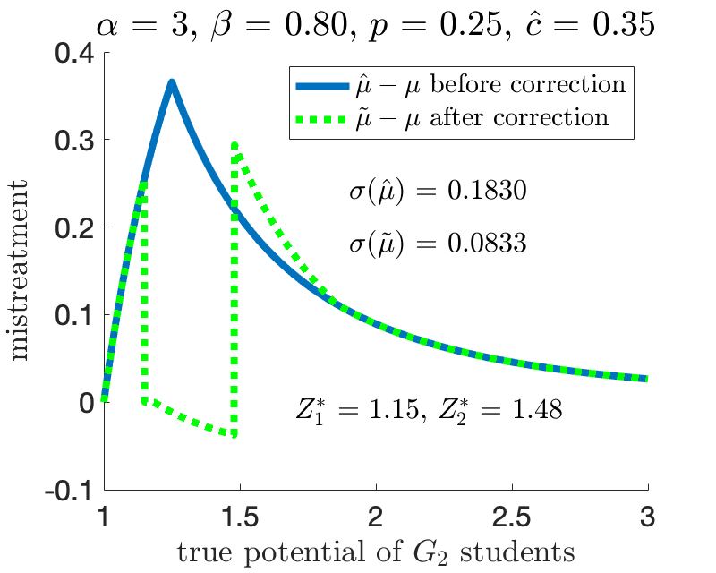
(a) optimal correction when $\widehat{c}$ is large

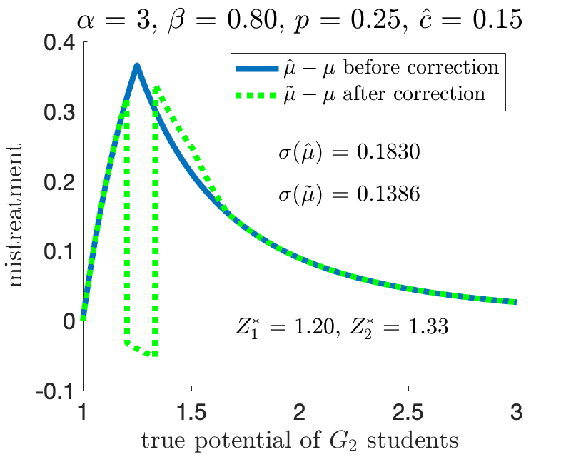
(b) optimal correction when $\widehat{c}$ is small

Figure 14: PAUC before and after optimal voucher correction.

Theorem 9.2

Assume $p<1-\beta^{\alpha}$ and $p<0.5$ Then $\mathcal{T}^{c}_{auc}(\widehat{c})$ is made of a unique set $T=[Z_{1}^{*},Z_{2}^{*}]$. If $\widehat{c}\geq\frac{(1-p)(1-\beta^{\alpha})}{2-p-\beta^{\alpha}-p\beta^{\alpha}+p\beta^{2\alpha}}$, then:

$$Z_{2}^{*}=\bigg{(}\frac{(1-p)(1-\widehat{c})}{p\beta^{\alpha}+\frac{1}{\beta^{\alpha}}-2p}\bigg{)}^{-\frac{1}{\alpha}}\quad\text{ and }\quad Z_{1}^{*}=\bigg{(}\frac{(1-p)(1-\widehat{c})}{p\beta^{\alpha}+\frac{1}{\beta^{\alpha}}-2p}+\widehat{c}\bigg{)}^{-\frac{1}{\alpha}},$$

and $\sigma(\mu_{[Z_{1}^{*},Z_{2}^{*}]})=\frac{1}{2}(1-p)(1-\beta^{\alpha})\left(\frac{(\frac{1}{\beta^{\alpha}}-p)(1-\widehat{c})^{2}}{p\beta^{\alpha}+\frac{1}{\beta^{\alpha}}-2p}\right)$, dropped from $\sigma(\widehat{\mu})=\frac{1}{2}(1-p)(1-\beta^{\alpha})$. Conversely, if $\widehat{c}\leq\frac{(1-p)(1-\beta^{\alpha})}{2-p-\beta^{\alpha}-p\beta^{\alpha}+p\beta^{2\alpha}}$, then:

$$Z_{2}^{*}=\bigg{(}\frac{(p\beta^{\alpha}-1)\widehat{c}+(1-p)}{(1-p)\frac{1}{\beta^{\alpha}}}\bigg{)}^{-\frac{1}{\alpha}}\quad\text{ and }\quad Z_{1}^{*}=\bigg{(}\frac{(p\beta^{\alpha}-1)\widehat{c}+(1-p)}{(1-p)\frac{1}{\beta^{\alpha}}}+\widehat{c}\bigg{)}^{-\frac{1}{\alpha}},$$

and $\sigma(\mu_{[Z_{1}^{*},Z_{2}^{*}]})=\frac{1}{2}(1-p)(1-\widehat{c})^{2}-\frac{1}{2}\beta^{\alpha}\left(\frac{[(p\beta^{\alpha}-1)\widehat{c}+(1-p)]^{2}}{1-p}+p\widehat{c}^{2}\right)$.

A pictorial representation of Theorem 9.2 is given in Figure 14. Again, two sub-figures are presented for two different choices of $\widehat{c}$. Figure 4(b) shows how much $\sigma(\mu_{[Z_{1}^{*},Z_{2}^{*}]})$ decreases as $\widehat{c}$, the amount of resources, increases.

9.4 Proof of Theorem 9.2

Assume $T=[Z_{1},Z_{2}]$ is the range of true potentials of $G_{2}$ students we want to debias. For simplicity, as in previous sections, let $\widetilde{\mu}$ denote $\mu_{T}$. In order to obtain the minimizer of $\sigma(\widetilde{\mu}-\mu)$, first, we want to compute $\sigma(\widetilde{\mu}-\mu)$ for each of the cases in Section 9.2. To start with, under the status quo, we have

$$\sigma(\widehat{\mu}-\mu) =(1-p)\left(\frac{1}{\beta^{\alpha}}-1\right)\int_{\frac{1}{\beta}}^{\infty}\left(\frac{1}{t}\right)^{\alpha}\frac{\alpha}{t^{\alpha+1}}dt+(1-p)\int_{1}^{\frac{1}{\beta}}\left(1-\left(\frac{1}{t}\right)^{\alpha}\right)\frac{\alpha}{t^{\alpha+1}}dt$$

$$=(1-p)\left(\frac{1}{\beta^{\alpha}}-1\right)\frac{1}{2}(\beta^{2\alpha}-0)+(1-p)\left(1-\beta^{\alpha}-\frac{1}{2}(1-\beta^{2\alpha})\right)$$

$$=\frac{1}{2}(1-p)(1-\beta^{\alpha}).$$

For $1\leq t_{1}\leq t_{2}\in\mathbb{R}\cup\{+\infty\}$, let

$$\sigma_{t_{1}}^{t_{2}}(f):=\int_{t_{1}}^{t_{2}}\max(f(t),0)dF_{1}(t)$$

for any function $f:[1,\infty]\rightarrow[0,1]$. When $t_{1}=1$ and $t_{2}=\infty$, we simply write $\sigma(f)$, which is consistent with previous notations. Note that with $\sigma(\widehat{\mu}-\mu)$ as a reference, it actually suffices to compute only $\sigma_{Z_{1}}^{Z_{2}/\beta}(\widetilde{\mu}-\mu)$, because minimizing $\sigma(\widetilde{\mu}-\mu)$ is equivalent to maximizing $\sigma_{Z_{1}}^{Z_{2}/\beta}(\widehat{\mu}-\mu)-\sigma_{Z_{1}}^{Z_{2}/\beta}(\widetilde{\mu}-\mu)$ given that $(\widehat{\mu}-\mu)(\theta)=(\widetilde{\mu}-\mu)(\theta)$ for all $\theta\in G_{2}$ such that $Z(\theta)\notin[Z_{1},Z_{2}/\beta]$.

In addition to giving an explicit formula for $\sigma_{Z_{1}}^{Z_{2}/\beta}(\widehat{\mu}-\mu)-\sigma_{Z_{1}}^{Z_{2}/\beta}(\widetilde{\mu}-\mu)$ in each case, we also analyze how this value changes (increase or decrease) with respect to $Z_{1}$ and $Z_{2}$.

9.4.1 CASE I: $\beta Z_{2}\geq Z_{1}$

Subcase 1. $1\leq\beta Z_{1}$. To compute the PAUC, we need to express $\widetilde{\mu}-\mu$ for all $\theta$ with $Z(\theta)\in[1,\infty)$ and $(\widetilde{\mu}-\mu)(\theta)>0$. In fact, all such pieces have been computed in the previous section. All pieces together, we have

$$(\widetilde{\mu}-\mu)(\theta)=\begin{cases}\displaystyle(\widehat{\mu}-\mu)(\theta)=(1-p)\left(1-\left(\frac{1}{Z(\theta)}\right)^{\alpha}\right)>0&\text{ if }1\leq Z(\theta)\leq\frac{1}{\beta},\\[5.69054pt] \displaystyle(\widehat{\mu}-\mu)(\theta)=(1-p)\left(\frac{1}{Z(\theta)}\right)^{\alpha}\left(\frac{1}{\beta^{\alpha}}-1\right)>0&\text{ if }\frac{1}{\beta}\leq Z(\theta)\leq Z_{1},\\[5.69054pt] \displaystyle 0&\text{ if }Z_{1}\leq Z(\theta)\leq\beta Z_{2},\\[5.69054pt] \displaystyle<0&\text{ if }\beta Z_{2}\leq Z(\theta)\leq Z_{2},\\[5.69054pt] \displaystyle\left(\frac{1}{Z(\theta)}\right)^{\alpha}\left(p+\frac{1}{\beta^{\alpha}}-1\right)-p\left(\frac{1}{Z_{2}}\right)^{\alpha}>0&\text{ if }Z_{2}\leq Z(\theta)\leq Z_{2}/\beta,\\[5.69054pt] \displaystyle(\widehat{\mu}-\mu)(\theta)=(1-p)\left(\frac{1}{Z(\theta)}\right)^{\alpha}\left(\frac{1}{\beta^{\alpha}}-1\right)>0&\text{ if }Z(\theta)\geq\beta Z_{2}.\end{cases}$$

The only necessary piece to integrate here is

$$\sigma_{Z_{2}}^{Z_{2}/\beta}(\widetilde{\mu}-\mu) =\left(p+\frac{1}{\beta^{\alpha}}-1\right)\int_{Z_{2}}^{Z_{2}/\beta}\left(\frac{1}{t}\right)^{\alpha}\frac{\alpha}{t^{\alpha+1}}dt-p\left(\frac{1}{Z_{2}}\right)^{\alpha}\int_{Z_{2}}^{Z_{2}/\beta}\frac{\alpha}{t^{\alpha+1}}dt$$

$$=\left(p+\frac{1}{\beta^{\alpha}}-1\right)\frac{1-\beta^{2\alpha}}{2}\left(\frac{1}{Z_{2}}\right)^{2\alpha}-p\left(\frac{1}{Z_{2}}\right)^{2\alpha}(1-\beta^{\alpha}).$$

Moreover, in this case, we have

$$\sigma_{Z_{1}}^{Z_{2}/\beta}(\widehat{\mu}-\mu) =(1-p)\left(\frac{1}{\beta^{\alpha}}-1\right)\int_{Z_{1}}^{Z_{2}/\beta}\left(\frac{1}{t}\right)^{\alpha}\frac{\alpha}{t^{\alpha+1}}dt$$

$$=(1-p)\left(\frac{1}{\beta^{\alpha}}-1\right)\frac{1}{2}\left(\left(\frac{1}{Z_{1}}\right)^{2\alpha}-\left(\frac{\beta}{Z_{2}}\right)^{2\alpha}\right).$$

Thus,

$$\sigma_{Z_{1}}^{Z_{2}/\beta}(\widehat{\mu}-\mu)-\sigma_{Z_{1}}^{Z_{2}/\beta}(\widetilde{\mu}-\mu) =\frac{(1-p)\left(\frac{1}{\beta^{\alpha}}-1\right)}{2}\left(\frac{1}{Z_{1}}\right)^{2\alpha}+\frac{p-p\beta^{\alpha}-\frac{1}{\beta^{\alpha}}+1}{2}\left(\frac{1}{Z_{2}}\right)^{2\alpha}.$$

Now, to analyze how this quantity changes with $Z_{1}$ and $Z_{2}$, we first simplify some of the terms, which will also be used in later sections. Let $x=(\frac{1}{Z_{2}})^{\alpha}\in[0,1]$ and let $(\frac{1}{Z_{1}})^{\alpha}=c+x\in[0,1]$ for some $c\leq\widehat{c}$. Also, let $g(x,c):=\sigma_{Z_{1}}^{Z_{2}/\beta}(\widehat{\mu}-\mu)-\sigma_{Z_{1}}^{Z_{2}/\beta}(\widetilde{\mu}-\mu)$. Then,

$$g(x,c)=\frac{(1-p)\left(\frac{1}{\beta^{\alpha}}-1\right)}{2}(c+x)^{2}+\frac{p-p\beta^{\alpha}-\frac{1}{\beta^{\alpha}}+1}{2}x^{2}.$$

We want to show that $g(x,c)$ increases as $x$ increases (or equivalently, as $Z_{2}$ decreases) and as $c$ increases (meaning that the constraint $(\frac{1}{Z_{1}})^{\alpha}-(\frac{1}{Z_{2}})^{\alpha}\leq\widehat{c}$ is effectively $(\frac{1}{Z_{1}})^{\alpha}-(\frac{1}{Z_{2}})^{\alpha}=\widehat{c}$). First,

$$\frac{\partial g(x,c)}{\partial c}=\underbrace{(1-p)\left(\frac{1}{\beta^{\alpha}}-1\right)}_{\geq 0}(c+x)\geq 0.$$

Next, rearranging the terms, we have

$$g(x,c)=\frac{p}{2}(2-\frac{1}{\beta^{\alpha}}-\beta^{\alpha})x^{2}+(1-p)\left(\frac{1}{\beta^{\alpha}}-1\right)cx+\text{const}.$$

Let

$$h(c):=-\frac{(1-p)\left(\frac{1}{\beta^{\alpha}}-1\right)c}{p(2-\frac{1}{\beta^{\alpha}}-\beta^{\alpha})}$$

be the peak of the parabola $g(x,c)$. For each given $c$, we want to show that $h(c)$ is always greater that the maximum possible $x$ in this case. If so, we have that $g(x,c)$ is an increasing function of $x$. Since $\beta Z_{2}\geq Z_{1}$, we have $c=(\frac{1}{Z_{1}})^{\alpha}-(\frac{1}{Z_{2}})^{\alpha}\geq(\frac{1}{Z_{2}})^{\alpha}(\frac{1}{\beta^{\alpha}}-1)=x(\frac{1}{\beta^{\alpha}}-1)$. Thus, it is enough to show

$$\frac{(1-p)\left(\frac{1}{\beta^{\alpha}}-1\right)^{2}}{p(\frac{1}{\beta^{\alpha}}+\beta^{\alpha}-2)}\geq 1\quad \Leftrightarrow\quad(1-p)\left(\frac{1}{\beta^{\alpha}}-1\right)^{2}\geq p(1-\beta^{\alpha})\left(\frac{1}{\beta^{\alpha}}-1\right)$$

$$\Leftrightarrow\quad(1-p)\left(\frac{1}{\beta^{\alpha}}-1\right)\geq p(1-\beta^{\alpha}).$$

The last inequality is true because of the assumption that $p<.5$ and $\frac{1}{\beta^{\alpha}}+\beta^{\alpha}-2\geq 0$.

Subcase 2. $\beta Z_{1}\leq 1\leq\beta Z_{2}$. The formula for $\widetilde{\mu}-\mu$ is similar to the previous case:

$$(\widetilde{\mu}-\mu)(\theta)=\begin{cases}\displaystyle(\widehat{\mu}-\mu)(\theta)=(1-p)\left(1-\left(\frac{1}{Z(\theta)}\right)^{\alpha}\right)>0&\text{ if }1\leq Z(\theta)\leq Z_{1},\\[5.69054pt] \displaystyle 0&\text{ if }Z_{1}\leq Z(\theta)\leq\beta Z_{2},\\[5.69054pt] \displaystyle<0&\text{ if }\beta Z_{2}\leq Z(\theta)\leq Z_{2},\\[5.69054pt] \displaystyle\left(\frac{1}{Z(\theta)}\right)^{\alpha}\left(p+\frac{1}{\beta^{\alpha}}-1\right)-p\left(\frac{1}{Z_{2}}\right)^{\alpha}>0&\text{ if }Z_{2}\leq Z(\theta)\leq Z_{2}/\beta,\\[5.69054pt] \displaystyle(\widehat{\mu}-\mu)(\theta)=(1-p)\left(\frac{1}{Z(\theta)}\right)^{\alpha}\left(\frac{1}{\beta^{\alpha}}-1\right)>0&\text{ if }Z(\theta)\geq\beta Z_{2}.\end{cases}$$

However, here, for the status quo baseline, we have

$$\sigma_{Z_{1}}^{Z_{2}/\beta}(\widehat{\mu}-\mu) =(1-p)\left(\frac{1}{\beta^{\alpha}}-1\right)\int_{1/\beta}^{Z_{2}/\beta}\left(\frac{1}{t}\right)^{\alpha}\frac{\alpha}{t^{\alpha+1}}dt+(1-p)\int_{Z_{1}}^{1/\beta}\left(1-\left(\frac{1}{t}\right)^{\alpha}\right)\frac{\alpha}{t^{\alpha+1}}dt$$

$$=\frac{(1-p)(\beta^{\alpha}-\beta^{2\alpha})}{2}\left(1-\left(\frac{1}{Z_{2}}\right)^{2\alpha}\right)+(1-p)\left[\left(\frac{1}{Z_{1}}\right)^{\alpha}-\beta^{\alpha}-\frac{1}{2}\left(\left(\frac{1}{Z_{1}}\right)^{2\alpha}-\beta^{2\alpha}\right)\right]$$

and thus,

$$\sigma_{Z_{1}}^{Z_{2}/\beta}(\widehat{\mu}-\mu)-\sigma_{Z_{1}}^{Z_{2}/\beta}(\widetilde{\mu}-\mu) =-\frac{1}{2}(1-p)\beta^{\alpha}+(1-p)\left(\left(\frac{1}{Z_{1}}\right)^{\alpha}-\frac{1}{2}\left(\frac{1}{Z_{1}}\right)^{2\alpha}\right)$$

$$+\frac{p-p\beta^{\alpha}-\frac{1}{\beta^{\alpha}}+1}{2}\left(\frac{1}{Z_{2}}\right)^{2\alpha}.$$

Now, for the analysis, similarly, write

$$g(x,c)=\text{const}+(1-p)\left((c+x)-\frac{1}{2}(c+x)^{2}\right)+\frac{p-p\beta^{\alpha}-\frac{1}{\beta^{\alpha}}+1}{2}x^{2}.$$

Then,

$$\frac{\partial g(x,c)}{\partial c}=(1-p)(1-(c+x))\geq 0$$

and rearranging the terms, we have

$$g(x,c)=\frac{2p-p\beta^{\alpha}-\frac{1}{\beta^{\alpha}}}{2}x^{2}+(1-p)(1-c)x+\text{const}.$$

We will show that $2p-p\beta^{\alpha}-\frac{1}{\beta^{\alpha}}\leq 0$ by showing $\beta^{\alpha}p(2-\beta^{\alpha})\leq 1$. This is true under assumption (3), which is $p\leq 1-\beta^{\alpha}$, because

$$\beta^{\alpha}p(2-\beta^{\alpha})\leq\beta^{\alpha}(1-\beta^{\alpha})(2-\beta^{\alpha})\leq 1,$$

where the last inequality is due to the fact that $\beta^{\alpha}\leq 1$. Hence, let

$$h_{\text{I}}(c)=\frac{(1-p)(1-c)}{p\beta^{\alpha}+\frac{1}{\beta^{\alpha}}-2p},$$

then $g(x,c)$ is an increasing function w.r.t. $x$ on $[0,h_{\text{I}}(c)]$ and is a decreasing function on $[h_{\text{I}}(c),1]$.

9.4.2 CASE II: $\beta Z_{2}\leq Z_{1}$

Subcase 1. $1\leq\beta Z_{1}$. Again, we want to express $\widetilde{\mu}-\mu$ for all $\theta$ such that $Z(\theta)\in[1,\infty)$ and $(\widetilde{\mu}-\mu)(\theta)>0$. All pieces together, we have

$$(\widetilde{\mu}-\mu)(\theta)=\begin{cases}\displaystyle(\widehat{\mu}-\mu)(\theta)=(1-p)\left(1-\left(\frac{1}{Z(\theta)}\right)^{\alpha}\right)&\text{ if }1\leq Z(\theta)\leq\frac{1}{\beta},\\[5.69054pt] \displaystyle(\widehat{\mu}-\mu)(\theta)=(1-p)\left(\frac{1}{Z(\theta)}\right)^{\alpha}\left(\frac{1}{\beta^{\alpha}}-1\right)&\text{ if }\frac{1}{\beta}\leq Z(\theta)\leq Z_{1},\\[5.69054pt] \displaystyle<0&\text{ if }Z_{1}\leq Z(\theta)\leq Z_{2},\\[5.69054pt] \displaystyle\left(\frac{1}{Z(\theta)}\right)^{\alpha}(1-p)\left(\frac{1}{\beta^{\alpha}}-1\right)+p\left(\left(\frac{1}{Z_{1}}\right)^{\alpha}-\left(\frac{1}{Z_{2}}\right)^{\alpha}\right)&\text{ if }Z_{2}\leq Z(\theta)\leq Z_{1}/\beta,\\[5.69054pt] \displaystyle\left(\frac{1}{Z(\theta)}\right)^{\alpha}\left(p+\frac{1}{\beta^{\alpha}}-1\right)-p\left(\frac{1}{Z_{2}}\right)^{\alpha}&\text{ if }Z_{1}/\beta\leq Z(\theta)\leq Z_{2}/\beta,\\[5.69054pt] \displaystyle(\widehat{\mu}-\mu)(\theta)=(1-p)\left(\frac{1}{Z(\theta)}\right)^{\alpha}\left(\frac{1}{\beta^{\alpha}}-1\right)>0&\text{ if }Z(\theta)\geq\beta Z_{2}.\end{cases}$$

As subcase 1. of Section 9.4.1, for $\widehat{\mu}-\mu$, we have

$$\sigma_{Z_{1}}^{Z_{2}/\beta}(\widehat{\mu}-\mu)=(1-p)\left(\frac{1}{\beta^{\alpha}}-1\right)\frac{1}{2}\left(\left(\frac{1}{Z_{1}}\right)^{2\alpha}-\left(\frac{\beta}{Z_{2}}\right)^{2\alpha}\right),$$

and for $\widetilde{\mu}-\mu$, we need to compute the integral of the following two pieces.

$$\sigma_{Z_{2}}^{Z_{1}/\beta}(\widetilde{\mu}-\mu) =(1-p)\left(\frac{1}{\beta^{\alpha}}-1\right)\int_{Z_{2}}^{Z_{1}/\beta}\left(\frac{1}{t}\right)^{\alpha}\frac{\alpha}{t^{\alpha+1}}dt+p\left(\left(\frac{1}{Z_{1}}\right)^{\alpha}-\left(\frac{1}{Z_{2}}\right)^{\alpha}\right)\int_{Z_{2}}^{Z_{1}/\beta}\frac{\alpha}{t^{\alpha+1}}dt$$

$$=\frac{(1-p)\left(\frac{1}{\beta^{\alpha}}-1\right)}{2}\left(\left(\frac{1}{Z_{2}}\right)^{2\alpha}-(\frac{\beta}{Z_{1}})^{2\alpha}\right)+p\left(\left(\frac{1}{Z_{1}}\right)^{\alpha}-\left(\frac{1}{Z_{2}}\right)^{\alpha}\right)\left(\left(\frac{1}{Z_{2}}\right)^{\alpha}-\left(\frac{\beta}{Z_{1}}\right)^{\alpha}\right);$$

$$\sigma_{Z_{1}/\beta}^{Z_{2}/\beta}(\widetilde{\mu}-\mu) =\left(p+\frac{1}{\beta^{\alpha}}-1\right)\int_{Z_{1}/\beta}^{Z_{2}/\beta}\left(\frac{1}{t}\right)^{\alpha}\frac{\alpha}{t^{\alpha+1}}dt-p\left(\frac{1}{Z_{2}}\right)^{\alpha}\int_{Z_{1}/\beta}^{Z_{2}/\beta}\frac{\alpha}{t^{\alpha+1}}dt$$

$$=\frac{\left(p+\frac{1}{\beta^{\alpha}}-1\right)\beta^{2\alpha}}{2}\left(\left(\frac{1}{Z_{1}}\right)^{2\alpha}-\left(\frac{1}{Z_{2}}\right)^{2\alpha}\right)-p\beta^{\alpha}\left(\frac{1}{Z_{2}}\right)^{\alpha}\left(\left(\frac{1}{Z_{1}}\right)^{\alpha}-\left(\frac{1}{Z_{2}}\right)^{\alpha}\right).$$

Hence,

$$\sigma_{Z_{1}}^{Z_{2}/\beta}(\widehat{\mu}-\mu)-\sigma_{Z_{1}}^{Z_{2}/\beta}(\widetilde{\mu}-\mu) =\left(\frac{1}{Z_{1}}\right)^{2\alpha}\left(\frac{(1-p)\left(\frac{1}{\beta^{\alpha}}-1\right)+p\beta^{\alpha}}{2}\right)$$

$$-\left(\frac{1}{Z_{2}}\right)^{2\alpha}\left(\frac{(1-p)\left(\frac{1}{\beta^{\alpha}}-1\right)+p\beta^{\alpha}}{2}\right)$$

$$+p\left(\frac{1}{Z_{2}}\right)^{2\alpha}-p\left(\frac{1}{Z_{1}}\right)^{\alpha}\left(\frac{1}{Z_{2}}\right)^{\alpha}.$$

Now, for the analysis, let $A=[(1-p)(\frac{1}{\beta^{\alpha}}-1)+p\beta^{\alpha}]/2\geq 0$. Then,

$$g(x,c)=A(c+x)^{2}-Ax^{2}+px^{2}-p(c+x)(x).$$

First, we have

$$\frac{\partial g(x,c)}{\partial c}=2A(c+x)-px=2Ac+(2A-p)x.$$

Under the assumption that $1-p>\beta^{\alpha}$, we have $2A-p\geq\beta^{\alpha}(\frac{1}{\beta^{\alpha}}-1)+p\beta^{\alpha}+\beta^{\alpha}-1=p\beta^{\alpha}\geq 0$. Therefore, $\frac{\partial g(x,c)}{\partial c}\geq 0$. Next, rearranging the terms, we have

$$g(x,c)=c(2A-p)x+\text{const},$$

and thus, $g(x,c)$ is an increasing function on $x$.

Subcase 2. $\beta Z_{1}\leq 1\leq\beta Z_{2}$. Similar to the previous case, the formula for $\widetilde{\mu}-\mu$ is as follows:

$$(\widetilde{\mu}-\mu)(\theta)=\begin{cases}\displaystyle(\widehat{\mu}-\mu)(\theta)=(1-p)\left(1-\left(\frac{1}{Z(\theta)}\right)^{\alpha}\right)&\text{ if }1\leq Z(\theta)\leq Z_{1},\\[5.69054pt] \displaystyle<0&\text{ if }Z_{1}\leq Z(\theta)\leq Z_{2},\\[5.69054pt] \displaystyle\left(\frac{1}{Z(\theta)}\right)^{\alpha}(1-p)\left(\frac{1}{\beta^{\alpha}}-1\right)+p\left(\left(\frac{1}{Z_{1}}\right)^{\alpha}-\left(\frac{1}{Z_{2}}\right)^{\alpha}\right)&\text{ if }Z_{2}\leq Z(\theta)\leq Z_{1}/\beta,\\[5.69054pt] \displaystyle\left(\frac{1}{Z(\theta)}\right)^{\alpha}\left(p+\frac{1}{\beta^{\alpha}}-1\right)-p\left(\frac{1}{Z_{2}}\right)^{\alpha}&\text{ if }Z_{1}/\beta\leq Z(\theta)\leq Z_{2}/\beta,\\[5.69054pt] \displaystyle(\widehat{\mu}-\mu)(\theta)=(1-p)\left(\frac{1}{Z(\theta)}\right)^{\alpha}\left(\frac{1}{\beta^{\alpha}}-1\right)>0&\text{ if }Z(\theta)\geq\beta Z_{2}.\end{cases}$$

Same as subcase 2. of Section 9.4.1, we have

$$\sigma_{Z_{1}}^{Z_{2}/\beta}(\widehat{\mu}-\mu) =\frac{(1-p)(\beta^{\alpha}-\beta^{2\alpha})}{2}\left(1-\left(\frac{1}{Z_{2}}\right)^{2\alpha}\right)+(1-p)\left[\left(\frac{1}{Z_{1}}\right)^{\alpha}-\beta^{\alpha}-\frac{1}{2}\left(\left(\frac{1}{Z_{1}}\right)^{2\alpha}-\beta^{2\alpha}\right)\right].$$

Note the components of interest for $\widetilde{\mu}-\mu$ have the same expression as in the previous section. Thus, using the expression for the integrals from before, we have

$$\sigma_{Z_{1}}^{Z_{2}/\beta}(\widehat{\mu}-\mu)-\sigma_{Z_{1}}^{Z_{2}/\beta}(\widetilde{\mu}-\mu) =-\frac{1}{2}(1-p)\beta^{\alpha}+\left(\frac{1}{Z_{1}}\right)^{2\alpha}\bigg{(}\frac{-(1-p)+p\beta^{\alpha}}{2}\bigg{)}+(1-p)\left(\frac{1}{Z_{1}}\right)^{\alpha}$$

$$-\left(\frac{1}{Z_{2}}\right)^{2\alpha}\bigg{(}\frac{(1-p)\left(\frac{1}{\beta^{\alpha}}-1\right)+p\beta^{\alpha}}{2}\bigg{)}+p\left(\frac{1}{Z_{2}}\right)^{2\alpha}-p\left(\frac{1}{Z_{1}}\right)^{\alpha}\left(\frac{1}{Z_{2}}\right)^{\alpha}.$$

For the analysis, again let $A=[(1-p)(\frac{1}{\beta^{\alpha}}-1)+p\beta^{\alpha}]/2\geq 0$ and $B=[-(1-p)+p\beta^{\alpha}]/2$. Since $p<.5$, we have $B\leq 0$. Then, we can write

$$g(x,c)=\text{const}+B(c+x)^{2}+(1-p)(c+x)-Ax^{2}+px^{2}-p(c+x)(x).$$

First, we have

$$\frac{\partial g(x,c)}{\partial c}=2B(c+x)+(1-p)-px=(-(1-p)+p\beta^{\alpha})(c+x)+[(1-p)-px].$$

Since $x=(\frac{1}{Z_{2}})^{\alpha}\leq\beta^{\alpha}$, we have $[(1-p)-px]\geq(1-p)-p\beta^{\alpha}$ and thus, together with the fact that $c+x\leq 1$, we have

$$\frac{\partial g(x,c)}{\partial c}\geq((1-p)-p\beta^{\alpha})(1-(c+x))\geq 0.$$

Next, after rearranging the terms, we have

$$g(x,c) =(B-A)x^{2}+\big{[}2Bc+(1-p)-pc\big{]}x+\text{const}$$

$$=\frac{-(1-p)\frac{1}{\beta^{\alpha}}}{2}x^{2}+\big{[}(p\beta^{\alpha}-1)c+(1-p)\big{]}x+\text{const}.$$

We will show that in this case, we must have $\big{[}(p\beta^{\alpha}-1)c+(1-p)\big{]}\geq 0$. First, note that since $\beta Z_{2}\leq Z_{1}$, and $Z_{2}\geq\frac{1}{\beta}$, we have

$$c=\left(\frac{1}{Z_{1}}\right)^{\alpha}-\left(\frac{1}{Z_{2}}\right)^{\alpha}\leq\left(\frac{1}{\beta^{\alpha}}-1\right)\left(\frac{1}{Z_{2}}\right)^{\alpha}\leq\left(\frac{1}{\beta^{\alpha}}-1\right)\beta^{\alpha}=1-\beta^{\alpha}.$$

Thus, to show $\big{[}(p\beta^{\alpha}-1)c+(1-p)\big{]}\geq 0$, it is enough to show that $\big{[}(p\beta^{\alpha}-1)(1-\beta^{\alpha})+(1-p)\big{]}\geq 0$, which is equivalent to $p(\beta^{\alpha}(1-\beta^{\alpha})-1)+\beta^{\alpha}\geq 0$. Under the assumption that $p<1-\beta^{\alpha}$ and with the fact that $\beta^{\alpha}(1-\beta^{\alpha})-1\leq 0$, we have

$$p(\beta^{\alpha}(1-\beta^{\alpha})-1)+\beta^{\alpha}\geq(1-\beta^{\alpha})(\beta^{\alpha}(1-\beta^{\alpha})-1)+\beta^{\alpha}=(\beta^{\alpha})^{3}-2(\beta^{\alpha})^{2}+3\beta^{\alpha}-1\geq 0,$$

where the last inequality is because $f(t):=t^{3}-2t^{2}+3t-1$ is nonnegative when $t\geq 0$. Now, let

$$h_{\text{II}}(c)=\frac{(p\beta^{\alpha}-1)c+(1-p)}{(1-p)\frac{1}{\beta^{\alpha}}},$$

then $g(x,c)$ is an increasing function on $[0,h_{\text{II}}(c)]$ and is a decreasing function on $[h_{\text{II}}(c),1]$.

Subcase 3. $\beta Z_{2}\leq 1$. Again, we want to express $\widetilde{\mu}-\mu$ for all $\theta$ such that $Z(\theta)\in[1,\infty)$ and $(\widetilde{\mu}-\mu)(\theta)\geq 0$. Combining all pieces, we have

$$(\widetilde{\mu}-\mu)(\theta)=\begin{cases}\displaystyle(\widehat{\mu}-\mu)(\theta)=(1-p)\left(1-\left(\frac{1}{Z(\theta)}\right)^{\alpha}\right)&\text{ if }1\leq Z(\theta)\leq Z_{1},\\[5.69054pt] \displaystyle\leq 0&\text{ if }Z_{1}\leq Z(\theta)\leq Z_{2},\\[5.69054pt] \displaystyle(1-p)\left(1-\left(\frac{1}{Z(\theta)}\right)^{\alpha}\right)+p\left(\left(\frac{1}{Z_{1}}\right)^{\alpha}-\left(\frac{1}{Z_{2}}\right)^{\alpha}\right)&\text{ if }Z_{2}\leq Z(\theta)\leq 1/\beta,\\[5.69054pt] \displaystyle\left(\frac{1}{Z(\theta)}\right)^{\alpha}(1-p)\left(\frac{1}{\beta^{\alpha}}-1\right)+p\left(\left(\frac{1}{Z_{1}}\right)^{\alpha}-\left(\frac{1}{Z_{2}}\right)^{\alpha}\right)&\text{ if }1/\beta\leq Z(\theta)\leq Z_{1}/\beta,\\[5.69054pt] \displaystyle\left(\frac{1}{Z(\theta)}\right)^{\alpha}\left(p+\frac{1}{\beta^{\alpha}}-1\right)-p\left(\frac{1}{Z_{2}}\right)^{\alpha}&\text{ if }Z_{1}/\beta\leq Z(\theta)\leq Z_{2}/\beta,\\[5.69054pt] \displaystyle(\widehat{\mu}-\mu)(\theta)=(1-p)\left(\frac{1}{Z(\theta)}\right)^{\alpha}\left(\frac{1}{\beta^{\alpha}}-1\right)>0&\text{ if }Z(\theta)\geq\beta Z_{2}.\end{cases}$$

For $\widehat{\mu}-\mu$, as in subcase 2, we have

$$\sigma_{Z_{1}}^{Z_{2}/\beta}(\widehat{\mu}-\mu) =\frac{(1-p)(\beta^{\alpha}-\beta^{2\alpha})}{2}\left(1-\left(\frac{1}{Z_{2}}\right)^{2\alpha}\right)+(1-p)\left[\left(\frac{1}{Z_{1}}\right)^{\alpha}-\beta^{\alpha}-\frac{1}{2}\left(\left(\frac{1}{Z_{1}}\right)^{2\alpha}-\beta^{2\alpha}\right)\right].$$

For $\widetilde{\mu}-\mu$, the component of $\theta\in[Z_{1}/\beta,Z_{2}/\beta]$ is the same as in subcase 1 of this section, which is

$$\sigma_{Z_{1}/\beta}^{Z_{2}/\beta}(\widetilde{\mu}-\mu) =\frac{\left(p+\frac{1}{\beta^{\alpha}}-1\right)\beta^{2\alpha}}{2}\left(\left(\frac{1}{Z_{1}}\right)^{2\alpha}-\left(\frac{1}{Z_{2}}\right)^{2\alpha}\right)-p\beta^{\alpha}\left(\frac{1}{Z_{2}}\right)^{\alpha}\left(\left(\frac{1}{Z_{1}}\right)^{\alpha}-\left(\frac{1}{Z_{2}}\right)^{\alpha}\right),$$

and we only have to integrate the other two components:

$$\sigma_{Z_{2}}^{1/\beta}(\widetilde{\mu}-\mu) =(1-p)\int_{Z_{2}}^{1/\beta}\left(1-\left(\frac{1}{t}\right)^{\alpha}\right)\frac{\alpha}{t^{\alpha+1}}dt+p\left(\left(\frac{1}{Z_{1}}\right)^{\alpha}-\left(\frac{1}{Z_{2}}\right)^{\alpha}\right)\int_{Z_{2}}^{1/\beta}\frac{\alpha}{t^{\alpha+1}}dt$$

$$=(1-p)\left[\left(\frac{1}{Z_{2}}\right)^{\alpha}-\beta^{\alpha}-\frac{1}{2}\big{(}\left(\frac{1}{Z_{2}}\right)^{2\alpha}-\beta^{2\alpha}\big{)}\right]+p\left(\left(\frac{1}{Z_{1}}\right)^{\alpha}-\left(\frac{1}{Z_{2}}\right)^{\alpha}\right)\left(\left(\frac{1}{Z_{2}}\right)^{\alpha}-\beta^{\alpha}\right);$$

$$\sigma_{1/\beta}^{Z_{1}/\beta}(\widetilde{\mu}-\mu) =(1-p)\left(\frac{1}{\beta^{\alpha}}-1\right)\int_{1/\beta}^{Z_{1}/\beta}\left(\frac{1}{t}\right)^{\alpha}\frac{\alpha}{t^{\alpha+1}}dt+p\left(\left(\frac{1}{Z_{1}}\right)^{\alpha}-\left(\frac{1}{Z_{2}}\right)^{\alpha}\right)\int_{1/\beta}^{Z_{1}/\beta}\frac{\alpha}{t^{\alpha+1}}dt$$

$$=\frac{(1-p)\left(\frac{1}{\beta^{\alpha}}-1\right)\beta^{2\alpha}}{2}\left[1-\left(\frac{1}{Z_{1}}\right)^{2\alpha}\right]+p\left(\left(\frac{1}{Z_{1}}\right)^{\alpha}-\left(\frac{1}{Z_{2}}\right)^{\alpha}\right)\left(\beta^{\alpha}-\left(\frac{\beta}{Z_{1}}\right)^{\alpha}\right).$$

Putting them together, we have

$$\sigma_{Z_{1}}^{Z_{2}/\beta}(\widehat{\mu}-\mu)-\sigma_{Z_{1}}^{Z_{2}/\beta}(\widetilde{\mu}-\mu) =\left(\frac{1}{Z_{1}}\right)^{2\alpha}\left(\frac{-(1-p)+p\beta^{\alpha}}{2}\right)+(1-p)\left(\frac{1}{Z_{1}}\right)^{\alpha}$$

$$-\left(\frac{1}{Z_{2}}\right)^{2\alpha}\left(\frac{-(1-p)+p\beta^{\alpha}}{2}\right)-(1-p)\left(\frac{1}{Z_{2}}\right)^{\alpha}$$

$$+p\left(\frac{1}{Z_{2}}\right)^{2\alpha}-p\left(\frac{1}{Z_{1}}\right)^{\alpha}\left(\frac{1}{Z_{2}}\right)^{\alpha}.$$

Lastly, for the analysis, write

$$g(x,c)=B(c+x)^{2}+(1-p)(c+x)-Bx^{2}-(1-p)x+px^{2}-p(c+x)x.$$

Rearranging the terms, we have

$$g(x,c)=\big{[}2Bc+(1-p)-(1-p)-pc\big{]}x=(-1+p\beta^{\alpha})cx.$$

Thus, $g(x,c)$ is a decreasing function in $x$. In addition, taking the partial derivative w.r.t. $c$, we have

$$\frac{\partial g(x,c)}{\partial c}=2B(c+x)+(1-p)-px=(-(1-p)+p\beta^{\alpha})(c+x)+[(1-p)-px].$$

The sign of $\frac{\partial g(x,c)}{\partial c}$ is actually not clear in this subcase. But for the purpose of finding the minimizer of $\sigma(\widetilde{\mu}-\mu)$, this is not important because for a fixed value of $c$, $g(x,c)$ achieves its maximum when $x$ is of the value such that $[Z_{1},Z_{2}]$ is of subcase 2, of either case I or case II.

9.4.3 Computing the optimal range for vouchers

In Figure 15, we demonstrate how the type of range $[Z_{1},Z_{2}]$ evolves as it moves to the right along the axis given that $(\frac{1}{Z_{1}})^{\alpha}-(\frac{1}{Z_{2}})^{\alpha}=\widehat{c}$ is fixed.

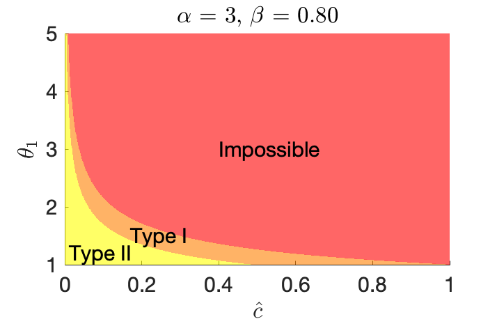
Figure 15: Change in type of $[Z_{1},Z_{2}]$ as $Z_{1}$ increases given $(\frac{1}{Z_{1}})^{\alpha}-(\frac{1}{Z_{2}})^{\alpha}=\widehat{c}$ and fixed parameters.

Although the evolution is different depending the value of $\widehat{c}$, for a fixed value of $\widehat{c}$, as $Z_{1}$ gets larger (or equivalently as $Z_{2}$ gets larger, or as $x:=(\frac{1}{Z_{2}})^{\alpha}$ gets smaller), the range $[Z_{1},Z_{2}]$ goes from type II to type I. In particular, for each value of $\widehat{c}$, such transition happens exactly when $\beta Z_{2}=Z_{1}$. That is, when

$$\widehat{c}=\left(\frac{1}{\beta^{\alpha}}-1\right)\left(\frac{1}{Z_{2}}\right)^{\alpha}\quad\Leftrightarrow\quad\left(\frac{1}{Z_{2}}\right)^{\alpha}=\frac{\widehat{c}\beta^{\alpha}}{1-\beta^{\alpha}}$$

Now, for each fixed value of $\widehat{c}$, Figure 16 plots $\sigma(\widehat{\mu}-\mu)-\sigma(\widetilde{\mu}-\mu)$ against $Z_{1}$. It also shows that as $Z_{1}$ increases, how the interval $[Z_{1},Z_{2}]$ changes by cases.

With simple algebra, one can easily check that when $\widehat{c}=\frac{(1-p)(1-\beta^{\alpha})}{2-p-\beta^{\alpha}-p\beta^{\alpha}+p\beta^{2\alpha}}$, we have that $h_{\text{I}}(\widehat{c})=h_{\text{II}}(\widehat{c})=\frac{\widehat{c}\beta^{\alpha}}{1-\beta^{\alpha}}$. Therefore,

• When $\widehat{c}\geq\frac{(1-p)(1-\beta^{\alpha})}{2-p-\beta^{\alpha}-p\beta^{\alpha}+p\beta^{2\alpha}}$, we have $h_{\text{I}}(\widehat{c})\leq\frac{\widehat{c}\beta^{\alpha}}{1-\beta^{\alpha}}$ and $h_{\text{II}(\widehat{c})}\leq\frac{\widehat{c}\beta^{\alpha}}{1-\beta^{\alpha}}$. Thus, the maximum of $\sigma(\widehat{\mu}-\mu)-\sigma(\widetilde{\mu}-\mu)$ is achieved when $x=h_{\text{I}}(\widehat{c})$.

• When $\widehat{c}\leq\frac{(1-p)(1-\beta^{\alpha})}{2-p-\beta^{\alpha}-p\beta^{\alpha}+p\beta^{2\alpha}}$, we have $h_{\text{I}}(\widehat{c})\geq\frac{\widehat{c}\beta^{\alpha}}{1-\beta^{\alpha}}$ and $h_{\text{II}(\widehat{c})}\geq\frac{\widehat{c}\beta^{\alpha}}{1-\beta^{\alpha}}$. Thus, the maximum of $\sigma(\widehat{\mu}-\mu)-\sigma(\widetilde{\mu}-\mu)$ is achieved when $x=h_{\text{II}}(\widehat{c})$.

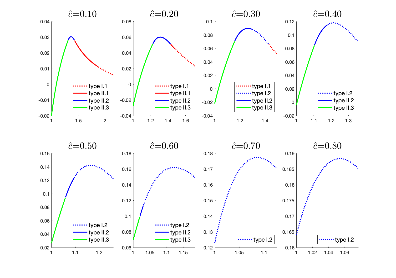
Figure 16: For fixed values of $\widehat{c}$, the function of $\sigma(\widehat{\mu}-\mu)-\sigma(\widetilde{\mu}-\mu)$ on $Z_{1}$

10 Details on the empirical evaluations when hypothesis are perturbed

In this section, we give more details on the empirical evaluation of our results with perturbed data discussed in Section 6.1. Results are also reported in Figure 17, Figure 18(a), Figure 18(b). (when only one assumption is relaxed) and Figure 19 (when all three assumptions are relaxed).

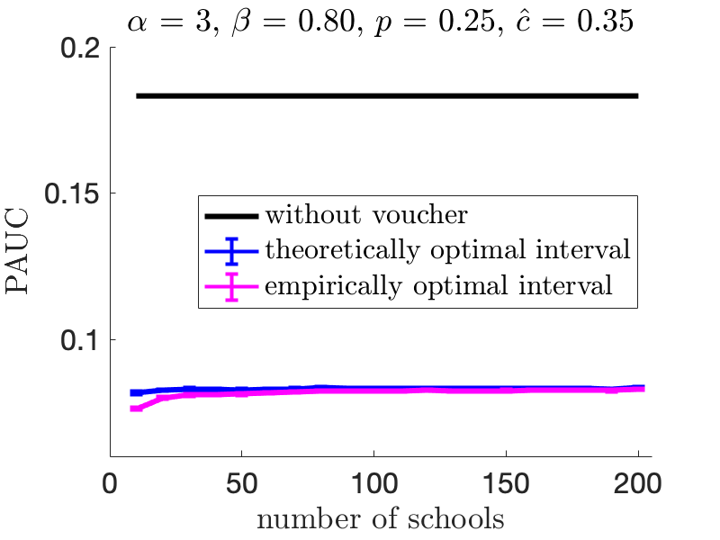
Figure 17: Assuming a constant number of $100$ students per school, we compare the PAUC when debiasing $G_{2}$ students in the theoretically optimal interval given in Theorem 9.2 versus the PAUC when debiasing $G_{2}$ students in the empirically optimal interval. The PAUC without intervention is presented as a baseline.

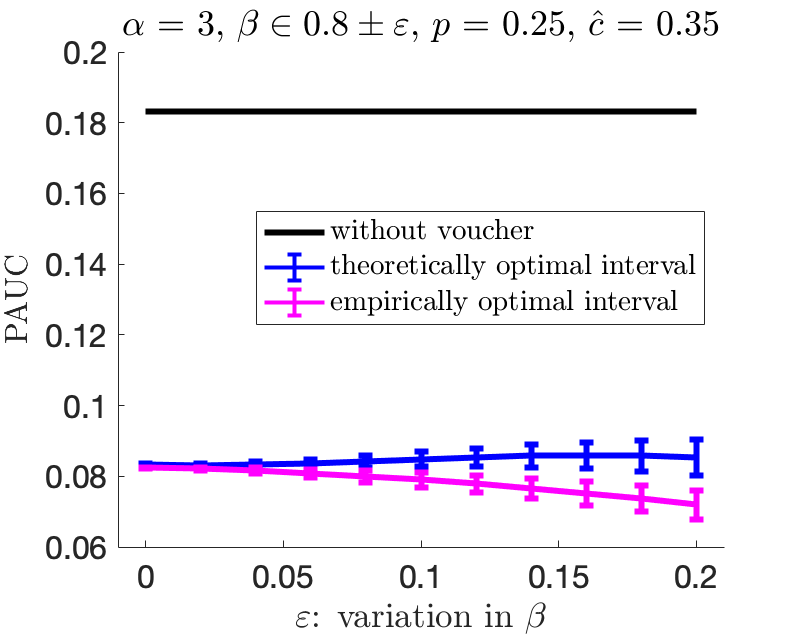
(a) Each $G_{2}$ student’s discount factor $\beta$ is drawn uniformly randomly from interval $[0.8-\varepsilon,0.8+\varepsilon]$.

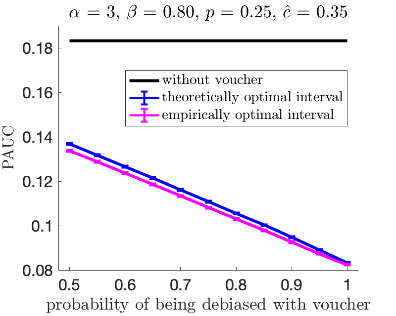
(b) Each $G_{2}$ student who is offered a voucher is able to reveal his true potential with certain probability.

Figure 18: All simulations are carried out on instances with $10,000$ students and $100$ schools, where each school has a capacity of $100$ students. We compare the PAUC when debiasing $G_{2}$ students in the theoretically optimal interval given in Theorem 9.2 versus the PAUC when debiasing $G_{2}$ students in the empirically optimal interval. The PAUC without intervention is presented as a baseline.

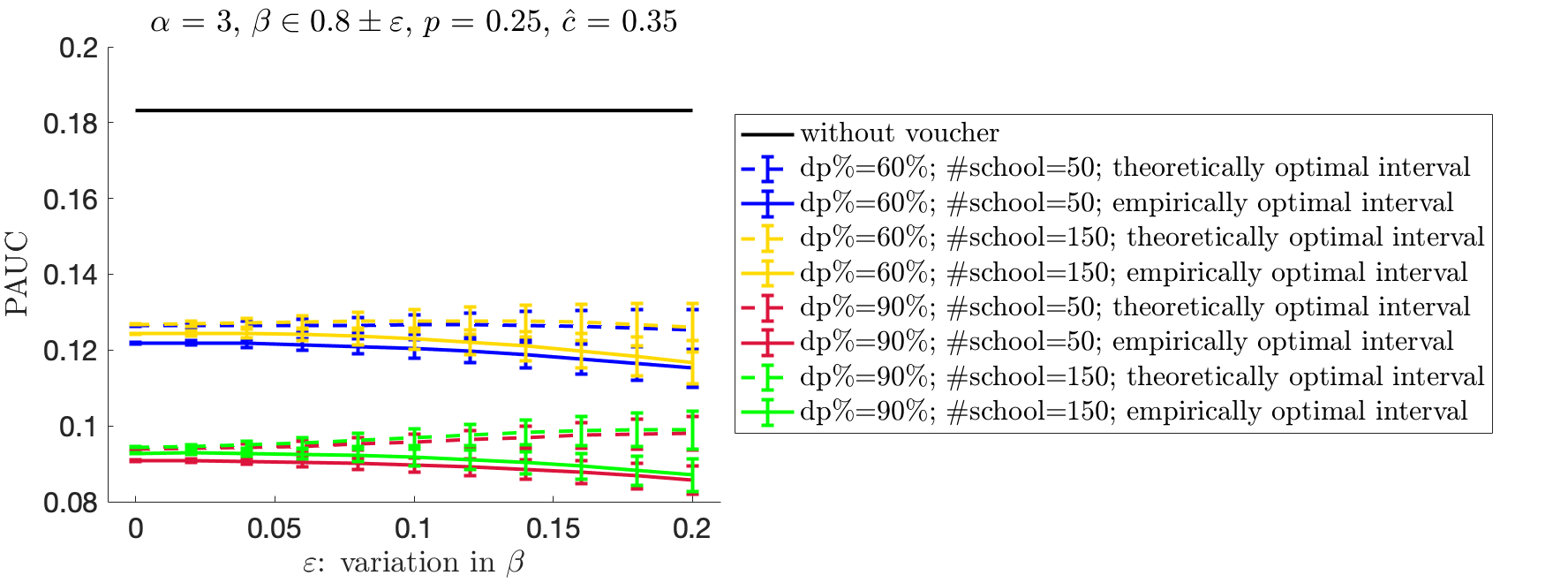
Figure 19: Assuming each school has $100$ seats, we carried out four sets of experiments, where in each experiment, the variation $\varepsilon$ in the discount factor $\beta$ varies from $0$ to $0.20$. These experiments differ in debiasing probability, either $60\%$ or $90\%$, and/or the number of schools, either $50$ or $150$. We compare the PAUC when debiasing $G_{2}$ students in the theoretically optimal interval given in Theorem 9.2 versus the PAUC when debiasing $G_{2}$ students in the empirically optimal interval. The PAUC without intervention is presented as a baseline.

From continuous to discrete. We first investigate how accurately the results on our model translate to a model where both sides of the market are discrete. Assuming a constant number of $100$ students per school, we carried out a set of experiments where the number of schools ranges from $10$ to $200$. Due to the randomness resulting from discretization, for each experiment, we conducted $100$ simulations and report here their mean and standard error of the mean in Figure 17. In fact, the standard errors are very small and thus they do not show in the figure. When the number of schools is more than 50, the theoretically optimal interval given in Theorem 9.2 for the continuous-continuous model performs well for the discrete model as well. And regardless of the magnitude of discretization (i.e., number of schools), the theoretical formula is able to reduce PAUC significantly from the PAUC under the situation without any intervention (by close to $50\%$).

Due to this result, for the following experiments, simulations are run on instances with $10,000$ students and $100$ schools, and each school has a capacity of $100$ students.

Non-constant bias. We next investigate the assumption of constant discount factor $\beta$ for all $G_{2}$ students. In this set of experiments, we allow $\beta$ to vary among $G_{2}$ students by different amounts. Results are shown in Figure 18(a). When variation in $\beta$ is small (i.e., $\varepsilon$ is small), the PAUC obtained using the formula in Theorem 9.2 is close the empirically optimal value. However, as the amount of variation in $\beta$ increases, the discrepancy between the theoretically optimal value the empirical one increases. However, debiasing $G_{2}$ students in the theoretically optimal interval can regardless reduce the PAUC significantly from the situation without any intervention.

Students may not use vouchers. We then investigate the assumption that once a $G_{2}$ student is offered the voucher, (s)he is able to reveal his true potential with $100\%$ probability. In this set of experiments, we vary this probability from $50\%$ to $100\%$. Results are presented in Figure 18(b). As the probability decreases, the optimal PAUC, theoretically as well as empirically, increases. This increase is intuitive because when debiasing probability is small, many vouchers are essentially “wasted”. However, the discrepancy between the PAUC under the theoretically optimal interval and that under the empirically optimal interval is relatively small, even when the debiasing probability is only $50\%$. Again, standard errors are very small and thus do not appear in the figure.

Simultaneous relaxation of all the three modeling assumptions. As a final step, we combine the three above-mentioned situations together. The results are summarized in Figure 19. For a fixed level of debiasing probability and a number of schools, the discrepancy between the theoretically optimal PAUC and the empirically optimal PAUC (i.e., comparing solid lines and dashed lines of the same color) is comparable to those seen in Figure 18(a). That is, the influence of variation $\varepsilon$ is uniform across different levels of debiasing probability and/or discretization. In addition, observe that the differences between the solid lines and dashed lines are similar for different levels of variation $\varepsilon$ cross four different colors (i.e., four different set of experiments with different combination of low or high debiasing probability and small or large number of schools). This implies that the differences between the theoretically optimal PAUC and the empirically optimal PAUC can be explained mostly by the variation $\varepsilon$ in the bias factor. In other words, varying debiasing probability and/or varying the number of schools do not, in general, result in a notably different discrepancy between the theoretically optimal solution and the empirically optimal solution.

Biased group is the majority. So far, we have been assuming $p$ to be small. That is, we assume the student group that is experiencing bias (i.e., $G_{2}$ students) is the minority. It is interesting also to consider the case where $G_{2}$ students form a majority group, and analyze how bias in the system affects students and schools differently. We summarize our findings in Figure 20 and Figure 21. Again, middle-performing $G_{2}$ students are the ones who are heavily penalized, although when $p>0.5$, the overall magnitude of mistreatment faced by $G_{2}$ students is smaller when compared to the benefits $G_{1}$ students receive, especially to the $G_{1}$ students with lower potentials. The perspective from schools’ point of view is similar to when $p$ is small. That is, schools are not significantly influenced by the bias in evaluation and thus do not have much incentives for a change.

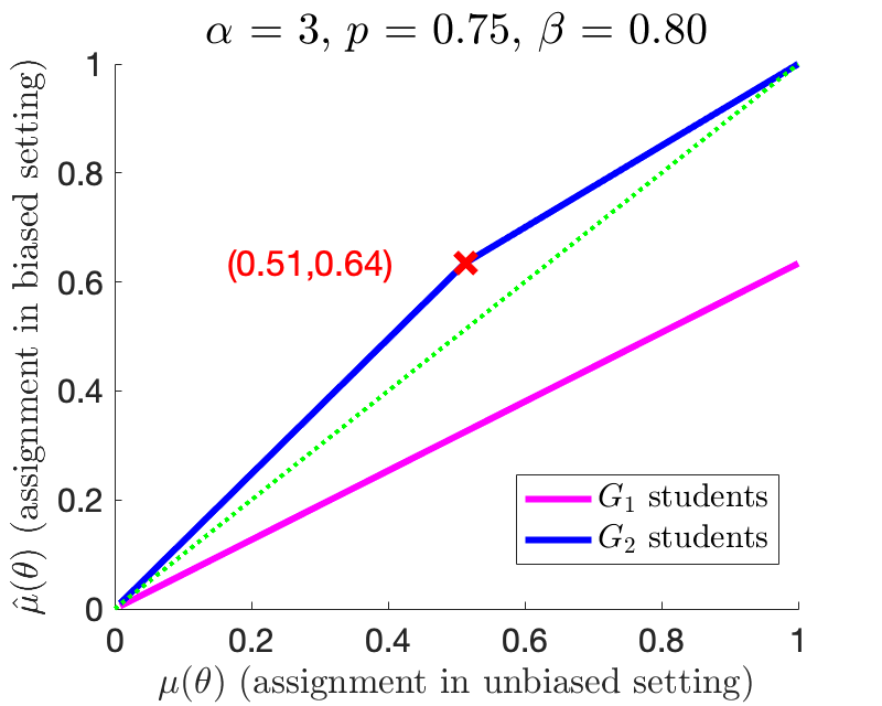
Figure 20: Impact of bias on students when $p>0.5$. Assuming schools are ranked from 0-1, with 0 being the top ranked school, the Y-axis represents the matched schools for the entire student population, when there is bias in evaluations for $G_{2}$ students, and the X-axis represents the matched schools under true potentials.

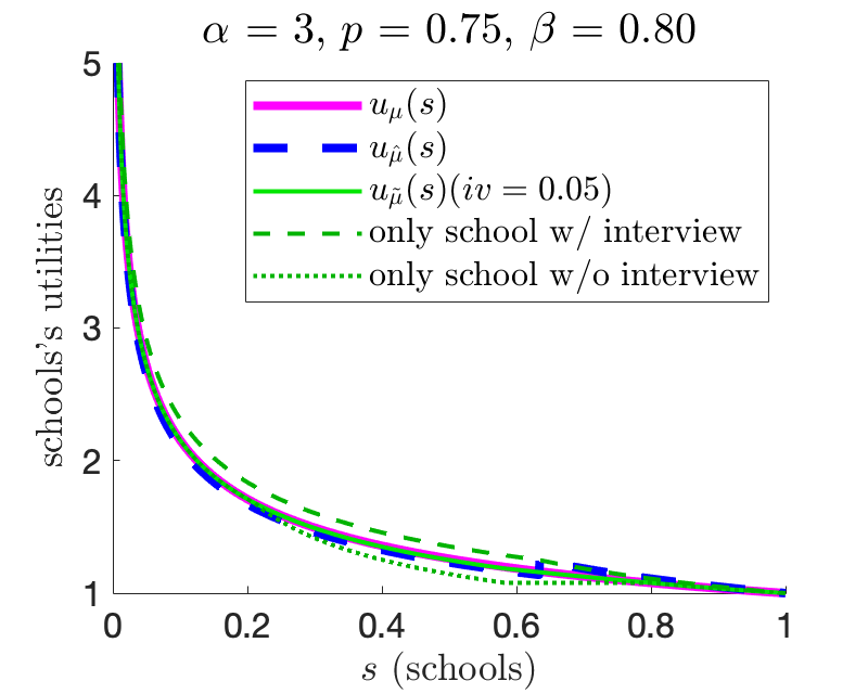
Figure 21: Impact of bias on schools when $p>0.5$.

11 Additional details from Section 6.2

11.1 The Economic Need Index to distinguish $G_{1}$ and $G_{2}$ students

In order to distinguish between $G_{1}$ students and $G_{2}$ students, we make use of another dataset from NYC Open Data (2017), that contain the Economic Need of each school. The dataset contains the Economic Need of each school, measured as the Economic Need Index (ENI), which is a numeric value between 0 and 1 and is used to determine the likelihood that students at the school are in poverty (NYCDOE 2017). Using the median of the ENI as a cutoff point, we deem students from schools whose ENI is higher than the median as $G_{2}$ students and the rest as $G_{1}$ students. Hence, the proportion of $G_{2}$ students is $p=0.50$.

11.2 Empirical analysis of the model

The displacement of students is shown in Figure 22. As in Figure 2, the green dotted line represents the place students should be placed when there is no bias in the system. Displacement for all $G_{1}$ students is non-positive and that for all $G_{2}$ is non-negative. Since $p=0.5$, the benefits experienced by $G_{1}$ students are quite symmetric to the mistreatments experienced by $G_{2}$ students. The deviation of blue and magenta lines from the green dotted line is quite significant, suggesting the necessity of bias-mitigating interventions. Again, we will consider two such strategies: interviewing and vouchers.

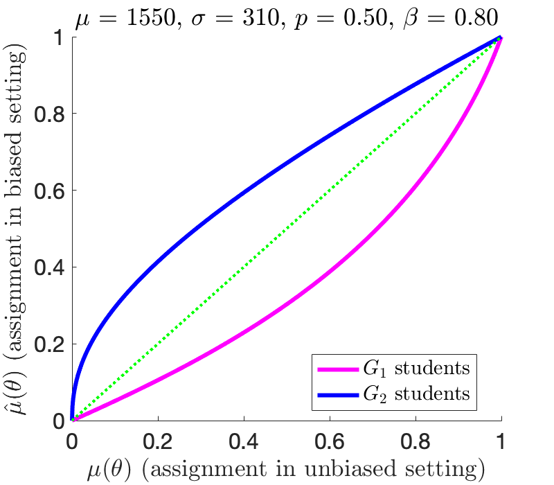
Figure 22: Displacement of students.

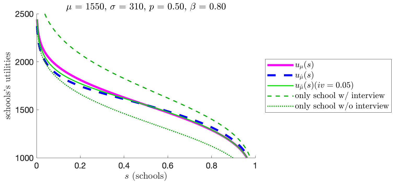
Figure 24: Incentives of conducting interview under normally distributed potentials

A figure similar to Figure 3 is shown in Figure 24 to demonstrate the impact of bias from schools’ perspective for the setting of normally distributed potentials. The utilities of schools in the unbiased setting, $u_{\mu}(s)$, and the utilities of schools in the biased setting, $u_{\widehat{\mu}}(s)$ are not distinctly different. Thus, similarly, bias in the system do not impact schools as significantly as it does for students. In terms of schools’ incentive to conduct interview, again similar to the case of Pareto distribution, although if only one school decides to interview, it has a huge gain in utility, when all schools interview (and interview the same amount of students), the gain of individual school becomes smaller and is longer considerable.

References

- Abdulkadiroğlu et al. (2005) Abdulkadiroğlu A, Pathak PA, Roth AE (2005) The New York City high school match. American Economic Review 95(2):364–367.
- Arnosti (2019) Arnosti N (2019) A continuum model of stable matchings with finite capacities, talk at Simons Institute for the Theory of Computing.
- Ashkenas et al. (2017) Ashkenas J, Park H, Pearce A (2017) Even with affirmative action, blacks and hispanics are more underrepresented at top colleges than 35 years ago. New York Times 1–18.
- Azevedo and Leshno (2016) Azevedo EM, Leshno JD (2016) A supply and demand framework for two-sided matching markets. Journal of Political Economy 124(5):1235–1268.
- Bertsimas et al. (2011) Bertsimas D, Farias VF, Trichakis N (2011) The price of fairness. Operations research 59(1):17–31.
- Biró (2008) Biró P (2008) Student admissions in Hungary as Gale and Shapley envisaged. University of Glasgow Technical Report TR-2008-291 .
- Biró et al. (2010) Biró P, Fleiner T, Irving RW, Manlove DF (2010) The college admissions problem with lower and common quotas. Theoretical Computer Science 411(34-36):3136–3153.
- Boschma and Brownstein (2016) Boschma J, Brownstein R (2016) The concentration of poverty in american schools. The Atlantic 29.
- Burgess et al. (2015) Burgess S, Greaves E, Vignoles A, Wilson D (2015) What parents want: School preferences and school choice. The Economic Journal 125(587):1262–1289.
- Calsamiglia et al. (2010) Calsamiglia C, Haeringer G, Klijn F (2010) Constrained school choice: An experimental study. American Economic Review 100(4):1860–74.
- Celis et al. (2021) Celis LE, Hays C, Mehrotra A, Vishnoi NK (2021) The effect of the rooney rule on implicit bias in the long term. Proceedings of the 2021 ACM Conference on Fairness, Accountability, and Transparency, 678–689.
- Celis et al. (2020) Celis LE, Mehrotra A, Vishnoi NK (2020) Interventions for ranking in the presence of implicit bias. Proceedings of the 2020 Conference on Fairness, Accountability, and Transparency, 369–380.
- Clauset et al. (2009) Clauset A, Shalizi CR, Newman ME (2009) Power-law distributions in empirical data. SIAM review 51(4):661–703.
- College Board (2016) College Board (2016) Total group profile report. https://reports.collegeboard.org/pdf/total-group-2016.pdf.
- Conitzer et al. (2019) Conitzer V, Freeman R, Shah N, Vaughan JW (2019) Group fairness for the allocation of indivisible goods. Proceedings of the 33rd AAAI Conference on Artificial Intelligence (AAAI).
- Corcoran and Baker-Smith (2018) Corcoran SP, Baker-Smith EC (2018) Pathways to an elite education: Application, admission, and matriculation to new york city’s specialized high schools. Education Finance and Policy 13(2):256–279.
- Dwork et al. (2012) Dwork C, Hardt M, Pitassi T, Reingold O, Zemel R (2012) Fairness through awareness. Proceedings of the 3rd Innovations in Theoretical Computer Science conference, 214–226 (ACM).
- Dwork and Ilvento (2018) Dwork C, Ilvento C (2018) Group fairness under composition.
- Education Equity (2020) Education Equity (2020) Equity in SHS. URL http://www.educationequity.nyc.
- Gale and Shapley (1962) Gale D, Shapley LS (1962) College admissions and the stability of marriage. The American Mathematical Monthly 69(1):9–15.
- Gratz v. Bollinger (2003) Gratz v Bollinger (2003) 539 U.S. 244 (2003) https://www.oyez.org/cases/2002/02-516.
- Hafalir et al. (2013) Hafalir IE, Yenmez MB, Yildirim MA (2013) Effective affirmative action in school choice. Theoretical Economics 8(2):325–363.
- Kaggle (2015) Kaggle (2015) Average SAT scores for NYC public schools. https://www.kaggle.com/nycopendata/high-schools.
- Kleinberg et al. (2017) Kleinberg J, Mullainathan S, Raghavan M (2017) Inherent trade-offs in the fair determination of risk scores. 8th Innovations in Theoretical Computer Science Conference (ITCS 2017) (Schloss Dagstuhl-Leibniz-Zentrum fuer Informatik).
- Kleinberg and Raghavan (2018) Kleinberg J, Raghavan M (2018) Selection problems in the presence of implicit bias. arXiv preprint arXiv:1801.03533 .
- Kucsera and Orfield (2014) Kucsera J, Orfield G (2014) New York State’s extreme school segregation: Inequality, inaction and a damaged future .
- Kumar and Kleinberg (2000) Kumar A, Kleinberg J (2000) Fairness measures for resource allocation. Proceedings 41st Annual Symposium on Foundations of Computer Science, 75–85 (IEEE).
- Lovaglia et al. (1998) Lovaglia MJ, Lucas JW, Houser JA, Thye SR, Markovsky B (1998) Status processes and mental ability test scores. American Journal of Sociology 104(1):195–228.
- Luca and Smith (2013) Luca M, Smith J (2013) Salience in quality disclosure: Evidence from the us news college rankings. Journal of Economics & Management Strategy 22(1):58–77.
- Marsh and Schilling (1994) Marsh MT, Schilling DA (1994) Equity measurement in facility location analysis: A review and framework. European Journal of Operational Research 74(1):1–17.
- New York City Department of Education (NYC DOE) New York City Department of Education (NYC DOE) (2019) 2019 NYC High School Directory. https://bigappleacademy.com/wp-content/uploads/2018/06/HSD_2019_ENGLISH_Web.pdf.
- Nguyen and Vohra (2019) Nguyen T, Vohra R (2019) Stable matching with proportionality constraints. Operations Research .
- NYC Open Data (2017) NYC Open Data (2017) 2016 - 2017 school quality report results for high schools. https://data.cityofnewyork.us/Education/2016-2017-School-Quality-Report-Results-for-High-S/ewhs-k7um.
- NYCDOE (2017) NYCDOE (2017) Equity and excellence for all: Diversity in new york city public schools. https://www.schools.nyc.gov/docs/default-source/default-document-library/diversity-in-new-york-city-public-schools-english.
- Quinn Capers et al. (2017) Quinn Capers I, Clinchot D, McDougle L, Greenwald AG (2017) Implicit racial bias in medical school admissions. Academic Medicine 92(3):365–369.
- Roth and Sotomayor (1992) Roth AE, Sotomayor M (1992) Two-sided matching. Handbook of game theory with economic applications 1:485–541.
- Salem and Gupta (2020) Salem J, Gupta S (2020) Closing the gap: Mitigating bias in online résumé-filtering. WINE, 471.
- Sen (1979) Sen A (1979) Equality of what? The Tanner lecture on human values 1.
- Shapiro (2019a) Shapiro E (2019a) Should a single test decide a 4-year-old’s educational future? New York Times .
- Shapiro (2019b) Shapiro E (2019b) Why white parents were at the front of the line for the school tour. New York Times .
- Shapiro (February 06, 2019) Shapiro E (February 06, 2019) Racist? fair? biased? asian-american alumni debate elite high school admissions. The New York Times Magazine .
- Shapiro (March 26, 2019) Shapiro E (March 26, 2019) Segregation has been the story of New York City’s schools for 50 years. The New York Times Magazine .
- Shapiro and Lai (June 03, 2019) Shapiro E, Lai KKR (June 03, 2019) How New York’s elite public schools lost their black and hispanic students. The New York Times Magazine .
- Shapiro and Wang (2019) Shapiro E, Wang V (2019) Amid racial divisions, mayor’s plan to scrap elite school exam fails. New York Times .
- Taube and Linden (1989) Taube KT, Linden KW (1989) State mean sat score as a function of participation rate and other educational and demographic variables. Applied Measurement in Education 2(2):143–159.
- Tomoeda (2018) Tomoeda K (2018) Finding a stable matching under type-specific minimum quotas. Journal of Economic Theory 176:81–117.
- Wikipedia contributors (2019) Wikipedia contributors (2019) List of admission tests to colleges and universities — Wikipedia, the free encyclopedia. https://en.wikipedia.org/w/index.php?title=List_of_admission_tests_to_colleges_and_universities&oldid=914002454, [Online; accessed 9-September-2019].