Power Calculations for Replication Studies

1 Introduction

The replicability of research findings is essential for the credibility of science. However, the scientific world is experiencing a crisis (Begley and Ioannidis,, 2015) as the replicability rate of many fields appears to be alarmingly low. As a result, large scale replication projects, where original studies are selected and replicated as closely as possible to the original procedures, have been conducted in psychology (Open Science Collaboration,, 2015), social sciences (Camerer et al.,, 2018) and economics (Camerer et al.,, 2016) among others. Replication success is usually assessed using significance and $p$-values, compatibility of effect estimates, subjective assessments of replication teams and meta-analysis of effect estimates (e. g. in Open Science Collaboration,, 2015). The statistical evaluation of replication studies is still generating much discussion and new standards are proposed (e. g. in Patil et al.,, 2016; Ly et al.,, 2018; Held,, 2020).

Yet before a replication study is analyzed, it needs to be designed. While the conditions of the replication study are ideally identical to the original study, the replication sample size stands out as an exception and requires further consideration. Using the same sample size as in the original study may lead to a severely underpowered replication study, even if the effect $\hat{\theta}_{o}$ estimated in the original study is the true, unknown effect size $\theta$ (Goodman,, 1992). Standard power calculations using the effect estimate from the original study as the basis for the replication study are commonly used. A major criticism of this method is that the uncertainty accompanying this original finding is ignored and so the resulting replication study is likely to be underpowered (Anderson and Maxwell,, 2017). In this paper, we propose alternatives based on predictive power and adapted from Bayesian approaches to incorporate prior knowledge to sample size calculation in clinical trials (Spiegelhalter et al.,, 2004).

In an era where an increasing number of replication projects are being undertaken, optimal allocation of resources appears to be of particular importance. Adaptive designs are well suited for this purpose and their relevance no longer needs to be justified, particularly in clinical trials where continuing a study which should be stopped can be a matter of life or death. Stopping for futility refers to the termination of a trial when the data at interim indicate that it is unlikely to achieve statistical significance at the end of the trial (Snapinn et al.,, 2006). In contrast, stopping for efficacy arises when the data at interim are so convincing that there is no need to continue collecting more data. One approach for assessing efficacy and futility is called stochastic curtailment (Halperin et al.,, 1982), where the conditional power of the study, given the data so far, is calculated for a range of alternative hypotheses. Instead of conditional power, predictive power can also be used to judge if a trial should be continued (Herson,, 1979). This concept has been discussed in depth in Dallow and Fina, (2011) and Rufibach et al., (2016), with an emphasis on the choice of the prior in the latter.

Lakens, (2014) points out that sequential replication studies could be an alternative to fixed sample size calculations. This approach has been adopted by Camerer et al., (2018) in the Social Science Replication Project (SSRP), a large-scale project aiming at evaluating the replicability of social sciences experiments published between 2010 and 2015 in Nature and Science. A two-stage procedure was used and 21 original studies have been replicated. However, the sequential approach did not include a power calculation at interim, only allowed for a premature stopping for efficacy and did not mention any adjustment on the threshold for significance. We try to fill this gap by proposing different methods to calculate the interim power, namely the power of a replication study taking into account the data from an interim analysis. We argue that predictive interim power is a useful tool to guide the decision to stop replication studies where the intended effect is not present. Our framework only enables power calculation at a single interim analysis.

This paper is structured as follows: power calculations for non-sequential (Section 2) and sequential (Section 3) replication studies are presented, with a focus on comparing conditional and predictive methods. Relevant properties of these methods are then illustrated using data from the SSRP in Section 4. We close with some discussion in Section 5.

2 Non-sequential replication studies

Suppose a study has been conducted in order to estimate an unknown effect size $\theta$. We consider the one-sample case throughout this paper but the results can also be generalized to the case of two samples. The study produced a positive effect estimate $\hat{\theta}_{o}$. In order to confirm this finding, a replication study is planned. Let us assume that the future data of the replication study are normally distributed as follows,

$$Y_{1},\ldots,Y_{n_{r}}\mathrel{\overset{\text{iid}}{\thicksim}}\operatorname{N}\left(\theta,\sigma^{2}\right)\,,$$

where $\sigma$ is the known standard deviation of one observation, assumed to be the same for original and replication study. In the SSRP, as well as in most replication projects, power calculations for the replication studies are based on the original effect estimate $\hat{\theta}_{o}$. In order to incorporate the uncertainty of $\hat{\theta}_{o}$ we use the following prior

$$\theta\sim\operatorname{N}\left(\hat{\theta}_{o},\sigma^{2}_{o}=\sigma^{2}/n_{o}\right)\,,$$ (1)

centered around $\hat{\theta}_{o}$ and with variance inversely proportional to the original sample size $n_{o}$ (Spiegelhalter et al.,, 2004). Prior (1) may be too optimistic in practice, where original effect estimates tend to be exaggerated (Camerer et al.,, 2018). This issue and possible solutions are discussed in the next section.

In what follows, the different formulas resulting from the use of the prior (1) are described. This section is inspired by Section 6.5 in Spiegelhalter et al., (2004) where Bayesian contributions to selecting the sample size of a clinical trial are studied. We adapt this methodology to the replication framework and express the power calculation formulas in terms of unitless quantities (namely relative sample sizes and test statistics).

2.1 Methods

We differentiate between design and analysis prior, both having an impact on the power calculation (O’Hagan and Stevens,, 2001), and present the different combinations of priors in Table 1.

Table 1: Methods of power calculations resulting from the different combinations of design and analysis priors.

		Design
		Point prior $\theta=\hat{\theta}_{o}$	Normal prior $\theta\sim\operatorname{N}\left(\hat{\theta}_{o},\sigma^{2}_{o}\right)$
Analysis	Flat prior	blablablablablablablablablablabl Conditional blablablablablablablablablablabl	Predictive
	Normal prior $\theta\sim\operatorname{N}\left(\hat{\theta}_{o},\sigma^{2}_{o}\right)$	blablablablablablablablablablabl Conditional Bayesian blablablablablablablablablablabl	Fully Bayesian

A point prior at $\theta=\hat{\theta}_{o}$ in the design corresponds to the concept of conditional power (Spiegelhalter and Freedman,, 1986). In contrast, the normal design prior (1) is related to the concept of predictive power, which averages the conditional power over the possible values of the true effect according to its design prior distribution. Alternative names in the literature are assurance (O’Hagan et al.,, 2005), probability of study success (Wang et al.,, 2013) and Bayesian predictive power (Spiegelhalter et al.,, 1986). Conditional and predictive power are usually accompanied by a flat analysis prior, but can also be calculated assuming that original and replication data are pooled (using the normal analysis prior (1)), resulting in the conditional Bayesian power and the fully Bayesian power, respectively.

In practice, publication bias and the winner’s curse often lead to overestimated original effect estimates (Ioannidis,, 2008; Button et al.,, 2013; Anderson and Maxwell,, 2017). Hence, prior (1) might be over-optimistic and lead to underpowered replication studies. A simple way to correct for this over-optimism is to multiply the design prior mean $\hat{\theta}_{o}$ in (1) by a factor $d$ between $0$ and $1$. The corresponding shrinkage factor $s=1-d$ can be chosen based on previous replication studies in the same field. This is the approach considered in the SSRP and we expand on this in Section 4. More advanced methods using empirical Bayes based power estimation (Jiang and Yu,, 2016) and data-driven shrinkage (Pawel and Held,, 2020) are not considered here.

2.1.1 Conditional power

Conditional power is the probability that a replication study will lead to a statistically significant conclusion at the two-sided level $\alpha$, given that the alternative hypothesis is true (Spiegelhalter et al.,, 2004, Section 2.5). In the context of a replication study, the alternative hypothesis is represented by the effect estimate $\hat{\theta}_{o}$ from the original study.

Let $z_{\alpha/2}$ and $\Phi[\cdot]$ respectively denote the $\alpha/2$-quantile and the cumulative distribution function of the standard normal distribution. The conditional power of a replication study with sample size $n_{r}$ is

$$\text{CP}=\Phi\left[\frac{\hat{\theta}_{o}\sqrt{n_{r}}}{\sigma}+z_{\alpha/2}\right]\,,$$ (2)

see Appendix A.1 for a derivation. The required replication sample size $n_{r}$ can be obtained by rearranging (2).

A key feature of our framework is that all power/sample size formulas are expressed without absolute effect measures. Simple mathematical rearrangements produce an expression which only depends on the original test statistic $t_{o}=\hat{\theta}_{o}/\sigma_{o}=\hat{\theta}_{o}\sqrt{n_{o}}/\sigma$ and the variance ratio $c=\sigma^{2}_{o}/\sigma^{2}_{r}$ which simplifies to the relative sample size $c=n_{r}/n_{o}$ and represents how much the sample size in the replication study is increased as compared to the one in the original study. Formula (2) then becomes

CP $$=\Phi\left[\sqrt{c}\,t_{o}+z_{\alpha/2}\right]\,.$$ (3)

This formula highlights an intuitive property of the conditional power: the larger the evidence in the original study (quantified by $t_{o}$) or the larger the increase in sample size compared to the original study (represented by $c$), the larger the conditional power of the replication study.

2.1.2 Predictive power

In order to incorporate the uncertainty of $\hat{\theta}_{o}$, the concept of predictive power is discussed (Spiegelhalter and Freedman,, 1986). Its formula is:

$$\text{PP}=\Phi\left[\sqrt{\frac{n_{o}}{n_{o}+n_{r}}}\left(\frac{\hat{\theta}_{o}\sqrt{n_{r}}}{\sigma}+z_{\alpha/2}\right)\right]\,,$$ (4)

see Appendix A.2 for a derivation. The predictive power (4) tends to the conditional power (3) as the original sample size $n_{o}$ increases. Using the unitless quantities $t_{o}$ and $c$, the predictive power can be rewritten as

PP $$=\Phi\left[\sqrt{\frac{c}{c+1}}\,t_{o}+\sqrt{\frac{1}{c+1}}\,z_{\alpha/2}\right]\,.$$ (5)

2.1.3 Fully Bayesian and conditional Bayesian power

So far two power calculation methods where a flat analysis prior is used have been considered. This approach corresponds to the two-trials rule in drug development, which requires “at least two adequate and well-controlled studies, each convincing on its own, to establish effectiveness” (FDA,, 1998, p. 3). In practice, this translates to two studies with a significant $p$-value and an effect in the intended direction.

An alternative approach for the analysis is to pool original and replication data. This is similar to a meta-analysis of original and replication effect estimates, as done in the SSRP for example. However, in order to ensure the same evidence level as when original and replication studies are analyzed independently, the corresponding two-sided significance level $\tilde{\alpha}=\alpha^{2}/2$ should be used (Fisher,, 1999; Gibson,, 2020).

The fully Bayesian power is calculated using the prior (1) in both the design and the analysis. Using the same prior beliefs in both stages is considered as the most natural approach by some authors (e. g. in O’Hagan and Stevens,, 2001). The corresponding formula is

$$\text{FBP}=\Phi\left[\sqrt{\frac{c+1}{c}}\,t_{o}+\sqrt{\frac{1}{c}}\,z_{\tilde{\alpha}/2}\right]\,.$$ (6)

Note that the fully Bayesian power is also a predictive power as it incorporates the uncertainty of the original effect estimate $\hat{\theta}_{o}$.

The last possible combination of design and analysis priors leads to the conditional Bayesian power:

$$\text{CBP}=\Phi\left[\frac{c+1}{\sqrt{c}}\,t_{o}+\sqrt{\frac{c+1}{c}}\,z_{\tilde{\alpha}/2}\right]\,.$$ (7)

Derivations of (6) and (7) can be found in Appendix A.4 and A.3.

2.2 Properties

For fixed relative sample size $c$ and two-sided level $\alpha$, all four formulas (3), (5), (6) and (7) react to an increase in original test statistic $t_{o}$ with a monotone increase in power. However, the original result cannot be changed and it is more realistic to study the power when varying the relative sample size $c$ for fixed original test statistic $t_{o}$ instead. Consider two original studies with $p$-values $0.046$ and $0.005$. These $p$-values correspond to the original studies by Duncan et al., (2012) and Shah et al., (2012) in the SSRP dataset and are used in the following for illustrative purposes.

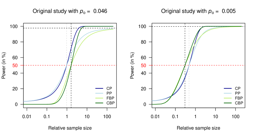
Figure 1: CP, PP, FBP and CBP as a function of the relative sample size $c$ for two original studies with $p_{o}=0.046$ (left) and $p_{o}=0.005$ (right) at the two-sided $\alpha=5$% level, so $\tilde{\alpha}=0.00125$. The vertical grey line corresponds to the intersection of CP and PP curves as calculated in (8), and the vertical black line to the intersection of FBP and CBP as in (9). The horizontal black line indicates the asymptote $1-p_{o}/2$ of PP and FBP.

2.2.1 Conditional vs. predictive power

The power obtained with predictive methods is always closer to 50% than the power obtained with conditional methods (Spiegelhalter et al.,, 2004; Grouin et al.,, 2007; Dallow and Fina,, 2011). In practice, power is typically larger than 50% and this implies that CP (3) is larger than PP (5); and CBP (7) is larger than FBP (6).

Furthermore, it can be shown that CP and PP are both equal to 50% if the relative sample size is

$$c=z_{\alpha/2}^{2}/t_{o}^{2}\,,$$ (8)

the squared $\alpha/2$-quantile of the normal distribution divided by the squared test statistic from the original study (see Appendix A.5 for details). Equation (8) implies that the larger the evidence in the original study (quantified by $t_{o}$), the smaller the relative sample size $c$ where CP and PP curves intersect.

This can be observed in Figure 1, where the relative sample size at the intersection of the CP and PP curves is closer to zero in the replication of a convincing original study ($p_{o}=0.005$, $c=0.48$) than in the replication of a borderline original study ($p_{o}=0.046$, $c=0.96$). Likewise, FBP and CBP are crossing at a power of 50% with corresponding relative sample size

$$c=z_{\tilde{\alpha}/2}^{2}/t_{o}^{2}-1\,.$$ (9)

2.2.2 Predictive power cannot always reach 100%

Unlike CP (3) which always reaches 100% for a sufficiently large replication sample size, PP (5) has an asymptote at $1-p_{o}/2$. This means that the more convincing the original study, the closer to 100% the PP of an infinitely large replication study is. In a sense, the original result penalizes the predictive power. However, this penalty is not very stringent, as replication of an original study with a two-sided $p$-value of 0.05 would still be able to reach a PP of 97.5% for a sufficiently large replication sample size. This property also applies to the FBP and can be observed in Figure 1 where the horizontal black line indicates the asymptote $1-p_{o}/2$.

2.2.3 Pooling original and replication studies

For a borderline significant original study (e.g. $p_{o}=0.046$ in Figure 1), FBP (6) and CBP (7) are respectively always smaller than PP (5) and CP (3). In contrast, when the original study is more convincing (e.g. $p_{o}=0.005$ in Figure 1), FBP is larger than PP (respectively CBP larger than CP) for some values of $c$. However, if $p_{o}<\tilde{\alpha}$, the level required at the end of the replication study (typically $\tilde{\alpha}=0.00125$), FBP and CBP converge to 100% for $c\to 0$, decrease down to

$$\Phi\left[\sqrt{t_{o}^{2}-z_{\tilde{\alpha}/2}^{2}}\,\right]$$ (10)

for increasing $c$ and then increase to $1-p_{o}/2$ (FBP) or 100% (CBP). See Appendix A.6 for a derivation. A highly convincing original study will thus always have FBP and CBP very close to 100% independently of the sample size. This implies that a replication may not be required at all, a clear disadvantage of pooling original and replication studies instead of considering them independently.

3 Sequential replication studies

In Section 2, power calculations are performed before any data have been collected in the replication study. This framework is extended in this section and allows power (re)calculation at an interim analysis, after some data have been collected in the replication study already. The interim power is defined as the probability of statistical significance at the end of the replication study given the data collected so far. The incorporation of prior knowledge into interim power has been studied in Spiegelhalter et al., (2004, Section 6.6) and we adapt this approach to the case where prior information refers to a single original study. Moreover, the power calculation formulas are expressed in terms of unitless quantities (relative sample sizes and test statistics) in the following. It is well known from the field of clinical trials that the maximum sample size (if the trial has not been stopped at interim) increases with the number of planned interim analyses (Matthews,, 2006, Section 8.2.1). In order to maintain a given power, even one interim analysis requires a larger maximum sample size than for a trial with a fixed size and the calculation of the replication sample size should take this into account.

3.1 Methods

In addition to the point prior $\theta=\hat{\theta}_{o}$ and the normal prior (1), the new framework enables the specification of a flat design prior. Table 2 shows the different types of interim power calculations that are investigated in this section.

Table 2: Methods of interim power calculations resulting from different design priors using a flat analysis prior.

Design
Point prior $\theta=\hat{\theta}_{o}$	Normal prior $\theta\sim\operatorname{N}\left(\hat{\theta}_{o},\sigma^{2}_{o}\right)$	Flat prior
blablablablablablablablablablabl Conditional blablablablablablablablablablabl	Informed predictive	Predictive

Calculating the interim power to detect the effect estimate from the original study ignores the uncertainty of the original result. This corresponds to the conditional power in Table 2. Uncertainty of the original result can be taken into account when recalculating the power at an interim analysis, turning the conditional power into a predictive power. This requires the selection of a prior distribution for the true effect, which is updated by the data collected so far in the replication study. The prior distributions discussed here are the normal prior (1) (leading to the informed predictive power) and a flat prior (leading to the predictive power). The conditional power is then averaged with respect to the posterior distribution of the true effect size, given the data already observed in the replication study. A pooled analysis of original and replication data can also be considered in this framework but is omitted here.

Let $\hat{\theta}_{i}$ be the effect estimate at interim and $\sigma^{2}_{i}=\sigma^{2}/n_{i}$ the corresponding variance, with $n_{i}$ the sample size at interim. The sample size that is still to be collected in the replication study is denoted by $n_{j}$ and the total replication sample size is thus $n_{r}=n_{i}+n_{j}$. The interim power formulas can be shown to only depend on the original and interim test statistics $t_{o}$ and $t_{i}=\hat{\theta}_{i}/\sigma_{i}$, the relative sample size $c=n_{r}/n_{o}$ and the variance ratio $f=\sigma^{2}_{r}/\sigma^{2}_{i}=n_{i}/n_{r}$, the fraction of the replication study already completed.

3.1.1 Conditional power at interim

The conditional power at interim is the interim power to detect the effect $\theta=\hat{\theta}_{o}$. It can be expressed as

CPi $$=\Phi\left[\sqrt{c(1-f)}\,t_{o}+\sqrt{\frac{f}{1-f}}\,t_{i}+\sqrt{\frac{1}{1-f}}\,z_{\alpha/2}\right]\,,$$ (11)

see Appendix B.1 for a derivation. In the particular case where no data has been collected yet in the replication study ($f=0$), the CPi (11) reduces to the CP (3). Interim power can also be calculated to detect $\theta=\hat{\theta}_{i}$, this is however not recommended (Bauer and König,, 2006; Kunzmann et al.,, 2020).

3.1.2 Informed predictive power at interim

The informed predictive power at interim is the predictive interim power using the design prior (1). It can be formulated as

IPPi $$=\Phi\left[\sqrt{\frac{c(1-f)}{(cf+1)(1+c)}}\,t_{o}+\sqrt{\frac{f(1+c)}{(1-f)(cf+1)}}\,t_{i}+\sqrt{\frac{cf+1}{(1+c)(1-f)}}\,z_{\alpha/2}\right]\,,$$ (12)

see Appendix B.2 for a derivation. In the case of $f=0$ (no data collected in the replication study so far), the IPPi (12) reduces to the PP (5). By considering the original result but also its uncertainty, the predictive power at interim is a compromise between considering only the original effect estimate (CPi) and ignoring the original study completely (PPi).

3.1.3 Predictive power at interim

The predictive power at interim is the predictive interim power using a flat design prior. In other words, the results from the original study are ignored. It is expressed as

PPi $$=\Phi\left[\sqrt{\frac{1}{1-f}}\,t_{i}+\sqrt{\frac{f}{1-f}}\,z_{\alpha/2}\right]\,,$$ (13)

see Appendix B.3 for a derivation. Note that PPi (13) corresponds to FBP (6) provided that the original study in FBP formula is considered as the interim study (see Appendix B.3). This illustrates the dependence of original and replication studies when a normal prior is used in the analysis.

3.2 Properties

Theoretical and specific properties of the conditional, informed predictive and predictive power at interim are discussed.

3.2.1 Conditional vs  predictive power

The power at interim, as compared to study start, involves two additional parameters, namely the test statistic $t_{i}$ from the interim analysis and the fraction $f$ of the replication study already conducted. It is therefore not straightforward to compare the different methods in terms of which one results in a larger power. Comparison is facilitated if certain assumptions are made. Consider any combination of a significant original result, a non-significant interim result and a replication sample size at least twice as large as the original sample size. This translates to $t_{o}>z_{1-\alpha/2}$, $t_{i}<z_{1-\alpha/2}$ and $c\geq 2$ in formulas (11), (12) and (13). Under these assumptions and with $f>0.25$, the CPi is always larger than the IPPi, which is always larger than the PPi, see Appendix B.4. However, one has to be careful as these conditions are sufficient, but not necessary for obtaining this order.

3.2.2 Weights given to original and interim results

Equations (11), (12) and (13) can be expressed as $\Phi[x]$ where $x$ is a weighted average of $t_{o}$, $t_{i}$ and $z_{\alpha/2}$ with weights $w_{o}$, $w_{i}$ and $w_{\alpha}$, say. The weights $w_{o}$ and $w_{i}$ depend on the relative sample size $c$ and the fraction $f$ of the replication study already completed.

In the CPi formula (11), an increase in $c$ leads to a monotone increase in $w_{o}$ and does not affect $w_{i}$. In other words, the weight given to the original result in the CPi becomes larger if the relative sample size $c$ increases. Furthermore, the larger the fraction $f$ of the replication study already completed, the less weight is given to the original result and conversely, the more weight to the interim result.

In the IPPi formula (12), an increase in $f$ leads to a decrease in $w_{o}$ and an increase in $w_{i}$. Only if the interim analysis takes place early will the original result have a greater weight than the interim result in the calculation of the IPPi, see Appendix B.5.

In the PPi formula (13), no weight is given to the original result and the weight $w_{i}$ given to interim results increases when $f$ increases.

3.2.3 A power of 100% cannot always be reached with the predictive methods

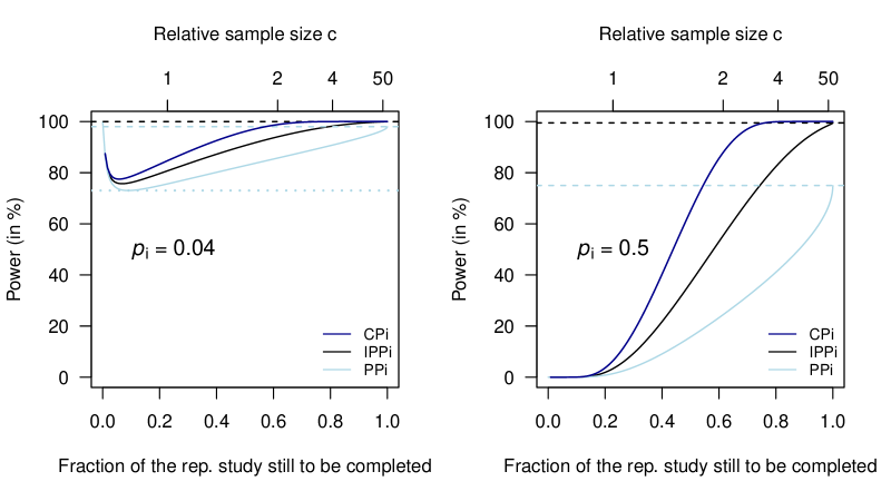
Figure 2: CPi, IPPi and PPi as a function of the sample size $n_{j}$ still to be collected in the replication study (or equivalently, as a function of the fraction of the replication study still to be completed ($1-f$) and the relative sample size $c$) for an original study with $p_{o}=0.005$ and with two hypothetical interim $p$-values $p_{i}=0.04$ (left) and $p_{i}=0.5$ (right). The two-sided level $\alpha$ is $0.05$. Horizontal dashed lines represent the asymptotes of IPPi and PPi and the horizontal dotted line represents the minimum PPi.

Considering that an interim analysis has been conducted, $n_{i}$ and $t_{i}$ are fixed, and the only parameter that can vary is the sample size $n_{j}$ still to be collected in the replication study. Increasing this sample size results in an increase of the relative sample size $c$ and a decrease of the fraction $f$ of the replication study already completed. If $n_{j}$ is large enough, the CPi (11) reaches 100%. In contrast, the asymptotes of IPPi (12) and PPi (13) are penalized by the original and/or interim results. The larger the evidence in the original study and at interim (represented by $t_{o}$ and $t_{i}$, respectively), the larger the asymptote of the IPPi (formula given in Appendix B.6). The asymptote of the PPi, on the other hand, is $1-p_{i}/2$. This last property is explained in Dallow and Fina, (2011, Section 4) and the asymptotes can be visualized in Figure 2 for an original study with $p_{o}=0.005$ and two hypothetical interim results: $p_{i}=0.04$ and $p_{i}=0.5$. On the left panel, the asymptotes of CPi, IPPi and PPi are all close to 100% as original and interim $p$-values are fairly small. A large increase in interim $p$-value hardly has an effect on the asymptote of the IPPi (from $99.98$% to $99.5$%, right panel) but results in a dramatic decrease of the asymptote of the PPi and remarkably, the maximum PPi achievable for a study with an interim $p$-value of 0.5 is only $75$%.

3.2.4 Non-monotonicity property of power

If the two-sided interim $p$-value is not significant ($p_{i}>\alpha$), the interim power with all three methods behaves in an expected way: it increases with increasing sample size $n_{j}$. However, this property breaks when $p_{i}<\alpha$. In this situation, the power assuming no additional subject to be added ($f=1$) is 100%, declines with increasing $n_{j}$ (decreasing $f$) and then increases. For example, the minimum predictive power at interim can be shown to be $\Phi\left[\sqrt{t_{i}^{2}-z_{\alpha/2}^{2}}\,\right]$ which means that the PPi of any replication study with a significant interim result will never be smaller than 50% (details in Appendix B.7). This property can be observed in Figure 2 (left panel) where the PPi cannot be smaller than $73\%$. Dallow and Fina, (2011) explain this characteristic as follows: “Intuitively, if the interim results are very good, any additional subject can be seen as a potential threat, able to damage the current results rather than a resource providing more power to our analysis.”

4 Application

Twenty-one significant original findings were replicated in the SSRP and a two-stage procedure was adopted. In stage 1, the replication studies had 90% power to detect 75% of the original effect estimate. Data collection was stopped if a two-sided $p$-value $<0.05$ and an effect in the same direction as the original effect were found. If not, data collection was continued in stage 2 to have 90% power to detect 50% of the original effect estimate for the first and second data collections pooled. The shrinkage factor $s$ was chosen to be 0.5 as a previous replication project in the psychological field (Open Science Collaboration,, 2015) found replication effect estimates on average half the size of the original effect estimates. Stages 1 and 2 can be considered as two steps of a sequential analysis, with an interim analysis in between. The analysis after stage 1 will be called the interim analysis while the final analysis will refer to the analysis based on the pooled data from stages 1 and 2.

The complete SSRP dataset with extended information is available at https://osf.io/pfdyw/. The effects are given as correlation coefficients, making them easily interpretable and comparable. Moreover, the application of Fisher’s $z$ transformation $z(r)=\tanh^{-1}(r)$ to the correlation coefficients justifies an asymptotic normal distribution and the standard error of the transformed coefficients becomes a function of the effective sample size $n-3$ only, $\operatorname{se}(z)=1/\sqrt{n-3}$. In this dataset, original effects are always positive. A ready-to-use dataset SSRP can be found in the package ReplicationSuccess, available at https://r-forge.r-project.org/projects/replication/.

4.1 Descriptive results

The results are displayed in Figure 3. Twelve studies were significant at interim with an effect in the correct direction but by mistake only eleven were stopped. Out of the ten studies that were continued, only two showed a significant result in the correct direction at the final analysis. The study that was wrongly continued turned out to be non-significant at the final analysis. The effect of publication bias is clearly seen: original effect estimates are larger than the corresponding replication effect estimates for 19 out of the 21 studies and are on average twice as large.

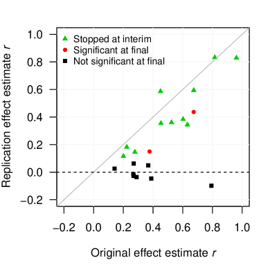
Figure 3: Original effect estimate vs. replication effect estimate (on the correlation scale). Replications which were not pursued in stage 2 are included with the results from stage 1. Shape and color of the point indicate whether the study was stopped due to a significant result in the correct direction at interim (green triangle), was significant in the correct direction at the final analysis (red circle) or was not significant at the final analysis (black square). The diagonal line indicates replication effect estimates equal to original effect estimates.

4.2 Power calculations

The methods described in Sections 2 and 3 are used to calculate the power of the 21 replication studies before the onset of the study and at the interim analysis. Because our calculations are based on Fisher’s $z$-transformed correlation coefficients, the effective sample sizes are used. The relative sample size is then $c=(n_{r}-3)/(n_{o}-3)$ and the fraction $f$ of the replication study already completed $f=(n_{i}-3)/(n_{r}-3)$. A two-sided $\alpha=5$% level is used as in the original paper, so $\tilde{\alpha}=0.00125$ in the calculation of FBP and CBP.

4.2.1 At the replication study start

We computed the CP, PP, FBP and CBP of the 21 replication studies. The replication sample size that we considered in the calculations is the one used by the authors of the SSRP in stage 1, ignoring stage 2. To be consistent with the procedures of the SSRP, a shrinkage factor $s$ of 0.25 was used in the calculations. Results can be found in Figure 4, where some properties discussed in Section 2.2 are illustrated. CP is larger than PP for all studies, and similarly CBP is larger than FBP as expected (see Section 2.2.1). Furthermore, it can be oberved that for some studies FBP is larger than PP, while it is the opposite for some other studies. This depends on the $p$-value $p_{o}$ from the original study and the relative sample size $c$ as explained in Section 2.2.3. The same applies to CP and CBP but cannot be directly observed in Figure 4.

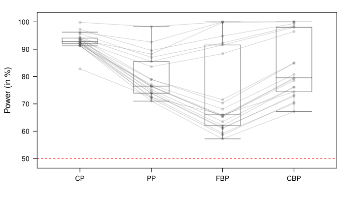
Figure 4: CP, PP, FBP and CBP of the 21 studies of the SSRP at level $\alpha=5\%$ (so $\tilde{\alpha}=0.00125$ for FBP and CBP) using a shrinkage factor $s$ of 0.25 in the calculations. Each circle represents a study and the lines link the same studies.

4.2.2 At the interim analysis

Replication studies which did not reach significance after the first data collection were continued. We have selected these studies and calculated their interim power with the different methods (see Table 3). These studies have a sample size substantially larger in the replication as compared to the original study (large $c$). Moreover, the interim analysis took place in the second quarter of the replication study ($0.3\leq f\leq 0.47)$ and by selection, they all have a non-significant interim $p$-value (except the study from Ackerman et al., (2010) which was continued by mistake). Excluding this study, they all fulfill the sufficient conditions mentioned in Section 3.2.1 and follow the order CPi > IPPi > PPi. This also hold for the particular study with a significant interim result as the corresponding relative sample size $c$ is large ($c=11.62$).

The CPi is remarkably large for all studies, even for the five studies where the interim effect estimate is in the opposite direction as the original estimate as the weight given to the significant original result is consequent due to the large relative sample size $c$ (see Section 3.2.2). In contrast, more weight is given to the interim as compared to the original result in the IPPi formula, making the corresponding IPPi values more sensible. If a futility boundary between 10% and 30% had been used (as in DeMets, (2006)) four out of the eight studies which failed to replicate at the final analysis would have been stopped at interim based on the IPPi values. Surprisingly, the replication study of Ramirez and Beilock, (2011) presents a relatively large IPPi ($61.4$%) although the interim result goes in the opposite direction as the original result. This is due to the very small original $p$-value. The PPi of the same study is considerably smaller ($4.2$%) since the original result does not influence the power with this method. Furthermore, six out of eight studies which failed to replicate at the final analysis would have been stopped at interim if futility stopping had been decided based on a PPi of less than 30%. Significant interim results lead to large PPi values (see Section 3.2.4), and that can observed for the study that was incorrectly continued.

Table 3: CPi, IPPi and PPi of the ten studies that were continued including the original, interim and replication two-sided $p$-values and effect estimates, the relative sample size $c$ and the fraction $f$ of the replication study already completed.

	Original		Interim			Interim power			Replication
Study	$p_{o}$	$r_{o}$	$f$	$p_{i}$	$r_{i}$	CPi	IPPi	PPi	$c$	$p_{r}$	$r_{r}$
Duncan	0.005	0.67	0.37	0.29	0.18	100.0	74.6	43.4	7.42	0.00001	0.44
Pyc	0.023	0.38	0.43	0.09	0.15	100.0	85.3	71.0	9.18	0.009	0.15
Ackerman	0.048	0.27	0.43	0.02	0.14	100.0	95.0	90.3	11.69	0.125	0.06
Rand	0.009	0.14	0.47	0.37	0.03	99.8	51.9	27.0	6.27	0.234	0.03
Ramirez	0.000008	0.79	0.30	0.72	-0.08	100.0	61.4	4.2	4.47	0.390	-0.10
Gervais	0.029	0.29	0.42	0.41	-0.05	97.5	1.9	0.3	9.78	0.415	-0.04
Lee	0.013	0.39	0.42	0.45	-0.07	97.7	3.1	0.4	7.65	0.435	-0.05
Sparrow	0.002	0.37	0.44	0.27	0.11	99.7	74.1	40.1	3.50	0.451	0.05
Kidd	0.012	0.27	0.40	0.27	-0.07	98.9	1.6	0.1	8.57	0.467	-0.03
Shah	0.046	0.27	0.45	0.15	-0.09	87.0	0.1	0.0	11.62	0.710	-0.02

5 Discussion

Conditional power calculations appear to be the norm in most replication projects. In this paper, we have drawn attention to notable shortcomings of this approach and outlined the rationale and properties of predictive power. We encourage researchers to abandon conditional methods in favor of predictive methods which make a better use of the original study and its uncertainty.

Furthermore, as many replications are being conducted and only a fraction confirms the original result, we argue for the necessity of sequentially analyzing the results. With this in mind, we encourage the initiative from Camerer et al., (2018) to terminate some replication studies prematurely based on an interim analysis. However, their approach only enables efficacy stopping. We propose to use interim power to judge if a replication study should be stopped for futility. Interim analyses can help to save time and resources but also raise new questions with regard to the choice of prior distributions. We have shown using studies from the SSRP that different design priors lead to very different power values and by extension to different decisions. Conditioning the power calculations at interim on the original results is even more unreasonable than at the study start and leads to very large power values given a significant original result, even if interim results suggest evidence in the opposite direction. We recommend the use of IPPi and PPi to make futility decisions. A 30% futility boundary is sometimes employed in clinical trials and has proved to be reasonable in the SSRP. Efficacy stopping based on interim power is known to inflate the type-I error rate (Jennison and Turnbull,, 1999, Chapter 10). We only consider futility stopping as this issue does not apply here (Lachin,, 2005).

Some limitations should be noted. First, the paper discusses power calculations before the onset of the study and at an interim analysis separately. However, the planned interim analysis has an impact on power at study start and sample size adjustments are necessary (Wassmer and Brannath,, 2016, Section 2.1.2). This is nevertheless rarely done in current replication projects such as SSRP. Second, while the ICH E9 ‘Statistical Principles for Clinical Trials’ (ICH E9 Expert Working Group,, 1999) recommends blinded interim results, our data at interim are assumed to be unblinded. This is not a problem for the one-sample case but becomes an issue when we want to compare two groups. Such a situation would require an Independent Data Monitoring Committee to prevent the replication study from being biased (Kieser and Friede,, 2003). Third, the assumption of normally distributed observations is made.

Further research will focus on extending this framework to multiple interim analyses in a replication study and to sequentially conducted replication studies. It will also be of interest to apply the concept of interim power discussed in Section 3 to the reverse-Bayes assessment of replication success (Held,, 2020).

Software

Software for these power calculations can be found in the R-package
ReplicationSuccess, available at https://r-forge.r-project.org/projects/replication/. An example of the usage of this package is given in Appendix C.

Appendix A Non-sequential replication study

A.1 Conditional power (CP)

Let the sample mean of $Y_{1:n_{r}}$ be the parameter estimate of the replication study with distribution

$$\vbox{\hrule height=0.5pt\kern 2.15277pt\hbox{\kern-1.00006pt$Y$\kern-1.00006pt}}_{n_{r}}\sim\operatorname{N}\left(\theta,\sigma^{2}/n_{r}\right)\,.$$ (14)

Let us suppose the null hypothesis of the replication study is $H_{0}$: $\theta=0$ and we want to detect an alternative hypothesis $H_{1}$: $\theta=\hat{\theta}_{o}>0$, where $\hat{\theta}_{o}$ is the effect estimate of the original study. The corresponding standardized test statistic $t_{r}$ is $\vbox{\hrule height=0.5pt\kern 2.15277pt\hbox{\kern-1.00006pt$Y$\kern-1.00006pt}}_{n_{r}}\sqrt{n_{r}}/\sigma$ and we declare the result statistically significant at the two-sided level $\alpha$ if $\left\lvert t_{r}\right\rvert>z_{1-\alpha/2}=-z_{\alpha/2}$. In the following, we focus on $t_{r}>-z_{\alpha/2}$ as $\Pr\left(t_{r}<z_{\alpha/2}\right)$ is relatively small for $\hat{\theta}_{o}>0$.

$H_{0}$ is rejected if

$$\vbox{\hrule height=0.5pt\kern 2.15277pt\hbox{\kern-1.00006pt$Y$\kern-1.00006pt}}_{n_{r}}>-\frac{1}{\sqrt{n_{r}}}z_{\alpha/2}\sigma\,.$$

Following notation from Spiegelhalter et al., (2004, Section 6.5.2), this event is denoted by $S^{C}_{\alpha/2}$. The conditional power can be expressed as

$$\Pr\left(S^{C}_{\alpha/2}\,|\,\theta\right) =\Pr\left(\vbox{\hrule height=0.5pt\kern 2.15277pt\hbox{\kern-1.00006pt$Y$\kern-1.00006pt}}_{n_{r}}>-\frac{1}{\sqrt{n_{r}}}z_{\alpha/2}\sigma\right)$$

$$=\Phi\left[\frac{\theta\sqrt{n_{r}}}{\sigma}+z_{\alpha/2}\right]\,.$$ (15)

Setting $\theta=\hat{\theta}_{o}$ in (15) gives the CP formula (2).

A.2 Predictive power (PP)

Predictive power is computed by integrating (15) with respect to the prior (1). Integration can be demanding and a more direct way is to use the predictive distribution of $\vbox{\hrule height=0.5pt\kern 2.15277pt\hbox{\kern-1.00006pt$Y$\kern-1.00006pt}}_{n_{r}}$,

$$\vbox{\hrule height=0.5pt\kern 2.15277pt\hbox{\kern-1.00006pt$Y$\kern-1.00006pt}}_{n_{r}}\sim\operatorname{N}\left(\hat{\theta}_{o},\sigma^{2}\left(1/n_{o}+1/n_{r}\right)\right)\,,$$ (16)

obtained by combining the prior (1) and the likelihood (14). The predictive power is

$$\Pr\left(S^{C}_{\alpha/2}\right) =\Pr\left(\vbox{\hrule height=0.5pt\kern 2.15277pt\hbox{\kern-1.00006pt$Y$\kern-1.00006pt}}_{n_{r}}>-\frac{1}{\sqrt{n_{r}}}z_{\alpha/2}\sigma\right)$$

$$=\Phi\left[\sqrt{\frac{n_{o}}{n_{o}+n_{r}}}\left(\frac{\hat{\theta}_{o}\sqrt{n_{r}}}{\sigma}+z_{\alpha/2}\right)\right]\,.$$

A.3 Conditional Bayesian power (CBP)

‘Bayesian significance’ is denoted as

$$S^{B}_{\tilde{\alpha}/2}=\Pr\left(\theta<0\,|\,\text{replication data}\right)<{\tilde{\alpha}/2}\,.$$

The event $S^{B}_{\tilde{\alpha}/2}$ happens when

$$\vbox{\hrule height=0.5pt\kern 2.15277pt\hbox{\kern-1.00006pt$Y$\kern-1.00006pt}}_{n_{r}}>\frac{-\sqrt{n_{o}+n_{r}}z_{\tilde{\alpha}/2}\sigma-n_{o}\hat{\theta}_{o}}{n_{r}}\,,$$

see Spiegelhalter et al., (2004, Section 6.5.3) for details.

The conditional Bayesian power can be expressed as

$$\Pr\left(S^{B}_{\tilde{\alpha}/2}\,|\,\theta\right) =\Pr\left(\vbox{\hrule height=0.5pt\kern 2.15277pt\hbox{\kern-1.00006pt$Y$\kern-1.00006pt}}_{n_{r}}>\frac{-\sqrt{n_{o}+n_{r}}z_{\tilde{\alpha}/2}\sigma-n_{o}\hat{\theta}_{o}}{n_{r}}\right)$$

$$=\Phi\left[\frac{\hat{\theta}_{o}n_{o}+\theta n_{r}}{\sigma\sqrt{n_{r}}}+\sqrt{\frac{n_{o}+n_{r}}{n_{r}}}z_{\tilde{\alpha}/2}\right]\,.$$ (17)

Setting $\theta=\hat{\theta}_{o}$ in (17) gives

$$\Pr\left(S^{B}_{\tilde{\alpha}/2}\,|\,\theta=\hat{\theta}_{o}\right)=\Phi\left[\frac{\hat{\theta}_{o}(n_{o}+n_{r})}{\sigma\sqrt{n_{r}}}+\sqrt{\frac{n_{o}+n_{r}}{n_{r}}}z_{\tilde{\alpha}/2}\right]\,.$$ (18)

A.4 Fully Bayesian power (FBP)

The fully Bayesian power is computed by integrating (17) with respect to the prior (1). It can be expressed as

$$\Pr\left(S^{B}_{\tilde{\alpha}/2}\right) =\Pr\left(\vbox{\hrule height=0.5pt\kern 2.15277pt\hbox{\kern-1.00006pt$Y$\kern-1.00006pt}}_{n_{r}}>\frac{-\sqrt{n_{o}+n_{r}}z_{\tilde{\alpha}/2}\sigma-n_{o}\hat{\theta}_{o}}{n_{r}}\right)$$

$$=\Phi\left[\frac{\hat{\theta}_{o}\sqrt{n_{o}}\sqrt{n_{o}+n_{r}}}{\sigma\sqrt{n_{r}}}+\sqrt{\frac{n_{o}}{n_{r}}}z_{\tilde{\alpha}/2}\right].$$ (19)

A.5 Conditional vs. predictive power

Conditional (CP) is equal to predictive power (PP) if

$$\Phi\left[\frac{\hat{\theta}_{o}\sqrt{n_{r}}}{\sigma}+z_{\alpha/2}\right]\quad =\quad\Phi\left[\sqrt{\frac{n_{o}}{n_{o}+n_{r}}}\left(\frac{\hat{\theta}_{o}\sqrt{n_{r}}}{\sigma}+z_{\alpha/2}\right)\right]$$

$$\Leftrightarrow \frac{\hat{\theta}_{o}\sqrt{n_{r}}}{\sigma}+z_{\alpha/2}\quad\quad =\quad\sqrt{\frac{n_{o}}{n_{o}+n_{r}}}\left(\frac{\hat{\theta}_{o}\sqrt{n_{r}}}{\sigma}+z_{\alpha/2}\right)$$

$$\Leftrightarrow n_{r}=0\quad \text{ or}\quad n_{r}=\frac{\sigma^{2}z_{\alpha/2}^{2}}{\hat{\theta}_{o}^{2}}$$

$$\Leftrightarrow c=0\quad \text{ or}\quad c=\frac{z_{\alpha/2}^{2}}{t_{o}^{2}}\,.$$

The corresponding CP (or PP) is

$$\Phi\left[\frac{\hat{\theta}_{o}\sqrt{n_{r}}}{\sigma}+z_{\alpha/2}\right] =\Phi\left[\frac{\hat{\theta}_{o}\sqrt{\sigma^{2}z_{\alpha/2}^{2}/\hat{\theta}_{o}^{2}}}{\sigma}+z_{\alpha/2}\right]$$

$$=\Phi\left[\left\lvert z_{\alpha/2}\right\rvert+z_{\alpha/2}\right]$$

$$=0.5\,,$$

because $z_{\alpha/2}$ is always negative and $\hat{\theta}_{o}$ is assumed to be positive.

Conditional Bayesian (CBP) is equal to fully Bayesian power (FBP) if

$$\Phi\left[\sqrt{\frac{n_{o}+n_{r}}{n_{r}}}z_{\tilde{\alpha}/2}+\frac{\hat{\theta}_{o}(n_{o}+n_{r})}{\sigma\sqrt{n_{r}}}\right]\quad =\quad\Phi\left[\frac{\hat{\theta}_{o}\sqrt{n_{o}}\sqrt{n_{o}+n_{r}}}{\sigma\sqrt{n_{r}}}+\sqrt{\frac{n_{o}}{n_{r}}}z_{\tilde{\alpha}/2}\right]$$

$$\Leftrightarrow \sqrt{\frac{n_{o}+n_{r}}{n_{r}}}z_{\tilde{\alpha}/2}+\frac{\hat{\theta}_{o}(n_{o}+n_{r})}{\sigma\sqrt{n_{r}}}\quad =\quad\frac{\hat{\theta}_{o}\sqrt{n_{o}}\sqrt{n_{o}+n_{r}}}{\sigma\sqrt{n_{r}}}+\sqrt{\frac{n_{o}}{n_{r}}}z_{\tilde{\alpha}/2}$$

$$\Leftrightarrow n_{r}\quad =\quad\frac{\sigma^{2}z_{\tilde{\alpha}/2}^{2}-\hat{\theta}_{o}^{2}n_{o}}{\hat{\theta}_{o}^{2}}$$

$$\Leftrightarrow c\quad =\quad\frac{z_{\tilde{\alpha}/2}^{2}}{t_{o}^{2}}-1\,.$$ (20)

By plugging the equation (20) in the FBP (or CBP) formula (6), we once again retrieve a power of $50\%$.

A.6 Minimum fully Bayesian power

As the function $\Phi[\cdot]$ is monotonically increasing, it is sufficient to consider its argument. The first derivative is

$$\frac{d}{dn_{r}}\left(\frac{\hat{\theta}_{o}\sqrt{n_{o}}\sqrt{n_{o}+n_{r}}}{\sigma\sqrt{n_{r}}}+\sqrt{\frac{n_{o}}{n_{r}}}z_{\tilde{\alpha}/2}\right) =$$

$$1/2\sqrt{n_{o}}n_{r}^{-3/2}\left(\frac{\hat{\theta}_{o}n_{r}(n_{o}+n_{r})^{-\frac{1}{2}}}{\sigma}-\frac{\hat{\theta}_{o}(n_{o}+n_{r})^{1/2}}{\sigma}-z_{\tilde{\alpha}/2}\right)\,.$$

By setting it to $0$ and solving for $n_{r}$, we obtain the replication sample size $n_{r}$ needed to reach the minimum power, which turns out to be

$$\frac{1}{2}\sqrt{n_{o}}n_{r}^{-\frac{3}{2}}\left(\frac{\hat{\theta}_{o}n_{r}(n_{o}+n_{r})^{-\frac{1}{2}}}{\sigma}-\frac{\hat{\theta}_{o}(n_{o}+n_{r})^{\frac{1}{2}}}{\sigma}-z_{\tilde{\alpha}/2}\right)=0$$

$$\Leftrightarrow n_{r}=n_{o}\left(\frac{\hat{\theta}_{o}^{2}n_{o}}{\sigma^{2}z_{\tilde{\alpha}/2}^{2}}-1\right)$$

$$\Leftrightarrow c=\frac{t_{o}^{2}}{z_{\tilde{\alpha}/2}^{2}}-1\,.$$

The corresponding minimum fully Bayesian power is

$$\Pr(S^{B}_{\tilde{\alpha}/2})=\Phi\left[\sqrt{t_{o}^{2}-z_{\tilde{\alpha}/2}^{2}}\,\right]\,.$$

Appendix B Sequential replication studies

B.1 Conditional power at interim (CPi)

$\vbox{\hrule height=0.5pt\kern 2.15277pt\hbox{\kern-1.00006pt$Y$\kern-1.00006pt}}_{n_{j}}$ is the parameter estimate corresponding to the fraction of the replication study still to be completed. Since

$$\frac{n_{i}\hat{\theta}_{i}+n_{j}\vbox{\hrule height=0.5pt\kern 2.15277pt\hbox{\kern-1.00006pt$Y$\kern-1.00006pt}}_{n_{j}}}{n_{i}+n_{j}}\sim\operatorname{N}\left(\theta,\frac{\sigma^{2}}{n_{i}+n_{j}}\right)\,,$$

a significant result is found at then end of the replication study if

$$\vbox{\hrule height=0.5pt\kern 2.15277pt\hbox{\kern-1.00006pt$Y$\kern-1.00006pt}}_{n_{j}}>\frac{-\sqrt{n_{i}+n_{j}}z_{\alpha/2}\sigma-n_{i}\hat{\theta}_{i}}{n_{j}}\,,$$

denoted by $S^{C}_{\alpha/2}$. Additional details are provided in Spiegelhalter et al., (2004, Section 6.6.3). The conditional power at interim is

$$\Pr\left(S^{C}_{\alpha/2}\,|\,\hat{\theta}_{i},\theta\right) =\Pr\left(\vbox{\hrule height=0.5pt\kern 2.15277pt\hbox{\kern-1.00006pt$Y$\kern-1.00006pt}}_{n_{j}}>\frac{-\sqrt{n_{i}+n_{j}}z_{\alpha/2}\sigma-n_{i}\hat{\theta}_{i}}{n_{j}}\right)$$

$$=\Phi\left[\frac{\sqrt{n_{j}}\theta}{\sigma}+\frac{n_{i}\hat{\theta}_{i}}{\sigma\sqrt{n_{j}}}+\sqrt{\frac{n_{i}+n_{j}}{n_{j}}}z_{\alpha/2}\right]$$ (21)

Setting $\theta=\hat{\theta}_{o}$ in (21) gives

$$\Pr\left(S^{C}_{\alpha/2}\,|\,\hat{\theta}_{i},\theta=\hat{\theta}_{o}\right)=\Phi\left[\frac{\sqrt{n_{j}}\hat{\theta}_{o}}{\sigma}+\frac{n_{i}\hat{\theta}_{i}}{\sigma\sqrt{n_{j}}}+\sqrt{\frac{n_{i}+n_{j}}{n_{j}}}z_{\alpha/2}\right].$$ (22)

B.2 Informed predictive power at interim (IPPi)

Informed predictive power at interim is computed by integrating (21) with respect to the posterior distribution obtained by combining the prior (1) and the data collected so far in the replication study. The IPPi can be expressed as

$$\Pr\left(S^{C}_{\alpha/2}\,|\,\hat{\theta}_{i},\mbox{prior }\eqref{eq:prior}\right)=\Phi\left[\sqrt{\frac{n_{o}n_{j}}{(n_{o}+n_{i})(n_{o}+n_{i}+n_{j})}}\frac{\sqrt{n_{o}}\hat{\theta}_{o}}{\sigma}+\sqrt{\frac{n_{i}\left(n_{o}+n_{i}+n_{j}\right)}{n_{j}\left(n_{o}+n_{i}\right)}}\frac{\sqrt{n_{i}}\hat{\theta}_{i}}{\sigma}\right.$$

$$\left.+\sqrt{\frac{\left(n_{i}+n_{j}\right)\left(n_{o}+n_{i}\right)}{n_{j}\left(n_{o}+n_{i}+n_{j}\right)}}z_{\alpha/2}\right]\,.$$ (23)

B.3 Predictive power at interim (PPi)

The PPi formula can be found by setting $n_{o}=0$ in (23), which results in

$$\Pr\left(S^{C}_{\alpha/2}\,|\,\hat{\theta}_{i}\right)=\Phi\left[\sqrt{\frac{n_{i}+n_{j}}{n_{j}}}\frac{\sqrt{n_{i}}\hat{\theta}_{i}}{\sigma}+\sqrt{\frac{n_{i}}{n_{j}}}z_{\alpha/2}\right]\,.$$ (24)

Equation (24) is identical to (19) given that $n_{i}=n_{o}$, $n_{j}=n_{r}$ and $\hat{\theta}_{i}=\hat{\theta}_{o}$.

B.4 The ordering of different types of interim power

The CPi (11) is greater than (or equal to) the IPPi (12) if

$$\sqrt{c(1-f)}\left(1-\frac{1}{\sqrt{(cf+1)(1+c)}}\right)t_{o}+\sqrt{\frac{f}{1-f}}\left(1-\sqrt{\frac{1+c}{cf+1}}\right)t_{i}$$

$$+\frac{1}{\sqrt{1-f}}\left(1-\sqrt{\frac{cf+1}{1+c}}\right)z_{\alpha/2}\geq 0\,.$$ (25)

If $t_{o}>z_{1-\alpha/2}$, $t_{i}<z_{1-\alpha/2}$ and $c>2$, equation (25) holds for every $0<f<1$.
 
The IPPi (12) is greater than (or equal to) the PPi (13) if

$$\sqrt{\frac{(1-f)c}{(cf+1)(1+c)}}t_{o}+\frac{1}{\sqrt{1-f}}\left(\sqrt{\frac{f(1+c)}{cf+1}}-1\right)t_{i}$$

$$+\frac{1}{\sqrt{1-f}}\left(\sqrt{\frac{cf+1}{1+c}}-\sqrt{f}\right)z_{\alpha/2}\geq 0\,.$$ (26)

If $t_{o}>z_{1-\alpha/2}$, $t_{i}<z_{1-\alpha/2}$ and $c>2$, equation (26) holds for $0.25<f<1$.

B.5 Weights given to original and interim results

In the CPi formula (11), $w_{o}>w_{i}$ if

$$\sqrt{c(1-f)}>\sqrt{f/(1-f)}$$

$$\Leftrightarrow f<1-\frac{\sqrt{4c+1}-1}{2c}\,.$$

In the PPi formula (12), $w_{o}>w_{i}$ if

$$\sqrt{\frac{c(1-f)}{(cf+1)(1+c)}}>\sqrt{\frac{f(1+c)}{(1-f)(cf+1)}}$$

$$\Leftrightarrow f<\frac{c^{2}-\sqrt{c^{2}+6c+1}c-\sqrt{c^{2}+6c+1}+4c+1}{2c}\,.$$

Figure 5 shows the conditions on $f$ so that $w_{o}>w_{i}$ as a function of $c$.

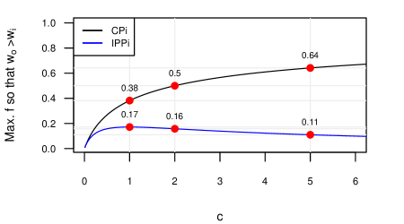
Figure 5: Maximum fraction $f$ of the replication study already completed so that $w_{o}>w_{i}$ in formulas (11) (CPi) and (12) (IPPi).

B.6 Asymptote of IPPi

For $n_{j}\to\infty$, the limiting value of the IPPi is

$$\lim_{n_{j}\to\infty}\text{IPPi} =\Phi\left[\sqrt{\frac{1}{n_{i}/n_{o}+1}}\,t_{o}+\sqrt{\frac{n_{i}/n_{o}}{n_{i}/n_{o}+1}}\,t_{i}\,\right]\,.$$

B.7 Minimum PPi

As the PPi formula in (24) is identical to the fully Bayesian power formula in (19) with $n_{i}=n_{o}$, $n_{j}=n_{r}$ and $\hat{\theta}_{i}=\hat{\theta}_{o}$, the minimum PPi is simply $\Phi\left[\sqrt{t_{i}^{2}-z_{\alpha/2}^{2}}\right]$.

Appendix C Package ReplicationSuccess

Installation

# install the package
install.packages("ReplicationSuccess",
                 repos = "http://R-Forge.R-project.org")
# load the package 
library("ReplicationSuccess")

Data

# load the data
data(SSRP)

Table 4: Main variables of the SSRP dataset.

study	Authors of the original paper
ro	Original effect on correlation scale
ri	Interim effect on correlation scale
rr	Replication effect on correlation scale
fiso	Original effect on Fisher-$z$ scale
fisi	Interim effect on Fisher-$z$ scale
fisr	Replication effect on Fisher-$z$ scale
se_fiso	Standard error of fiso
se_fisi	Standard error of fisi
se_fisr	Standard error of fisr
no	Nominal sample size in original study
ni	Nominal sample size in replication study at interim
nr	Nominal sample size in replication study at the final analysis
po	Two-sided $p$-value from original study
pi	Two-sided $p$-value from interim analysis
pr	Two-sided $p$-value from replication study

Table 4 shows the main variables of the SSRP dataset.

Functions

The two main functions that were used in this paper are powerSignificance and powerSignificanceInterim. The main arguments of these functions are presented in Table 5.

Table 5: Arguments of the powerSignificance and powerSignificanceInterim functions. Arguments only used in powerSignificanceInterim are in grey.

zo	$z$-value from original study
zi	$z$-values from interim analysis
c	Ratio of the replication sample size to the original sample size
f	Fraction of the replication study already completed
designPrior	Design prior
analysisPrior	Analysis prior
alternative	Direction of the alternative
level	Significance level
shrinkage	Shrinkage factor for original effect estimate

Examples

# Variables

# z-value from original study
SSRP$zo = SSRP$fiso/SSRP$se_fiso

# z-value at interim
SSRP$zi = SSRP$fisi/SSRP$se_fisi

# relative sample size from figure 4, 
# where stage 2 is ignored 
# (results at interim are considered 
# final results)
SSRP$c_f3 = (SSRP$ni - 3)/(SSRP$no - 3)

# same values can be found 
# with variance ratio
# SSRP$c_f3 = SSRP$se_fiso^2/SSRP$se_fisi^2

# relative sample size
SSRP$c = (SSRP$nr - 3)/(SSRP$no - 3)

# same values with variance ratio
# SSRP$c = SSRP$se_fiso^2/SSRP$se_fisr^2

# fraction of replication study 
# already completed
SSRP$f = (SSRP$ni - 3)/(SSRP$nr - 3)

# same result 
# with variance ratio
# SSRP$f = SSRP$se_fisr^2/SSRP$se_fisi^2 

# Example : calculation of the predictive power from Fig. 4

powerSignificance(zo = SSRP$zo,
                  c = SSRP$c_f3,
                  designPrior = "predictive",
                  shrinkage = 0.25,
                  alternative = "two.sided",
                  level = 0.05)

# Example: calculation of the informed predictive power 
# at interim (IPPi) from Table 3

# select the studies that were continued 
# after the interim analysis
SSRP_cont <- SSRP[!is.na(SSRP$rr),]

powerSignificanceInterim(zo = SSRP_cont$zo,
                         zi = SSRP_cont$zi,
                         c = SSRP_cont$c,
                         f = SSRP_cont$f,
                         designPrior = "informed predictive",
                         analysisPrior = "flat",
                         alternative = "two.sided",
                         level = 0.05)

References

- Ackerman et al., (2010) Ackerman, J. M., Nocera, C. C., and Bargh, J. A. (2010). Incidental haptic sensations influence social judgments and decisions. Science, 328(5986):1712–1715.
- Anderson and Maxwell, (2017) Anderson, S. F. and Maxwell, S. E. (2017). Addressing the replication crisis: Using original studies to design replication studies with appropriate statistical power. Multivariate Behavioral Research, 52(3):305–324.
- Bauer and König, (2006) Bauer, P. and König, F. (2006). The reassessment of trial perspectives from interim data–a critical view. Statistics in Medicine, 25(1):23–36.
- Begley and Ioannidis, (2015) Begley, C. G. and Ioannidis, J. P. (2015). Reproducibility in science. Circulation Research, 116(1):116–126.
- Button et al., (2013) Button, K. S., Ioannidis, J. P., Mokrysz, C., Nosek, B. A., Flint, J., Robinson, E. S., and Munafò, M. R. (2013). Power failure: why small sample size undermines the reliability of neuroscience. Nature Reviews Neuroscience, 14(5):365.
- Camerer et al., (2016) Camerer, C. F., Dreber, A., Forsell, E., Ho, T.-H., Huber, J., Johannesson, M., Kirchler, M., Almenberg, J., Altmejd, A., Chan, T., Heikensten, E., Holzmeister, F., Imai, T., Isaksson, S., Nave, G., Pfeiffer, T., Razen, M., and Wu, H. (2016). Evaluating replicability of laboratory experiments in economics. Science, 351(6280):1433–1436.
- Camerer et al., (2018) Camerer, C. F., Dreber, A., Holzmeister, F., Ho, T.-H., Huber, J., Johannesson, M., Kirchler, M., Nave, G., Nosek, B. A., Pfeiffer, T., Altmejd, A., Buttrick, N., Chan, T., Chen, Y., Forsell, E., Gampa, A., Heikensten, E., Hummer, L., Imai, T., Isaksson, S., Manfredi, D., Rose, J., Wagenmakers, E.-J., and Wu, H. (2018). Evaluating the replicability of social science experiments in Nature and Science between 2010 and 2015. Nature Human Behaviour, 2(9):637–644.
- Dallow and Fina, (2011) Dallow, N. and Fina, P. (2011). The perils with the misuse of predictive power. Pharmaceutical Statistics, 10(4):311–317.
- DeMets, (2006) DeMets, D. L. (2006). Futility approaches to interim monitoring by data monitoring committees. Clinical Trials, 3(6):522–529.
- Duncan et al., (2012) Duncan, K., Sadanand, A., and Davachi, L. (2012). Memory’s penumbra: Episodic memory decisions induce lingering mnemonic biases. Science, 337(6093):485–487.
- FDA, (1998) FDA (1998). Providing clinical evidence of effectiveness for human drug and biological products. Technical report, US Food and Drug Administration. www.fda.gov/regulatory-information/search-fda-guidance-documents/providing-clinical-evidence-effectiveness-human-drug-and-biological-products.
- Fisher, (1999) Fisher, L. D. (1999). One large, well-designed, multicenter study as an alternative to the usual fda paradigm. Drug Information Journal, 33(1):265–271.
- Gibson, (2020) Gibson, E. W. (2020). The role of p-values in judging the strength of evidence and realistic replication expectations. Statistics in Biopharmaceutical Research, 13(1):6–18.
- Goodman, (1992) Goodman, S. N. (1992). A comment on replication, -values and evidence. Statistics in Medicine, 11(7):875–879.
- Grouin et al., (2007) Grouin, J.-M., Coste, M., Bunouf, P., and Lecoutre, B. (2007). Bayesian sample size determination in non-sequential clinical trials: Statistical aspects and some regulatory considerations. Statistics in Medicine, 26(27):4914–4924.
- Halperin et al., (1982) Halperin, M., Lan, K. G., Ware, J. H., Johnson, N. J., and DeMets, D. L. (1982). An aid to data monitoring in long-term clinical trials. Controlled Clinical Trials, 3(4):311 – 323.
- Held, (2020) Held, L. (2020). A new standard for the analysis and design of replication studies (with discussion). Journal of the Royal Statistical Society: Series A (Statistics in Society), 183(2):431 – 448.
- Herson, (1979) Herson, J. (1979). Predictive probability early termination plans for phase II clinical trials. Biometrics, 35(4):775–783.
- ICH E9 Expert Working Group, (1999) ICH E9 Expert Working Group (1999). Statistical principles for clinical trials: Ich harmonised tripartite guideline. Statistics in Medicine, 18:1905–1942.
- Ioannidis, (2008) Ioannidis, J. P. (2008). Why most discovered true associations are inflated. Epidemiology, 19(5):640–648.
- Jennison and Turnbull, (1999) Jennison, C. and Turnbull, B. W. (1999). Group Sequential Methods with Applications to Clinical Trials. Chapman and Hall/CRC.
- Jiang and Yu, (2016) Jiang, W. and Yu, W. (2016). Power estimation and sample size determination for replication studies of genome-wide association studies. BMC genomics, 17(1):19–32.
- Kieser and Friede, (2003) Kieser, M. and Friede, T. (2003). Simple procedures for blinded sample size adjustment that do not affect the type I error rate. Statistics in Medicine, 22(23):3571–3581.
- Kunzmann et al., (2020) Kunzmann, K., Grayling, M. J., Lee, K. M., Robertson, D. S., Rufibach, K., and Wason, J. M. S. (2020). Conditional power and friends: The why and how of (un)planned, unblinded sample size recalculations in confirmatory trials. https://arxiv.org/abs/2010.06567.
- Lachin, (2005) Lachin, J. M. (2005). A review of methods for futility stopping based on conditional power. Statistics in Medicine, 24(18):2747–2764.
- Lakens, (2014) Lakens, D. (2014). Performing high-powered studies efficiently with sequential analyses. European Journal of Social Psychology, 44(7):701–710.
- Ly et al., (2018) Ly, A., Etz, A., Marsman, M., and Wagenmakers, E.-J. (2018). Replication Bayes factors from evidence updating. Behavior Research Methods, 51(6):2498–2508.
- Matthews, (2006) Matthews, J. N. (2006). Introduction to Randomized Controlled Clinical Trials. Chapman and Hall/CRC.
- O’Hagan and Stevens, (2001) O’Hagan, A. and Stevens, J. W. (2001). Bayesian assessment of sample size for clinical trials of cost-effectiveness. Medical Decision Making, 21(3):219–230. PMID: 11386629.
- O’Hagan et al., (2005) O’Hagan, A., Stevens, J. W., and Campbell, M. J. (2005). Assurance in clinical trial design. Pharmaceutical Statistics, 4(3):187–201.
- Open Science Collaboration, (2015) Open Science Collaboration (2015). Estimating the reproducibility of psychological science. Science, 349(517):aac4716.
- Patil et al., (2016) Patil, P., Peng, R. D., and Leek, J. T. (2016). What should researchers expect when they replicate studies? A statistical view of replicability in psychological science. Perspectives on Psychological Science, 11(4):539–544.
- Pawel and Held, (2020) Pawel, S. and Held, L. (2020). Probabilistic forecasting of replication studies. PLOS ONE. to appear.
- Ramirez and Beilock, (2011) Ramirez, G. and Beilock, S. L. (2011). Writing about testing worries boosts exam performance in the classroom. Science, 331(6014):211–213.
- Rufibach et al., (2016) Rufibach, K., Burger, H. U., and Abt, M. (2016). Bayesian predictive power: choice of prior and some recommendations for its use as probability of success in drug development. Pharmaceutical Statistics, 15(5):438–446.
- Shah et al., (2012) Shah, A. K., Mullainathan, S., and Shafir, E. (2012). Some consequences of having too little. Science, 338(6107):682–685.
- Snapinn et al., (2006) Snapinn, S., Chen, M.-G., Jiang, Q., and Koutsoukos, T. (2006). Assessment of futility in clinical trials. Pharmaceutical Statistics: The Journal of Applied Statistics in the Pharmaceutical Industry, 5(4):273–281.
- Spiegelhalter et al., (2004) Spiegelhalter, D. J., Abrams, K. R., and Myles, J. P. (2004). Bayesian Approaches to Clinical Trials and Health-Care Evaluation. John Wiley & Sons.
- Spiegelhalter and Freedman, (1986) Spiegelhalter, D. J. and Freedman, L. S. (1986). A predictive approach to selecting the size of a clinical trial, based on subjective clinical opinion. Statistics in Medicine, 5(1):1–13.
- Spiegelhalter et al., (1986) Spiegelhalter, D. J., Freedman, L. S., and Blackburn, P. R. (1986). Monitoring clinical trials: conditional or predictive power? Controlled Clinical Trials, 7(1):8–17.
- Wang et al., (2013) Wang, Y., Fu, H., Kulkarni, P., and Kaiser, C. (2013). Evaluating and utilizing probability of study success in clinical development. Clinical Trials, 10(3):407–413.
- Wassmer and Brannath, (2016) Wassmer, G. and Brannath, W. (2016). Group Sequential and Confirmatory Adaptive Designs in Clinical Trials. Springer International Publishing.