Hardness of Identity Testing for Restricted Boltzmann Machines and Potts models

Abstract

We study identity testing for restricted Boltzmann machines (RBMs), and more generally for undirected graphical models. Given sample access to the Gibbs distribution corresponding to an unknown or hidden model $M^{*}$ and given an explicit model $M$, can we distinguish if either $M=M^{*}$ or if they are (statistically) far apart? Daskalakis et al. (2018) presented a polynomial-time algorithm for identity testing for the ferromagnetic (attractive) Ising model. In contrast, for the antiferromagnetic (repulsive) Ising model, Bezáková et al. (2019) proved that unless $\textsc{RP}=\textsc{NP}$ there is no identity testing algorithm when $\beta d=\omega(\log{n})$, where $d$ is the maximum degree of the visible graph and $\beta$ is the largest edge weight (in absolute value).

We prove analogous hardness results for RBMs (i.e., mixed Ising models on bipartite graphs), even when there are no latent variables or an external field. Specifically, we show that if $\textsc{RP}\neq\textsc{NP}$, then when $\beta d=\omega(\log{n})$ there is no polynomial-time algorithm for identity testing for RBMs; when $\beta d=O(\log{n})$ there is an efficient identity testing algorithm that utilizes the structure learning algorithm of Klivans and Meka (2017). In addition, we prove similar lower bounds for purely ferromagnetic RBMs with inconsistent external fields, and for the ferromagnetic Potts model. Previous hardness results for identity testing of Bezáková et al. (2019) utilized the hardness of finding the maximum cuts, which corresponds to the ground states of the antiferromagnetic Ising model. Since RBMs are on bipartite graphs such an approach is not feasible. We instead introduce a novel methodology to reduce from the corresponding approximate counting problem and utilize the phase transition that is exhibited by RBMs and the mean-field Potts model. We believe that our method is general, and that it can be used to establish the hardness of identity testing for other spin systems.

1 Introduction

For graphical models, there are several fundamental computational tasks which are essential for utilizing these models. These computational problems can be broadly labeled as follows: sampling, counting, structure learning, and testing. Our big picture aim is to understand the relationship between these problems. The specific focus in this paper is on the computational complexity of the identity testing problem for undirected graphical models and its connections to the hardness of the counting problem.

Identity testing is a basic question in statistics for testing whether a given model fits a dataset. Roughly speaking, given data $\mathcal{D}$ sampled from the posterior or likelihood distribution of an unknown/hidden model $M^{*}$ and given an explicit model $M$, can we distinguish whether $M=M^{*}$?

We study identity testing in the context of undirected graphical models [39], which correspond to (pairwise) Markov random fields in probability theory and computer vision [22] and to spin systems in statistical physics [23]. We focus attention on examples of graphical models of particular interest: the Ising model, the Potts model, and Restricted Boltzmann Machines. The Ising model is the simplest example of an undirected graphical model, and, in fact, it is one of the most well-studied models in statistical physics where it is used to study phase transitions. The Potts model is the generalization of the Ising model from a two state system to an integer $q\geq 3$ state system. It is also well-studied in statistical physics as the nature of the phase transition changes as $q$ increases [14, 15].

Restricted Boltzmann Machines (RBMs) are a simple class of undirected graphical models corresponding to the Ising model on bipartite graphs. Originally introduced by Smolensky in 1986 [47], they have played an important role in the history of computational learning theory. They have two layers of variables: one layer corresponding to the observed variables and another layer corresponding to the hidden/latent variables, and no intralayer connections so that the underlying graph is bipartite. Learning was shown to be practical in these restricted models [31, 32] and henceforth played a seminal role in the development of deep learning [42, 40, 43, 33].

We define first the Potts model, as both the Ising model and RBMs may be viewed as special cases of this model. The Potts model is specified by a graph $G=(V,E)$, a set of vertex labels or spins $[q]=\{1,\dots,q\}$, a set of edge weights defined by $\beta:E\rightarrow\mathbb{R}$ and a set of vertex weights $h:V\times[q]\rightarrow\mathbb{R}$. Configurations of the Potts model are the collection of vertex labelings $\Omega=\{1,\dots,q\}^{V}$. The Gibbs distribution associated with the Potts model is a distribution over all configurations $\sigma\in\Omega$ such that:

$$\mu(\sigma)=\mu_{G,\beta,h}(\sigma):=\frac{1}{Z}\exp\left(\sum_{\{u,v\}\in E}\beta(\{u,v\})\mathbbm{1}(\sigma(u)=\sigma(v))+\sum_{v\in V}h(v,\sigma(v))\right),$$

where $Z=Z_{G,\beta,h}$ is the normalizing factor or partition function given by:

$$Z:=\sum_{\sigma\in\Omega}\exp\left(\sum_{\{u,v\}\in E}\beta(\{u,v\})\mathbbm{1}(\sigma(u)=\sigma(v))+\sum_{v\in V}h(v,\sigma(v))\right).$$

When $\beta(e)>0$ for every $e\in E$, the model is called ferromagnetic and neighboring vertices prefer to align to the same spin. Conversely, when $\beta(e)<0$ for every $e\in E$ the model is called antiferromagnetic. Models where $\beta$ is allowed to be both positive or negative for distinct edges are called mixed models.

The Ising model corresponds to the special case where there are only two spins; i.e., $q=2$. RBMs are mixed Ising models restricted to bipartite graphs; that is, $G$ is bipartite with bipartition $V=L\cup R$. Since the focus in this paper is on lower bounds, we often consider the case of no external field ($h=0$) in order to obtain stronger hardness results.

Given a model specification, that is, a graph $G=(V,E)$, an edge weight function $\beta$ and an external field $h$, the goal in the sampling problem is to generate samples from the Gibbs distribution $\mu=\mu_{G,\beta,h}$ (or from a distribution close to $\mu$ in total variation distance). The corresponding counting problem is to compute the partition function $Z=Z_{G,\beta,h}$. The (exact) counting problem is #P-hard [51] even for restricted classes of graphs [27, 50], and hence the focus on the approximate counting problem of obtaining an $\mathsf{FPRAS}$ (fully-polynomial randomized approximation scheme) for $Z$. For a general class of models, the approximate counting and the approximate sampling problems are equivalent, i.e., there are polynomial-time reductions between them [35, 48, 37]. A seminal result of Jerrum and Sinclair [34] (see also [41, 10, 29]) presented an $\mathsf{FPRAS}$ for the partition function of the ferromagnetic Ising model.

Another two fundamental problems for undirected graphical models are structure learning and identity testing. The structure learning problem is as follows: given oracle access to samples from the Gibbs distribution $\mu_{M^{*}}$ for an unknown (i.e., “hidden”) model $M^{*}=(G^{*},\beta^{*},h^{*})$, can we learn $G^{*}$ (i.e., the structure of the model) in polynomial-time with probability at least $2/3$? In the case of no latent variables (so the samples from the Gibbs distribution reveal the label of all vertices $V$ of $G$) recent work of Klivans and Meka [36] (see also [5, 53, 30, 52, 54]) learns $n$-vertex graphs with $O(\log{n})\times\exp(O(\beta d))$ samples and $O(n^{2}\log{n})\times\exp(O(\beta d))$ time where $d$ is the maximum degree of $G$ and $\beta:=\max_{e\in E}|\beta(e)|$ is the maximum edge weight in absolute value; this bound has nearly-optimal sample complexity from an information-theory perspective [44].

For RBMs with latent variables (thus samples only reveal the labels for vertices on one side $R$), structure learning can be done in time $O(n^{d_{L}+1})$ where $d_{L}$ is the maximum degree of the latent variables. Recent work of Bresler, Koehler and Moitra [6] proves that there is no algorithm with running time $n^{o(d_{L})}$ assuming $k$-sparse noisy parity on $n$ bits is hard to learn in time $n^{o(k)}$; they also show that for the special case of ferromagnetic RBMs with hidden variables there is a structure learning algorithm with $O(\log{n})\times\exp(O(\beta d^{2}))$ sample complexity and $O(n^{2}\log{n})\times\exp(O(\beta d^{2}))$ running time.

In the identity testing problem we are given oracle access to samples from the Gibbs distribution $\mu_{M^{*}}$ for an unknown model $M^{*}=(G^{*},\beta^{*},h^{*})$ (as in structure learning) and we are also given an explicit model $M=(G,\beta,h)$. Our goal is to determine, with probability $\geq 2/3$, if either $M=M^{*}$ or if the models are $(1-\varepsilon)$-far apart; specifically, if the total variation distance between their Gibbs distributions is at least $1-\varepsilon$ for a given $\varepsilon>0$. (We note that previous works assumed separation $\geq\varepsilon$ in the later case, whereas we prove hardness even when we assume separation $\geq 1-\varepsilon$.)

It is known that identity testing cannot be solved in polynomial time for general graphical models in the presence of hidden variables unless $\textsc{RP}=\textsc{NP}$ [3] . In this paper we assume there are no hidden variables and hence the samples from $\mu_{M^{*}}$ reveal the label of every vertex in the graph $G$; this setting is more interesting for hardness results. We explore a more refined picture of hardness of identity testing vs. polynomial-time algorithms.

It is known that identity testing can be reduced to sampling [13] or structure learning [1]: given an efficient algorithm for the associated sampling problem or an efficient algorithm for structure learning, then one can efficiently solve the identity testing problem. Hence, identity testing is (computationally) easier than sampling and structure learning. (To be precise, one needs to solve both the structure learning and the parameter estimation problems to solve identity testing; the algorithm of Klivans and Meka [36] does in fact provide this.) This raises the question of whether identity testing can be efficiently solved in cases where sampling and structure learning are known to be hard. We prove (for the models studied here) that when sampling and structure learning are hard, then identity testing is also hard.

1.1 Our results

The $\varepsilon$-identity testing problem for the Ising and Potts models is formally defined as follows. For positive integers $n$ and $d$, and positive real numbers $\beta$ and $h$, let $\mathcal{M}_{\textsc{RBM}}(n,d,\beta,h)$ denote the family of RBMs on $n$-vertex bipartite graphs $G=(V,E)$ of maximum degree at most $d$, where the absolute value of all edge interactions is at most $\beta$ and the field $|h(v,i)|\leq h$ for all $v\in V$ and $i\in[q]$; see Definition 2.1. We define $\mathcal{M}_{\textsc{Potts}}(n,d,\beta,h)$ analogously for the family of Potts models, without the restriction of $G$ being bipartite.

Given an RBM $M\in\mathcal{M}_{\textsc{RBM}}(n,d,\beta,h)$, and sample access to a distribution $\mu_{M^{*}}$ for an unknown RBM $M^{*}\in\mathcal{M}_{\textsc{RBM}}(n,d,\beta,h)$, distinguish with probability at least $3/4$ between the cases: 1. $\mu_{M}=\mu_{M^{*}}$;            2. ${\|\mu_{M}-\mu_{M^{*}}\|}_{\textsc{tv}}\geq 1-\varepsilon$.

The choice of $3/4$ for the probability of success is arbitrary, and it can be replaced by any constant in the interval $(\frac{1}{2},1)$ at the expense of a constant factor in the running time of the algorithm. The $\varepsilon$-identity testing problem for the Potts model is defined in the same manner, but assuming that both $M$ and $M^{*}$ belong to $\mathcal{M}_{\textsc{potts}}(n,d,\beta,h)$ instead.

Our first result concerns the identity testing problem on $\mathcal{M}_{\textsc{RBM}}(n,d,\beta,0)$; that is, (mixed) RBMs without external fields: $h(v,i)=0$ for all $v\in V$, $i\in[q]$. We show that for RBMs the approach utilizing structure learning is essentially best possible. In particular we prove that when $\beta d=\omega(\log{n})$ there is no poly-time identity testing algorithm, unless $\textsc{RP}=\textsc{NP}$. Note that when $\beta d=O(\log{n})$, the algorithm of Klivans and Meka [36] for structure learning and parameter estimation provides an identity testing algorithm with $\mathrm{poly}(n)$ sample complexity and running time.

Theorem 1.1.

Suppose $n$, $d$ are positive integers such that $3\leq d\leq n^{\theta}$ for constant $\theta\in(0,1)$ and let $\varepsilon\in(0,1)$. If $\textsc{RP}\neq\textsc{NP}$, then for all real $\beta>0$ satisfying $\beta d=\omega(\log n)$ there is no polynomial running time algorithm to solve the $\varepsilon$-identity testing problem for the class $\mathcal{M}_{\textsc{RBM}}(n,d,\beta,0)$ of mixed RBMs without external fields.

In contrast to the above result, Daskalakis, Dikkala and Kamath [13] provided a poly-time identity testing algorithm for all ferromagnetic Ising model with consistent fields (the external field is consistent if it only favors the same unique spin at every vertex; otherwise it is called inconsistent; see Definition 4.1). Their algorithm crucially utilizes the known poly-time sampling methods for the ferromagnetic Ising model [34, 41, 10, 29]. On the hardness side, super-polynomial lower bounds were recently established for identity testing for the antiferromagnetic Ising model on general (not necessarily bipartite) graphs when $\beta d=\omega(\log{n})$ [1]. This previous result utilizes the hardness of the maximum cut problem, since maximum cuts correspond to the “ground states” (maximum likelihood configurations) of the antiferromagnetic model; this is not the case for RBMs, and new insights are required (see Section 1.2 for a more detailed discussion). In particular we show a new approach to reduce from the counting problem.

Ferromagnetic and antiferromagnetic RBMs are equivalent models; that is, there is a one-to-one correspondence between configurations with the same weight. Hence, the results in [13] solve the identity testing problem for both ferromagnetic and antiferromagnetic RBMs with no latent variables, even in the presence of a consistent external field. Moreover, Klivans and Meka’s algorithm from [36] together with the hardness results of Theorem 1.1 provides a fairly complete picture of the computational complexity of identity testing for (mixed) RBMs with no external field ($h=0$).

Our next result concerns the hardness of identity testing for purely ferromagnetic RBMs with an inconsistent magnetic field; that is, a field that favors one spin for some of the vertices and the other spin for the rest; see Definition 4.1. For this we utilize the complexity of #BIS, which is the problem of counting the independent sets in a bipartite graph. #BIS is believed not to have an $\mathsf{FPRAS}$, and it has achieved considerable interest in approximate counting as a tool for proving relative complexity hardness [16, 26, 17, 7, 9, 8, 18]. Let $\mathcal{M}^{+}_{\textsc{RBM}}(n,d,\beta,h)$ be set of all ferromagnetic RBMs in $\mathcal{M}_{\textsc{RBM}}(n,d,\beta,h)$.

Theorem 1.2.

Suppose $n$, $d$ are positive integers such that $3\leq d\leq n^{\theta}$ for constant $\theta\in(0,1)$ and let $\varepsilon\in(0,1)$. If #BIS does not admit an $\mathsf{FPRAS}$, there exists $h=O(1)$ such that when $\beta d=\omega(\log n)$ there is no polynomial running time algorithm that solves the $\varepsilon$-identity testing problem for the class $\mathcal{M}^{+}_{\textsc{RBM}}(n,d,\beta,h)$ of ferrromagnetic RBMs with inconsistent external fields.

Given the efficient identity testing algorithm for ferromagnetic Ising models [13, 34], we may ask whether there are other (ferromagnetic) models that allow efficient testing algorithms. A prime candidate is the ferromagnetic Potts model. Both the ferromagnetic Ising and Potts models have a rich structure; for instance, their random-cluster representation [28] enables sophisticated (and widely-used) sampling algorithms such as the Swendsen-Wang algorithm [49]. However, while there are efficient samplers for the ferromagnetic Ising model for all graphs $G$ and all edge interactions $\beta$ [34, 10, 29], the case of the ferromagnetic Potts model (i.e., $q>2$ spins) looks less promising. In fact, it is unlikely that there is an efficient sampling/counting algorithm for general ferromagnetic Potts models since this is a known #BIS-hard problem [26, 19]; this is due to a phenomena called phase co-existence, which we will also exploit; see Section 2.2.1. Given the weaker hardness of sampling and approximate counting for the ferromagnetic Potts model, the hardness of the identity problem was less clear.

We prove that identity testing for the ferromagnetic Potts model is in fact hard in the same regime of parameters where sampling and structure learning are known to be hard. Specifically, we observe that the structure learning algorithm from [36] applies to the Potts model, and hence implies a testing algorithm when $\beta d=O(\log{n})$; we establish lower bounds when $\beta d=\omega(\log{n})$ that hold even for the simpler case of models with no external field.

Theorem 1.3.

Suppose $n$, $d$, $q\geq 3$ are positive integers such that $3\leq d\leq n^{\theta}$ for constant $\theta\in(0,1)$ and let $\varepsilon\in(0,1)$. If #BIS does not admit an $\mathsf{FPRAS}$, then there is no polynomial running time algorithm that solves the $\varepsilon$-identity testing problem for the class $\mathcal{M}^{+}_{\textsc{Potts}}(n,d,\beta,0)$ of ferromagnetic $q$-state Potts models without an external field. Moreover, our lower bound applies restricted to the class of ferromagnetic Potts models on bipartite graphs in $\mathcal{M}^{+}_{\textsc{Potts}}(n,d,\beta,0)$.

1.2 Our techniques

Our proof is a general approach that allows us to obtain hardness results for several models of interest. Specifically, we devise a novel methodology to reduce the problem of approximate counting (i.e., approximating partition functions) to identity testing. For this we consider a decision version of approximate counting and prove that this variant is as hard as the standard approximation problem; this first step of our reduction applies to many other models of interest (see Theorem 2.4 and Section 6).

In the second step of our reduction, given a hard counting instance, we use insights about the phase transition of the models to construct a testing instance whose output allows us to solve the decision version of approximate counting. The actual reduction is generic (see Theorem 2.11), but the insights about each model are needed to build a suitable testing instance; this construction is the only part of our proof that is model specific, whereas every other step in the proof applies to more general spin systems. Our approach is nicely illustrated in the context of the ferromagnetic Potts model; that is, in the proof of Theorem 1.3 in Section 2. There, we utilize the phase transition phenomenon in the associated mean-field Potts model which corresponds to the complete graph. In particular, there is a phase co-existence corresponding to a first-order phase transition which we utilize to approximate the partition function of the input graph; see Section 2.

In the third and final step of the reduction, we reduce the maximum degree of the graph in the testing instance by using random bipartite graphs as gadgets, as has been done in seminal hardness results for approximate counting [45, 46], and more recently in [1] for the hardness of testing for the antiferromagnetic Ising model. This step is also generic and applies to a large class of models; see Section 5 and specifically Theorem 5.2. One interesting implication of our approach is that our gadget and reduction yields always bipartite graphs, and hence we immediately get hardness results for bipartite graphs for all of the models studied in this paper.

We pause to briefly contrast the above proof approach with that in [1], where it was established hardness of identity testing for the antiferromagnetic Ising model. As mentioned earlier, in the antiferromagnetic Ising model, the configurations with the highest weight or likelihood (i.e., the ground states) correspond to the maximum cuts of the original graph. Hence, it is natural to prove hardness of identity testing for the antiferromagnetic Ising model using a reduction from the maximum cut problem. The ground states of ferromagnetic systems, on the other hand, correspond to the monochromatic configurations, so there is no hard optimization problem in the background to utilize in the reduction. (The similar obstacle for RBMs is that the maximum cut problem is trivial in bipartite graphs, so we cannot hope to use it to prove hardness.) We use the hardness of approximating the partition function instead, and consequently our reduction is of a completely different flavor (than [1]); we utilize the unique nature of the phase transition in these models in an essential way.

To reduce the degree of the graphs in our construction we do utilize insights and certain technical lemmas from [1]. Specifically, those concerning the expansion of random near-regular bipartite graphs. We note that the models we consider on these random graphs are different than those in [1]; in particular, we consider mixed models and allowed external fields, whereas in  [1] these gadgets are purely antiferromagnetic and there is no external field.

We present our proof approach in the context of the ferromagnetic Potts model first, specifically in Section 2 we prove Theorem 1.3. The proofs for RBMs, namely Theorems 1.1 and 1.2 which follow the same approach, are provided in Sections 3 and 4, respectively.

2 Testing ferromagnetic Potts models

In this section we prove Theorem 1.3, our lower bound for identity testing for the ferromagnetic Potts model. To prove this theorem, we introduce a new methodology to reduce approximate counting (i.e., the problem of finding an $\mathsf{FPRAS}$ for the partition function of a model), to identity testing. We later use this framework to establish our lower bounds for identity testing for RBMs (i.e., Theorems 1.1 and 1.2); we believe our methods could be used to establish the hardness of identity testing for other spin systems.

We introduce some useful notation next. Recall that in the introduction we define the families of models $\mathcal{M}_{\textsc{RBM}}$, $\mathcal{M}^{+}_{\textsc{RBM}}$, $\mathcal{M}_{\textsc{Potts}}$ and $\mathcal{M}^{+}_{\textsc{Potts}}$. We formalize and extend this notation as follows.

Definition 2.1.

For integers $n,d\geq 3$ and $\beta,h\in\mathbb{R}$, let $\mathcal{M}_{\textsc{Potts}}(n,d,\beta,h,q)$ denote the family of $q$-state Potts models on $n$-vertex graphs $G=(V_{G},E_{G})$ of maximum degree at most $d$ with edge interactions and external field given by $\beta_{G}:E_{G}\rightarrow\mathbb{R}$ and $h_{G}:V_{G}\times[q]\rightarrow\mathbb{R}$, respectively, such that:

1. for every edge $\{u,v\}\in E_{G}$, $|\beta_{G}(\{u,v\})|\leq\beta$; and

2. for every vertex $v\in V_{G}$ and spin $i\in[q]$, $|h_{G}(v,i)|\leq h$.

Remark 2.2.

We omit $q$ from the notation above as it is usually clear from context. For the special case of $q=2$, i.e., the Ising model, we use $\mathcal{M}_{\textsc{Ising}}$; when $q=2$ and the underlying graph is bipartite we use $\mathcal{M}_{\textsc{RBM}}$. In addition, we add “$+$” or “$-$” as a superscript to the notation to denote the corresponding ferromagnetic or antiferromagnetic subfamilies; e.g., $\mathcal{M}^{+}_{\textsc{Potts}}(n,d,\beta,h)$ denotes the subset of ferromagnetic Potts models in $\mathcal{M}_{\textsc{Potts}}(n,d,\beta,h)$. Finally, we add a circumflex, e.g., $\mathcal{\hat{M}}^{+}_{\textsc{Potts}}(n,d,\beta,h)$, for the subfamily of models where every edge weight is exactly equal to $\beta$.

2.1 Step 1: Decision version of approximate counting

Our starting point is always a known hard approximate counting instance. For the ferromagnetic Potts model, we consider the problem of approximating its partition function on a graph $G$. As mentioned in the introduction, this problem is known to be #BIS-hard, even under the additional assumptions that all edges have the same interaction parameter $0<\beta_{G}=\Theta(1)$ and that there is no external field (i.e., $h=0$) [26, 19]. Our goal is to design an $\mathsf{FPRAS}$ for the partition function $Z_{G,\beta_{G}}:=Z_{G,\beta_{G},0}$ using a polynomial-time algorithm for identity testing, thus establishing the #BIS-hardness of this problem.

Our first step is to reduce the problem of approximating $Z_{G,\beta_{G}}$ to a natural decision variant of the problem. This decision version will be more naturally solved by the testing algorithm and is more generally defined as follows:

Definition 2.3 (Decision $r$-approximate counting).

Given a Potts model ($G$,$\beta_{G}$,$h_{G}$), an approximation ratio $r>1$ and an input $\hat{Z}\in\mathbb{R}$, distinguish with probability at least $5/8$ between the following two cases: $$\text{(i)}~{}Z_{G,\beta_{G},h_{G}}\leq\frac{1}{r}\hat{Z}\quad\quad\text{(ii)}~{}Z_{G,\beta_{G},h_{G}}\geq r\hat{Z}$$

We show that the decision version of approximate counting is as hard as the standard problem of approximating $Z_{G,\beta_{G},h_{G}}$.

Theorem 2.4.

Let $n,d\geq 1$ be integers and let $\beta,h\geq 0$ be real numbers. Suppose that there is no $\mathsf{FPRAS}$ for the counting problem for a family of Potts models $\mathcal{M}$, where

$$\mathcal{M}\in\{\mathcal{\hat{M}}^{+}_{\textsc{Potts}}(n,d,\beta,h),\mathcal{\hat{M}}^{-}_{\textsc{Ising}}(n,d,\beta,h),\mathcal{\hat{M}}^{+}_{\textsc{Ising}}(n,d,{\beta},{h})\}.$$

Then, for any $c>0$ there is no polynomial-time algorithm for the decision version of $n^{c}$-approximate counting for $\mathcal{M}$.

Our proof of this theorem is provided in Section 6.

2.2 Step 2: Testing instance construction

We first construct a hard instance for the identity testing problem for the ferromagnetic Potts model on general graphs, with no restriction on the maximum degree and with a constant upper bound on the edge interactions. We prove first that identity testing is #BIS-hard in this setting.

Theorem 2.5.

Consider a ferromagnetic Potts model with no external field ($h=0$) where the interaction on every edge is ferromagnetic and bounded from above by a constant $\beta_{0}>0$. Then, there is no polynomial-time identity testing algorithm for the model unless there is an $\mathsf{FPRAS}$ for #BIS.

To establish this theorem, we construct an identity testing instance that allows us to solve the decision variant of approximate counting (see Definition 2.3). We note that this theorem does not immediately imply Theorem 1.3 from the introduction because we allow the degree to be unbounded; specifically, Theorem 2.5 establishes hardness for $\mathcal{M}^{+}_{\textsc{Potts}}(n,n,\beta,0)$. The next step of the proof uses this result and a degree-reducing gadget to establish Theorem 1.3 (see Section 2.3). Our main gadget in the proof of Theorem 2.5 will be a complete graph $H$ on $m$ vertices; this is known as the mean-field case in statistical physics.

2.2.1 The ferromagnetic mean-field $q$-state Potts model

Let $H=K_{m}$ be a complete graph on $m$ vertices and let $\beta_{H}$ be the interaction strength on the edges of $H$. By symmetry, the $q$-state Potts configurations on a complete graph can be described by their “signature”—by “signature” we mean the vector $(\sigma_{1},\dots,\sigma_{q})\in\mathbb{Z}^{q}$ where $\sigma_{i}\geq 0$ is the number of vertices that have spin $i$; note that $\sum_{i=1}^{q}\sigma_{i}=m$.

In the complete graph, the ferromagnetic Potts model is known to undergo an “order-disorder” phase transition. Specifically, there exists a critical value $\beta_{H}=\mathfrak{B}_{o}/m$ such that when $\beta_{H}<\mathfrak{B}_{o}/m$, long-range correlations do not exist; the system is then said to be in a “disordered” state as the typical configurations have signature $\approx(m/q,\dots,m/q)$ where each spin has roughly the same density (up to lower order terms). In contrast, when $\beta_{H}>\mathfrak{B}_{o}/m$, typical configurations have a dominant spin and the remaining spins are uniformly distributed. These configurations are thus referred to as “majority” configurations. More precisely there exists a constant $\alpha=\alpha(\beta_{H})>1/q$ and, with high probability, configurations from the Gibbs distribution have signature $\approx\left(\alpha m,\frac{(1-\alpha)m}{q-1},\dots,\frac{(1-\alpha)m}{q-1}\right)$ up to permutations and lower order terms.

When $q\geq 3$, the phase transition is known to be of first-order, which means that at the critical point $\beta_{H}=\mathfrak{B}_{o}/m$ both disordered and majority configurations occur with constant probability. This phenomena is referred to as phase co-existence, and it is known (or conjectured) to be present in a variety of graphs, being the root reason for the hardness of sampling and counting for the ferromagnetic Potts model. In contrast, in the Ising model (i.e., when $q=2$), there is a second-order phase transition and the majority density $\alpha(\mathfrak{B}_{o})$ is $1/q$ at the critical point; hence these two phases – disordered and majority – coincide at this point.

We now formalize the notion of the majority phase $M$, the disordered phase $D$, and the remaining configurations $S$ with their corresponding partition functions $Z_{H}^{\mathrm{M}}$, $Z^{\mathrm{D}}_{H}$, and $Z_{H}^{\SS}$. The majority phase is defined with respect to a fixed constant $\hat{\alpha}=\hat{\alpha}(\mathfrak{B}_{o})$ which is the density of the dominant color at the phase coexistence point $\mathfrak{B}_{o}/m$. Let $\Omega_{H}$ denote the set of Potts configurations on $H$ and for $\sigma\in\Omega_{H}$, let $(\sigma_{1},\dots,\sigma_{q})\in\mathbb{Z}^{q}$ denote its signature. Consider the following sets:

$$M:=\Bigg{\{}\sigma\in\Omega_{H}\,\big{|}\,~{}\exists j\in[q]:~{}|\sigma_{j}-\hat{\alpha}m|\leq m^{3/4}\mbox{ and }\left|\sigma_{i}-\frac{1-\hat{\alpha}}{q-1}m\right|\leq m^{3/4}\ \mbox{for}\ i\in[q]\setminus\{j\}\Bigg{\}},$$

$$D:=\Bigg{\{}\sigma\in\Omega_{H}\,\big{|}\,~{}\forall i\in[q]:~{}|\sigma_{i}-m/q|\leq m^{3/4}\Bigg{\}},$$

and $S:=\Omega_{H}\setminus(M\cup D).$

For a configuration $\sigma$ on the complete graph $H=(E_{H},V_{H})$, let

$$w_{H}^{\sigma}(\beta_{H})=\exp\left(\sum_{\{u,v\}\in E(H)}\beta_{H}\mathbbm{1}(\sigma(u)=\sigma(v))\right)$$

denote the weight of $\sigma$ in the mean-field model $(H,\beta_{H})$. Consider the contributions of each type of configuration to the partition function. That is,

$$Z_{H}^{\mathrm{M}}(\beta_{H}):=\sum_{\sigma\in M}w_{H}^{\sigma}(\beta_{H}),\quad\quad Z_{H}^{\mathrm{D}}(\beta_{H}):=\sum_{\sigma\in D}w_{H}^{\sigma}(\beta_{H}),\quad\quad Z_{H}^{\SS}(\beta_{H}):=\sum_{\sigma\in S}w_{H}^{\sigma}(\beta_{H}).$$

Hence, the partition function of $(H,\beta_{H})$ is given by $Z_{H}(\beta_{H})=Z_{H}^{\mathrm{M}}(\beta_{H})+Z_{H}^{\mathrm{D}}(\beta_{H})+Z_{H}^{\SS}(\beta_{H})$. We note that in our reduction later, we will choose a specific $\beta_{H}>0$ depending on the instance of the approximate counting problem and the parameters of the identity testing algorithm; hence, to emphasize the effect of $\beta_{H}$, we parameterize $Z_{H}^{\mathrm{M}}$ (and other functions in this section) in terms of $\beta_{H}$.

The following two lemmas detail the relevant behavior of the mean-field Potts model at and around the critical point $\mathfrak{B}_{o}/m$. We note that as a consequence of the first-order phase transition, there is a critical window around $\mathfrak{B}_{o}/m$ where the non-dominant phase (i.e., disorder or majority) is still much more likely than any other type configurations; this phenomena is known as metastability and will also be crucial for us.

First we establish that in the critical window around $\mathfrak{B}_{o}/m$ the majority $M$ and disordered $D$ configurations are exponentially more likely than the remaining configurations $S$. Several variants of this result have been proved in some fashion before, e.g., [4, 38, 26, 12, 24, 20, 2]; however, the precise bound we require in our proofs does not seem to be available in the literature.

Lemma 2.6.

There exists constants $c,c^{\prime}>0$ such that for any $\beta_{H}$ satisfying $|\beta_{H}-\mathfrak{B}_{o}/m|\leq c^{\prime}m^{-3/2}$ we have

$$Z_{H}^{\SS}(\beta_{H})\leq\min\{Z_{H}^{\mathrm{M}}(\beta_{H}),Z_{H}^{\mathrm{D}}(\beta_{H})\}\exp(-c\sqrt{m}).$$

In addition, we show that we can find in $\mathrm{poly}(m)$ time a value for the parameter $\beta_{H}$ in the critical window to achieve a specified ratio $R$ of the majority partition function $Z^{\mathrm{M}}_{H}(\beta_{H})$ to the disordered partition function $Z^{\mathrm{D}}_{H}(\beta_{H})$.

Lemma 2.7.

There exist constants $c,c^{\prime}>0$ such that for any $R\in[{e}^{-c\sqrt{m}},{e}^{c\sqrt{m}}]$ and any constant $\delta\in(0,1)$, we can efficiently find $\beta_{H}>0$ in $\mathrm{poly}(m)$ time such that $|\beta_{H}-\mathfrak{B}_{o}/m|\leq c^{\prime}m^{-3/2}$ and

$$(1-\delta)R\leq\frac{Z_{H}^{\mathrm{M}}(\beta_{H})}{Z_{H}^{\mathrm{D}}(\beta_{H})}\leq R.$$ (1)

The proof of these two lemmas is provided in Appendix A.

2.2.2 Identity testing reduction

Visible Model Construction.  Let $(G,\beta_{G})$ be the instance of the ferromagnetic Potts model with no external field (i.e., $h=0$) for which we are trying to approximate the partition function $Z_{G,\beta_{G}}$; we shall assume $G=(V_{G},E_{G})$ is an $N$-vertex graph and that every edge has interaction strength $0<\beta_{G}=\Theta(1)$. Let $H=(V_{H},E_{H})$ be a complete graph on $m=N^{10}$ vertices. The graph $F=(V_{F},E_{F})$ is the result of connecting the vertices of $H$ and $G$ with a complete bipartite graph $K_{m,N}$ with edges $E_{m,N}$; that is, $V_{F}=V_{G}\cup V_{H}$ and $E_{F}=E_{H}\cup E_{G}\cup E_{m,N}$. We consider the Potts model on the graph $F$ with edge interactions $\beta_{F}:E_{F}\rightarrow\mathbb{R}$ given by:

$$\beta_{F}(e)=\left.\begin{cases}\beta_{H}&\text{if }e\in E_{H}\\ \beta_{G}&\text{if }e\in E_{G}\\ \beta&\text{if }e\in E_{m,N},\end{cases}\right.$$

where $\beta_{H},\beta>0$ will be chosen later. We use $n:=N+m$ for the number of vertices of $F$, and, with a slight abuse of notation, we use $F$ for the Potts model $(F,\beta_{F})$ which will play the role of the visible model in our reduction; $\mu_{F}$ denotes the corresponding Gibbs distribution.

We study first the properties of “typical” configurations on $G$ conditional on a configuration $\sigma$ on the complete graph $H$. For this, we introduce some additional notation. Let $\Omega_{F}$, $\Omega_{H}$ and $\Omega_{G}$ be the set of Potts configuration on the graph $F$, $H$ and $G$ respectively; note that $\Omega_{F}=\Omega_{H}\times\Omega_{G}$. For $\sigma\in\Omega_{H}$, define

$$Z_{F}^{\sigma}(\beta_{H}):=\sum_{\eta\in\Omega_{F}:\eta(V_{H})=\sigma}{w_{F}^{\eta}(\beta_{H})}$$

where the weight $w_{F}^{\eta}(\beta_{H})$ of configuration $\eta$ is given by

$$w_{F}^{\eta}(\beta_{H})=\exp\left(\sum_{\{u,v\}\in E_{F}}\beta_{F}(\{u,v\})\mathbbm{1}(\eta(u)=\eta(v))\right);$$

that is, $Z_{F}^{\sigma}(\beta_{H})$ is the total contribution to the partition $Z_{F}(\beta_{H})$ of $F$ of the configurations that agree with $\sigma$ on $H$.

If we fix a configuration $\sigma$ on $H$ and look at the configuration on $G$ (under the Gibbs distribution on $F$ conditional on $\sigma$) then $\sigma$ will act as an external field on the vertices of $G$. We show that if $\sigma$ is in the majority phase (i.e., in the set $M$), then the configuration on $G$ will be monochromatic with high probability as these configurations will maximize the number of monochromatic edges between $G$ and $H$. In contrast, when $\sigma$ is in the disordered phase (i.e., in $D$), then every configuration on $G$ will have (roughly) the same number of monochromatic edges between $G$ and $H$; hence, the partition function $Z_{F}^{\sigma}(\beta_{H})$ in this case will be proportional to $Z_{G,\beta_{G}}$.

To formalize this, we split the partition function of $F$ into three parts depending on the signature on the complete graph $H$. Let

$$Z_{F}^{\mathrm{M}}(\beta_{H})=\sum_{\sigma\in M}Z^{\sigma}_{F}(\beta_{H}),\ \ Z_{F}^{\mathrm{D}}(\beta_{H})=\sum_{\sigma\in D}Z^{\sigma}_{F}(\beta_{H}),\ \mbox{ and }Z_{F}^{\SS}(\beta_{H})=\sum_{\sigma\in S}Z^{\sigma}_{F}(\beta_{H});$$

then, $Z_{F}(\beta_{H})=Z_{F}^{\mathrm{M}}(\beta_{H})+Z_{F}^{\mathrm{D}}(\beta_{H})+Z_{F}^{\SS}(\beta_{H}).$

The following lemma details the above description of the properties of configurations on the original instance $G$ conditional on the configuration on the complete graph $H$.

Lemma 2.8.

For any constants $\delta\in(0,1)$ and $c>0$, and any $\beta_{H}$ such that $|\beta_{H}-\mathfrak{B}_{o}/m|\leq cm^{-3/2}$, there exists constants $c_{1},c_{2}>0$ such that for any $\beta\in\left[\frac{c_{1}N}{m},\frac{c_{2}}{Nm^{3/4}}\right]$:

1. When the configuration on $H$ is in the majority phase, the configuration on $G$ is likely to be monochromatic; more precisely,

   $$e^{-\delta}\cdot Z_{H}^{\mathrm{M}}\cdot\exp\left(\hat{\alpha}\beta Nm+\beta_{G}|E_{G}|\right)\leq Z_{F}^{\mathrm{M}}(\beta_{H})\leq e^{\delta}\cdot Z_{H}^{\mathrm{M}}\cdot\exp\left(\hat{\alpha}\beta Nm+\beta_{G}|E_{G}|\right).$$ (2)

2. When the configuration on $H$ is in the disordered phase, the configuration on $G$ will have very limited influence from the configuration on $H$; more precisely,

   $$e^{-\delta}\cdot Z_{H}^{\mathrm{D}}\cdot Z_{G}\cdot\exp\left(\beta Nm/q\right)\leq Z_{F}^{\mathrm{D}}(\beta_{H})\leq e^{\delta}\cdot Z_{H}^{\mathrm{D}}\cdot Z_{G}\cdot\exp\left(\beta Nm/q\right).$$ (3)

3. The remaining configurations on $H$ have a small contribution to the partition function of the model $F$; more precisely,

   $$Z_{F}^{\SS}(\beta_{H})\leq Z_{F}(\beta_{H})\exp\left(-\Omega(\sqrt{m})\right).$$ (4)

We remark that the factors $\exp(\hat{\alpha}\beta Nm+\beta_{G}|E_{G}|)$ and $\exp(\beta Nm/q)$ in (2) and (3), respectively, account for the contribution of all the monochromatic edges in $G$ and between $G$ and $H$ in each case.

Proof of Lemma 2.8.

We fix $\beta_{H}$ and, for ease of notation, we drop the dependence on $\beta_{H}$ throughout the proof; i.e., $Z_{F}^{\mathrm{M}}(\beta_{H})$ becomes $Z_{F}^{\mathrm{M}}$, $w_{H}^{\sigma}(\beta_{H})$ becomes $w_{H}(\sigma)$ for $\sigma\in\Omega_{H}$ and $w_{F}^{\eta}(\beta_{H})$ becomes $w_{F}(\eta)$ for $\eta\in\Omega_{F}$.

Let $\sigma\in\Omega_{H}$ and $\tau\in\Omega_{G}$. When computing weight for configuration $\sigma\cup\tau$ (i.e., the configuration of $F$ that results from combining the spins assignment of $\sigma$ and $\tau$ in $H$ and $G$, respectively, it will be convenient to separate the interaction of edges in $H$ (that captures the phase coexistence in the mean-field model) and the interaction in $G$ and between $H$ and $G$ (that captures the effect of different phases on $G$). Thus, let

$$w_{F\setminus H}(\sigma\cup\tau):=\frac{w_{F}(\sigma\cup\tau)}{w_{H}(\tau)}.$$

Then,

$$Z_{F}^{\mathrm{M}}=\sum_{\sigma\in M}\sum_{\tau\in\Omega_{G}}w_{H}(\sigma)w_{F\setminus H}(\sigma\cup\tau).$$

For $\sigma\in M$, let $(\sigma_{1},\dots,\sigma_{q})\in\mathbb{Z}^{q}$ be its signature; suppose w.l.o.g. that $\sigma_{1}$ is such that $|\sigma_{1}-\hat{\alpha}m|\leq m^{3/4}$ and $|\sigma_{i}-\frac{1-\hat{\alpha}}{q-1}m|\leq m^{3/4}$ for all $i\in\{2,\dots,q\}$. Consider the configuration $\eta_{1}$ on $G$ that assigns spin $1$ to every vertex of $G$ and let $a=\max_{i\in\{2,\dots,q\}}\sigma_{i}$. For any other configuration $\tau\neq\eta_{1}$ on $G$ with $t\geq 1$ vertices not assigned spin $1$, we have that

$$w_{F\setminus H}(\sigma\cup\tau)\leq\exp\left(\beta_{G}|E_{G}|+\beta(\sigma_{1}(N-t)+at)\right)\leq\exp\left(\beta_{G}|E_{G}|+\beta(\sigma_{1}(N-1)+a)\right),$$ (5)

since there are at most $|E_{G}|$ monochromatic edges in $G$ and at least one vertex in $G$ has a vertex assigned a spin different from $1$ (thus there are at most $\sigma_{1}(N-1)+a$ monochromatic edges between $G$ and $H$). Hence, we get

$$\frac{w_{F\setminus H}(\sigma\cup\tau)}{w_{F\setminus H}(\sigma\cup\eta_{1})}\leq\frac{\exp\left(\beta_{G}|E_{G}|+\beta(\sigma_{1}(N-1)+a)\right)}{\exp\left(\beta_{G}|E_{G}|+\sigma_{1}N\beta\right)}\leq e^{(a-\sigma_{1})\beta}\leq e^{\left(-\alpha^{\prime}m+2m^{3/4}\right)\beta}\leq e^{-\alpha^{\prime\prime}m\beta},$$

where $\alpha^{\prime}=\hat{\alpha}-(1-\hat{\alpha})/(q-1)>0$ and the rightmost inequality is true for some $\alpha^{\prime\prime}>0$ and sufficiently large $m$. For $c_{1}=(2\log q)/\alpha^{\prime\prime}$ we have for $\beta\geq c_{1}N/m$

$$\frac{w_{F\setminus H}(\sigma\cup\tau)}{w_{F\setminus H}(\sigma\cup\eta_{1})}\leq q^{-2N}.$$

Hence

$$\sum_{\tau\neq\eta_{1}\in\Omega_{G}}w_{F\setminus H}(\sigma\cup\tau)\leq q^{-N}w_{F\setminus H}(\sigma\cup\eta_{1}).$$ (6)

Now,

$$w_{F\setminus H}(\sigma\cup\eta_{1}) =\exp\left(\beta_{G}|E_{G}|+\sigma_{1}N\beta\right)$$

$$\leq\exp\left(\beta_{G}|E_{G}|+\hat{\alpha}mN\beta+m^{3/4}N\beta\right)$$

$$\leq e^{\delta/2}\exp\left(\beta_{G}|E_{G}|+\hat{\alpha}mN\beta\right),$$ (7)

where in the last equality we take $c_{2}=\delta/2$ and use the fact that $\beta\leq c_{2}/(Nm^{3/4})$. Therefore, when $\sigma\in M$ is such that $|\sigma_{1}-\hat{\alpha}m|<m^{3/4}$, we have

$$\sum_{\tau\in\Omega_{G}}w_{F\setminus H}(\sigma\cup\tau)\leq(1+q^{-N})w_{F\setminus H}(\sigma\cup\eta_{1})\leq e^{\delta}\exp\left(\beta_{G}|E_{G}|+\hat{\alpha}mN\beta\right),$$

for $N$ sufficiently large. By symmetry, we then get that

$$Z_{F}^{\mathrm{M}}\leq\sum_{\sigma\in M}w_{H}(\sigma)e^{\delta}\exp\left(\beta_{G}|E_{G}|+\hat{\alpha}mN\beta\right)=e^{\delta}Z^{\mathrm{M}}_{H}\exp\left(\beta_{G}|E_{G}|+\hat{\alpha}mN\beta\right).$$

The lower bound in (2) can be derived in similar fashion and part 1 of the lemma follows.

For part 2, suppose that $\sigma\in D$ and let $\tau\in\Omega_{G}$. Let $\tau_{i}$ be the number of vertices of $G$ assigned spin $i$ in $\tau$ and let $w_{G}(\tau)$ denote the weight of $\tau$ for the Potts model $(G,\beta_{G})$. Then,

$$w_{F\setminus H}(\sigma\cup\tau) =w_{G}(\tau)\exp\left(\beta\sum_{i=1}^{q}\sigma_{i}\tau_{i}\right)$$

$$\leq w_{G}(\tau)\exp\left(m^{3/4}N\beta+\beta mN/q\right)$$

$$\leq e^{\delta}w_{G}(\tau)\exp\left(\beta mN/q\right),$$ (8)

since recall we set $c_{2}=\delta/2$. Hence,

$$Z_{F}^{\mathrm{D}}=\sum_{\sigma\in D}\sum_{\tau\in\Omega_{G}}w_{H}(\sigma)w_{F\setminus H}(\sigma\cup\tau)\leq e^{\delta}Z_{H}^{\mathrm{D}}Z_{G}\exp\left(\beta mN/q\right).$$

The lower bound for $Z_{F}^{\mathrm{D}}$ can be derived analogously and part 2 of the lemma follows.

Finally for part 3, note that

$$Z_{F}^{\mathrm{S}} =\sum_{\sigma\in S}\sum_{\tau\in\Omega_{G}}w_{H}(\sigma)w_{F\setminus H}(\sigma\cup\tau)\leq q^{N}\exp\left(\beta_{G}N^{2}+\beta Nm\right)Z^{\SS}_{H}\leq\min\{Z_{H}^{\mathrm{M}},Z_{H}^{\mathrm{D}}\}\exp\left(-\Omega(\sqrt{m})\right),$$

where the last inequality follows for sufficiently large $N$ and $m$ from Lemma 2.6 and the fact that $\beta<c_{2}/(Nm^{3/4})$. Then,

$$\frac{Z_{F}^{\mathrm{S}}}{Z_{F}}\leq\frac{Z_{F}^{\mathrm{S}}}{Z_{F}^{\mathrm{M}}}\leq\exp\left(-\Omega(\sqrt{m})\right),$$

and the result follows. ∎

Hidden Model Construction.  We now construct our hidden model and show that we can efficiently generate samples from its Gibbs distribution. Let $F^{*}$ be the graph obtained by our construction above where we replace the graph $G$ by a complete graph on $N$ vertices. More precisely, let $K=K_{N}$ be a complete graph on $N$ vertices and let $F^{*}$ be the graph that results from connecting the vertices of $K$ and $H$ with a complete bipartite graph $K_{N,m}$.

The edges of $K$ have parameter $\beta_{K}=\beta_{G}+4\log q$, whereas the remaining edges have the same interaction strength as in $F$; that is, edges between $K$ and $H$ will have parameter $\beta$ and those in $H$ parameter $\beta_{H}$. This Potts model on $F^{*}$, which again with a slight abuse of notation we denote by $F^{*}$, will act as the hidden model. We choose $\beta_{K}=\beta_{G}+4\log q$, so that $K$ is more likely to be monochromatic than $G$. Let $\mu_{F^{*}}$ the corresponding Gibbs distribution on $F^{*}$. We show next that we can efficiently generate samples from $\mu_{F^{*}}$.

Lemma 2.9.

There is an exact sampling algorithm for the distribution $\mu_{F^{*}}$ with running time $\mathrm{poly}(n)$.

Proof.

Because of symmetry there are at most $n^{2q}$ types of configurations—described by their signatures on $H$ and $K$; recall that $n=m+N$. We can then enumerate every signature, explicitly compute its probability and sample from the resulting distribution. This involves computing multinomial coefficients, but they can each be expressed as product of $q$ binomial coefficients which can be easily computed in $\mathrm{poly}(n)$ time. Once the signature is generated from the correct distribution, we can simply take a random permutation of the vertices to assign their spins. ∎

Proof Overview.  We provide the high-level idea of the reduction next. Recall that our goal is to provide a polynomial-time algorithm for the decision version of the $r$-approximate counting problem for the ferromagnetic Potts model $(G,\beta_{G})$. That is, for a real number $\hat{Z}$ we want to determine whether $Z_{G}\leq\frac{1}{r}\hat{Z}$ or $Z_{G}\geq r\hat{Z}$, where $Z_{G}:=Z_{G,\beta_{G}}$ is the partition function of the model $(G,\beta_{G})$ .

For any “reasonable” $\hat{Z}\in\mathbb{R}$ (i.e., $\hat{Z}$ that is not too small or too large, in which case the approximate counting problem becomes trivial), we can find a value of the parameter $\beta_{H}$ for our construction such that

$$\frac{Z_{F}^{\mathrm{D}}(\beta_{H})}{Z_{F}^{\mathrm{M}}(\beta_{H})}\approx\frac{1}{\sqrt{\varepsilon L}}\frac{Z_{G}}{\hat{Z}},$$

where $L=L(n)$ and $\varepsilon=\varepsilon(n)$ are the sample complexity and accuracy parameter of the testing algorithm, respectively. This is possible because of the first-order phase transition of the ferromagnetic mean-field $q$-state Potts model for $q\geq 3$, and the associated phase coexistence and metastability phenomena discusses earlier; see Section 2.2.1. (Specifically, by Lemma 2.7 we can find $\beta_{H}$ so that ${Z_{H}^{\mathrm{M}}(\beta_{H})}/{Z_{H}^{\mathrm{D}}(\beta_{H})}\approx R$ for any target $R$, and then we can use Lemma 2.8 to translate this value to a value for $Z_{G}\cdot Z_{F}^{\mathrm{M}}(\beta_{H})/Z_{F}^{\mathrm{D}}(\beta_{H})$.)

Now, for this choice of $\beta_{H}$ and setting $r\approx\sqrt{L/\varepsilon}$, note that if $Z_{G}\leq\frac{1}{r}\hat{Z}$, then ${Z_{F}^{\mathrm{D}}(\beta_{H})}/{Z_{F}^{\mathrm{M}}(\beta_{H})}$ is small ($\lesssim 1/L$). Conversely, when $Z_{G}\geq r\hat{Z}$, the ratio is large ($\gtrsim 1/\varepsilon$). Therefore, to distinguish whether $Z_{G}\leq\frac{1}{r}\hat{Z}$ or $Z_{G}\geq r\hat{Z}$ it is sufficient to determine whether the ratio ${Z_{F}^{\mathrm{D}}(\beta_{H})}/{Z_{F}^{\mathrm{M}}(\beta_{H})}$ is small or large. For this we can use the identity testing algorithm. In particular, when the ratio is small ($\lesssim 1/L$), the majority phase of $H$ is dominant in $F$, and $G$ will likely be monochromatic. Since this is also the case in $F^{*}$ (i.e., $K$ is monochromatic with high probability), then the models $F$ and $F^{*}$ will be close in total variation distance ($\lesssim 1/L$), and the testing algorithm using only $L$ samples would output Yes. Otherwise, when ${Z_{F}^{\mathrm{D}}(\beta_{H})}/{Z_{F}^{\mathrm{M}}(\beta_{H})}$ is large ($\gtrsim 1/\varepsilon$), the disorder phase is dominant, so $F$ and $F^{*}$ are likely to disagree on the spins of $G$ and $K$; this implies that their total variation distance is large ($\gtrsim 1-\varepsilon$), and so the tester would output No. We proceed to flesh out the technical details next.

Lemma 2.10.

Let $\varepsilon\in(0,1)$ be a constant, $L=L(n)=\mathrm{poly}(n)$ and $r=96\varepsilon^{-1}\sqrt{\varepsilon L+1}$. Suppose $\hat{Z}\in\mathbb{R}$ is such that $rq\exp(\beta_{G}|E_{G}|)\leq\hat{Z}\leq\frac{1}{r}q^{N}\exp(\beta_{G}|E_{G}|)$. Then, there exists constants $c,c_{1},c_{2}>0$ such that the following holds. For any $\beta\in\left[\frac{c_{1}N}{m},\frac{c_{2}}{Nm^{3/4}}\right]$, we can find $\beta_{H}>0$ in the range $|\beta_{H}-\mathfrak{B}_{o}/m|\leq cm^{-3/2}$ in $\mathrm{poly}(n)$ time such that all of the following holds:

1. $\frac{1}{4\sqrt{\varepsilon L+1}}\frac{Z_{G}}{\hat{Z}}\leq\frac{Z_{F}^{\mathrm{D}}(\beta_{H})}{Z_{F}^{\mathrm{M}}(\beta_{H})}\leq\frac{1}{\sqrt{\varepsilon L+1}}\frac{Z_{G}}{\hat{Z}}$, and $\frac{Z_{F}^{\mathrm{S}}(\beta_{H})}{Z_{F}(\beta_{H})}\leq e^{-c_{3}\sqrt{m}};$

2. $\frac{Z_{F^{*}}^{\mathrm{D}}(\beta_{H})}{Z_{F^{*}}^{\mathrm{M}}(\beta_{H})}\leq\frac{2}{r\sqrt{\varepsilon L+1}}$, and $\frac{Z_{F^{*}}^{\mathrm{S}}(\beta_{H})}{Z_{F^{*}}(\beta_{H})}\leq e^{-c_{3}\sqrt{m}};$

3. If $Z_{G}\leq\frac{1}{r}\hat{Z}$, then $\left\|\mu_{F}-\mu_{F^{*}}\right\|_{\textsc{tv}}\leq\frac{1}{16L}$;

4. If $Z_{G}\geq r\hat{Z}$, then $\left\|\mu_{F}-\mu_{F^{*}}\right\|_{\textsc{tv}}\geq 1-\varepsilon$.

Proof.

Let $\alpha_{0}=\hat{\alpha}-1/q$. By parts 1 and 2 of Lemma 2.8, for any $\beta_{H}$ such that $|\beta_{H}-\mathfrak{B}_{o}/m|\leq cm^{-3/2}$ and any $\beta\in\left[\frac{c_{1}N}{m},\frac{c_{2}}{Nm^{3/4}}\right]$ for suitable constants $c_{1},c_{2}>0$, we have

$$\frac{2}{3}\cdot\exp\left(-\alpha_{0}\beta Nm-\beta_{G}|E_{G}|\right)\cdot\frac{Z_{H}^{\mathrm{D}}}{Z_{H}^{\mathrm{M}}}\cdot Z_{G}\leq\frac{Z_{F}^{\mathrm{D}}}{Z_{F}^{\mathrm{M}}}\leq\frac{4}{3}\cdot\exp\left(-\alpha_{0}\beta Nm-\beta_{G}|E_{G}|\right)\cdot\frac{Z_{H}^{\mathrm{D}}}{Z_{H}^{\mathrm{M}}}\cdot Z_{G},$$

where for ease of notation we dropped the dependence on $\beta_{H}$ and set $Z_{G}=Z_{G,\beta_{G}}$. Moreover, part 3 of the same lemma implies that there exists a constant $c_{3}>0$ such that

$$\frac{Z_{F}^{\mathrm{S}}}{Z_{F}}\leq e^{-c_{3}\sqrt{m}}.$$ (9)

Recall that $n=m+N$ and $m=N^{10}$. By Lemma 2.7, we can find $\beta_{H}>0$ in $\mathrm{poly}(m)$ time such that $|\beta_{H}-\mathfrak{B}_{o}/m|\leq cm^{-3/2}$ and

$$\frac{3}{8\sqrt{\varepsilon L+1}}\cdot\exp\left(\alpha_{0}\beta Nm+\beta_{G}|E_{G}|\right)\cdot\frac{1}{\hat{Z}}\leq\frac{Z_{H}^{\mathrm{D}}}{Z_{H}^{\mathrm{M}}}\leq\frac{3}{4\sqrt{\varepsilon L+1}}\cdot\exp\left(\alpha_{0}\beta Nm+\beta_{G}|E_{G}|\right)\cdot\frac{1}{\hat{Z}};$$ (10)

note that the assumptions $rq\exp(\beta_{G}|E_{G}|)\leq\hat{Z}\leq\frac{1}{r}q^{N}\exp(\beta_{G}|E_{G}|)$ and $r=\mathrm{poly}(n)$ ensure that $Z_{H}^{\mathrm{D}}/Z_{H}^{\mathrm{M}}$ is in the desired range. Thus, for this choice of $\beta_{H}$ we get

$$\frac{1}{4\sqrt{\varepsilon L+1}}\frac{Z_{G}}{\hat{Z}}\leq\frac{Z_{F}^{\mathrm{D}}}{Z_{F}^{\mathrm{M}}}\leq\frac{1}{\sqrt{\varepsilon L+1}}\frac{Z_{G}}{\hat{Z}}.$$ (11)

This establishes part (i) of the lemma.

For part (ii), we note that Lemma 2.8 holds for the hidden model $F^{*}$ (with $F$ and $G$ replaced by $F^{*}$ and $K$, respectively), without any change in the proof. Hence, we get

$$\frac{Z_{F^{*}}^{\mathrm{D}}}{Z_{F^{*}}^{\mathrm{M}}}\leq\frac{4}{3}\cdot\exp\left(-\alpha_{0}\beta Nm-\beta_{K}|E_{K}|\right)\cdot\frac{Z_{H}^{\mathrm{D}}}{Z_{H}^{\mathrm{M}}}\cdot Z_{K}$$ (12)

and

$$\frac{Z_{F^{*}}^{\mathrm{S}}}{Z_{F^{*}}}\leq e^{-c_{3}\sqrt{m}}.$$ (13)

Thus, for our choice of $\beta_{H}$ we deduce from (10), (12) and (13) that

$$\frac{Z_{F^{*}}^{\mathrm{D}}}{Z_{F^{*}}^{\mathrm{M}}}\leq\frac{1}{\sqrt{\varepsilon L+1}}\exp(\beta_{G}|E_{G}|-\beta_{K}|E_{K}|)\cdot\frac{Z_{K}}{\hat{Z}}\leq\frac{2}{r\sqrt{\varepsilon L+1}},$$

where the last inequality follows from $q\exp(\beta_{K}|E_{K}|)/Z_{K}\geq 1/2$ when $\beta_{K}\geq 4\log q$ and the assumption that $\hat{Z}\geq rq\exp(\beta_{G}|E_{G}|)$.

We prove part (iii) next. Suppose that $Z_{G}\leq\frac{1}{r}\hat{Z}$ and let $\nu_{F}$ be the conditional distribution of $\mu_{F}$ conditioned on the configuration on $H$ being in the majority phase (i.e., in the set $M$). That is, for $\sigma\in\Omega_{H}$ and $\tau\in\Omega_{G}$,

$$\nu_{F}(\sigma\cup\tau)=\mathbbm{1}(\sigma\in M)\frac{\mu_{F}(\sigma\cup\tau)Z_{F}}{Z^{\mathrm{M}}_{F}}.$$

From the definition of total variation distance we have

$$\left\|\mu_{F}-\nu_{F}\right\|_{\textsc{tv}}=\sum_{\eta\in\Omega_{F}:\mu_{F}(\eta)\geq\nu_{F}(\eta)}\mu_{F}(\eta)-\nu_{F}(\eta)=\frac{Z_{F}^{\mathrm{D}}+Z_{F}^{\mathrm{S}}}{Z_{F}}.$$

From (9), (11) and the assumption that $Z_{G}\leq\frac{1}{r}\hat{Z}$, we get

$$\left\|\mu_{F}-\nu_{F}\right\|_{\textsc{tv}}\leq\frac{Z_{F}^{\mathrm{D}}}{Z_{F}^{\mathrm{M}}}+\frac{Z_{F}^{\mathrm{S}}}{Z_{F}}\leq\frac{1}{\sqrt{\varepsilon L+1}}\frac{Z_{G}}{\hat{Z}}+e^{-c_{3}\sqrt{m}}\leq\frac{1}{r\sqrt{\varepsilon L+1}}+e^{-c_{3}\sqrt{m}}.$$

Since $r=96\varepsilon^{-1}\sqrt{\varepsilon L+1}$, it follows that

$$\left\|\mu_{F}-\nu_{F}\right\|_{\textsc{tv}}\leq\frac{\varepsilon}{96(\varepsilon L+1)}+e^{-c_{3}\sqrt{m}}\leq\frac{1}{96L}+e^{-c_{3}\sqrt{m}}.$$ (14)

Similarly, for the distribution $\mu_{F^{*}}$ and the conditional distribution $\nu_{F^{*}}$ of the majority phase, we also have

$$\left\|\mu_{F^{*}}-\nu_{F^{*}}\right\|_{\textsc{tv}}\leq\frac{Z_{F^{*}}^{\mathrm{D}}}{Z_{F^{*}}^{\mathrm{M}}}+\frac{Z_{F^{*}}^{\mathrm{S}}}{Z_{F^{*}}}\leq\frac{2}{r\sqrt{\varepsilon L+1}}+e^{-c_{3}\sqrt{m}}\leq\min\left\{\frac{1}{48L},\frac{\varepsilon}{48}\right\}+e^{-c_{3}\sqrt{m}}.$$ (15)

Let $\mathcal{A}$ be the event that all vertices of $G$ are assigned the same spin. By drawing a sample from $\nu_{F}$ and sequentially resampling the spin of each vertex of $G$, we deduce from a union bound and the fact $\hat{\alpha}>1/q$ that

$$1-\nu_{F}(\mathcal{A})\leq N\cdot\frac{\exp\left(\beta_{G}N+\beta(\frac{1-\hat{\alpha}}{q-1}m+m^{3/4})\right)}{\exp\left(\beta(\hat{\alpha}m-m^{3/4})\right)}\leq e^{-\gamma\beta m}$$

for a suitable constant $\gamma>0$; similarly

$$1-\nu_{F^{*}}(\mathcal{A})\leq e^{-\gamma\beta m}.$$

Let $\rho=\nu_{F}(\,\cdot\,|\mathcal{A})$ denote the conditional distribution of $\nu_{F}$ given $\mathcal{A}$. Observe that $\rho$ does not depend on the graph $G$, because we condition on the event that all vertices from $G$ receive the same spin, and thus the structure of $G$ does not affect the conditional distribution $\rho$. In particular, we have $\rho=\nu_{F}(\,\cdot\,|\mathcal{A})=\nu_{F^{*}}(\,\cdot\,|\mathcal{A})$. Thus, we get

$$\left\|\nu_{F}-\nu_{F^{*}}\right\|_{\textsc{tv}}\leq\left\|\nu_{F}-\rho\right\|_{\textsc{tv}}+\left\|\nu_{F^{*}}-\rho\right\|_{\textsc{tv}}=1-\nu_{F}(\mathcal{A})+1-\nu_{F^{*}}(\mathcal{A})\leq 2e^{-\gamma\beta m}.$$ (16)

From (14), (15), (16) and the triangle inequality, we conclude that

$$\left\|\mu_{F}-\mu_{F^{*}}\right\|_{\textsc{tv}} \leq\left\|\mu_{F}-\nu_{F}\right\|_{\textsc{tv}}+\left\|\mu_{F^{*}}-\nu_{F^{*}}\right\|_{\textsc{tv}}+\left\|\nu_{F}-\nu_{F^{*}}\right\|_{\textsc{tv}}$$

$$\leq\frac{1}{32L}+2e^{-c_{3}\sqrt{m}}+2e^{-\gamma\beta m}\leq\frac{1}{16L}.$$

and part (i) follows.

Finally, for part (iv), suppose that $Z_{G}\geq r\hat{Z}$. Then,

$$\left\|\mu_{F}-\nu_{F}\right\|_{\textsc{tv}}=1-\frac{Z_{F}^{\mathrm{M}}}{Z_{F}}\geq 1-\frac{Z_{F}^{\mathrm{M}}}{Z_{F}^{\mathrm{D}}}\geq 1-4\sqrt{\varepsilon L+1}\frac{\hat{Z}}{Z_{G}}\geq 1-\frac{4}{r}\sqrt{\varepsilon L+1}=1-\frac{\varepsilon}{24}.$$ (17)

Thus, equations (17), (15), (16) and the triangle inequality imply that

$$\left\|\mu_{F}-\mu_{F^{*}}\right\|_{\textsc{tv}} \geq\left\|\mu_{F}-\nu_{F}\right\|_{\textsc{tv}}-\left\|\mu_{F^{*}}-\nu_{F^{*}}\right\|_{\textsc{tv}}-\left\|\nu_{F}-\nu_{F^{*}}\right\|_{\textsc{tv}}$$

$$\geq 1-\frac{\varepsilon}{16}-e^{-c_{3}\sqrt{m}}-2e^{-\gamma\beta m}\geq 1-\varepsilon,$$

and the result follows. ∎

2.2.3 A generic reduction from counting to testing

Theorem 2.5 will follow from Lemmas 2.9 and 2.10 using the following general reduction from the decision version of $r$-approximate counting to testing.

Theorem 2.11.

Let $(G,\beta_{G},h_{G})$ be a Potts model on an $N$-vertex graph $G$ with partition function $Z_{G}$ and let $\hat{Z}\in\mathbb{R}$. Let $\varepsilon\in(0,1)$ be a constant, $n=\mathrm{poly}(N)$ and suppose there exists an $\varepsilon$-identity testing algorithm for a family of Potts models $\mathcal{M}$ on $n$-vertex graphs with sample complexity $L=L(n)=\mathrm{poly}(n)$ and $\mathrm{poly}(n)$ running time. Suppose that given $(G,\beta_{G},h_{G})$, $\hat{Z}$, $\varepsilon$ and $L$, there exists $r=\mathrm{poly}(L,\varepsilon^{-1})$ such that we can construct two models $F,F^{*}\in\mathcal{M}$ in $\mathrm{poly}(n)$ time satisfying:

1. If $Z_{G}\leq\frac{1}{r}\hat{Z}$, then $\left\|\mu_{F}-\mu_{F^{*}}\right\|_{\textsc{tv}}\leq\frac{1}{16L}$;

2. If $Z_{G}\geq r\hat{Z}$, then $\left\|\mu_{F}-\mu_{F^{*}}\right\|_{\textsc{tv}}\geq 1-\varepsilon$; and

3. We can generate samples from a distribution $\mu_{F^{*}}^{\textsc{alg}}$ such that $\left\|\mu_{F^{*}}-\mu_{F^{*}}^{\textsc{alg}}\right\|_{\textsc{tv}}\leq\delta$ in time $\mathrm{poly}(n,\delta^{-1})$.

Then, there is a $\mathrm{poly}(N)$ running time algorithm for the decision version of $r$-approximate counting for $(G,\beta_{G},h_{G})$ that succeeds with probability at least $5/8$.

Proof.

Recall that the input to the decision version of $r$-approximate counting is the model $(G,\beta_{G},h_{G})$ and a real number $\hat{Z}>0$; the goal is to determine whether $Z_{G}\leq\frac{1}{r}\hat{Z}$ or $Z_{G}\geq r\hat{Z}$. The algorithm proceeds as follows:

1. Construct the Potts models $F$ and $F^{*}$ in $\mathcal{M}$.

2. Generate $L=L(n)$ $\delta$-approximate samples $\mathcal{S}=\{\sigma_{1},\dots,\sigma_{L}\}$ from $\mu_{F^{*}}^{\textsc{alg}}$, setting $\delta=\frac{1}{16L}$.

3. The input to the testing algorithm, henceforth called the Tester, is $F$, which plays the role of the visible model, and the samples $\mathcal{S}$.

4. If the Tester outputs Yes, then return $Z_{G}\leq\frac{1}{r}\hat{Z}$.

5. If the Tester outputs No, then return $Z_{G}\geq r\hat{Z}$.

We show next that our output for decision version of $r$-approximate counting is correct with probability at least $5/8$. Consider first the case when $Z_{G}\leq\frac{1}{r}\hat{Z}$. If this is the case, then by assumption we have $\left\|\mu_{F}-\mu_{F^{*}}\right\|_{\textsc{tv}}\leq\frac{1}{16L}$ and

$$\left\|\mu_{F^{*}}-\mu_{F^{*}}^{\textsc{alg}}\right\|_{\textsc{tv}}\leq\frac{1}{16L}.$$ (18)

So, by the triangle inequality,

$$\left\|\mu_{F}-\mu_{F^{*}}^{\textsc{alg}}\right\|_{\textsc{tv}}\leq\frac{1}{8L}.$$

Let $(\mu_{F})^{\otimes L}$, $(\mu_{F^{*}})^{\otimes L}$ and $(\mu_{F^{*}}^{\textsc{alg}})^{\otimes L}$ be the product distributions corresponding to $L$ independent samples from $\mu_{F}$, $\mu_{F^{*}}$ and $\mu_{F^{*}}^{\textsc{alg}}$ respectively. We have

$$\left\|(\mu_{F})^{\otimes L}-(\mu_{F^{*}}^{\textsc{alg}})^{\otimes L}\right\|_{\textsc{tv}}\leq L\left\|\mu_{F}-\mu_{F^{*}}^{\textsc{alg}}\right\|_{\textsc{tv}}\leq\frac{1}{8}.$$

Hence, if $\pi$ is the optimal coupling of the distributions $(\mu_{F^{*}}^{\textsc{alg}})^{\otimes L}$ and $(\mu_{F})^{\otimes L}$, and $(\mathcal{S},\mathcal{S}^{\prime})$ is sampled from $\pi$, then $\mathcal{S}\sim(\mu_{F^{*}}^{\textsc{alg}})^{\otimes L}$, $\mathcal{S}^{\prime}\sim(\mu_{F})^{\otimes L}$ and $\pi(S\neq S^{\prime})\leq\frac{1}{8}$. Therefore,

$$\Pr[\textsc{Tester} ~{}\text{outputs}~{}\textsc{No}~{}\text{when given samples}~{}\mathcal{S}~{}\text{where}~{}\mathcal{S}\sim(\mu_{F^{*}}^{\textsc{alg}})^{\otimes L}]$$

$$={} \Pr[\textsc{Tester}~{}\text{outputs}~{}\textsc{No}~{}\text{when given samples}~{}\mathcal{S}~{}\text{where}~{}(\mathcal{S},\mathcal{S}^{\prime})\sim\pi]$$

$$\leq{} \Pr[\textsc{Tester}~{}\text{outputs}~{}\textsc{No}~{}\text{when given samples}~{}\mathcal{S}^{\prime}~{}\text{where}~{}(\mathcal{S},\mathcal{S}^{\prime})\sim\pi]+\pi(S\neq S^{\prime})$$

$$={} \Pr[\textsc{Tester}~{}\text{outputs}~{}\textsc{No}~{}\text{when given samples}~{}\mathcal{S}^{\prime}~{}\text{where}~{}\mathcal{S}^{\prime}\sim(\mu_{F})^{\otimes L}]+\pi(S\neq S^{\prime})$$

$$\leq{} \frac{1}{4}+\frac{1}{8}\leq\frac{3}{8}.$$ (19)

Hence, the Tester returns Yes (and our output is correct) with probability at least $5/8$.

Now, if $Z_{G}\geq r\hat{Z}$, then by assumption $\left\|\mu_{F}-\mu_{F^{*}}\right\|_{\textsc{tv}}>1-\varepsilon.$ Moreover, by  (18)

$$\left\|(\mu_{F^{*}})^{\otimes L}-(\mu_{F^{*}}^{\textsc{alg}})^{\otimes L}\right\|_{\textsc{tv}}\leq L\left\|\mu_{F^{*}}-\mu_{F^{*}}^{\textsc{alg}}\right\|_{\textsc{tv}}\leq\frac{1}{8}.$$

Thus, analogously to (2.2.3) (i.e., using the optimal coupling for $(\mu_{F^{*}}^{\textsc{alg}})^{\otimes L}$ and $(\mu_{F^{*}})^{\otimes L}$), we get

$$\Pr\left[\textsc{Tester}~{}\text{outputs}~{}\textsc{Yes}~{}\text{when given samples}~{}\mathcal{S}~{}\text{where}~{}\mathcal{S}\sim(\mu_{F^{*}}^{\textsc{alg}})^{\otimes L}\right]\leq\frac{3}{8}.$$

Hence, the Tester returns No with probability at least $5/8$. Therefore, we can conclude that our algorithm for decision $r$-approximate counting succeeds with probability at least $5/8$. The result then follows from the fact that the running time of the algorithm is $\mathrm{poly}(N)$, as each step of the algorithm takes at most $\mathrm{poly}(N)$ time by our assumptions. ∎

2.2.4 Proof of Theorem 2.5

We can now prove Theorem 2.5 which states hardness of identity testing for the ferromagnetic Potts model on general graphs.

Proof of Theorem 2.5.

Consider the ferromagnetic Potts model on an $N$-vertex graph $G=(V_{G},E_{G})$ with constant edge weight $\beta_{G}$ in every edge and no external field. Let $\hat{Z}>0$ be a real number and let $n=N^{10}+N$. Suppose there is an $\varepsilon$-identity testing algorithm for $\mathcal{M}^{+}_{\textsc{Potts}}(n,n,\beta_{G},0)$ with sample complexity $L=L(n)=\mathrm{poly}(n)$ and running time $\mathrm{poly}(n)$. Let $r=96\varepsilon^{-1}\sqrt{\varepsilon L+1}$; our goal is to determine whether $Z_{G}\leq\frac{1}{r}\hat{Z}$ or $Z_{G}\geq r\hat{Z}$ where $Z_{G}:=Z_{G,\beta_{G}}$.

We construct the Potts models $F$ and $F^{*}$ as describe in Section 2.2.2 with corresponding Gibbs distributions $\mu_{F}$ and $\mu_{F^{*}}$ using the values of $\beta$ and $\beta_{H}$ supplied by Lemma 2.10; hence the models $F$ and $F^{*}$ belong to $\mathcal{M}^{+}_{\textsc{Potts}}(n,n,\beta_{G},0)$, since $\beta_{G}>\max\{\beta,\beta_{H}\}$.

Lemmas 2.10 ensures that when

$$rqe^{\beta_{G}|E_{G}|}\leq\hat{Z}\leq\frac{q^{N}}{r}e^{\beta_{G}|E_{G}|},$$ (20)

conditions (i) and (ii) in Theorem 2.11 are satisfied. Moreover, Lemma 2.9 gives condition (iii). Thus, Theorem 2.11 implies that we have an algorithm for the decision version of $r$-approximate counting for the Potts model on $G$ when $\hat{Z}$ satisfies (20). Meanwhile, we can bound $Z_{G}$ crudely by

$$qe^{\beta_{G}|E_{G}|}\leq Z_{G}\leq q^{N}{e}^{\beta_{G}|E_{G}|}.$$

Thus, if $\hat{Z}<rq\exp(\beta_{G}|E_{G}|)\leq rZ_{G}$, we can output $\hat{Z}\leq\frac{1}{r}Z_{G}$. Similarly, when $\hat{Z}>\frac{1}{r}q^{N}\exp(\beta_{G}|E_{G}|)\geq\frac{1}{r}Z_{G}$ we can output $\hat{Z}\geq rZ_{G}$. Therefore, we have a $\mathrm{poly}(N)$ algorithm for the decision version of $r$-approximate counting for $\mathcal{\hat{M}}^{+}_{\textsc{Potts}}(N,N,\beta_{G},0)$ where $N=\Theta(n^{1/10})$, $r=\mathrm{poly}(N)$ and $\beta_{G}=\Theta(1)$. The result then follows from Theorem 2.4 and the fact that there is no $\mathsf{FPRAS}$ for $\mathcal{\hat{M}}^{+}_{\textsc{Potts}}(N,N,\beta_{G},0)$ unless there is one for #BIS [26, 19]. ∎

2.3 Step 3: Degree reduction

The following result provides a reduction from identity testing in the family $\mathcal{M}_{\textsc{Potts}}(\hat{n},d,\hat{\beta},\hat{h})$ to identity testing in $\mathcal{M}_{\textsc{Potts}}(n,n,\beta,{h})$, under some mild assumptions on the model parameters; this allows us to deduce the hardness of identity problem on graphs of bounded degree as stated in Theorem 1.3 using the main result Theorem 2.5 from the previous section.

Theorem 2.12.

Let $\hat{n},d\in\mathbb{N}^{+}$ be such that $3\leq d\leq\hat{n}^{1-\rho}$ for some constant $\rho\in(0,1)$. Suppose that for some constants $\beta,h\geq 0$ there is no $\mathrm{poly}(n)$ running time $\varepsilon$-identity testing algorithm for $\mathcal{M}_{\textsc{Potts}}(n,n,\beta,h)$. Then there exists a constant $c\in(0,1)$ such that, for any constant $\hat{\varepsilon}>\varepsilon$ there is no $\mathrm{poly}(\hat{n})$ running time $\hat{\varepsilon}$-identity testing algorithm for $\mathcal{M}_{\textsc{Potts}}(\hat{n},d,\hat{\beta},\hat{h})$ provided $\hat{\beta}d=\omega(\log\hat{n})$ and $\hat{h}\leq h\hat{n}^{-c}$.

This theorem is a special case of our more general result in Theorem 5.2, which we prove in Section 5. We conclude with the proof of Theorem 1.3.

Proof of Theorem 1.3.

Follows from Theorems 2.5 and 2.12. ∎

3 Testing mixed RBMs with no external fields

In this section, we show that identity testing for RBMs with arbitrary edges interactions is computationally hard, even in the absence of an external field (i.e., $h=0$); specifically, we prove Theorem 1.1 from the introduction. For this, we establish first the hardness of the identity testing problem for antiferromagnetic Ising models with bounded edge interactions. We then reduce this problem to identity testing for mixed RBMs using our degree reduction machinery (see Sections and 2.3 and  5) which conveniently also turns our instance into a bipartite graph.

We start by reducing the problem of approximating the partition function of the antiferromagnetic Ising models to identity testing. Hence, the following well-known result concerning the hardness of approximate counting in the antiferromagnetic setting plays an important role for us.

Theorem 3.1 (​[46, 21]).

Let $d\geq 3$ be an integer and let $\beta_{0}>\beta_{c}(d):=\mathrm{arctanh}(1/(d-1))$ be a real number. Then, for a sufficiently large integer $N$, there is no $\mathsf{FPRAS}$ for the partition function of the antiferromagnetic Ising model on $d$-regular $N$-vertex graphs with interaction $\beta_{0}$ on every edge, unless $\textsc{RP}=\textsc{NP}$.

The next step in our proof is a reduction from the decision version of approximate counting (see Definition 2.3) to identity testing.

Theorem 3.2.

Let $\varepsilon\in(0,1)$ be any constant. There exists $0<\beta_{0}=O(1)$ such that an $\varepsilon$-identity testing algorithm for $\mathcal{M}^{-}_{\textsc{Ising}}(n,n,\beta_{0},0)$ with $\mathrm{poly}(n)$ sample complexity and running time can be used to solve the decision $r$-approximate counting problem for $\mathcal{\hat{M}}^{-}_{\textsc{Ising}}(N,3,-0.6,0)$ in $\mathrm{poly}(N)$ time, where $N=\Theta(\sqrt{n})$ and $r=\mathrm{poly}(N)$.

We can now provide the proof of Theorem 1.1.

Proof of Theorem 1.1.

From Theorems 3.1 and 2.4, it follows that for any $c>0$ there is no $\mathrm{poly}(N)$ running time algorithm for the decision version of $N^{c}$-approximate counting for $\mathcal{\hat{M}}^{-}_{\textsc{Ising}}(N,3,-0.6,0)$ unless $\textsc{RP}=\textsc{NP}$. Theorem 3.2 then implies that, under the same assumption that $\textsc{RP}=\textsc{NP}$, there is no $\varepsilon$-identity testing algorithm for $\mathcal{M}^{-}_{\textsc{Ising}}(n,n,\beta_{0},0)$ with $\mathrm{poly}(n)$ sample complexity and running time for constant $\varepsilon\in(0,1)$, $n=\Theta(\sqrt{n})$ and a suitable constant $\beta_{0}>0$. The result then follows from Theorem 5.2. ∎

We provide in the next section the missing proof of Theorem 3.2

3.1 Reducing counting to testing for the antiferromagnetic Ising model: proof of Theorem 3.2

Testing instance construction.   Consider an antiferromagnetic Ising model on an $N$-vertex $3$-regular graph $G=(V_{G},E_{G})$ with the same inverse temperature parameter $\beta_{G}=-0.6$ on every edge an no external field. We provide an algorithm for the decision version of $r$-approximate counting for $Z_{G}:=Z_{G,\beta_{G},0}$, using the presumed identity testing algorithm.

Define $F$ to be a graph with the vertex set

$$V_{F}=V_{G}\cup\{s_{1},s_{2}\}\cup\left\{u^{(i)}_{v,j}:v\in V_{G},1\leq i\leq N,j\in\{1,2\}\right\}\cup\left\{w^{(i)}_{j}:1\leq i\leq N^{2},j\in\{1,2\}\right\}$$

and the edge set

$$E_{F}=E_{G} \cup\left\{\{u_{v,j}^{(i)},v\},\{u_{v,j}^{(i)},s_{j}\}:v\in V_{G},1\leq i\leq N,j\in\{1,2\}\right\}$$

$$\cup\left\{\{w_{j}^{(i)},s_{j}\}:1\leq i\leq N^{2},j\in\{1,2\}\right\}$$

$$\cup\left\{\{w_{1}^{(i)},w_{2}^{(i)}\}:1\leq i\leq N^{2}\right\};$$

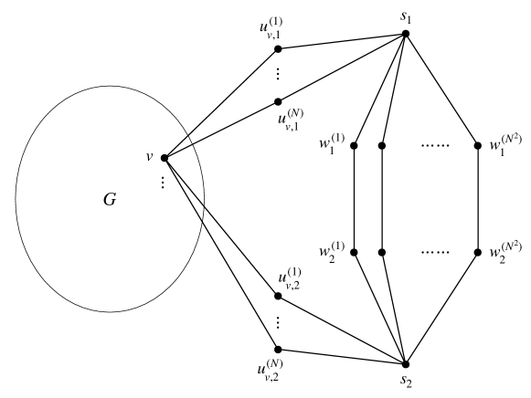
Figure 1: The graph $F$. For every vertex $v\in V_{G}$ and $j\in\{1,2\}$, $v$ and $s_{j}$ are connected by $N$ disjoint paths of length $2$. Also, $s_{1}$ and $s_{2}$ are connected by $N^{2}$ disjoint paths of length $3$.

see Figure 1. Observe that $F$ has $n=4N^{2}+N+2$ vertices. Given two real numbers $\beta_{1},\beta_{2}>0$, we then define an antiferromagnetic Ising model on the graph $F$ as follows:

1. Every edge $\{u,v\}\in E_{G}$ has weight $-0.6$.

2. For every $v\in V_{G}$, $1\leq i\leq N$ and $j=1,2$, the two edges $\{u_{v,j}^{(i)},v\}$ and $\{u_{v,j}^{(i)},s_{j}\}$ have weight $-\beta_{1}$;

3. For every $1\leq i\leq N^{2}$, the edges $\{w_{1}^{(i)},s_{1}\}$, $\{w_{2}^{(i)},s_{2}\}$ and $\{w_{1}^{(i)},w_{2}^{(i)}\}$ have weight $-\beta_{2}$.

We slight abuse of notation, we use $F$ for the resulting Ising model on $F$ and $\mu:=\mu_{F}$ for the corresponding Gibbs distribution. $F$ will be the visible model of our testing instance.

For the hidden model $F^{*}$, we consider the same construction above but replacing $G$ with an independent set $I_{N}$ on $V_{G}$. Let $\mu^{*}:=\mu_{F^{*}}$ be the corresponding the Gibbs distribution. We note first that we can efficiently sample from $\mu^{*}$.

Lemma 3.3.

There is an exact sampling algorithm for the distribution $\mu^{*}$ with running time $\mathrm{poly}(n)$.

Proof.

Configurations in $\Omega_{F^{*}}$ can be classified by their type, which is given by the spins of $s_{1},s_{2}$ and the number of spin $1$’s in the independent set $I_{N}$. There are $4(N+1)$ types in total. Observe that configurations of each type have the same weight by symmetry, and this weight can be computed efficiently since given the spins of $s_{1}$, $s_{2}$ and $I_{N}$ the remaining graph has only isolated vertices and edges. Also it is easy to get the number of configurations of each type. Thus, to sample from $\mu^{*}$, we can first sample a type from the induced distribution on types, and then sample a configuration of the given type uniformly at random. ∎

Our hidden and visible models $F$ and $F^{*}$ are related as follows.

Lemma 3.4.

Let $\varepsilon\in(0,1)$ be a constant, $L=L(n)=\mathrm{poly}(n)$ and $r=96\varepsilon^{-1}\sqrt{\varepsilon L+1}$. Suppose $\hat{Z}\in\mathbb{R}$ is such that $r2^{N}e^{-0.9N}\leq\hat{Z}\leq\frac{1}{r}2^{N}$. Then, for any $\beta_{1}\geq 3$, we can find $0<\beta_{2}<\beta_{1}+2$ in $\mathrm{poly}(n)$ time such that all of the following holds:

1. $\frac{1}{4\sqrt{\varepsilon L+1}}\frac{Z_{G}}{\hat{Z}}\leq\frac{Z_{F}^{\mathrm{D}}}{Z_{F}^{\mathrm{M}}}\leq\frac{1}{\sqrt{\varepsilon L+1}}\frac{Z_{G}}{\hat{Z}}$;

2. $\frac{Z_{F^{*}}^{\mathrm{D}}}{Z_{F^{*}}^{\mathrm{M}}}\leq\frac{1}{r\sqrt{\varepsilon L+1}};$

3. If $Z_{G}\leq\frac{1}{r}\hat{Z}$, then $\left\|\mu-\mu^{*}\right\|_{\textsc{tv}}\leq\frac{1}{16L}$;

4. If $Z_{G}\geq r\hat{Z}$, then $\left\|\mu-\mu^{*}\right\|_{\textsc{tv}}\geq 1-\varepsilon$.

The proof of Lemma 3.4 is provided in Section 3.2. We proceed first with the proof of Theorem 3.2 which follows along the lines of the proof of Theorem 2.5.

Proof of Theorem 3.2.

Consider an antiferromagnetic Ising model on an $N$-vertex $3$-regular graph $G=(V_{G},E_{G})$ with edge weight $\beta_{G}=-0.6$ on every edge and no external field; note that this model belongs to the family $\mathcal{\hat{M}}^{-}_{\textsc{Ising}}(N,3,-0.6,0)$. Let $\hat{Z}>0$ be a real number, let $n=4N^{2}+N+2$ and suppose there is an $\varepsilon$-identity testing algorithm for $\mathcal{M}^{-}_{\textsc{Ising}}(n,n,\beta_{0},0)$ with sample complexity $L=L(n)=\mathrm{poly}(n)$ and running time $\mathrm{poly}(n)$, where $\beta_{0}>0$ is a suitable constant we choose later. Let $r=96\varepsilon^{-1}\sqrt{\varepsilon L+1}$; we want to check whether $Z_{G}\leq\frac{1}{r}\hat{Z}$ or $Z_{G}\geq r\hat{Z}$ where $Z_{G}:=Z_{G,\beta_{G}}$.

We construct the Ising models $F$ and $F^{*}$ with Gibbs distribution $\mu$ and $\mu^{*}$, respectively as described above. We set $\beta_{1}=3$ and use the $\beta_{2}$ supplied by Lemma 3.4; hence the models $F$ and $F^{*}$ belong to $\mathcal{M}^{-}_{\textsc{Ising}}(n,n,\beta_{0},0)$, provided $\beta_{0}\geq\max\{\beta_{1},\beta_{2}\}$.

By Lemma 3.4 when $r2^{N}e^{-0.9N}\leq\hat{Z}\leq\frac{1}{r}2^{N}$, conditions (i) and (ii) from Theorem 2.11 are satisfied; condition (iii) is given by Lemma 3.3. Hence, we have an algorithm for the decision version of $r$-approximate counting for the Ising model on $G$ for $\hat{Z}$ in this range. Otherwise, observe that the weight of every configuration is at least $e^{-0.9N}$, which corresponds to the weight of the monochromatic configuration, and at most $1$. Thus, $2^{N}e^{-0.9N}\leq Z_{G}\leq 2^{N}$. If $\hat{Z}<r2^{N}e^{-0.9N}\leq rZ_{G}$, then we can output $\hat{Z}\leq\frac{1}{r}Z_{G}$. Similarly, $\hat{Z}>\frac{1}{r}2^{N}\geq\frac{1}{r}Z_{G}$ and we output $\hat{Z}\geq rZ_{G}$.

Therefore, we have a $\mathrm{poly}(N)$ running time algorithm for the decision version of $r$-approximate counting for $\mathcal{\hat{M}}^{-}_{\textsc{Ising}}(N,3,-0.6,0)$ where $N=\Theta(n^{1/2})$ and $r=\mathrm{poly}(N)$, as desired. ∎

3.2 Proof of Lemma 3.4

Our construction of the visible and hidden models is inspired by our construction in Section 2.2 for the ferromagnetic Potts model. In particular, the two vertices $\{s_{1},s_{2}\}$ play the role of the complete graph $H$ in our construction in Section 2.2.2. We partition $\Omega_{F}=\{+,-\}^{V_{F}}$ into two disjoint subsets $\Omega_{F}=\Omega_{F}^{\mathrm{M}}\cup\Omega_{F}^{\mathrm{D}}$, depending on whether $\sigma(s_{1})=\sigma(s_{2})$ (the majority phase) or $\sigma(s_{1})\neq\sigma(s_{2})$ (the disordered phase); more precisely, the set of majority configurations is given by

$$\Omega_{F}^{\mathrm{M}}=\left\{\sigma\in\Omega_{F}:\sigma(s_{1})=\sigma(s_{2})\right\}$$

and the set of disordered configurations is

$$\Omega_{F}^{\mathrm{D}}=\left\{\sigma\in\Omega_{F}:\sigma(s_{1})\neq\sigma(s_{2})\right\}.$$

The partition function for the majority phase is defined naturally as

$$Z_{F}^{\mathrm{M}}=\sum_{\sigma\in\Omega_{F}^{\mathrm{M}}}\exp\left(\sum_{\{u,v\}\in E_{F}}\beta_{F}(\{u,v\})\mathbbm{1}\{\sigma(u)=\sigma(v)\}\right),$$

and similarly for $Z_{F}^{\mathrm{D}}$. Therefore, we have $Z_{F}=Z_{F}^{\mathrm{M}}+Z_{F}^{\mathrm{D}}$. In the same way, we also define the partition functions $Z_{F^{*}}^{\mathrm{M}}$ and $Z_{F^{*}}^{\mathrm{D}}$ for the hidden model on the graph $F^{*}$ (notice that $\Omega_{F^{*}}^{\mathrm{M}}=\Omega_{F}^{\mathrm{M}}$ and $\Omega_{F^{*}}^{\mathrm{D}}=\Omega_{F}^{\mathrm{D}}$).

Proof of Lemma 3.4.

Consider the following subset of configurations in $\Omega_{F}^{\mathrm{M}}$ given by

$$\Omega_{F}^{\mathrm{M}_{0}}=\left\{\sigma\in\Omega_{F}^{\mathrm{M}}:\forall v\in V_{G},\sigma(v)=\sigma(s_{1})\right\}.$$

We also define the corresponding partition function $Z_{F}^{\mathrm{M}_{0}}$ and $Z_{F^{*}}^{\mathrm{M}_{0}}$ in the same way as above. We claim that $Z_{F}^{\mathrm{M}_{0}}$ (resp., $Z_{F^{*}}^{\mathrm{M}_{0}}$) is a good approximation (with only exponentially small error) of the partition function $Z_{F}^{\mathrm{M}}$ (resp., $Z_{F^{*}}^{\mathrm{M}}$) that we are interested in.

Claim 3.5.

If $\beta_{1}\geq 3$, then $(1-e^{-2N})Z_{F}^{\mathrm{M}}\leq Z_{F}^{\mathrm{M}_{0}}\leq Z_{F}^{\mathrm{M}}$ and $(1-e^{-2N})Z_{F^{*}}^{\mathrm{M}}\leq Z_{F^{*}}^{\mathrm{M}_{0}}\leq Z_{F^{*}}^{\mathrm{M}}$.

The proof of the following claim is postponed to the end of the section. We then derive explicit formula for $Z_{F}^{\mathrm{D}}$ and $Z_{F}^{\mathrm{M}_{0}}$. For configurations in $\Omega_{F}^{\mathrm{D}}$, every spin assignment to the vertices of $G$, $s_{1}$ and $s_{2}$ is multiplied by a $2e^{-\beta_{1}}(e^{-2\beta_{1}}+1)$ factor, corresponding to the weight of the edges $\{u_{v,j}^{(i)},v\}$, $\{u_{v,j}^{(i)},s_{j}\}$, $j\in\{1,2\}$ for every vertex $v\in V_{G}$ and every $1\leq i\leq N$, and by a $3e^{-2\beta_{2}}+1$ factor for the edges $\{w_{1}^{(i)},s_{1}\}$, $\{w_{2}^{(i)},s_{2}\}$ and $\{w_{1}^{(i)},w_{2}^{(i)}\}$ for every $1\leq i\leq N^{2}$. For configurations in $\Omega_{F}^{\mathrm{M}_{0}}$, each monochromatic configuration on $G$ is multiplied by a $(e^{-2\beta_{1}}+1)^{2}$ factor for the edges $\{u_{v,j}^{(i)},v\}$, $\{u_{v,j}^{(i)},s_{j}\}$, $j\in\{1,2\}$ for every vertex $v\in V_{G}$ and every $1\leq i\leq N$, and by $e^{-3\beta_{2}}+3e^{-\beta_{2}}$ for the edges $\{w_{1}^{(i)},s_{1}\}$, $\{w_{2}^{(i)},s_{2}\}$ and $\{w_{1}^{(i)},w_{2}^{(i)}\}$ for every $1\leq i\leq N^{2}$. Thus, we obtain

$$Z_{F}^{\mathrm{D}} =2\left(3e^{-2\beta_{2}}+1\right)^{N^{2}}\left(2e^{-\beta_{1}}\left(e^{-2\beta_{1}}+1\right)\right)^{N^{2}}Z_{G};$$

$$Z_{F}^{\mathrm{M}_{0}} =2\left(e^{-3\beta_{2}}+3e^{-\beta_{2}}\right)^{N^{2}}\left(e^{-2\beta_{1}}+1\right)^{2N^{2}}e^{-0.9N}.$$

Let $g(x)=(3e^{-2x}+1)/(e^{-3x}+3e^{-x})$ and recall that $\cosh x=\frac{1}{2}(e^{x}+e^{-x})$. We then deduce that

$$\frac{Z_{F}^{\mathrm{D}}}{Z_{F}^{\mathrm{M}_{0}}}=\left(\frac{g(\beta_{2})}{\cosh\beta_{1}}\right)^{N^{2}}e^{0.9N}Z_{G}.$$ (21)

Now for $\beta_{1}\geq 3$, we show that we can pick $\beta_{2}>0$ such that

$$\frac{1}{2\sqrt{\varepsilon L+1}}\frac{e^{-0.9N}}{\hat{Z}}\leq\left(\frac{g(\beta_{2})}{\cosh\beta_{1}}\right)^{N^{2}}\leq\frac{1}{\sqrt{\varepsilon L+1}}\frac{e^{-0.9N}}{\hat{Z}}.$$ (22)

Such $\beta_{2}>0$ always exists and satisfies $\beta_{2}<\beta_{1}+2$. To see this, we note that the function $g(x)$ is a continuous increasing function for $x\geq 0$ with $g(0)=1$ and $g(\infty)=\infty$. Since $\hat{Z}\leq\frac{1}{r}2^{N}$, we get

$$\frac{1}{N^{2}}\log\left(\frac{1}{4\sqrt{\varepsilon L+1}}\,\frac{e^{-0.9N}}{\hat{Z}}\right)+\log(\cosh\beta_{1}) \geq\frac{1}{N^{2}}\log\left(\frac{1}{4\sqrt{\varepsilon L+1}}\,r2^{-N}e^{-0.9N}\right)+\beta_{1}-1$$

$$\geq-\frac{2}{N}+3-1>0,$$

where the second inequality follows from $r/(4\sqrt{\varepsilon L+1})=6/\varepsilon\geq 1$. This shows that

$$\left(\frac{1}{2\sqrt{\varepsilon L+1}}\,\frac{e^{-0.9N}}{\hat{Z}}\right)^{\frac{1}{N^{2}}}\cosh\beta_{1}\geq 1$$

and thus implies the existence of $\beta_{2}>0$. Meanwhile, since $\hat{Z}\geq r2^{N}e^{-0.9N}$ we have

$$\frac{1}{N^{2}}\log\left(\frac{1}{\sqrt{\varepsilon L+1}}\,\frac{e^{-0.9N}}{\hat{Z}}\right)+\log(\cosh\beta_{1})\leq\frac{1}{N^{2}}\log\left(\frac{1}{\sqrt{\varepsilon L+1}}\,\frac{1}{r}2^{-N}\right)+\beta_{1}<\beta_{1},$$

where the second inequality follows from $r\sqrt{\varepsilon L+1}=96\varepsilon^{-1}(\varepsilon L+1)\geq 1$. This shows that

$$e^{\beta_{1}}>g(\beta_{2})=\frac{3e^{-2\beta_{2}}+1}{e^{-3\beta_{2}}+3e^{-\beta_{2}}}\geq\frac{1}{4e^{-\beta_{2}}}\geq e^{\beta_{2}-2}$$

and thus $\beta_{2}<\beta_{1}+2$. Finally, we can compute a $\beta_{2}$ satisfying (22) in $\mathrm{poly}(n)$ time by, for example, the binary search algorithm.

Combining Claim 3.5 and equations (21) and (22), we deduce that

$$\frac{1}{4\sqrt{\varepsilon L+1}}\frac{Z_{G}}{\hat{Z}}\leq(1-e^{-2N})\frac{Z_{F}^{\mathrm{D}}}{Z_{F}^{\mathrm{M}_{0}}}\leq\frac{Z_{F}^{\mathrm{D}}}{Z_{F}^{\mathrm{M}}}\leq\frac{Z_{F}^{\mathrm{D}}}{Z_{F}^{\mathrm{M}_{0}}}\leq\frac{1}{\sqrt{\varepsilon L+1}}\frac{Z_{G}}{\hat{Z}}.$$

This shows the first part of the lemma. For part (ii), we can compute $Z_{F^{*}}^{\mathrm{D}}$ and $Z_{F^{*}}^{\mathrm{M}_{0}}$ in a similar fashion and obtain

$$Z_{F^{*}}^{\mathrm{D}} =2\left(3e^{-2\beta_{2}}+1\right)^{N^{2}}\left(2e^{-\beta_{1}}\left(e^{-2\beta_{1}}+1\right)\right)^{N^{2}}2^{N};$$

$$Z_{F^{*}}^{\mathrm{M}_{0}} =2\left(e^{-3\beta_{2}}+3e^{-\beta_{2}}\right)^{N^{2}}\left(e^{-2\beta_{1}}+1\right)^{2N^{2}}.$$

This gives

$$\frac{Z_{F^{*}}^{\mathrm{D}}}{Z_{F^{*}}^{\mathrm{M}_{0}}}=\left(\frac{g(\beta_{2})}{\cosh\beta_{1}}\right)^{N^{2}}2^{N}.$$ (23)

Therefore, by equations (23) and (22) we obtain

$$\frac{Z_{F^{*}}^{\mathrm{D}}}{Z_{F^{*}}^{\mathrm{M}}}\leq\frac{Z_{F^{*}}^{\mathrm{D}}}{Z_{F^{*}}^{\mathrm{M}_{0}}}\leq\frac{1}{\sqrt{\varepsilon L+1}}\,\frac{e^{-0.9N}}{\hat{Z}}\,2^{N}\leq\frac{1}{r\sqrt{\varepsilon L+1}},$$

where the last inequality follows from the assumption $\hat{Z}\geq r2^{N}e^{-0.9N}$; thus, part (ii) follows.

Next, we derive parts (iii) and (iv). We define $\nu=\mu(\,\cdot\,|\Omega_{F}^{\mathrm{M}})$ to be the distribution conditioned on $\Omega_{F}^{\mathrm{M}}$, and similarly $\nu^{*}=\mu^{*}(\,\cdot\,|\Omega_{F^{*}}^{\mathrm{M}})$. By the definition of total variation distance we have

$$\left\|\mu-\nu\right\|_{\textsc{tv}}=\left\|\mu-\mu(\,\cdot\,|\Omega_{F}^{\mathrm{M}})\right\|_{\textsc{tv}}=\frac{Z_{F}^{\mathrm{D}}}{Z_{F}}=1-\frac{Z_{F}^{\mathrm{M}}}{Z_{F}}.$$

For part (iii), if $Z_{G}\leq\frac{1}{r}\hat{Z}$, then we deduce from part (i) that

$$\left\|\mu-\nu\right\|_{\textsc{tv}}\leq\frac{Z_{F}^{\mathrm{D}}}{Z_{F}^{\mathrm{M}}}\leq\frac{1}{\sqrt{\varepsilon L+1}}\frac{Z_{G}}{\hat{Z}}\leq\frac{1}{r\sqrt{\varepsilon L+1}}=\frac{\varepsilon}{96(\varepsilon L+1)}\leq\frac{1}{96L}.$$

Similarly, part (ii) implies

$$\left\|\mu^{*}-\nu^{*}\right\|_{\textsc{tv}}\leq\frac{Z_{F^{*}}^{\mathrm{D}}}{Z_{F^{*}}^{\mathrm{M}}}\leq\frac{1}{r\sqrt{\varepsilon L+1}}=\frac{\varepsilon}{96(\varepsilon L+1)}\leq\min\left\{\frac{1}{96L},\frac{\varepsilon}{96}\right\}.$$

Let $\rho=\nu(\,\cdot\,|\Omega_{F}^{\mathrm{M}_{0}})$ denote the conditional distribution of $\nu$ on $\Omega_{F}^{\mathrm{M}_{0}}$. Observe that $\rho$ does not depend on the graph $G$, because we condition on the event that all vertices from $G$ receive the same spin, and thus the structure of $G$ does not affect the conditional distribution $\rho$. In particular, we have $\rho=\nu(\,\cdot\,|\Omega_{F}^{\mathrm{M}_{0}})=\nu^{*}(\,\cdot\,|\Omega_{F^{*}}^{\mathrm{M}_{0}})$. Then, Claim 3.5 implies that

$$\left\|\nu-\rho\right\|_{\textsc{tv}}=1-\frac{Z_{F}^{\mathrm{M}_{0}}}{Z_{F}^{\mathrm{M}}}\leq e^{-2N}$$

and similarly $\left\|\nu^{*}-\rho\right\|_{\textsc{tv}}\leq e^{-2N}$. Therefore, we obtain from the triangle inequality that

$$\left\|\nu-\nu^{*}\right\|_{\textsc{tv}}\leq\left\|\nu-\rho\right\|_{\textsc{tv}}+\left\|\nu^{*}-\rho\right\|_{\textsc{tv}}\leq 2e^{-2N}.$$

We conclude again from the triangle inequality that

$$\left\|\mu-\mu^{*}\right\|_{\textsc{tv}}\leq\left\|\mu-\nu\right\|_{\textsc{tv}}+\left\|\mu^{*}-\nu^{*}\right\|_{\textsc{tv}}+\left\|\nu-\nu^{*}\right\|_{\textsc{tv}}\leq\frac{1}{96L}+\frac{1}{96L}+2e^{-2N}\leq\frac{1}{16L}.$$

Finally, for part (iv), if $Z_{G}\geq r\hat{Z}$, then by part (ii) we have

$$\left\|\mu-\nu\right\|_{\textsc{tv}}\geq 1-\frac{Z_{F}^{\mathrm{M}}}{Z_{F}^{\mathrm{D}}}\geq 1-4\sqrt{\varepsilon L+1}\,\frac{\hat{Z}}{Z_{G}}\geq 1-\frac{4}{r}\sqrt{\varepsilon L+1}=1-\frac{\varepsilon}{24}.$$

Hence,

$$\left\|\mu-\mu^{*}\right\|_{\textsc{tv}}\geq\left\|\mu-\nu\right\|_{\textsc{tv}}-\left\|\mu^{*}-\nu^{*}\right\|_{\textsc{tv}}-\left\|\nu-\nu^{*}\right\|_{\textsc{tv}}\geq 1-\frac{\varepsilon}{24}-\frac{\varepsilon}{96}-2e^{-2N}\geq 1-\varepsilon,$$

as claimed. ∎

Proof of Claim 3.5.

For the first inequality, note that $Z_{F}^{\mathrm{M}_{0}}\leq Z_{F}^{\mathrm{M}}$. A union bound implies

$$1-\frac{Z_{F}^{\mathrm{M}_{0}}}{Z_{F}^{\mathrm{M}}} =\Pr\Big{(}\exists v\in V_{G}:\sigma(v)\neq\sigma(s_{1})\Big{|}\sigma(s_{1})=\sigma(s_{2})\Big{)}\leq\sum_{v\in V_{G}}\Pr(\sigma(v)\neq\sigma(s_{1})|\sigma(s_{1})=\sigma(s_{2})).$$

For every $\sigma\in\Omega_{F}^{\mathrm{M}}$ and $v\in V_{G}$, if $\sigma(v)\neq\sigma(s_{1})$, then the total weight of edges incident to $v$ is at most $(2e^{-\beta_{1}})^{2N}$; and if $\sigma(v)=\sigma(s_{1})$, then it is at least $(e^{-2\beta_{1}}+1)^{2N}\exp(\beta_{G}\deg_{G}(v))\geq(e^{-2\beta_{1}}+1)^{2N}e^{-1.8}$. Thus, we get

$$\Pr(\sigma(v)\neq\sigma(s_{1})|\sigma(s_{1})=\sigma(s_{2})) \leq\frac{(2e^{-\beta_{1}})^{2N}}{(2e^{-\beta_{1}})^{2N}+(e^{-2\beta_{1}}+1)^{2N}e^{-1.8}}$$

$$\leq e^{1.8}\left(\frac{2e^{-\beta_{1}}}{e^{-2\beta_{1}}+1}\right)^{2N}\leq 10e^{-2(\beta_{1}-1)N}\leq 10e^{-4N},$$

where the last inequality follows from the assumption $\beta_{1}\geq 3$. Therefore,

$$\frac{Z_{F}^{\mathrm{M}_{0}}}{Z_{F}^{\mathrm{M}}}\geq 1-10Ne^{-4N}\geq 1-e^{-2N}.$$

The bound for $F^{*}$ can be derived analogously. ∎

4 Testing ferromagnetic RBMs with inconsistent fields

In this section, we establish our lower bound for identity testing for ferromagnetic RBMs with inconsistent fields; specifically, we prove Theorem 1.2 from the introduction. Let us formally define first the notions of consistent and inconsistent external fields.

Definition 4.1.

Consider an Ising model on a graph $G=(V_{G},E_{G})$ with external field $h_{G}:V_{G}\times\{1,2\}\rightarrow\mathbb{R}$. We say that the external field $h_{G}$ is consistent if  $\forall v\in V_{G}$, $h_{G}(v,1)\geq 0$ and $h_{G}(v,2)=0$ or $\forall v\in V_{G}$, $h_{G}(v,2)\geq 0$ and $h_{G}(v,1)=0$.

We use once again our reduction strategy from $r$-approximate counting to testing. We start from the following well-known result.

Theorem 4.2 (​[25]).

There is no $\mathsf{FPRAS}$ for the partition function of ferromagnetic Ising models with inconsistent fields, unless #BIS admits an $\mathsf{FPRAS}$.

The next step is the reduction from the decision version of approximate counting to identity testing.

Theorem 4.3.

Let $\varepsilon\in(0,1)$ be any constant. For every $\hat{\beta},\hat{h}>0$ there exist $\beta_{0},h_{0}>0$ such that an $\varepsilon$-identity testing algorithm for $\mathcal{M}^{+}_{\textsc{Ising}}(n,n,\beta_{0},h_{0})$ with $\mathrm{poly}(n)$ sample complexity and running time can be used to solve the decision $r$-approximate counting problem for $\mathcal{\hat{M}}^{+}_{\textsc{Ising}}(N,N,\hat{\beta},\hat{h})$ in $\mathrm{poly}(N)$ time, where $N=\Theta(\sqrt{n})$ and $r=\mathrm{poly}(N)$.

We can now provide the proof of Theorem 1.2.

Proof of Theorem 1.2.

Follows from Theorems 4.2, 2.4, 4.3 and 5.2. ∎

4.1 Reducing counting to testing for the ferromagnetic Ising model with an inconsistent field: proof of Theorem 4.3

Testing instance construction.  Consider an instance $(G,\beta_{G},h_{G})$ of ferromagnetic Ising models with an inconsistent field, where $G=(V_{G},E_{G})$ is the underlying graph with $N=|V_{G}|$, $\beta_{G}(e)=\hat{\beta}>0$ for every $e\in E_{G}$, and at every vertex the external field is either $h_{G}=(\hat{h},0)$ or $h_{G}=(0,\hat{h})$ for $\hat{h}>0$; that is, $\forall v\in V_{G},~{}h_{G}(v,j)=\mathbbm{1}(j=1)\hat{h}$ for $j=\{1,2\}$ or $h_{G}(v,j)=\mathbbm{1}(i=2)\hat{h}$ for $i=\{1,2\}$. Note that for consistency with the notation in the previous sections we use spins $\{1,2\}$ for the Ising model, instead of the usual “$+$” and “$-$” spins. Our goal is to give a $r$-approximate counting algorithm for the partition function $Z_{G}:=Z_{G,\beta_{G},h_{G}}$ for some $r=\mathrm{poly}(N)$ using an identity testing algorithm.

Define $F$ to be a graph with the vertex set

$$V_{F}=V_{G}\cup\{s_{1},s_{2}\}\cup\left\{u^{(i)}_{v,j}:v\in V_{G},1\leq i\leq N,j\in\{1,2\}\right\}\cup\left\{w^{(i)}_{j}:1\leq i\leq N^{2},j\in\{1,2\}\right\}$$

and the edge set

$$E_{F}={} E_{G}\cup\left\{\{u_{v,j}^{(i)},v\},\{u_{v,j}^{(i)},s_{j}\}:v\in V_{G},1\leq i\leq N,j\in\{1,2\}\right\}$$

$$\cup\left\{\{w_{j}^{(i)},s_{j}\}:1\leq i\leq N^{2},j\in\{1,2\}\right\};$$

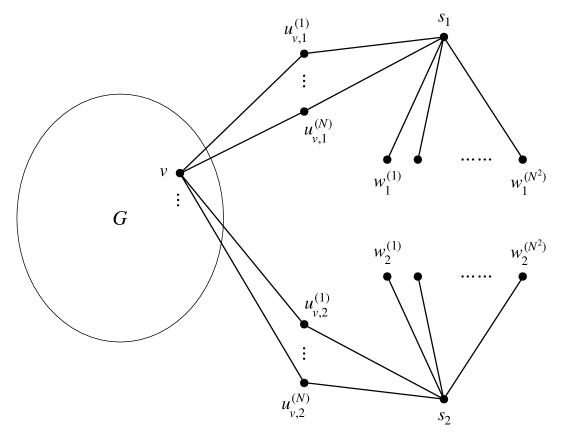
Figure 2: The graph $F$. For every vertex $v\in V_{G}$ and $j\in\{1,2\}$, $v$ and $s_{j}$ are connected by $N$ disjoint paths of length $2$. Also, each of $s_{1}$ and $s_{2}$ is adjacent to $N^{2}$ vertices with nonzero fields.

see Figure 2.

Given three real numbers $\beta_{1},\beta_{2},h>0$, we then define a ferromagnetic Ising model on the graph $F$ as follows:

1. Every edge $\{u,v\}\in E_{G}$ has weight $\hat{\beta}$ and every vertex $v\in V_{G}$ has external field given by $h_{G}$.

2. For every $v\in V_{G}$, $1\leq i\leq N$ and $j\in\{1,2\}$, the two edges $\{u_{v,j}^{(i)},v\}$ and $\{u_{v,j}^{(i)},s_{j}\}$ have weight $\beta_{1}$;

3. For every $1\leq i\leq N^{2}$ and $j\in\{1,2\}$, the edge $\{w_{j}^{(i)},s_{j}\}$ has weight $\beta_{2}$;

4. For every $1\leq i\leq N^{2}$, the vertex $w_{1}^{(i)}$ has external field $(h,0)$ and the vertex $w_{2}^{(i)}$ has external field $(0,h)$; that is, $h_{F}(w_{1}^{(i)},j)=\mathbbm{1}(j=1)h$ and $h_{F}(w_{2}^{(i)},j)=\mathbbm{1}(j=2)h$.

Thus, $F$ is a graph on $n=4N^{2}+N+2$ vertices and the Ising model on $F$ is ferromagnetic with an inconsistent external field. Let $\mu:=\mu_{F}$ denote the corresponding Gibbs distribution.

For the hidden model $F^{*}$, we consider the same construction above but replacing $G$ with a complete graph $K=K_{N}$ on $N$ vertices where every edge has weight $\beta_{K}=\hat{\beta}+4\log 2>0$ and every vertex has the same field $h_{G}$ as the Ising model on $G$. Let $\mu^{*}:=\mu_{F^{*}}$ be the corresponding the Gibbs distribution. We note first that we can efficiently sample from $\mu^{*}$.

Lemma 4.4.

There is an exact sampling algorithm for the distribution $\mu^{*}$ with running time $\mathrm{poly}(n)$.

Proof.

Configurations in $\Omega_{F^{*}}$ are classified by their type, which is given by the spins of the vertices $s_{1}$ and $s_{2}$ and the number of vertices with spin $1$ in the complete graph $K_{N}$. There are $4(N+1)$ types in total. Observe that configurations of each type have the same weight by symmetry, and this weight can be computed efficiently since given the spins of $s_{1}$, $s_{2}$ and $K_{N}$ the remaining graph has only isolated vertices and edges. It is also straightforward to get the number of configurations of each type. Thus, to sample from $\mu^{*}$, we first sample a type from the induced distribution on the types, and then sample a configuration of the given type uniformly at random. ∎

Denote the sum of weights of two monochromatic configurations on $G$ by

$$Z_{G}^{\mathrm{mo}}:=\sum_{i\in\{1,2\}}\exp\left(\hat{\beta}|E_{G}|+\sum_{v\in V_{G}}h_{G}(v,i)\right).$$

The hidden and visible models $F$ and $F^{*}$ are related as follows.

Lemma 4.5.

Let $\varepsilon\in(0,1)$ be a constant, $L=L(n)=\mathrm{poly}(n)$ and $r=96\varepsilon^{-1}\sqrt{\varepsilon L+1}$. Suppose $\hat{Z}\in\mathbb{R}$ is such that $rZ_{G}^{\mathrm{mo}}\leq\hat{Z}\leq\frac{1}{r}\exp(\frac{1}{2}(\hat{\beta}+\hat{h}+1)N^{2})$. Then, for any $\beta_{1}\geq\frac{1}{2}(\hat{\beta}+\hat{h}+5)$, we can find $\beta_{2}\in(0,\beta_{1})$ in $\mathrm{poly}(n)$ time such that by setting $h=\beta_{2}$ al of the following holds:

1. $\frac{1}{4\sqrt{\varepsilon L+1}}\frac{Z_{G}}{\hat{Z}}\leq\frac{Z_{F}^{\mathrm{D}}}{Z_{F}^{\mathrm{M}}}\leq\frac{1}{\sqrt{\varepsilon L+1}}\frac{Z_{G}}{\hat{Z}}$;

2. $\frac{Z_{F^{*}}^{\mathrm{D}}}{Z_{F^{*}}^{\mathrm{M}}}\leq\frac{2}{r\sqrt{\varepsilon L+1}}$;

3. If $Z_{G}\leq\frac{1}{r}\hat{Z}$, then $\left\|\mu-\mu^{*}\right\|_{\textsc{tv}}\leq\frac{1}{16L}$;

4. If $Z_{G}\geq r\hat{Z}$, then $\left\|\mu-\mu^{*}\right\|_{\textsc{tv}}\geq 1-\varepsilon$.

The proof of Lemma 4.5 is provided in Section 4.2. We provide next the proof of Theorem 4.3.

Proof of Theorem 4.3.

Consider the ferromagnetic Ising model $(G,\beta_{G},h_{G})$, where $G=(V_{G},E_{G})$ is an $N$-vertex graph, $\beta_{G}(e)=\hat{\beta}$ for all $e\in E_{G}$ and $h_{G}(v,j)=\mathbbm{1}(j=1)\hat{h}$ for $j=\{1,2\}$ or $h_{G}(v,j)=\mathbbm{1}(j=2)\hat{h}$ for $i=\{1,2\}$ for all $v\in V_{G}$; note that this model belongs to $\mathcal{\hat{M}}^{+}_{\textsc{Ising}}(N,N,\hat{\beta},\hat{h})$. Let $\hat{Z}>0$ be a real number, let $n=4N^{2}+N+2$ and suppose there is an $\varepsilon$-identity testing algorithm for $\mathcal{M}^{+}_{\textsc{Ising}}(n,n,\beta_{0},h_{0})$ with sample complexity $L=L(n)=\mathrm{poly}(n)$ and running time $\mathrm{poly}(n)$, where $\beta_{0},h_{0}>0$ are a suitable constants. Let $r=96\varepsilon^{-1}\sqrt{\varepsilon L+1}$; we want to check whether $Z_{G}\leq\frac{1}{r}\hat{Z}$ or $Z_{G}\geq r\hat{Z}$ where $Z_{G}:=Z_{G,\beta_{G},h_{G}}$.

We construct the Ising models $F$ and $F^{*}$ with Gibbs distribution $\mu$ and $\mu^{*}$, respectively as described above, setting $\beta_{1}=\frac{1}{2}(\hat{\beta}+\hat{h}+5)$, using the $\beta_{2}$ supplied by Lemma 4.5, and taking $h=\beta_{2}$; hence the models $F$ and $F^{*}$ belong to $\mathcal{M}^{+}_{\textsc{Ising}}(n,n,\beta_{0},h_{0})$, provided $\beta_{0}\geq\max\{\hat{\beta},\beta_{K},\beta_{1},\beta_{2}\}$ and $h_{0}\geq\max\{\hat{h},h\}$.

By Lemma 4.5 when $rZ_{G}^{\mathrm{mo}}\leq\hat{Z}\leq\frac{1}{r}\exp(\frac{1}{2}(\hat{\beta}+\hat{h}+1)N^{2})$, conditions (i) and (ii) of Theorem 2.11 are satisfied; condition (iii) is given by Lemma 4.4. Therefore, we have an algorithm for the decision version of $r$-approximate counting for the Ising model on $G$ for $\hat{Z}$ in this range. When $\hat{Z}$ is not in this range, note that we have the following crude bounds on $Z_{G}$:

$$Z_{G}^{\mathrm{mo}}\leq Z_{G}\leq 2^{N}\cdot\exp\left(\hat{\beta}\frac{N^{2}}{2}+\hat{h}N\right)\leq\exp\left(\frac{1}{2}(\hat{\beta}+\hat{h}+1)N^{2}\right).$$

Thus, if $\hat{Z}<rZ_{G}^{\mathrm{mo}}\leq rZ_{G}$ we can output $\hat{Z}\leq\frac{1}{r}Z_{G}$. Similarly, $\hat{Z}>\frac{1}{r}\exp(\frac{1}{2}(\hat{\beta}+\hat{h}+1)N^{2})\geq\frac{1}{r}Z_{G}$ we output $\hat{Z}\geq rZ_{G}$.

Therefore, we have a $\mathrm{poly}(N)$ running time algorithm for the decision version of $r$-approximate counting for $\mathcal{\hat{M}}^{+}_{\textsc{Ising}}(N,N,\hat{\beta},\hat{h})$ where $N=\Theta(n^{1/2})$ and $r=\mathrm{poly}(N)$, as desired. ∎

4.2 Proof of Lemma 4.5

We reuse the notation introduce in Section 3.2. Recall that $\Omega_{F}^{\mathrm{M}}=\{\sigma\in\Omega_{F}:\sigma(s_{1})=\sigma(s_{2})\}$ and $\Omega_{F}^{\mathrm{D}}=\{\sigma\in\Omega_{F}:\sigma(s_{1})\neq\sigma(s_{2})\}$. Also the partition function for the majority phase is given by

$$Z_{F}^{\mathrm{M}}=\sum_{\sigma\in\Omega_{F}^{\mathrm{M}}}\exp\left(\sum_{\{u,v\}\in E_{F}}\beta_{F}(\{u,v\})\mathbbm{1}\{\sigma(u)=\sigma(v)\}+\sum_{v\in V_{F}}h_{F}(v,\sigma(v))\right)$$

and $Z_{F}^{\mathrm{D}}$ is defined similarly. The corresponding partition functions for the hidden model are denoted by $Z_{F^{*}}^{\mathrm{M}}$ and $Z_{F^{*}}^{\mathrm{D}}$.

Proof.

Let $\Omega_{F}^{\mathrm{M}_{0}}=\left\{\sigma\in\Omega_{F}^{\mathrm{M}}:\forall v\in V_{G},\sigma(v)=\sigma(s_{1})\right\}$ and consider restrictions of partition functions $Z_{F}^{\mathrm{M}_{0}}$ and $Z_{F^{*}}^{\mathrm{M}_{0}}$, as in the proof of Lemma 3.4. The following claim, whose proof is provided at the end of the section, has the same flavor as Claim 3.5.

Claim 4.6.

If $\beta_{1}\geq\frac{1}{2}(\hat{\beta}+\hat{h}+5)$, then $(1-e^{-2N})Z_{F}^{\mathrm{M}}\leq Z_{F}^{\mathrm{M}_{0}}\leq Z_{F}^{\mathrm{M}}$ and $(1-e^{-2N})Z_{F^{*}}^{\mathrm{M}}\leq Z_{F^{*}}^{\mathrm{M}_{0}}\leq Z_{F^{*}}^{\mathrm{M}}$.

We then derive explicit formulae for the two partition functions $Z_{F}^{\mathrm{D}}$ and $Z_{F}^{\mathrm{M}_{0}}$. For configurations $\sigma\in\Omega_{F}^{\mathrm{D}}$ with $\sigma(s_{1})=1$ and $\sigma(s_{2})=2$ (resp., $\sigma(s_{1})=2$ and $\sigma(s_{2})=1$), the weight of the configuration on $G$ is multiply by a factor of $2e^{\beta_{1}}(e^{2\beta_{1}}+1)$ for each edge $\{u_{v,j}^{(i)},v\}$, $\{u_{v,j}^{(i)},s_{j}\}$, $j\in\{1,2\}$ for every $v\in V_{G}$ and every $1\leq i\leq N$; it is also multiply by a $(e^{\beta_{2}+h}+1)^{2}$ (resp., $(e^{\beta_{2}}+e^{h})^{2}$) factor for each edge $\{w_{j}^{(i)},s_{j}\}$ and the vertex $w_{j}^{(i)}$, $j=\{1,2\}$ and $1\leq i\leq N^{2}$. For configurations in $\Omega_{F}^{\mathrm{M}_{0}}$, both monochromatic configurations on $G$ receive additional weight $(e^{2\beta_{1}}+1)^{2}$ for the edges $\{u_{v,j}^{(i)},v\}$, $\{u_{v,j}^{(i)},s_{j}\}$, $j=\{1,2\}$ for every vertex $v\in V_{G}$ and every $1\leq i\leq N$, and a $(e^{\beta_{2}+h}+1)(e^{\beta_{2}}+e^{h})$ factor for each edge $\{w_{j}^{(i)},s_{j}\}$ and the vertex $w_{j}^{(i)}$, $j=\{1,2\}$ for every $1\leq i\leq N^{2}$. Thus, we obtain that

$$Z_{F}^{\mathrm{D}} =\left[\left(e^{\beta_{2}+h}+1\right)^{2N^{2}}+\left(e^{\beta_{2}}+e^{h}\right)^{2N^{2}}\right]\left(2e^{\beta_{1}}\left(e^{2\beta_{1}}+1\right)\right)^{N^{2}}Z_{G};$$

$$Z_{F}^{\mathrm{M}_{0}} =\left(e^{\beta_{2}+h}+1\right)^{N^{2}}\left(e^{\beta_{2}}+e^{h}\right)^{N^{2}}\left(e^{2\beta_{1}}+1\right)^{2N^{2}}Z_{G}^{\mathrm{mo}}.$$

Recall that $\cosh x=\frac{1}{2}(e^{x}+e^{-x})$. We then deduce that

$$\frac{Z_{F}^{\mathrm{D}}}{Z_{F}^{\mathrm{M}_{0}}}=\left[\left(\frac{\cosh(\frac{\beta_{2}+h}{2})}{\cosh(\frac{\beta_{2}-h}{2})}\right)^{N^{2}}+\left(\frac{\cosh(\frac{\beta_{2}-h}{2})}{\cosh(\frac{\beta_{2}+h}{2})}\right)^{N^{2}}\right]\left(\frac{1}{\cosh\beta_{1}}\right)^{N^{2}}\frac{Z_{G}}{Z_{G}^{\mathrm{mo}}}.$$

Since $\cosh x\geq 1$ for all $x\in\mathbb{R}$, let $h=\beta_{2}>0$ and then we get

$$\left(\frac{\cosh\beta_{2}}{\cosh\beta_{1}}\right)^{N^{2}}\frac{Z_{G}}{Z_{G}^{\mathrm{mo}}}\leq\frac{Z_{F}^{\mathrm{D}}}{Z_{F}^{\mathrm{M}_{0}}}\leq 2\left(\frac{\cosh\beta_{2}}{\cosh\beta_{1}}\right)^{N^{2}}\frac{Z_{G}}{Z_{G}^{\mathrm{mo}}}.$$ (24)

Now for $\beta_{1}\geq\frac{1}{2}(\hat{\beta}+\hat{h}+5)$, we pick $\beta_{2}>0$ such that

$$\frac{1}{3\sqrt{\varepsilon L+1}}\,\frac{Z_{G}^{\mathrm{mo}}}{\hat{Z}}\leq\left(\frac{\cosh\beta_{2}}{\cosh\beta_{1}}\right)^{N^{2}}\leq\frac{1}{2\sqrt{\varepsilon L+1}}\,\frac{Z_{G}^{\mathrm{mo}}}{\hat{Z}},$$ (25)

Such $\beta_{2}>0$ always exists and satisfies $\beta_{2}<\beta_{1}$. To see this, we note that since $\hat{Z}\leq\frac{1}{r}\exp(\frac{1}{2}(\hat{\beta}+\hat{h}+1)N^{2})$ and $Z_{G}^{\mathrm{mo}}\geq 2$, we have

$$\frac{1}{N^{2}}\log\left(\frac{1}{3\sqrt{\varepsilon L+1}}\,\frac{Z_{G}^{\mathrm{mo}}}{\hat{Z}}\right)+\log(\cosh\beta_{1}) \geq\frac{1}{N^{2}}\log\left(\frac{1}{3\sqrt{\varepsilon L+1}}\,2re^{-\frac{1}{2}(\hat{\beta}+\hat{h}+1)N^{2}}\right)+\beta_{1}-1$$

$$\geq-\frac{1}{2}(\hat{\beta}+\hat{h}+1)+\frac{1}{2}(\hat{\beta}+\hat{h}+5)-1=1>0,$$

where the second inequality follows from $2r/(3\sqrt{\varepsilon L+1})=64/\varepsilon\geq 1$. This is equivalent to

$$\left(\frac{1}{3\sqrt{\varepsilon L+1}}\,\frac{Z_{G}^{\mathrm{mo}}}{\hat{Z}}\right)^{\frac{1}{N^{2}}}\cosh\beta_{1}\geq 1,$$

and hence $\beta_{2}>0$ satisfying (25) always exists and can be computed in $\mathrm{poly}(n)$ time. Note also that since $\hat{Z}\geq rZ_{G}^{\mathrm{mo}}$ we have

$$\frac{1}{2\sqrt{\varepsilon L+1}}\,\frac{Z_{G}^{\mathrm{mo}}}{\hat{Z}}\leq\frac{1}{2r\sqrt{\varepsilon L+1}}=\frac{\varepsilon}{192(\varepsilon L+1)}<1.$$

This shows that $\cosh\beta_{2}/\cosh\beta_{1}<1$ and thus $\beta_{2}<\beta_{1}$.

Combining Claim 4.6 and inequalities (24) and (25), we deduce that

$$\frac{1}{4\sqrt{\varepsilon L+1}}\frac{Z_{G}}{\hat{Z}}\leq(1-e^{-2N})\frac{Z_{F}^{\mathrm{D}}}{Z_{F}^{\mathrm{M}_{0}}}\leq\frac{Z_{F}^{\mathrm{D}}}{Z_{F}^{\mathrm{M}}}\leq\frac{Z_{F}^{\mathrm{D}}}{Z_{F}^{\mathrm{M}_{0}}}\leq\frac{1}{\sqrt{\varepsilon L+1}}\frac{Z_{G}}{\hat{Z}}.$$

This shows part (i). For part (ii), we can compute $Z_{F^{*}}^{\mathrm{D}}/Z_{F^{*}}^{\mathrm{M}_{0}}$ in a similar fashion and obtain

$$\left(\frac{\cosh\beta_{2}}{\cosh\beta_{1}}\right)^{N^{2}}\frac{Z_{K}}{Z_{K}^{\mathrm{mo}}}\leq\frac{Z_{F^{*}}^{\mathrm{D}}}{Z_{F^{*}}^{\mathrm{M}_{0}}}\leq 2\left(\frac{\cosh\beta_{2}}{\cosh\beta_{1}}\right)^{N^{2}}\frac{Z_{K}}{Z_{K}^{\mathrm{mo}}}.$$ (26)

Therefore, by inequalities (26) and (25) we obtain

$$\frac{Z_{F^{*}}^{\mathrm{D}}}{Z_{F^{*}}^{\mathrm{M}}}\leq\frac{Z_{F^{*}}^{\mathrm{D}}}{Z_{F^{*}}^{\mathrm{M}_{0}}}\leq\frac{1}{\sqrt{\varepsilon L+1}}\,\frac{Z_{G}^{\mathrm{mo}}}{\hat{Z}}\frac{Z_{K}}{Z_{K}^{\mathrm{mo}}}\leq\frac{2}{r\sqrt{\varepsilon L+1}},$$

where the last inequality follows from the assumption $\hat{Z}\geq rZ_{G}^{\mathrm{mo}}$ and the fact that $Z_{K}^{\mathrm{mo}}/Z_{K}\geq 1/2$ when $\beta_{K}\geq 4\log 2$. Thus, part (ii) is established.

To establish part (iii), let us define $\nu=\mu(\,\cdot\,|\Omega_{F}^{\mathrm{M}})$ to be the distribution conditioned on $\Omega_{F}^{\mathrm{M}}$, and similarly $\nu^{*}=\mu^{*}(\,\cdot\,|\Omega_{F^{*}}^{\mathrm{M}})$. By the definition of total variation distance we have

$$\left\|\mu-\nu\right\|_{\textsc{tv}}=\left\|\mu-\mu(\,\cdot\,|\Omega_{F}^{\mathrm{M}})\right\|_{\textsc{tv}}=\frac{Z_{F}^{\mathrm{D}}}{Z_{F}}=1-\frac{Z_{F}^{\mathrm{M}}}{Z_{F}}.$$

For part (iii), if $Z_{G}\leq\frac{1}{r}\hat{Z}$, we deduce from part (i) that

$$\left\|\mu-\nu\right\|_{\textsc{tv}}\leq\frac{Z_{F}^{\mathrm{D}}}{Z_{F}^{\mathrm{M}}}\leq\frac{1}{\sqrt{\varepsilon L+1}}\frac{Z_{G}}{\hat{Z}}\leq\frac{1}{r\sqrt{\varepsilon L+1}}=\frac{\varepsilon}{96(\varepsilon L+1)}\leq\frac{1}{96L}.$$

Similarly, by part (ii) we have

$$\left\|\mu^{*}-\nu^{*}\right\|_{\textsc{tv}}\leq\frac{Z_{F^{*}}^{\mathrm{D}}}{Z_{F^{*}}^{\mathrm{M}}}\leq\frac{2}{r\sqrt{\varepsilon L+1}}=\frac{\varepsilon}{48(\varepsilon L+1)}\leq\min\left\{\frac{1}{48L},\frac{\varepsilon}{48}\right\}.$$

Let $\rho=\nu(\,\cdot\,|\Omega_{F}^{\mathrm{M}_{0}})$ denote the conditional distribution of $\nu$ on $\Omega_{F}^{\mathrm{M}_{0}}$. Observe that $\rho$ does not depend on the graph $G$, because we condition on the event that all vertices from $G$ receive the same spin, and thus the structure of $G$ does not affect the conditional distribution $\rho$. In particular, we have $\rho=\nu(\,\cdot\,|\Omega_{F}^{\mathrm{M}_{0}})=\nu^{*}(\,\cdot\,|\Omega_{F^{*}}^{\mathrm{M}_{0}})$. Then, Claim 4.6 implies that

$$\left\|\nu-\rho\right\|_{\textsc{tv}}=1-\frac{Z_{F}^{\mathrm{M}_{0}}}{Z_{F}^{\mathrm{M}}}\leq e^{-2N}$$

and similarly $\left\|\nu^{*}-\rho\right\|_{\textsc{tv}}\leq e^{-2N}$. Therefore, we obtain from the triangle inequality that

$$\left\|\nu-\nu^{*}\right\|_{\textsc{tv}}\leq\left\|\nu-\rho\right\|_{\textsc{tv}}+\left\|\nu^{*}-\rho\right\|_{\textsc{tv}}\leq 2e^{-2N}.$$

We conclude again from the triangle inequality that

$$\left\|\mu-\mu^{*}\right\|_{\textsc{tv}}\leq\left\|\mu-\nu\right\|_{\textsc{tv}}+\left\|\mu^{*}-\nu^{*}\right\|_{\textsc{tv}}+\left\|\nu-\nu^{*}\right\|_{\textsc{tv}}\leq\frac{1}{96L}+\frac{1}{48L}+2e^{-2N}\leq\frac{1}{16L}.$$

For part (iv), if $Z_{G}\geq r\hat{Z}$, then by part (i)

$$\left\|\mu-\nu\right\|_{\textsc{tv}}\geq 1-\frac{Z_{F}^{\mathrm{M}}}{Z_{F}^{\mathrm{D}}}\geq 1-4\sqrt{\varepsilon L+1}\,\frac{\hat{Z}}{Z_{G}}\geq 1-\frac{4}{r}\sqrt{\varepsilon L+1}=1-\frac{\varepsilon}{24}.$$

Hence,

$$\left\|\mu-\mu^{*}\right\|_{\textsc{tv}}\geq\left\|\mu-\nu\right\|_{\textsc{tv}}-\left\|\mu^{*}-\nu^{*}\right\|_{\textsc{tv}}-\left\|\nu-\nu^{*}\right\|_{\textsc{tv}}\geq 1-\frac{\varepsilon}{24}-\frac{\varepsilon}{48}-2e^{-2N}\geq 1-\varepsilon,$$

as claimed. ∎

Proof of Claim 4.6.

Note first that $Z_{F}^{\mathrm{M}_{0}}\leq Z_{F}^{\mathrm{M}}$ and from a union bound we get

$$1-\frac{Z_{F}^{\mathrm{M}_{0}}}{Z_{F}^{\mathrm{M}}} =\Pr\Big{(}\exists v\in V_{G}:\sigma(v)\neq\sigma(s_{1})\Big{|}\sigma(s_{1})=\sigma(s_{2})\Big{)}\leq\sum_{v\in V_{G}}\Pr(\sigma(v)\neq\sigma(s_{1})|\sigma(s_{1})=\sigma(s_{2})).$$

For every $\sigma\in\Omega_{F}^{\mathrm{M}}$ and $v\in V_{G}$, if $\sigma(v)\neq\sigma(s_{1})$, then the total weight of edges incident to $v$ is at most $(2e^{\beta_{1}})^{2N}\exp(\hat{\beta}(N-1)+\hat{h})$; and if $\sigma(v)=\sigma(s_{1})$, then it is at least $(e^{2\beta_{1}}+1)^{2N}$. Thus, we get

$$\Pr(\sigma(v)\neq\sigma(s_{1})|\sigma(s_{1})=\sigma(s_{2})) \leq\frac{(2e^{\beta_{1}})^{2N}\exp(\hat{\beta}(N-1)+\hat{h})}{(2e^{\beta_{1}})^{2N}\exp(\hat{\beta}(N-1)+\hat{h})+(e^{2\beta_{1}}+1)^{2N}}$$

$$\leq\left(\frac{2e^{\beta_{1}}}{e^{2\beta_{1}}+1}\right)^{2N}\exp\left(\hat{\beta}(N-1)+\hat{h}\right)$$

$$\leq\exp\left(-2(\beta_{1}-1)N\right)\cdot\exp\left((\hat{\beta}+\hat{h})N\right)$$

$$\leq e^{-3N}.$$

where the last inequality follows from the assumption $\beta_{1}\geq\frac{1}{2}(\hat{\beta}+\hat{h}+5)$. Therefore, $\frac{Z_{F}^{\mathrm{M}_{0}}}{Z_{F}^{\mathrm{M}}}\geq 1-Ne^{-3N}\geq 1-e^{-2N}.$ The bound for $F^{*}$ is proved analogously. ∎

5 Hardness of testing in bounded degree graphs

In this section, we provide a reduction from identity testing in bounded degree graphs to identity testing in general graphs. We introduce some convenient notation first. Recall that we use $\mathcal{M}_{\textsc{Potts}}(n,d,\beta,h)$ for the family of Potts models on $n$-vertex graphs with maximum degree at most $d$ with the absolute value of the edge and vertex weights bounded by $\beta$ and $h$, respectively; see Definition 2.1. We add “-Bip” to the subscript of this notation to denote the restriction to bipartite graphs; that is, $\mathcal{M}_{\textsc{Potts-Bip}}(n,d,\beta,h)$ denotes the set of models in $\mathcal{M}_{\textsc{Potts}}(n,d,\beta,h)$, where the underlying graphs is bipartite; note that $\mathcal{M}_{\textsc{Ising-Bip}}=\mathcal{M}_{\textsc{RBM}}$. Our reduction will also apply to Ising and Potts models with certain kinds of external fields, and so it is useful then to introduce the notion of $h$-vertex-monochromatic external fields.

Definition 5.1.

Consider a Potts model on a graph $G=(V_{G},E_{G})$ with external field $h_{G}:V_{G}\times[q]\rightarrow\mathbb{R}$. For $h\in\mathbb{R}$, we call $h_{G}$ $h$-vertex-monochromatic if $|h_{G}(v,i)|\leq h$ for all $v\in V_{G}$, $i\in[q]$ and $|\{i\in[q]:h_{G}(v,i)\neq 0\}|\leq 1$ for all $v\in V_{G}$.

In words, an $h$-vertex-monochromatic field is one that allows $h_{G}$ to be non-zero (and at most $h$) for at most one spin at each vertex. We add “-Mono” to the subscript of $\mathcal{M}_{\textsc{Potts}}$ to denote the subfamily of models where the external field is $h$-vertex-monochromatic; namely, $\mathcal{M}_{\textsc{Potts-Mono}}(n,d,\beta,h)$ and $\mathcal{M}_{\textsc{Potts-Bip-Mono}}(n,d,\beta,h)$ respectively denote the subfamilies of models from $\mathcal{M}_{\textsc{Potts}}(n,d,\beta,h)$ and from $\mathcal{M}_{\textsc{Potts-Bip}}(n,d,\beta,h)$ with $h$-vertex-monochromatic fields.

Theorem 5.2.

Let $\hat{n},d\in\mathbb{N}^{+}$ be such that $3\leq d\leq\hat{n}^{1-\rho}$ for some constant $\rho\in(0,1)$. Suppose that for some constants $\beta,h\geq 0$ there is no $\mathrm{poly}(n)$ running time $\varepsilon$-identity testing algorithm for $\mathcal{M}_{\textsc{Potts-Mono}}(n,n,\beta,h)$. Then there exists a constant $c\in(0,1)$ such that, for any constant $\hat{\varepsilon}>\varepsilon$ there is no $\mathrm{poly}(\hat{n})$ running time $\hat{\varepsilon}$-identity testing algorithm for $\mathcal{M}_{\textsc{Potts-Bip-Mono}}(\hat{n},d,\hat{\beta},\hat{h})$ provided $\hat{\beta}d=\omega(\log\hat{n})$ and $\hat{h}\leq h\hat{n}^{-c}$.

Moreover, our reduction preserves ferromagnetism; that is, the statement remains true if we replace the family $\mathcal{M}_{\textsc{Potts-Mono}}$ by $\mathcal{M}^{+}_{\textsc{Potts-Mono}}$ and $\mathcal{M}_{\textsc{Potts-Bip-Mono}}$ by $\mathcal{M}^{+}_{\textsc{Potts-Bip-Mono}}$.

The proof of this theorem is fleshed out in the following sections. First in Section 5.1, we introduce our degree reducing gadget, which consists of a random bipartite graph of maximum degree $d$. In Section 5.2, we describe the construction of the testing instance (i.e., the reduction) and the actual proof of Theorem 5.2 is then finalized in Section 5.3.

5.1 A degree reducing gadget for the Potts model

Suppose $b,p,d,d_{\textsc{in}},d_{\textsc{out}}$ are positive integers such that $b\geq p$, $d\geq 3$ and $d_{\textsc{in}}+d_{\textsc{out}}=d$. Let $B=(V_{B},E_{B})$ be the random bipartite graph defined as follows:

1. Set $V_{B}=L\cup R$, where $|L|=|R|=b$ and $L\cap R=\emptyset$;

2. Let $P$ be subset of $V_{B}$ chosen uniformly at random among all the subsets such that $|P\cap L|=|P\cap R|=p$;

3. Let $M_{1},\dots,M_{d_{\textsc{in}}}$ be $d_{\textsc{in}}$ random perfect matchings between $L$ and $R$;

4. Let $M_{1}^{\prime},\dots,M_{d_{\textsc{out}}}^{\prime}$ be $d_{\textsc{out}}$ random perfect matchings between $L\backslash P$ and $R\backslash P$;

5. Set $E_{B}=\left(\bigcup_{i=1}^{d_{\textsc{in}}}M_{i}\right)\cup\left(\bigcup_{i=1}^{d_{\textsc{out}}}M_{i}^{\prime}\right)$;

6. Make the graph $B$ simple by replacing multiple edges with single edges.

We use $\mathcal{G}(b,p,d_{\textsc{in}},d_{\textsc{out}})$ to denote the resulting distribution; that is, $B\sim\mathcal{G}(b,p,d_{\textsc{in}},d_{\textsc{out}})$. Vertices in $P$ are called ports. Every port has degree at most $d_{\textsc{in}}$ while every non-port vertex has degree at most $d$. The set of ports $P$ is chosen uniformly at random following [1], in order to use the expansion properties of $B\sim\mathcal{G}(b,p,d_{\textsc{in}},d_{\textsc{out}})$ proved there.

To capture the notion of an external configuration for the bipartite graph $B$, we assume that $B$ is an induced subgraph of a larger graph $\mathbb{B}=(V_{\mathbb{B}},E_{\mathbb{B}})$; i.e., $V_{B}\subset V_{\mathbb{B}}$ and $E_{B}\subset E_{\mathbb{B}}$. Let $\partial P=V_{\mathbb{B}}\setminus V_{B}$. We assume that every vertex in $P\subseteq V_{B}$ is connected to up to $d_{\textsc{out}}$ vertices in $\partial P$ and that there are no edges between $V_{B}\setminus P$ and $\partial P$ in $\mathbb{B}$. Given a real number $\beta_{B}>0$, we consider the Potts model on the graph $\mathbb{B}$ with:

1. edge interactions given by $\beta_{\mathbb{B}}:E_{\mathbb{B}}\rightarrow\mathbb{R}$, where $\max_{e\in E_{\mathbb{B}}\setminus E_{B}}|\beta_{\mathbb{B}}(e)|\leq\beta_{B}$ and $\beta_{\mathbb{B}}(e)=\beta_{B}$ for every $e\in E_{B}$;

2. an external field given by $h_{\mathbb{B}}:V_{\mathbb{B}}\times[q]\rightarrow\mathbb{R}$, where there exists $\kappa\in[q]$ and $h\in\mathbb{R}$ such that $h_{\mathbb{B}}(v,i)=h\cdot\mathbbm{1}(i=\kappa)\cdot\mathbbm{1}(v\in V_{B})$.

We remark that the field $h_{\mathbb{B}}$ is $h$-vertex-monochromatic, but we also require that the spin for which the field is allowed to be not zero to be the same for all vertices.

Let $\sigma^{i}(B)$ be the configuration of $B=(V_{B},E_{B})$ where every vertex in $V_{B}$ is assigned color $i\in[q]$. Let $\{\partial P=\tau\}$ denote the event that the configuration on $\partial P$ is $\tau\in[q]^{\partial P}$. For certain choices of the random graph parameters we can show that for any $\tau$, with high probability over $B$, the Potts configuration of $V_{B}$ on $\mathbb{B}$ conditioned on $\{\partial P=\tau\}$ will likely be $\sigma^{i}(B)$ for some $i\in[q]$.

Theorem 5.3.

Suppose $3\leq d=O_{b}(1)$, $d_{\textsc{in}}=d-1$, $d_{\textsc{out}}=1$ and $p=\left\lfloor b^{\alpha}\right\rfloor$, where $\alpha\in(0,\frac{1}{4}]$ is a constant independent of $b$. Then, there exists a constant $\delta>0$ such that with probability $1-o(1)$ over the choice of the random graph $B$ the following holds for every configuration $\tau$ on $\partial P$:

$$\mu_{\mathbb{B}}\left(\bigcup_{i\in[q]}\{\sigma^{i}(B)\}\;\middle|\;\partial P=\tau\right)\geq\left(1-\frac{q^{2}{e}^{2h}}{{e}^{\delta\beta_{B}d}}\right)^{2b}.$$

Theorem 5.4.

Suppose $p=b$ and $4+\frac{1200}{\rho}\leq d\leq b^{1-\rho}$ for some constant $\rho\in(0,1)$ independent of $b$. Then, there exist constants $\delta=\delta(\rho)>0$ and $\theta=\theta(\rho)\in(0,1)$ such that when $d_{\textsc{in}}=\left\lfloor\theta d\right\rfloor$ and $d_{\textsc{out}}=d-\left\lfloor\theta d\right\rfloor$ the following holds for every configuration $\tau$ on $\partial P$ with probability $1-o(1)$ over the choice of the random graph $B$:

$$\mu_{\mathbb{B}}\left(\bigcup_{i\in[q]}\{\sigma^{i}(B)\}\;\middle|\;\partial P=\tau\right)\geq\left(1-\frac{q^{2}{e}^{2h}}{{e}^{\delta\beta_{B}d}}\right)^{2b}.$$

These theorems are extensions of Theorems 4.1 and 4.2 in [1], where similar bounds are established for the case when every edge of $\mathbb{B}$ has the same weight $\beta<0$; i.e., the antiferromagnetic setting. In this new setting, there is an external field, every edge in $E_{B}$ has weight $\beta_{B}>0$, and edges between $P$ and $\partial P$ are allowed to have either negative or positive weights bounded in absolute value by $\beta_{B}$.

Proof of Theorems 5.3 and 5.4.

Let $E(S,T)$ denote the set of edges between $S$ and $T$ in $E_{\mathbb{B}}$. For ease of notation, we set $\beta=\beta_{B}$. Let $P_{i}\subseteq\partial P$ be the set of vertices of $\partial P$ that are assigned color $i\in[q]$ in $\tau$. The weight of $\sigma^{i}(B)$ in $\mathbb{B}$ conditional on $\tau$ is then given by

$$w^{i}:=w_{\mathbb{B}}^{\tau}(\sigma^{i}(B))=\exp\left[\beta db+2bh\mathbbm{1}(i=\kappa)+\sum_{e\in E(P,P_{i})}\beta_{\mathbb{B}}(e)\right].$$ (27)

Let $\Omega_{B}$ be the set of Potts configurations of the graph $B$. For $\sigma\in\Omega_{B}$, let $S_{\sigma}(i)\subseteq V_{B}$ be the set of vertices that are assigned color $i\in[q]$ in $\sigma$. We let $S_{\sigma}$ denote the set of maximum cardinality among $S_{\sigma}(1),\dots,S_{\sigma}(q)$. Let $\Omega_{B}^{i}\subseteq\Omega_{B}$ be the set of configurations $\sigma$ such that $S_{\sigma}=S_{\sigma}(i)$. For $\sigma\in\Omega_{B}$, we use $w^{\tau}(\sigma)$ for the weight of the configuration on $\mathbb{B}$ that agrees with $\sigma$ on $V_{B}$ and with $\tau$ on $V_{\mathbb{B}}\setminus V_{B}$. By definition, the partition function $Z_{\mathbb{B}}^{\tau}$ for the conditional distribution $\mu_{\mathbb{B}}(\cdot\mid\partial P=\tau)$ satisfies

$$Z_{\mathbb{B}}^{\tau}=\sum_{\sigma\in\Omega_{B}}w^{\tau}(\sigma)=\sum_{\sigma\in\Omega_{B}:|S_{\sigma}|>b}w^{\tau}(\sigma)+\sum_{\sigma\in\Omega_{B}:|S_{\sigma}|\leq b}w^{\tau}(\sigma).$$ (28)

We bound each term in the right-hand side of (28) separately. For $\sigma\in\Omega_{B}$, let $r(\sigma,i)=|S_{\sigma}(\kappa)|h-2bh\mathbbm{1}(i=\kappa)$. We will show that in the regimes of parameters in Theorems 5.3 and 5.4, with probability $1-o(1)$ over the choice of the random graph $B\sim\mathcal{G}(b,p,d_{\textsc{in}},d_{\textsc{out}})$, there exists a constant $\delta>0$ such that for every $\sigma\in\Omega_{B}$:

$$w^{\tau}(\sigma) \leq w^{i}\cdot e^{-\delta\beta d|V_{B}\setminus S_{\sigma}(i)|+r(\sigma,i)}~{}~{}\text{when}~{}~{}\sigma\in\Omega_{B}^{i},~{}|S_{\sigma}|>b;~{}\text{and}$$ (29)

$$w^{\tau}(\sigma) \leq w^{i}\cdot e^{-\delta\beta db+r(\sigma,i)}~{}~{}\text{when}~{}~{}\sigma\in\Omega_{B}^{i},~{}|S_{\sigma}|\leq b.$$ (30)

Before proving these two bounds, we show how to use them to complete the proofs of the theorems. From (29), we get

$$\sum_{\sigma\in\Omega_{B}:|S_{\sigma}|>b}w^{\tau}(\sigma)=\sum_{i=1}^{q}\sum_{\sigma\in\Omega_{B}^{i}:|S_{\sigma}|>b}w^{\tau}(\sigma)\leq\sum_{i=1}^{q}\sum_{\sigma\in\Omega_{B}^{i}:|S_{\sigma}|>b}w^{i}\!\cdot\!e^{-\delta\beta d|V_{B}\setminus S_{\sigma}(i)|+r(\sigma,i)}.$$

If $i=\kappa$,

$$\sum_{\sigma\in\Omega_{B}^{\kappa}:|S_{\sigma}|>b}e^{-\delta\beta d|V_{B}\setminus S_{\sigma}(\kappa)|+r(\sigma,\kappa)} =\sum_{\sigma\in\Omega_{B}^{\kappa}:|S_{\sigma}|>b}e^{-\delta\beta d|V_{B}\setminus S_{\sigma}(\kappa)|-h|V_{B}\setminus S_{\sigma}(\kappa)|}$$

$$=\sum_{x=0}^{b}\binom{2b}{x}(q-1)^{x}{e}^{-(\delta\beta d+h)x}\leq\left(1+\frac{q-1}{e^{\delta\beta d+h}}\right)^{2b}.$$

If $i\neq\kappa$,

$$\sum_{\sigma\in\Omega_{B}^{i}:|S_{\sigma}|>b}e^{-\delta\beta d|V_{B}\setminus S_{\sigma}(i)|+r(\sigma,i)} =\sum_{\sigma\in\Omega_{B}^{i}:|S_{\sigma}|>b}e^{-\delta\beta d|V_{B}\setminus S_{\sigma}(i)|+h|S_{\sigma}(\kappa)|}$$

$$=\sum_{x=0}^{b}\sum_{y=0}^{x}\binom{2b}{x}\binom{x}{y}(q-2)^{x-y}{e}^{-\delta\beta dx+hy}$$

$$\leq\sum_{x=0}^{b}\binom{2b}{x}(q-2)^{x}{e}^{-\delta\beta dx}\left(1+\frac{{e}^{h}}{q-2}\right)^{x}$$

$$\leq\left(1+\frac{q-2+{e}^{h}}{e^{\delta\beta d}}\right)^{2b}.$$

Hence, letting $W=\sum_{i=1}^{q}w^{i}$, we obtain

$$\sum_{\sigma\in\Omega_{B}:|S_{\sigma}|>b}w^{\tau}(\sigma)\leq w^{\kappa}\left(1+\frac{q-1}{e^{\delta\beta d+h}}\right)^{2b}+(W-w^{\kappa})\left(1+\frac{q-2+{e}^{h}}{e^{\delta\beta d}}\right)^{2b}.$$

To bound the second summand from (28), note that from (30) we get

$$\sum_{\sigma:|S_{\sigma}|\leq b}w^{\tau}(\sigma) =\sum_{i=1}^{q}\sum_{\sigma\in\Omega_{B}^{i}:|S_{\sigma}|\leq b}w^{\tau}(\sigma)\leq\sum_{i=1}^{q}\sum_{\sigma\in\Omega_{B}^{i}:|S_{\sigma}|\leq b}w^{i}\!\cdot\!{e}^{-\delta\beta db+r(\sigma,i)}$$

$$\leq\sum_{i=1}^{q}w^{i}\!\cdot\!{e}^{-\delta\beta db}\sum_{\sigma\in\Omega_{B}^{i}:|S_{\sigma}|\leq b}{e}^{|S_{\sigma}(\kappa)|h}$$

$$\leq W\!\cdot\!{e}^{-\delta\beta db}\sum_{x=0}^{2b}\binom{2b}{x}{e}^{xh}(q-1)^{2b-x}$$

$$\leq W\!\cdot\!\left(\frac{(q-1+{e}^{h})^{2}}{{e}^{\delta\beta d}}\right)^{b}.$$

Thus,

$$Z_{\mathbb{B}}^{\tau} \leq w^{\kappa}\left(1+\frac{q-1}{e^{\delta\beta d+h}}\right)^{2b}+(W-w^{\kappa})\left(1+\frac{q-2+{e}^{h}}{e^{\delta\beta d}}\right)^{2b}+\left(\frac{(q-1+{e}^{h})^{2}}{{e}^{\delta\beta d}}\right)^{b}W$$

$$\leq W\left[\left(1+\frac{q-2+{e}^{h}}{e^{\delta\beta d}}\right)^{2b}+\left(\frac{(q-1+{e}^{h})^{2}}{{e}^{\delta\beta d}}\right)^{b}\right].$$

Setting $x=\frac{q-2+{e}^{h}}{e^{\delta\beta d}}$, $y=\frac{(q-1+{e}^{h})^{2}}{{e}^{\delta\beta d}}$ and $z=\frac{q^{2}{e}^{2h}}{{e}^{\delta\beta d}}$

$$\mu_{\mathbb{B}}\left(\bigcup_{i\in[q]}\{\sigma^{i}(B)\}\mid\partial P=\tau\right)=\frac{W}{Z_{\mathbb{B}}^{\tau}}\geq\frac{1}{(1+x)^{2b}+y^{b}}\geq\frac{1}{(1+2z)^{2b}}\geq(1-2z)^{2b}$$

as claimed.

It remains for us to establish (29) and (30); we start with (29). For $S,T\subseteq V_{B}\cup\partial P$, let $[S,T]$ denote the number of edges between $S$ and $T$ in the graph $\mathbb{B}$. Then,

$$w^{\tau}(\sigma) =\exp\left[\beta\sum_{j=1}^{q}[S_{\sigma}(j),S_{\sigma}(j)]+\sum_{j=1}^{q}\sum_{e\in E(P_{j},S_{\sigma}(j)\cap P)}\beta_{\mathbb{B}}(e)+h|S_{\sigma}(\kappa)|\right].$$ (31)

Now, $\sum_{j=1}^{q}[S_{\sigma}(j),S_{\sigma}(j)]\leq db-[S_{\sigma},V_{B}\setminus S_{\sigma}]$ and for any $i\in[q]$

$$\sum_{j=1}^{q}\sum_{e\in E(P_{j},S_{\sigma}(j)\cap P)}\beta_{\mathbb{B}}(e)-\sum_{e\in E(P,P_{i})}\beta_{\mathbb{B}}(e) =\sum_{j\neq i}\sum_{e\in E(P_{j},S_{\sigma}(j)\cap P)}\beta_{\mathbb{B}}(e)-\sum_{e\in E(P\setminus S_{\sigma}(i),P_{i})}\beta_{\mathbb{B}}(e)$$

$$\leq\beta\sum_{j\neq i}[S_{\sigma}(j)\cap P,P_{j}\cup P_{i}].$$

Plugging these two bounds into (31) and using (27), we get for $\sigma\in\Omega_{B}^{i}$

$$w^{\tau}(\sigma) \leq\exp\left[\beta(db-[S_{\sigma},V_{B}\setminus S_{\sigma}])+\beta\sum_{j\neq i}[S_{\sigma}(j)\cap P,P_{j}\cup P_{i}]+\sum_{e\in E(P,P_{i})}\beta_{\mathbb{B}}(e)+h|S_{\sigma}(\kappa)|\right]$$

$$=w^{i}\cdot\exp\left[-{\beta}[S_{\sigma},V_{B}\setminus S_{\sigma}]+\beta\sum_{j\neq i}[S_{\sigma}(j)\cap P,P_{j}\cup P_{i}]+r(\sigma,i)\right]$$

$$\leq w^{i}\cdot\exp\left[-{\beta}\left([S_{\sigma},V_{B}\setminus S_{\sigma}]-[(V_{B}\setminus S_{\sigma})\cap P,\partial P]\right)+r(\sigma,i)\right].$$ (32)

When $3\leq d=O_{b}(1)$, $p=\left\lfloor b^{\alpha}\right\rfloor$ with $\alpha\in(0,\frac{1}{4}]$, $d_{\textsc{in}}=d-1$ and $d_{\textsc{out}}=1$. Hence, $[V_{B}\setminus S_{\sigma}\cap P,\partial P]=|(V_{B}\setminus S_{\sigma})\cap P|$. Theorems 5.2 and 5.3 from [1] imply that exists a constant $\gamma>0$ such that with probability $1-o(1)$ over the choice of the random graph $B$ we have

$$\frac{[S_{\sigma},V_{B}\setminus S_{\sigma}]}{|V_{B}\setminus S_{\sigma}|} \geq\gamma d,~{}\textrm{and}$$

$$\frac{[S_{\sigma},V_{B}\setminus S_{\sigma}]}{|(V_{B}\setminus S_{\sigma})\cap P|} \geq 1+\gamma.$$

Combining these two inequalities we get for $\delta=\frac{\gamma^{2}}{1+\gamma}$ that

$$[S_{\sigma},V_{B}\setminus S_{\sigma}]\geq|(V_{B}\setminus S_{\sigma})\cap P|+\delta d|V_{B}\setminus S_{\sigma}|.$$

Plugging this bound into (32),

$$w^{\tau}(\sigma)\leq w^{i}\cdot{\exp}\left[-\delta\beta d|V_{B}\setminus S_{\sigma}|+r(\sigma,i)\right],$$ (33)

and we get (29), since $\sigma\in\Omega_{B}^{i}$ and so $S_{\sigma}=S_{\sigma}(i)$.

Under the assumptions in Theorem 5.4, we can also establish (33) as follows. When $b^{1-\rho}\geq d\geq d_{\textsc{in}}=\left\lfloor\theta d\right\rfloor\geq 3$, Theorem 5.1 from [1] implies that

$$[S_{\sigma},V_{B}\setminus S_{\sigma}]\geq\frac{\rho d_{\textsc{in}}}{300}|V_{B}\setminus S_{\sigma}|=\frac{\rho\left\lfloor\theta d\right\rfloor}{300}|V_{B}\setminus S_{\sigma}|.$$

Moreover,

$$[V_{B}\setminus S_{\sigma},\partial P]\leq d_{\textsc{out}}|V_{B}\setminus S_{\sigma}|=(d-\left\lfloor\theta d\right\rfloor)|V_{B}\setminus S_{\sigma}|.$$

Hence, taking $\theta=\frac{300+0.75\rho}{300+\rho}$ we get that when $d\geq 4+\frac{1200}{\rho}$:

$$\frac{\rho\left\lfloor\theta d\right\rfloor}{300}-(d-\left\lfloor\theta d\right\rfloor)\geq\frac{\rho d}{600}.$$ (34)

Together with (32) this implies

$$w^{\tau}(\sigma)\leq w^{i}\cdot{\exp}\left[-\frac{\rho\beta d|V_{B}\setminus S_{\sigma}|}{600}+r(\sigma,i)\right],$$

which gives (33) for $\delta\leq\rho/600$, and thus we again obtain (29). (Observe that our choice of $\theta$ guarantees $d-1\geq d_{\textsc{in}}=\left\lfloor\theta d\right\rfloor\geq 3$ for all $d\geq 4$.)

We establish (30) next. Since

$$\sum_{j=1}^{q}[S_{\sigma}(j),S_{\sigma}(j)]=bd-\frac{1}{2}\sum_{j=1}^{q}[S_{\sigma}(j),V_{B}\setminus S_{\sigma}(j)],$$

and

$$\sum_{j=1}^{q}\sum_{e\in E(P_{j},S_{\sigma}(j)\cap P)}\beta_{\mathbb{B}}(e)-\sum_{e\in E(P,P_{i})}\beta_{\mathbb{B}}(e)\leq\beta d_{\textsc{out}}|P|,$$

we get from (27) and (31) that for $\sigma\in\Omega_{B}^{i}$

$$w^{\tau}(\sigma) \leq w^{i}\cdot\exp\left[-\frac{\beta}{2}\sum_{j=1}^{q}[S_{\sigma}(j),V_{B}\setminus S_{\sigma}(j)]+\beta d_{\textsc{out}}|P|+r(\sigma,i)\right]$$

$$\leq w^{i}\cdot\exp\left[-{\beta}\left(\frac{1}{2}\sum_{j=1}^{q}[S_{\sigma}(j),V_{B}\setminus S_{\sigma}(j)]-d_{\textsc{out}}|P|\right)+r(\sigma,i)\right].$$ (35)

Since $|S_{\sigma}(j)|\leq b$ for $j\in[q]$, our assumptions in Theorem 5.3 combined with Theorem 5.2 from [1] imply that there exists a constant $\gamma>0$ such that with probability $1-o(1)$ over the choice of the random graph $B$ we have for all $j\in[q]$

$$\frac{[S_{\sigma}(j),V_{B}\setminus S_{\sigma}(j)]}{|S_{\sigma}(j)|} \geq\gamma d.$$

Plugging this bound into (35), and since $d_{\textsc{out}}=1$ by assumption, we get

$$w^{\tau}(\sigma) \leq w^{i}\cdot\exp\left[-{\beta}\left(\frac{1}{2}\sum_{j=1}^{q}\gamma d|S_{\sigma}(j)|-|P|\right)+r(\sigma,i)\right]$$

$$=w^{i}\cdot\exp\left[-{\beta}\left(\gamma db-|P|\right)+r(\sigma,i)\right]\leq w^{i}\cdot\exp\left[-{\beta\delta db}+r(\sigma,i)\right],$$

where the last inequality holds for a suitable constant $\delta>0$ and $b$ sufficiently large since $|P|\leq\lfloor b^{1/4}\rfloor$.

Finally, the assumptions in Theorem 5.4 and Theorem 5.1 from [1] imply that

$$[S_{\sigma}(j),V_{B}\setminus S_{\sigma}(j)]\geq\frac{\rho d_{\textsc{in}}}{300}|S_{\sigma}(j)|=\frac{\rho\left\lfloor\theta d\right\rfloor}{300}|S_{\sigma}(j)|.$$

Hence, since $|P|=b$

$$w^{\tau}(\sigma) \leq w^{i}\cdot\exp\left[-{\beta}\left(\frac{1}{2}\sum_{j=1}^{q}\frac{\rho\left\lfloor\theta d\right\rfloor}{300}|S_{\sigma}(j)|-(d-\left\lfloor\theta d\right\rfloor)|P|\right)+r(\sigma,i)\right]$$

$$\leq w^{i}\cdot\exp\left[-{\beta}b\left(\frac{\rho\left\lfloor\theta d\right\rfloor}{300}-(d-\left\lfloor\theta d\right\rfloor)\right)+r(\sigma,i)\right]$$

$$\leq w^{i}\cdot\exp\left[-{\beta\delta db}+r(\sigma,i)\right],$$

where the last inequality holds for a suitable constant $\delta>0$ for $\theta$ satisfying (34). This completes the proofs of the theorem. ∎

5.2 Testing instance construction

Consider a Potts model on an $n$-vertex graph $G=(V_{G},E_{G})$, with edge interactions $\beta_{G}:E_{G}\rightarrow\mathbb{R}$ and an $h$-vertex-monochromatic external field $h_{G}:V_{G}\times[q]\rightarrow\mathbb{R}$; see Definition 5.1. We show how to construct a Potts model on a larger graph of maximum degree at most $d$, with edge interactions bounded by $\hat{\beta}$ and an $\hat{h}$-vertex-monochromatic external field whose distribution captures that of the model $(G,\beta_{G},h_{G})$. We can think of $d$, $\hat{\beta}$ and $\hat{h}$ as the parameters for our construction.

We use an instance of the random bipartite graph $\mathcal{G}(b,p,d_{\textsc{in}},d_{\textsc{out}})$ from Section 5.1 as a gadget to define a simple graph $G_{\Gamma}=(V_{G_{\Gamma}},E_{G_{\Gamma}})$, where $\Gamma$ denotes the set parameters $\{b,p,d_{\textsc{in}},d_{\textsc{out}}\}$. The graph $G_{\Gamma}$ is constructed as follows:

1. Generate an instance $B=(V_{B},E_{B})$ of the random graph model $\mathcal{G}(b,p,d_{\textsc{in}},d_{\textsc{out}})$;

2. Replace every vertex $v$ of $G$ by a copy $B_{v}=(L_{v}\cup R_{v},E_{B_{v}})$ of the generated instance $B$;

3. For every edge $e=\{v,u\}\in E_{G}$, let $\ell(e)=\lceil|\beta_{G}(e)|/\hat{\beta}\rceil$ and choose $d_{\textsc{out}}\cdot\lceil\ell(e)/d_{\textsc{out}}^{2}\rceil$ unused ports in $L_{v}$, $d_{\textsc{out}}\cdot\lceil\ell(e)/d_{\textsc{out}}^{2}\rceil$ unused ports in $R_{u}$ and connect them with any simple bipartite graph of maximum degree at most $d_{\textsc{out}}$ and exactly $\ell(e)$ edges;

4. Similarly, for every edge $e=\{v,u\}\in E_{G}$, choose $d_{\textsc{out}}\cdot\lceil\ell(e)/d_{\textsc{out}}^{2}\rceil$ unused ports in $R_{v}$ and $d_{\textsc{out}}\cdot\lceil\ell(e)/d_{\textsc{out}}^{2}\rceil$ unused ports in $L_{u}$ and connect them with any simple bipartite graph of maximum degree at most $d_{\textsc{out}}$ and exactly $\ell(e)$ edges;

Let $d_{G}$ be the maximum degree of the graph $G$. Our construction requires:

$$d_{\textsc{in}}+d_{\textsc{out}}=d\leq b,$$ (36)

$$d_{G}\cdot\left(d_{\textsc{out}}\cdot\max_{e\in E_{G}}\left\lceil\frac{\ell(e)}{d_{\textsc{out}}^{2}}\right\rceil\right)\leq p.$$ (37)

Observe also that there is always a simple bipartite graph of maximum degree at most $d_{\textsc{out}}$ and exactly $\ell(e)$ edges for steps 3 and 4; take, for example, $\lfloor\ell(e)/d_{\textsc{out}}^{2}\rfloor$ disjoint copies of the complete bipartite graph with $d_{\textsc{out}}$ vertices on each side, and add one additional bipartite graph with $d_{\textsc{out}}$ vertices on each side for the remaining edges when $\ell(e)/d_{\textsc{out}}^{2}$ is not an integer.

We consider the Potts model on the graph $(V_{G_{\Gamma}},E_{G_{\Gamma}})$ with edge weights $\beta_{G_{\Gamma}}:E_{G_{\Gamma}}\rightarrow\mathbb{R}$ and external field $h_{G_{\Gamma}}:V_{G_{\Gamma}}\times[q]\rightarrow\mathbb{R}$ defined as follows:

1. each edge with both of its endpoints in the same gadget is assigned weight $\beta_{B}:=\hat{\beta}$;

2. if the edge connects the gadgets corresponding to $u\neq v\in V_{G}$, then it is assigned weight $\frac{\beta_{G}(\{u,v\})}{2\ell(\{u,v\})}$.

3. for each vertex $v\in V_{G}$, every vertex $u$ in the gadget $B_{v}$ is assigned the field $h_{G_{\Gamma}}(u,i):=h_{G}(v,i)/2b$ for $i\in[q]$.

Note that if $h_{G}$ is $h$-vertex-monochromatic, then $h_{G_{\Gamma}}$ is $(h/2b)$-vertex-monochromatic, and that in the gadget of every vertex only one spin may receive a non-zero weight; in particular, if $h_{G}$ is $h$-vertex-monochromatic, then the field in every gadget would satisfy the conditions Section 5.1.

For a configuration $\sigma$ on $G_{\Gamma}$, we say that the gadget $B_{v}\!=\!(V_{B_{v}},E_{B_{v}})$ is in the $i$-th phase if all the vertices in $V_{B_{v}}$ are assigned spin $i\in\{1,\dots,q\}$. Let $\Omega_{\mathrm{good}}$ be the set of configurations of $G_{\Gamma}$ where the gadget of every vertex is in a phase (not necessarily the same). The set of all Potts configurations of $G_{\Gamma}$ is denoted by $\Omega$. We use $Z_{G_{\Gamma}}$ for the partition function of the Potts model on $G_{\Gamma}$ and $Z_{G_{\Gamma}}(\Lambda)$ for its restriction to a subset of configurations $\Lambda\subseteq\Omega$. That is, $Z_{G_{\Gamma}}=\sum_{\sigma\in\Omega}w_{G_{\Gamma}}(\sigma)$ and $Z_{G_{\Gamma}}(\Lambda)=\sum_{\sigma\in\Lambda}w_{G_{\Gamma}}(\sigma)$ where

$$w_{G_{\Gamma}}(\sigma):=\exp\left[\sum_{\{u,v\}\in E_{G_{\Gamma}}}\beta_{G_{\Gamma}}(\{u,v\})\cdot\mathbbm{1}(\sigma(u)=\sigma(v))+\sum_{v\in V_{G_{\Gamma}}}h_{G_{\Gamma}}(v,\sigma(v))\right]$$

is the weight of the configuration $\sigma$.

For a configuration $\sigma\in\Omega_{\mathrm{good}}$, let $\sigma_{G}$ be the corresponding configuration on $G$ where $\sigma_{G}(v)$ is set to the phase of gadget $B_{v}$ in $\sigma$. Let $\mu_{G}$ and $\mu_{G_{\Gamma}}$ denote the Gibbs distribution for the Potts models we just defined on $G$ and $G_{\Gamma}$. From our construction, we can deduce the following fact.

Lemma 5.5.

For any graph $G$, we have $\mu_{G_{\Gamma}}(\sigma\mid\sigma\in\Omega_{\mathrm{good}})=\mu_{G}(\sigma_{G}).$

Proof.

Let $Q\subseteq E_{G_{\Gamma}}$ be the edges of $G_{\Gamma}$ that connect vertices between different gadgets. Then, for $\sigma\in\Omega_{\mathrm{good}}$,

$$\sum\limits_{\{u,v\}\in Q}\beta_{G_{\Gamma}}(\{u,v\})\mathbbm{1}(\sigma(u)=\sigma(v)) =\sum\limits_{\{u^{\prime},v^{\prime}\}\in E_{G}}\beta_{G}(\{u^{\prime},v^{\prime}\})\mathbbm{1}(\sigma_{G}(u^{\prime})=\sigma_{G}(v^{\prime})),$$

$$\sum\limits_{\{u,v\}\in E_{G_{\Gamma}}\setminus Q}\beta_{G_{\Gamma}}(\{u,v\})\mathbbm{1}(\sigma(u)=\sigma(v)) =\exp\left(\beta_{B}d_{\textsc{in}}bn\right),~{}\text{and}$$

$$\sum_{v\in V_{G_{\Gamma}}}h_{G_{\Gamma}}(v,\sigma(v)) =\sum_{v^{\prime}\in V_{G}}h_{G}(v^{\prime},\sigma_{G}(v^{\prime})).$$

Thus, $w_{G_{\Gamma}}(\sigma)=w_{G}(\sigma_{G})\exp\left(\beta_{B}d_{\textsc{in}}bn\right)$, and

$$\mu_{G_{\Gamma}}(\sigma\mid\sigma\in\Omega_{\mathrm{good}})=\frac{w_{G_{\Gamma}}(\sigma)}{Z_{G_{\Gamma}}(\Omega_{\mathrm{good}})}=\frac{w_{G}(\sigma_{G})\exp\left(\beta_{B}d_{\textsc{in}}bn\right)}{Z_{G}\exp\left(\beta_{B}d_{\textsc{in}}bn\right)}=\mu_{G}(\sigma_{G}).\qed$$

Lemma 5.6.

Let $(G,\beta_{G},h_{G})$ and $(G^{*},\beta_{G^{*}},h_{G^{*}})$ be two Potts on the $n$-vertex graphs $G$ and $G^{*}$, respectively. Let $\Gamma=(b,p,d_{\textsc{in}},d_{\textsc{out}})$ be such that conditions (36) and (37) are satisfied. Suppose that $\mu_{G_{\Gamma}}(\Omega_{\rm good})\geq 1-\delta$ and $\mu_{G_{\Gamma}^{*}}(\Omega_{\rm good})\geq 1-\delta$ for some $\delta\in(0,1)$. Then,

$$\left\|\mu_{G}-\mu_{G^{*}}\right\|_{\textsc{tv}}-2\delta\leq\left\|\mu_{G_{\Gamma}}-\mu_{G_{\Gamma}^{*}}\right\|_{\textsc{tv}}\leq\left\|\mu_{G}-\mu_{G^{*}}\right\|_{\textsc{tv}}+2\delta.$$

Proof.

From the assumptions that $\mu_{G_{\Gamma}}(\Omega_{\rm good})\geq 1-\delta$ and $\mu_{G_{\Gamma}^{*}}(\Omega_{\rm good})\geq 1-\delta$ we get

$$\left\|\mu_{G_{\Gamma}}-\mu_{G_{\Gamma}}(\cdot\,|\,\Omega_{\rm good})\right\|_{\textsc{tv}} =1-\mu_{G_{\Gamma}}(\Omega_{\rm good})\leq\delta,~{}\text{and}$$

$$\left\|\mu_{G_{\Gamma}^{*}}-\mu_{G_{\Gamma}^{*}}(\cdot\,|\,\Omega_{\rm good})\right\|_{\textsc{tv}} =1-\mu_{G_{\Gamma}^{*}}(\Omega_{\rm good})\leq\delta.$$

Also, from Lemma 5.5 we have $\left\|\mu_{G_{\Gamma}}(\cdot\,|\,\Omega_{\rm good})-\mu_{G_{\Gamma}^{*}}(\cdot\,|\,\Omega_{\rm good})\right\|_{\textsc{tv}}=\left\|\mu_{G}-\mu_{G^{*}}\right\|_{\textsc{tv}}.$ Therefore, it follows from the triangle inequality that

$$\left\|\mu_{G_{\Gamma}}-\mu_{G_{\Gamma}^{*}}\right\|_{\textsc{tv}}\leq{} \left\|\mu_{G_{\Gamma}}-\mu_{G_{\Gamma}}(\cdot\,|\,\Omega_{\rm good})\right\|_{\textsc{tv}}+\left\|\mu_{G}-\mu_{G^{*}}\right\|_{\textsc{tv}}+\left\|\mu_{G_{\Gamma}^{*}}-\mu_{G_{\Gamma}^{*}}(\cdot\,|\,\Omega_{\rm good})\right\|_{\textsc{tv}}$$

$$\leq{} \left\|\mu_{G}-\mu_{G^{*}}\right\|_{\textsc{tv}}+2\delta.$$

The lower bound is derived in similar fashion:

$$\left\|\mu_{G_{\Gamma}}-\mu_{G_{\Gamma}^{*}}\right\|_{\textsc{tv}}\geq{} \left\|\mu_{G}-\mu_{G^{*}}\right\|_{\textsc{tv}}-\left\|\mu_{G_{\Gamma}}-\mu_{G_{\Gamma}}(\cdot\,|\,\Omega_{\rm good})\right\|_{\textsc{tv}}-\left\|\mu_{G_{\Gamma}^{*}}-\mu_{G_{\Gamma}^{*}}(\cdot\,|\,\Omega_{\rm good})\right\|_{\textsc{tv}}$$

$$\geq{} \left\|\mu_{G}-\mu_{G^{*}}\right\|_{\textsc{tv}}-2\delta,$$

as claimed. ∎

We show next that if we have a sampling oracle for $\mu_{G}$, then we can generate approximate samples from $\mu_{G_{\Gamma}}$ efficiently.

Lemma 5.7.

Consider the Potts model on an $n$-vertex graph $G$ and let $\Gamma=(b,p,d_{\textsc{in}},d_{\textsc{out}})$ be such that conditions (36) and (37) are satisfied. Suppose that $\mu_{G_{\Gamma}}(\Omega_{\rm good})\geq 1-\delta$ for some $\delta\in(0,1)$. Then, given a sampling oracle for the distribution $\mu_{G}$, there exists a sampling algorithm with running time $\mathrm{poly}(n,b)$ such that the distribution $\mu_{G_{\Gamma}}^{\textsc{alg}}$ of its output satisfies:

$$\left\|\mu_{G_{\Gamma}}-\mu_{G_{\Gamma}}^{\textsc{alg}}\right\|_{\textsc{tv}}\leq\delta.$$

Proof.

The algorithm first draws a sample $\sigma_{G}$ from $\mu_{G}$ using the sampling oracle. It then constructs $\sigma\in\Omega_{G_{\Gamma}}$ by assigning the spin $\sigma_{G}(v)$ to every vertex in the gadget corresponding to $v$ for each vertex $v$ of $G$. This can be done in $O(bn)$ time. From Lemma 5.5 we see that the sampling algorithm in fact generates a sample from the distribution $\mu_{G_{\Gamma}}(\cdot\,|\,\Omega_{\rm good})$, and so

$$\left\|\mu_{G_{\Gamma}}-\mu_{G_{\Gamma}}^{\textsc{alg}}\right\|_{\textsc{tv}}=\left\|\mu_{G_{\Gamma}}-\mu_{G_{\Gamma}}(\cdot\,|\,\Omega_{\rm good})\right\|_{\textsc{tv}}=1-\mu_{G_{\Gamma}}(\Omega_{\rm good})\leq\delta.\qed$$

5.3 Proof of Theorem 5.2

We are now ready to prove Theorem 5.2.

Proof of Theorem 5.2.

We show that if there is an identity testing algorithm for $\mathcal{M}_{\textsc{Potts-Bip-Mono}}(\hat{n},d,\hat{\beta},\hat{h})$ with running time $T(\hat{n})=\mathrm{poly}(\hat{n})$ and sample complexity $L(\hat{n})=\mathrm{poly}(\hat{n})$, henceforth called the Tester, then it can be used to solve the the identity testing problem for $\mathcal{M}_{\textsc{Potts-Mono}}(n,n,\beta,h)$ in $\mathrm{poly}(n)$ time; the parameters $n$, $\beta$ and $h$ depend on $\hat{n}$, $d$, $\hat{\beta}$ and $\hat{h}$ and will be specified next.

Let us consider first the case when $3\leq d=O(1)$. In this case, we choose $n$ such that $\hat{n}=2n^{6}$, $\beta=\hat{\beta}$ and $h=2b\hat{h}$. Our identity testing algorithm for the family $\mathcal{M}_{\textsc{Potts-Mono}}(n,n,\beta,h)$ constructs the graph $G_{\Gamma}$ and the Potts model on $G_{\Gamma}$ from Section 5.2 using $\Gamma=(n^{5},\lfloor n^{5/4}\rfloor,d-1,1)$ as the parameters for the random bipartite graph. This choice of parameters ensures that conditions (36) and (37) are satisfied. Note also $G_{\Gamma}$ is bipartite by construction and that $|h_{G_{\Gamma}}(u,i)|\leq h/2b=O(\log n)$ for all $u\in V_{G_{\Gamma}}$ and $i\in[q]$.

Let $(G,\beta_{G},h_{G})$ be a Potts model from $\mathcal{M}_{\textsc{Potts-Mono}}(n,n,\beta,h)$, and suppose that there is a hidden model $(G^{*},\beta_{G^{*}},h_{G^{*}})$ from $\mathcal{M}_{\textsc{Potts-Mono}}(n,n,\beta,h)$ from which we are given samples. We want to use the Tester to distinguish with probability at least $3/4$ between the cases $\mu_{G}=\mu_{G^{*}}$ and $\left\|\mu_{G}-\mu_{G^{*}}\right\|_{\textsc{tv}}>1-\varepsilon$.

Suppose that $\sigma$ is sampled from $\mu_{G_{\Gamma}}$. Since the field $h_{G}$ is $h$-vertex-monochromatic by assumption, it follows from our construction that for each gadget there exists $\kappa\in[q]$ such that for each vertex $v$ in the gadget $h_{G}(v,j)=\hat{h}\cdot\mathbbm{1}(j=\kappa)$. Hence, Theorem 5.3 implies that with probability $1-o(1)$ over the choice of the random gadget $B$, if the configuration in the gadget $B_{v}$ for a vertex $v\in V_{G}$ is re-sampled, conditional on the configuration of $\sigma$ outside of $B_{v}$, then the new configuration in $B_{v}$ will be in a phase with probability at least

$$\left(1-\frac{q^{2}{e}^{2\hat{h}}}{{e}^{\delta^{\prime}\beta_{B}d}}\right)^{2b}\geq 1-\frac{2q^{2}b}{{e}^{\delta\beta_{B}d}}$$

for suitable constants $\delta,\delta^{\prime}>0$, since $\hat{h}=O(\log n)$ and $\beta_{B}d=\omega(\log n)$. A union bound then implies that after re-sampling the configuration in every gadget one by one, the resulting configuration $\sigma^{\prime}$ is in the set $\Omega_{\rm good}$ with probability $1-\frac{2q^{2}bn}{{e}^{\delta\beta_{B}d}}$. Thus,

$$\mu_{G_{\Gamma}}(\Omega_{\rm good}) \geq 1-\frac{q^{2}\hat{n}}{{e}^{\delta\beta_{B}d}}.$$ (38)

We also consider the Potts model on $G_{\Gamma}^{*}$, obtained from $G^{*}$ using the same random bipartite graph $B$. Note that we can not actually construct $G_{\Gamma}^{*}$, since we only have sample access to $(G^{*},\beta_{G^{*}},h_{G^{*}})$, but we can similarly deduce that

$$\mu_{G^{*}_{\Gamma}}(\Omega_{\mathrm{good}}) \geq 1-\frac{q^{2}\hat{n}}{{e}^{\delta\beta_{B}d}}.$$ (39)

Since we are given samples from $\mu_{G^{*}}$, (39) and Lemma 5.7 imply that we can generate $L$ samples $\mathcal{S}=\{\sigma_{1},\dots,\sigma_{L}\}$ from a distribution $\mu_{G_{\Gamma}^{*}}^{\textsc{alg}}$ in $\mathrm{poly}(n)$ time such that

$$\left\|\mu_{G_{\Gamma}^{*}}-\mu_{G_{\Gamma}^{*}}^{\textsc{alg}}\right\|_{\textsc{tv}}\leq\frac{q^{2}\hat{n}}{{e}^{\delta\beta_{B}d}}.$$ (40)

Our testing algorithm inputs the Potts model on $G_{\Gamma}$ and the $L$ samples $\mathcal{S}$ to the Tester and outputs the Tester’s output. Recall that the Tester returns Yes if it regards the samples in $\mathcal{S}$ as samples from $\mu_{G_{\Gamma}}$; it returns No if it regards them to be from some other distribution $\nu$ such that $\left\|\mu_{G_{\Gamma}}-\nu\right\|_{\textsc{tv}}>1-\varepsilon$.

If $\mu_{G}=\mu_{G^{*}}$, then $\mu_{G_{\Gamma}}=\mu_{G_{\Gamma}^{*}}$. Hence, (40) implies that:

$$\left\|\mu_{G_{\Gamma}}-\mu_{G_{\Gamma}^{*}}^{\textsc{alg}}\right\|_{\textsc{tv}}=\left\|\mu_{G^{*}_{\Gamma}}-\mu_{G_{\Gamma}^{*}}^{\textsc{alg}}\right\|_{\textsc{tv}}\leq\frac{q^{2}\hat{n}}{{e}^{\delta\beta_{B}d}}.$$

Let $(\mu_{G_{\Gamma}})^{\otimes L}$, $(\mu_{G_{\Gamma}^{*}})^{\otimes L}$ and $(\mu_{G_{\Gamma}^{*}}^{\textsc{alg}})^{\otimes L}$ be the product distributions corresponding to $L$ independent samples from $\mu_{G_{\Gamma}}$, $\mu_{G_{\Gamma}^{*}}$ and $\mu_{G_{\Gamma}^{*}}^{\textsc{alg}}$ respectively. We have

$$\left\|(\mu_{G_{\Gamma}})^{\otimes L}-(\mu_{G_{\Gamma}^{*}}^{\textsc{alg}})^{\otimes L}\right\|_{\textsc{tv}}\leq L\left\|\mu_{G_{\Gamma}}-\mu_{G_{\Gamma}^{*}}^{\textsc{alg}}\right\|_{\textsc{tv}}\leq\frac{q^{2}\hat{n}L}{{e}^{\delta\beta_{B}d}}=o_{\hat{n}}(1),$$

since $L=\mathrm{poly}(\hat{n})$ and $\beta_{B}d=\hat{\beta}d=\omega(\log\hat{n})$. Hence, using the optimal coupling of the distributions $(\mu_{G_{\Gamma}^{*}}^{\textsc{alg}})^{\otimes L}$ and $(\mu_{G_{\Gamma}})^{\otimes L}$ as in (2.2.3), we obtain

$$\Pr[\textsc{Tester}~{}\text{outputs}~{}\textsc{No}~{}\text{given samples}~{}\mathcal{S}~{}\text{where}~{}\mathcal{S}\sim(\mu_{G_{\Gamma}^{*}}^{\textsc{alg}})^{\otimes L}]\leq\frac{1}{4}+o_{\hat{n}}(1)<\frac{1}{3}.$$

Hence, the Tester returns Yes with probability at least $2/3$ in this case.

If $\left\|\mu_{G}-\mu_{G^{*}}\right\|_{\textsc{tv}}\geq 1-\varepsilon$, (38), (39) and Lemma 5.6 imply

$$\left\|\mu_{G_{\Gamma}}-\mu_{G_{\Gamma}^{*}}\right\|_{\textsc{tv}}\geq 1-\varepsilon-\frac{2q^{2}\hat{n}}{{e}^{\delta\beta_{B}d}}=1-\varepsilon-o_{\hat{n}}(1),$$ (41)

because $\beta_{B}d=\hat{\beta}d=\omega(\log\hat{n})$. Moreover, from (40) we get

$$\left\|(\mu_{G_{\Gamma}^{*}})^{\otimes L}-(\mu_{G_{\Gamma}^{*}}^{\textsc{alg}})^{\otimes L}\right\|_{\textsc{tv}}\leq L\left\|\mu_{G_{\Gamma}^{*}}-\mu_{G_{\Gamma}^{*}}^{\textsc{alg}}\right\|_{\textsc{tv}}\leq\frac{q^{2}\hat{n}L}{{e}^{\delta\beta_{B}d}}=o_{\hat{n}}(1).$$

Thus, analogously to (2.2.3) (i.e., using the optimal coupling between $(\mu_{G_{\Gamma}^{*}}^{\textsc{alg}})^{\otimes L}$ and $(\mu_{G_{\Gamma}^{*}})^{\otimes L}$), we get

$$\Pr\left[\textsc{Tester}~{}\text{outputs}~{}\textsc{Yes}~{}\text{given samples}~{}\mathcal{S}~{}\text{where}~{}\mathcal{S}\sim(\mu_{G_{\Gamma}^{*}}^{\textsc{alg}})^{\otimes L}\right]\leq\frac{1}{3}.$$

Hence, the Tester returns No with probability at least $2/3$.

The case when $d$ is such that $d\leq\hat{n}^{1-\rho}$ but $d=d(\hat{n})\rightarrow\infty$ follows in similar fashion. In particular, we can take $b=\left\lfloor{n^{4/\rho-1}}\right\rfloor$ and $\Gamma=\{b,b,\left\lfloor\theta d\right\rfloor,d-\left\lfloor\theta d\right\rfloor\}$, where $\theta=\theta(\rho)$ is a suitable constant. That is, $p=b$, $d_{\textsc{in}}=\left\lfloor\theta d\right\rfloor$, $d_{\textsc{out}}=d-\left\lfloor\theta d\right\rfloor$ and $\hat{n}=\Theta(n^{4/\rho})$. This choice parameters also satisfies conditions (36) and (37). Hence, (38) and (39) can be deduced similarly using Theorem 5.4 instead. The rest of the proof remains unchanged for this case. ∎

6 Hardness of the decision version of approximate counting

In this section we give a general reduction from the approximate counting problem to the decision version of the problem. In particular, we prove Theorem 2.4 from Section 2.1. We state our results for the models of interest in this paper, but they extend straightforwardly to other spin systems.

We restate first the definition of the decision version of $r$-approximate counting.

See 2.3

Recall also that a fully polynomial-time randomized approximation scheme ($\mathsf{FPRAS}$) for an optimization problem with solutions $\mathrm{OPT}$ is a randomized algorithm that for any $\rho>0$ outputs a solution $\hat{Z}$ satisfying $e^{-\rho}\,\mathrm{OPT}\leq\hat{Z}\leq e^{\rho}\,\mathrm{OPT}$ with probability at least $3/4$ and has running time $\mathrm{poly}(n,1/\rho)$ where $n$ is the size of the input. To prove Theorem 2.4, we introduce an intermediate problem referred as $r$-approximate counting.

Definition 6.1 ($r$-approximate counting).

Given a Potts model ($G$,$\beta_{G}$,$h$) and an approximation ratio $r>1$, output a real number $\hat{Z}$ satisfying the following with probability at least $3/4$: $$\frac{1}{r}\,Z_{G,\beta_{G},h}<\hat{Z}<r\,Z_{G,\beta_{G},h}.$$

Notice that an $\mathsf{FPRAS}$ for the counting problem is equivalent to an algorithm for the $e^{\rho}$-approximate counting problem with running time $\mathrm{poly}(n,1/\rho)$ for all $\rho>0$. We first show the equivalence of $r$-approximate counting and its decision version.

Lemma 6.2.

Let $n,d\geq 1$ be integers and let $\beta,h\geq 0$ be real numbers. Assume that $r=r(n)>1$ is the approximation ratio. Then, given a polynomial-time algorithm for the decision version of $r$-approximate counting for a family of Potts models $\mathcal{M}$, where

$$\mathcal{M}\in\{\mathcal{\hat{M}}^{+}_{\textsc{Potts}}(n,d,\beta,h),\mathcal{\hat{M}}^{-}_{\textsc{Ising}}(n,d,\beta,h),\mathcal{\hat{M}}^{+}_{\textsc{Ising}}(n,d,{\beta},{h})\},$$

there is also a polynomial-time algorithm for $2r$-approximate counting for $\mathcal{M}$.

Proof.

Consider a Potts model from $\mathcal{M}$ with the underlying graph $G$. We note first that using a standard argument we can boost the success probability of the algorithm for the decision version of $r$-approximate counting in polynomial time. More precisely, for a given $\hat{Z}>0$ we run the algorithm for

$$k=80\left\lceil\log(8\log(4c_{1}n^{2}+4\log r))\right\rceil+1$$

times and output the majority answer. Let $X_{i}$ be the indicator random variable of the event that the $i$-th answer is correct and let $X=\sum_{i=1}^{k}X_{i}$. Then by our assumption we have $\mathbb{E}[X]\geq\frac{5}{8}k$. The Chernoff bound then implies that the majority answer is incorrect with probability at most

$$\Pr\left(X\leq\frac{k}{2}\right)\leq\Pr\left(X\leq\frac{4}{5}\mathbb{E}[X]\right)\leq\exp\left(-\frac{\mathbb{E}[X]}{50}\right)\leq\exp\left(-\frac{k}{80}\right)\leq\frac{1}{8\log(4c_{1}n^{2}+4\log r)}.$$

Using the boosted version of the decision $r$-approximate counting algorithm, henceforth call BoostedDecider, we use binary search procedure to give an $r$-approximate counting algorithm. First note that there exists a constant $c_{1}:=c_{1}(q,\beta,h)>0$ such that

$$\exp\left(-c_{1}n^{2}\right)\leq Z_{G}\leq\exp\left(c_{1}n^{2}\right).$$

Then, let $\ell_{0}=\frac{1}{r}\exp(-c_{1}n^{2})$ and $u_{0}=r\exp(c_{1}n^{2})$. For $i\geq 1$, let $c_{i}=\sqrt{\ell_{i-1}u_{i-1}}$ and run the testing algorithm with $\hat{Z}=c_{i}$. If BoostedDecider outputs $Z_{G}\leq\frac{1}{r}\hat{Z}$ then we let $(\ell_{i},u_{i})=(\ell_{i-1},c_{i})$, and if BoostedDecider outputs $Z_{G}\geq r\hat{Z}$ then we let $(\ell_{i},u_{i})=(c_{i},u_{i-1})$. We repeat this process until $u_{i}/\ell_{i}\leq 2$, and then output $\hat{Z}=\ell_{i}$. Observe that $\log u_{i}-\log\ell_{i}$ decreases by a factor $2$ in each iteration. Thus, the number of times that outputs is called is at most

$$\log_{2}\left(\frac{\log u_{0}-\log\ell_{0}}{\log 2}\right)=\log_{2}\left(\frac{2c_{1}n^{2}+2\log r}{\log 2}\right)\leq 2\log(4c_{1}n^{2}+4\log r).$$

Assume that BoostedDecider never makes a mistake in all these calls; this happens with probability at least $3/4$ by a union bound. Then, for each $j\geq 0$, the algorithm outputs $Z_{G}\leq\frac{1}{r}\hat{Z}$ for $\hat{Z}=u_{j}$ and $Z_{G}\geq r\hat{Z}$ for $\hat{Z}=\ell_{j}$. This implies that

$$\frac{1}{r}\ell_{j}<Z_{G}<ru_{j}$$

for all $j\geq 0$. Hence, the final output satisfies

$$\frac{1}{r}\ell_{i}<Z_{G}<ru_{i}\leq 2r\ell_{i}$$

with probability at least $3/4$. The running time of the algorithm is polynomial in $n$, assuming that $r\leq\exp(c_{1}n^{2})$. If we have $r>\exp(c_{1}n^{2})$ instead, then the algorithm can just output $1$, which is already a $r$-approximation of $Z_{G}$. ∎

We show next that a polynomial-time $n^{c}$-approximate counting algorithm for a family of Potts models on $n$-vertex graphs can be turned into an $\mathsf{FPRAS}$.

Lemma 6.3.

Let $n,d\geq 1$ be integers and let $\beta,h\geq 0$ be real numbers. For any $c>0$, given a polynomial-time $n^{c}$-approximate counting algorithm for a family of Potts models $\mathcal{M}$, where

$$\mathcal{M}\in\{\mathcal{\hat{M}}^{+}_{\textsc{Potts}}(n,d,\beta,h),\mathcal{\hat{M}}^{-}_{\textsc{Ising}}(n,d,\beta,h),\mathcal{\hat{M}}^{+}_{\textsc{Ising}}(n,d,{\beta},{h})\},$$

there is an $\mathsf{FPRAS}$ for the counting problem for $\mathcal{M}$.

Proof.

Suppose that there is a polynomial-time $n^{c}$-approximate counting algorithm for $\mathcal{M}$ where $c>0$ is a constant. Consider a Potts model from $\mathcal{M}$ defined on a graph $G$ of $n$ vertices. We will give an $\mathsf{FPRAS}$ for its partition function. For an arbitrary $\rho>0$, let $k$ be the smallest integer such that $k\geq(c\log(kn))/\rho$. Notice that $k\leq\mathrm{poly}(\log n,1/\rho)$. Define a Potts model that is a disjoint union of $k$ copies of the Potts model on $G$. That is, the underlying graph $G^{\prime}$ consists of $k$ copies of $G$, and the weights for each copy are the same as the original model. It follows immediately that $Z_{G^{\prime}}=(Z_{G})^{k}$. We run the $(kn)^{c}$-approximate counting algorithm for the Potts model on $G^{\prime}$ and assume the output is $\hat{Z}$. Then with probability at least $3/4$ we have

$$(kn)^{-c}Z_{G^{\prime}}<\hat{Z}<(kn)^{c}Z_{G^{\prime}}.$$

Assuming this holds, then we get

$$e^{-\rho}Z_{G}\leq(kn)^{-c/k}Z_{G}<\hat{Z}^{1/k}<(kn)^{c/k}Z_{G}\leq e^{\rho}Z_{G}$$

Thus, $\hat{Z}^{1/k}$ is a $e^{\rho}$-approximation of $Z_{G}$ with probability at least $3/4$ and can be computed in $\mathrm{poly}(kn)=\mathrm{poly}(n,1/\rho)$ time. ∎

Proof of Theorem 2.4.

Follows immediately from Lemmas 6.2 and 6.3. ∎

Appendix A The ferromagnetic mean-field Potts model: proofs

In this appendix we prove our detailed results concerning the phase transitions of the ferromagnetic mean-field Potts models (i.e., Lemmas 2.6 and 2.7). As mentioned, several variants of these results have appeared before, e.g., [4, 38, 26, 12, 24, 20, 2], but we need slightly more precise results.

Proof of Lemma 2.6.

Let us introduce some convenient notation first. For an integer $m\geq 1$, let

$$\hat{A} =\left\{(\alpha_{1},\dots,\alpha_{q})\in\mathbb{R}^{q}:\alpha_{i}\geq 0,~{}\sum_{i=1}^{q}\alpha_{i}=1,~{}\alpha_{i}m\in\mathbb{N}\right\},$$

$$\hat{{D}} =\mathrm{Ball}_{\infty}(u,m^{-1/4})=\left\{\alpha\in\hat{A}:\left\lVert\alpha-u\right\rVert_{\infty}\leq m^{-1/4}\right\},$$

$$\hat{{M}} =\bigcup_{i=1}^{q}\mathrm{Ball}_{\infty}(\alpha^{*,i},m^{-1/4})=\bigcup_{i=1}^{q}\left\{\alpha\in\hat{A}:\left\lVert\alpha-\alpha^{*,i}\right\rVert_{\infty}\leq m^{-1/4}\right\},$$

and $\hat{{S}}=\hat{A}\backslash(\hat{{D}}\cup\hat{{M}})$. Setting $\hat{\beta}_{H}=\beta_{H}\cdot m$, we have

$$Z_{H}^{\mathrm{D}}({\beta}_{H})=\sum_{\alpha\in\hat{{D}}}\binom{m}{\alpha_{1}m~{}\cdots~{}\alpha_{q}m}\exp\left(\frac{\hat{\beta}_{H}}{m}\sum_{i=1}^{q}\binom{\alpha_{i}m}{2}\right),$$ (42)

and similarly for $Z_{H}^{\mathrm{M}}({\beta}_{H})$ and $Z_{H}^{\SS}({\beta}_{H})$ with the summation over $\hat{M}$ and $\hat{S}$ respectively.

Using standard bounds for the multinomial coefficient (see, e.g., [11, Lemma 2.2]), we have for every $\alpha\in\hat{A}$

$$\frac{1}{|\hat{A}|}e^{H(\alpha)m}\leq\binom{m}{\alpha_{1}m~{}\cdots~{}\alpha_{q}m}\leq e^{H(\alpha)m},$$ (43)

where $H(\alpha)=\sum_{i=1}^{q}-\alpha_{i}\ln\alpha_{i}$. Hence, for $\beta\in\mathbb{R}$ and $\alpha\in\mathbb{R}^{q}$, we introduce:

$$\Phi_{{\beta}}(\alpha)=H(\alpha)+\frac{{\beta}}{2}\left\lVert\alpha\right\rVert_{2}^{2}.$$

The function $\Phi_{{\beta}}$ have the following properties, which we prove later and will be useful throughout the proof.

Fact A.1.

1. For $\alpha\in\hat{A}$ and $\beta_{1},\beta_{2}>0$, we have $|\Phi_{\beta_{1}}(\alpha)-\Phi_{\beta_{2}}(\alpha)|\leq\frac{1}{2}|\beta_{1}-\beta_{2}|.$

2. When $\hat{\beta}_{H}=\mathfrak{B}_{o}$, the function $\Phi_{\mathfrak{B}_{o}}$ has exactly $q+1$ global maxima in $\hat{A}$ consisting of one disordered phase $u=(1/q,\dots,1/q)$ and $q$ majority phases $\alpha^{*,i}$ with $i\in[q]$, where the $i$-th coordinate of $\alpha^{*,i}$ is strictly larger than $1/q$.

3. There exist constants $\varepsilon,c>0$ such that $\Phi_{\mathfrak{B}_{o}}(\alpha)$ is $c$-strongly concave in the balls $\mathrm{Ball}_{\infty}(u,\varepsilon)$ and $\mathrm{Ball}_{\infty}(\alpha^{*,i},\varepsilon)$ for $i\in[q]$. That is, for all $\alpha\in\hat{A}$ such that $\left\lVert\alpha-u\right\rVert_{\infty}\leq\varepsilon$ or $\left\lVert\alpha-\alpha^{*,i}\right\rVert_{\infty}\leq\varepsilon$ for some $i\in[q]$, we have $\nabla^{2}\Phi_{\mathfrak{B}_{o}}(\alpha)\preceq-c\cdot I$, where $I$ is the $q\times q$ identity matrix.

Hence, (43) and part (ii) of this fact imply

$$Z_{H}^{\mathrm{D}}({\beta}_{H}) \geq\sum_{\alpha\in\hat{{D}}}\frac{e^{-\hat{\beta}_{H}/2}}{|\hat{A}|}\exp\left[\Phi_{\hat{\beta}_{H}}(\alpha)m\right]$$

$$\geq\frac{e^{-\hat{\beta}_{H}/2}}{|\hat{A}|}\exp\left(-\frac{1}{2}|\hat{\beta}_{H}-\mathfrak{B}_{o}|m\right)\sum_{\alpha\in\hat{{D}}}\exp\left[\Phi_{\mathfrak{B}_{o}}(\alpha)m\right]$$

$$\geq\frac{e^{-\hat{\beta}_{H}/2}}{|\hat{A}|}\exp\left(-\frac{c^{\prime}}{2}\sqrt{m}\right)\exp\left[\Phi_{\mathfrak{B}_{o}}(u)m\right].$$ (44)

Similarly, we deduce that

$$Z_{H}^{\mathrm{M}}({\beta}_{H}) \geq\frac{e^{-\hat{\beta}_{H}/2}}{|\hat{A}|}\exp\left(-\frac{c^{\prime}}{2}\sqrt{m}\right)\sum_{i=1}^{q}\exp\left[\Phi_{\mathfrak{B}_{o}}(\alpha^{*,i})m\right]$$

$$=\frac{qe^{-\hat{\beta}_{H}/2}}{|\hat{A}|}\exp\left(-\frac{c^{\prime}}{2}\sqrt{m}\right)\exp\left[\Phi_{\mathfrak{B}_{o}}(u)m\right],$$ (45)

and

$$Z_{H}^{\SS}({\beta}_{H}) \leq e^{-\hat{\beta}_{H}/2}\exp\left(\frac{1}{2}|\hat{\beta}_{H}-\mathfrak{B}_{o}|m\right)\sum_{\alpha\in\hat{{S}}}\exp\left[\Phi_{\mathfrak{B}_{o}}(\alpha)m\right]$$

$$\leq e^{-\hat{\beta}_{H}/2}|\hat{A}|\exp\left(\frac{c^{\prime}}{2}\sqrt{m}\right)\exp\left[\left(\max_{\alpha\in\hat{{S}}}\Phi_{\mathfrak{B}_{o}}(\alpha)\right)m\right].$$ (46)

Let $\hat{{S}}=\hat{{S}}_{1}\cup\hat{{S}}_{2}$ where

$$\hat{{S}}_{1}=\hat{A}\backslash\left(\mathrm{Ball}_{\infty}(u,\varepsilon)\cup\bigcup_{i=1}^{q}\mathrm{Ball}_{\infty}(\alpha^{*,i},\varepsilon)\right)$$

and

$$\hat{{S}}_{2}=\left(\mathrm{Ball}_{\infty}(u,\varepsilon)\cup\bigcup_{i=1}^{q}\mathrm{Ball}_{\infty}(\alpha^{*,i},\varepsilon)\right)\backslash(\hat{{D}}\cup\hat{{M}}).$$

Since the function $\Phi_{\mathfrak{B}_{o}}$ is continuous, and $u,\alpha^{*,1},\dots,\alpha^{*,q}$ are its only global maxima, for constant $\varepsilon>0$ there exists constant $\delta=\delta(\varepsilon)>0$ such that for all $\alpha\in\hat{{S}}_{1}$ we have

$$\Phi_{\mathfrak{B}_{o}}(\alpha)\leq\Phi_{\mathfrak{B}_{o}}(u)-\delta.$$

By part (iii) of Fact A.1, $\Phi_{\mathfrak{B}_{o}}(\alpha)$ is $c$-strongly concave in $\hat{{S}}_{2}$; thus, for all $\alpha\in\mathrm{Ball}_{\infty}(u,\varepsilon)\backslash\hat{{D}}$ we have

$$\Phi_{\mathfrak{B}_{o}}(\alpha) \leq\Phi_{\mathfrak{B}_{o}}(u)+\nabla\Phi_{\mathfrak{B}_{o}}(u)(\alpha-u)-c\left\lVert\alpha-u\right\rVert^{2}$$

$$=\Phi_{\mathfrak{B}_{o}}(u)-c\left\lVert\alpha-u\right\rVert^{2}$$

$$\leq\Phi_{\mathfrak{B}_{o}}(u)-cm^{-1/2},$$

and similarly for all $\alpha\in\mathrm{Ball}_{\infty}(\alpha^{*,i},\varepsilon)\backslash\hat{{M}}$ we have

$$\Phi_{\mathfrak{B}_{o}}(\alpha) \leq\Phi_{\mathfrak{B}_{o}}(\alpha^{*,i})+\nabla\Phi_{\mathfrak{B}_{o}}(\alpha^{*,i})(\alpha-u)-c\left\lVert\alpha-\alpha^{*,i}\right\rVert^{2}$$

$$=\Phi_{\mathfrak{B}_{o}}(u)-c\left\lVert\alpha-\alpha^{*,i}\right\rVert^{2}$$

$$\leq\Phi_{\mathfrak{B}_{o}}(u)-cm^{-1/2}.$$

Therefore,

$$\max_{\alpha\in\hat{{S}}}\Phi_{\mathfrak{B}_{o}}(\alpha)\leq\Phi_{\mathfrak{B}_{o}}(u)-cm^{-1/2}.$$

Plugging this bound into (A) and combining it with (A), we get

$$Z_{H}^{\SS}({\beta}_{H}) \leq e^{-\hat{\beta}_{H}/2}|\hat{A}|\exp\left(\frac{c^{\prime}}{2}\sqrt{m}\right)\exp\left(-c\sqrt{m}\right)\exp\left[\Phi_{\mathfrak{B}_{o}}(u)m\right]$$

$$\leq|\hat{A}|^{2}\exp\left(-(c-c^{\prime})\sqrt{m}\right)Z_{H}^{\mathrm{D}}({\beta}_{H}).$$

Combining with (A) instead we obtain

$$Z_{H}^{\SS}({\beta}_{H}) \leq\frac{|\hat{A}|^{2}}{q}\exp\left(-(c-c^{\prime})\sqrt{m}\right)Z_{H}^{\mathrm{M}}({\beta}_{H}).$$

The results then follows by picking $c^{\prime}=c/2$. ∎

We wrap up the proof of Lemma 2.6 by establishing the facts used of the function in $\Phi_{\mathfrak{B}_{o}}$.

Proof of Fact A.1.

Part (i) follows from the definition of the function $\Phi_{\beta}$, since when $\alpha\in\hat{A}$, $\|\alpha\|_{1}=1$, and so $\|\alpha\|_{2}\leq 1$.

For part (ii), suppose $\alpha=(\alpha_{1},\dots,\alpha_{q})$ is a local maxima for $\Phi_{\mathfrak{B}_{o}}(\alpha)$. Using the method of Lagrange multipliers, we obtain that $\alpha$ must satisfy:

$$\mathfrak{B}_{o}\alpha_{i}-\log(\alpha_{i})=1-\lambda,\ i\in[q].$$

The function $\mathfrak{B}_{o}x-\log x$ is decreasing for $x<1/\mathfrak{B}_{o}$ and increasing for $x>1/\mathfrak{B}_{o}$. This implies that for any $\lambda$ there are at most 2 solutions to $\mathfrak{B}_{o}x-\log x=1-\lambda$ and hence there are at most two different values of $\alpha_{i}$. If there is only one value of $\alpha_{i}$ then $\alpha_{i}=1/q$ for $i\in[q]$. If there are two values of $\alpha_{i}$ then one of them is in $(0,1/\mathfrak{B}_{o})$ and one of them is in $(1/\mathfrak{B}_{o},1)$.

Now the Hessian of $\Phi_{\mathfrak{B}_{o}}$ is

$$\nabla^{2}\Phi_{\mathfrak{B}_{o}}(\alpha)=-\mathrm{diag}(\alpha_{1}^{-1},\dots,\alpha_{q}^{-1})+\mathfrak{B}_{o}I,$$ (47)

and since $\alpha$ is a maxima for $\Phi_{\mathfrak{B}_{o}}$, then $\nabla^{2}\Phi_{\mathfrak{B}_{o}}(\alpha)$ must be negative definite in the subspace of vectors perpendicular to $1$ (since the sum of $\alpha_{i}$ is constrained to be $1$ the perturbations must maintain this constraint). If there were at least two indexes (w.l.o.g., make the indexes $1$ and $2$) such that $\alpha_{1}=\alpha_{2}>1/\mathfrak{B}_{o}$ then the Hessian is not negative definite in the subspace of vectors perpendicular to $1$ (e.g., take the vector $x=(1,-1,0,\dots,0)$; then $x^{T}\nabla^{2}\Phi_{\mathfrak{B}_{o}}(\alpha)x=2(\mathfrak{B}_{o}-1/\alpha_{1})>0$). Thus a (constrained) maxima $\alpha$ of $\Phi_{\mathfrak{B}_{o}}$ will either have all $\alpha_{i}$ equal to $1/q$, or exactly $q-1$ of the $\alpha_{i}$’s will be the same.

Hence, the maxima of $\Phi_{\mathfrak{B}_{o}}$ will coincide with those of a one-dimensional version of it , denoted by $\Psi_{1}$, previously studied in [20]. The function $\Psi_{1}:[0,1]\rightarrow\mathbb{R}$ is define as $\Psi_{1}(x)=\Phi_{\mathfrak{B}_{o}}(x,y,\dots,y)$, where $y=\frac{1-x}{q-1}$. The function $\Psi_{1}$ has $2$ global maxima (see Lemma 2 in [20]) and hence $\Phi_{\mathfrak{B}_{o}}$ has exactly $q+1$ global maxima (one of the maxima of $\Psi_{1}$ corresponds to $q$ maxima of $\Phi_{\mathfrak{B}_{o}}$). Finally, observe that $\mathfrak{B}_{o}<q$, and so the coordinate of the maxima of $\Phi_{\mathfrak{B}_{o}}$ in $(1/\mathfrak{B}_{o},1)$ is greater than $1/q$.

For part (iii), note that the Hessian in equation (47) is continuous around $(\alpha_{1},\dots,\alpha_{q})$ and hence it is negative definite in a sufficiently small ball around $u$ and $\alpha^{*,i}$. ∎

We will provide next the proof of Lemma 2.7, in which we will use the following bound on the ratio $\frac{Z_{H}^{\mathrm{M}}(\mathfrak{B}_{o})}{Z_{H}^{\mathrm{D}}(\mathfrak{B}_{o})}$, which is derived similarly to Lemma 2.6.

Fact A.2.

$\frac{1}{q|\hat{A}|}\leq\frac{Z_{H}^{\mathrm{M}}(\mathfrak{B}_{o}/m)}{Z_{H}^{\mathrm{D}}(\mathfrak{B}_{o}/m)}\leq q|\hat{A}|^{2}.$

Proof.

From (42) and (43), we obtain

$$Z_{H}^{\mathrm{D}}(\mathfrak{B}_{o}/m) =\sum_{\alpha\in\hat{\mathrm{D}}}\binom{m}{\alpha_{1}m~{}\cdots~{}\alpha_{q}m}\exp\left(\frac{\mathfrak{B}_{o}}{m}\sum_{i=1}^{q}\binom{\alpha_{i}m}{2}\right)$$

$$\leq\sum_{\alpha\in\hat{\mathrm{D}}}e^{-\mathfrak{B}_{o}/2}\exp\left[\Phi_{\mathfrak{B}_{o}}(\alpha)m\right]$$

$$\leq|\hat{A}|e^{-\mathfrak{B}_{o}/2}\exp\left[\Phi_{\mathfrak{B}_{o}}(u)m\right].$$

Similarly we have

$$Z_{H}^{\mathrm{M}}(\mathfrak{B}_{o}/m) \leq|\hat{A}|e^{-\mathfrak{B}_{o}/2}\sum_{i=1}^{q}\exp\left[\Phi_{\mathfrak{B}_{o}}(\alpha^{*,i})m\right]$$

$$\leq q|\hat{A}|e^{-\mathfrak{B}_{o}/2}\exp\left[\Phi_{\mathfrak{B}_{o}}(u)m\right].$$

Combining our upper and lower bounds on $Z_{H}^{\mathrm{D}}(\mathfrak{B}_{o}/m)$ and $Z_{H}^{\mathrm{D}}(\mathfrak{B}_{o}/m)$ we obtain the result. ∎

We are now ready to proof Lemma  2.7.

Proof of Lemma 2.7.

For ease of notation let $f(\beta)=\frac{Z_{H}^{\mathrm{M}}(\beta)}{Z_{H}^{\mathrm{D}}(\beta)}$. We show that for suitable constants $c,c^{\prime}>0$, for $\beta_{L}=\mathfrak{B}_{o}/m-c^{\prime}m^{-3/2}$ we have

$$f(\beta_{L})\leq\exp(-c\sqrt{m}),$$ (48)

and for $\beta_{U}=\mathfrak{B}_{o}/m+c^{\prime}m^{-3/2}$ we have

$$f(\beta_{U})\geq\exp(c\sqrt{m}).$$ (49)

Since $|\hat{M}|=O(m^{q})$ and $|\hat{D}|=O(m^{q})$, we can compute $Z_{H}^{\mathrm{M}}(\beta)$ and $Z_{H}^{\mathrm{D}}(\beta)$ for any $\beta\in[\beta_{L},\beta_{U}]$ in $\mathrm{poly}(m)$ time by enumerating over elements of $\hat{M}$ and $\hat{D}$, respectively. (Note that this involves computing multinomial coefficients, which can be done for example by expressing them as product of $q$ binomial coefficients; see (42).) Then, given (48) and (49), for any $R\in[\exp(-c\sqrt{m}),\exp(c\sqrt{m})]$ and small enough $\xi>0$, we can use the bisection method with $[\beta_{L},\beta_{U}]$ as the starting interval to find a $\beta\in[\beta_{L},\beta_{U}]$ such that

$$f(\beta)\leq R\leq f(\beta+\xi)\leq f(x)+\xi\cdot\max_{\beta_{0}\in[\beta_{L},\beta_{U}]}f^{\prime}(\beta_{0})$$

in time polynomial in $m$ and $\log\xi^{-1}$. Since $f^{\prime}(\beta_{0})=\exp(O(m))$ for $\beta_{0}\in[\beta_{L},\beta_{U}]$, we can choose $\xi=\exp(-\Theta(m))$ so that $f(\beta)\leq R\leq f(\beta)+\delta R$ as desired.

To establish (48) and (49) we consider the function

$$g(\beta)=\log Z_{H}^{\mathrm{M}}(\beta)-\log Z_{H}^{\mathrm{D}}(\beta).$$

Note that

$$\frac{\partial}{\partial\beta}g(\beta)=\frac{\frac{\partial}{\partial\beta}Z_{H}^{\mathrm{M}}(\beta)}{Z_{H}^{\mathrm{M}}(\beta)}-\frac{\frac{\partial}{\partial\beta}Z_{H}^{\mathrm{D}}(\beta)}{Z_{H}^{\mathrm{D}}(\beta)}.$$ (50)

By a direct (and standard) calculation, we can check that the first term in the right-hand-side expression in (50) corresponds to the expected number of monochromatic edges in a random configuration $\sigma$ of the model conditioned on $\sigma$ being in the set $M$. Therefore,

$$\frac{\frac{\partial}{\partial\beta}Z_{H}^{\mathrm{M}}(\beta)}{Z_{H}^{\mathrm{M}}(\beta)}\geq\binom{\hat{\alpha}m-m^{3/4}}{2}+(q-1)\binom{\frac{(1-\hat{\alpha})m}{q-1}-m^{3/4}}{2},$$ (51)

where $\hat{\alpha}$ is the constant in the definition of the set $M$. Similarly, the second term in the right-hand-side of (50) is the expected number of monochromatic edges in a random configuration $\sigma$ of the model conditioned on $\sigma$ being in the set $D$ and so

$$\frac{\frac{\partial}{\partial\beta}Z_{H}^{\mathrm{D}}(\beta)}{Z_{H}^{\mathrm{D}}(\beta)}\leq q\binom{m/q+m^{3/4}}{2}.$$ (52)

Combining (51) and (52) and using the fact that $\hat{\alpha}>1/q$, we obtain for a suitable constant $\rho>0$ and sufficiently large $m$ that for any $\beta\in[\beta_{L},\beta_{U}]$

$$\frac{\partial}{\partial\beta}g(\beta)\geq\rho m^{2}.$$ (53)

Since $|\hat{A}|=\Theta(m^{q})$, Fact A.2 implies that $|g(\mathfrak{B}_{o}/m)|=\Theta(\log m)$. Hence, by the mean value theorem

$$g(\beta_{L})\leq g(\mathfrak{B}_{o}/m)-\rho m^{2}|\mathfrak{B}_{o}/m-\beta_{L}|\leq-c\sqrt{m}$$

and similarly $g(\beta_{U})\geq c\sqrt{m}$ for a suitable constant $c>0$. Since $g=\log f$, (48) and (49) follow and the proof is complete. ∎

References

- [1] I. Bezáková, A. Blanca, Z. Chen, D. Štefankovič, and E. Vigoda. Lower bounds for testing graphical models: Colorings and antiferromagnetic ising models. Journal of Machine Learning Research, 21(25):1–62, 2020.
- [2] A. Blanca and A. Sinclair. Dynamics for the mean-field random-cluster model. Proceedings of the 19th International Workshop on Randomization and Computation, pages 528–543, 2015.
- [3] A. Bogdanov, E. Mossel, and S. Vadhan. The Complexity of Distinguishing Markov Random Fields. In A. Goel, K. Jansen, J.D.P Rolim, and R. Rubinfeld, editors, Approximation, Randomization and Combinatorial Optimization. Algorithms and Techniques, pages 331–342, Berlin, Heidelberg, 2008. Springer Berlin Heidelberg.
- [4] B. Bollobás, G. Grimmett, and S. Janson. The random-cluster model on the complete graph. Probability Theory and Related Fields, 104(3):283–317, 1996.
- [5] G. Bresler. Efficiently learning Ising models on arbitrary graphs. In Proceedings of the 47th Annual ACM Symposium on Theory of Computing (STOC), pages 771–782, 2015.
- [6] G. Bresler, F. Koehler, and A. Moitra. Learning restricted Boltzmann machines via influence maximization. In Proceedings of the 51st Annual ACM Symposium on Theory of Computing (STOC), pages 828–839, 2019.
- [7] A.A. Bulatov, M. Dyer, L.A. Goldberg, M. Jerrum, and C. McQuillan. The expressibility of functions on the Boolean domain, with applications to Counting CSPs. Journal of the ACM (JACM), 60(5):32, 2013.
- [8] J.-Y. Cai, A. Galanis, L.A. Goldberg, H. Guo, M. Jerrum, D. Štefankovič, and E. Vigoda. -hardness for 2-spin systems on bipartite bounded degree graphs in the tree non-uniqueness region. Journal of Computer and System Sciences, 82(5):690–711, 2016.
- [9] X. Chen, M. Dyer, L.A. Goldberg, M. Jerrum, P. Lu, C. McQuillan, and D. Richerby. The complexity of approximating conservative counting CSPs. Journal of Computer and System Sciences, 81(1):311–329, 2015.
- [10] A. Collevecchio, T.M. Garoni, T. Hyndman, and D. Tokarev. The Worm process for the Ising model is rapidly mixing. Journal of Statistical Physics, 164(5):1082–1102, 2016.
- [11] I. Csiszár and P.C. Shields. Information theory and statistics: A tutorial. Foundations and Trends® in Communications and Information Theory, 1(4):417–528, 2004.
- [12] P. Cuff, J. Ding, O. Louidor, E. Lubetzky, Y. Peres, and A. Sly. Glauber dynamics for the mean-field Potts model. Journal of Statistical Physics, 149(3):432–477, 2012.
- [13] C. Daskalakis, N. Dikkala, and G. Kamath. Testing Ising models. In Proceedings of the 29th Annual ACM-SIAM Symposium on Discrete Algorithms (SODA), pages 1989–2007, 2018.
- [14] H. Duminil-Copin, M. Gagnebin, M. Harel, I. Manolescu, and V. Tassion. Discontinuity of the phase transition for the planar random-cluster and Potts models with . arXiv preprint arXiv:1611.09877, 2016.
- [15] H. Duminil-Copin, V. Sidoravicius, and V. Tassion. Continuity of the Phase Transition for Planar Random-Cluster and Potts Models with . Communications in Mathematical Physics, 349(1):47–107, 2017.
- [16] M. Dyer, L.A. Goldberg, C. Greenhill, and M. Jerrum. The relative complexity of approximate counting problems. Algorithmica, 38(3):471–500, 2004.
- [17] M. Dyer, L.A. Goldberg, and M. Jerrum. An approximation trichotomy for Boolean CSP. Journal of Computer and System Sciences, 76(3-4):267–277, 2010.
- [18] A. Galanis, L.A. Goldberg, and M. Jerrum. Approximately Counting -Colourings is BIS-Hard. SIAM Journal on Computing, 45(3):680–711, 2016.
- [19] A. Galanis, D. Štefankovič, E. Vigoda, and L. Yang. Ferromagnetic Potts model: Refined #BIS-hardness and related results. SIAM Journal on Computing, 45(6):2004–2065, 2016.
- [20] A. Galanis, D. Štefankovič, and E. Vigoda. Swendsen-Wang algorithm on the mean-field Potts model. Proceedings of the 19th International Workshop on Randomization and Computation, pages 815–828, 2015.
- [21] A. Galanis, D. Štefankovič, and E. Vigoda. Inapproximability of the partition function for the antiferromagnetic Ising and hard-core models. Combinatorics, Probability and Computing, 25(4):500–559, 2016.
- [22] S. Geman and C. Graffigne. Markov random field image models and their applications to computer vision. In Proceedings of the International Congress of Mathematicians, volume 1, pages 1496–1517. Berkeley, CA, 1986.
- [23] H.-O. Georgii. Gibbs measures and phase transitions, volume 9. Walter de Gruyter, 2011.
- [24] R. Gheissari, E. Lubetzky, and Y. Peres. Exponentially slow mixing in the mean-field Swendsen-Wang dynamics. In Proceedings of the 29th Annual ACM-SIAM Symposium on Discrete Algorithms (SODA), pages 1981–1988. SIAM, 2018.
- [25] L.A. Goldberg and M. Jerrum. The complexity of ferromagnetic Ising with local fields. Combinatorics, Probability and Computing, 16(1):43–61, 2007.
- [26] L.A. Goldberg and M. Jerrum. Approximating the partition function of the ferromagnetic Potts model. Journal of the ACM, 59(5):25, 2012.
- [27] C. Greenhill. The complexity of counting colourings and independent sets in sparse graphs and hypergraphs. Computational Complexity, 9(1):52–72, 2000.
- [28] G.R. Grimmett. The Random-Cluster Model, volume 333 of Grundlehren der mathematischen Wissenschaften [Fundamental Principles of Mathematical Sciences]. Springer-Verlag, Berlin, 2006.
- [29] H. Guo and M. Jerrum. Random cluster dynamics for the Ising model is rapidly mixing. In Proceedings of the 28th Annual ACM-SIAM Symposium on Discrete Algorithms (SODA), pages 1818–1827, 2017.
- [30] L. Hamilton, F. Koehler, and A. Moitra. Information theoretic properties of Markov random fields, and their algorithmic applications. In Advances in Neural Information Processing Systems (NeurIPS), pages 2460–2469, 2017.
- [31] G.E. Hinton. Training products of experts by minimizing contrastive divergence. Neural computation, 14(8):1771–1800, 2002.
- [32] G.E. Hinton, S. Osindero, and Y-W. Teh. A fast learning algorithm for deep belief nets. Neural computation, 18(7):1527–1554, 2006.
- [33] G.E. Hinton and R.R. Salakhutdinov. Replicated softmax: an undirected topic model. In Advances in neural information processing systems, pages 1607–1614, 2009.
- [34] M. Jerrum and A. Sinclair. Polynomial-time approximation algorithms for the Ising model. SIAM Journal on computing, 22(5):1087–1116, 1993.
- [35] M.R. Jerrum, L.G. Valiant, and V.V. Vazirani. Random generation of combinatorial structures from a uniform distribution. Theoretical Computer Science, 43:169–188, 1986.
- [36] A. Klivans and R. Meka. Learning graphical models using multiplicative weights. In Proceedings of the 58th Annual Symposium on Foundations of Computer Science (FOCS), pages 343–354. IEEE, 2017.
- [37] V. Kolmogorov. A faster approximation algorithm for the Gibbs partition function. In Proceedings of the 31st Conference On Learning Theory, volume 75 of Proceedings of Machine Learning Research, pages 228–249. PMLR, 06–09 Jul 2018.
- [38] M.J. Luczak and T. Łuczak. The phase transition in the cluster-scaled model of a random graph. Random Structures & Algorithms, 28(2):215–246, 2006.
- [39] K.P. Murphy. Machine learning: a probabilistic perspective. MIT press, 2012.
- [40] S. Osindero and G.E. Hinton. Modeling image patches with a directed hierarchy of Markov random fields. In Advances in neural information processing systems, pages 1121–1128, 2008.
- [41] D. Randall and D. Wilson. Sampling spin configurations of an Ising system. In Proceedings of the 10th Annual ACM-SIAM Symposium on Discrete Algorithms (SODA), volume 17, pages 959–960, 1999.
- [42] R. Salakhutdinov and G.E. Hinton. Deep Boltzmann machines. In Artificial intelligence and statistics, pages 448–455, 2009.
- [43] R. Salakhutdinov, A. Mnih, and G.E. Hinton. Restricted Boltzmann machines for collaborative filtering. In Proceedings of the 24th international conference on Machine learning, pages 791–798, 2007.
- [44] N.P. Santhanam and M.J. Wainwright. Information-theoretic limits of selecting binary graphical models in high dimensions. IEEE Trans. Information Theory, 58(7):4117–4134, 2012.
- [45] A. Sly. Computational transition at the uniqueness threshold. In Proceedings of the 51st Annual IEEE Symposium on Foundations of Computer Science (FOCS), pages 287–296, 2010.
- [46] A. Sly and N. Sun. The computational hardness of counting in two-spin models on -regular graphs. In Proceedings of the 53rd Annual Symposium on Foundations of Computer Science (FOCS), pages 361–369, 2012.
- [47] P. Smolensky. Information processing in dynamical systems: Foundations of harmony theory. Technical report, Colorado Univ at Boulder Dept of Computer Science, 1986.
- [48] D. Štefankovič, S. Vempala, and E. Vigoda. Adaptive simulated annealing: A near-optimal connection between sampling and counting. Journal of the ACM (JACM), 56(3):1–36, 2009.
- [49] R.H. Swendsen and J.S. Wang. Nonuniversal critical dynamics in Monte Carlo simulations. Physical Review Letters, 58:86–88, 1987.
- [50] S.P Vadhan. The complexity of counting in sparse, regular, and planar graphs. SIAM Journal on Computing, 31(2):398–427, 2001.
- [51] L.G. Valiant. The complexity of enumeration and reliability problems. SIAM Journal on Computing, 8(3):410–421, 1979.
- [52] M. Vuffray, S. Misra, A. Lokhov, and M. Chertkov. Interaction screening: Efficient and sample-optimal learning of Ising models. In Advances in Neural Information Processing Systems (NeurIPS), pages 2595–2603, 2016.
- [53] M. Vuffray, S. Misra, and A.Y. Lokhov. Efficient learning of discrete graphical models. arXiv preprint arXiv:1902.00600, 2019.
- [54] S. Wu, S. Sanghavi, and A.G. Dimakis. Sparse logistic regression learns all discrete pairwise graphical models. In Advances in Neural Information Processing Systems, pages 8069–8079, 2019.