Improving spectroscopic lithium abundances

Abstract

Context. Accurate spectroscopic lithium abundances are essential in addressing a variety of open questions, such as the origin of a uniform lithium content in the atmospheres of metal-poor stars (Spite plateau) or the existence of a correlation between the properties of extrasolar planetary systems and the lithium abundance in the atmosphere of their host stars.

Aims. We have developed a tool that allows the user to improve the accuracy of standard lithium abundance determinations based on 1D model atmospheres and the assumption of Local Thermodynamic Equilibrium (LTE) by applying corrections that account for hydrodynamic (3D) and non-LTE (NLTE) effects in FGK stars of different metallicity.

Methods. Based on a grid of CO5BOLD 3D models and associated 1D hydrostatic atmospheres, we computed three libraries of synthetic spectra of the lithium $\lambda\,670.8$ nm line for a wide range of lithium abundances, accounting for detailed line formation in 3D NLTE, 1D NLTE, and 1D LTE, respectively. The resulting curves-of-growth were then used to derive 3D NLTE and 1D NLTE lithium abundance corrections.

Results. For all metallicities, the largest corrections are found at the coolest effective temperature, ${T_{\rm eff}}$ = $5000$ K. They are mostly positive, up to $+0.2$ dex, for the weakest lines (lithium abundance $A\rm(Li)_{1DLTE}=1.0$), whereas they become more negative towards lower metallicities, where they can reach $-0.4$ dex for the strongest lines ($A\rm(Li)_{1DLTE}=3.0$) at [Fe/H] = $-2.0$. We demonstrate that 3D and NLTE effects are small for metal-poor stars on the Spite plateau, leading to errors of at most $\pm 0.05$ dex if ignored. We present analytical functions evaluating the 3D NLTE and 1D NLTE corrections as a function of ${T_{\rm eff}}$ [$5000\ldots 6500$ K], $\log g$ [$3.5\ldots 4.5$], and LTE lithium abundance $A$(Li) [$1.0\ldots 3.0$] for a fixed grid of metallicities $\mathrm{[Fe/H]}$ [$-3.0\ldots 0.0$]. In addition, we also provide analytical fitting functions for directly converting a given lithium abundance into an equivalent width, or vice versa, a given equivalent width (EW) into a lithium abundance. For convenience, a Python script is made available that evaluates all fitting functions for given ${T_{\rm eff}}$, $\log g$, $\mathrm{[Fe/H]}$, and $A$(Li) or EW.

Conclusions. By means of the fitting functions developed in this work, the results of complex 3D and NLTE calculations are made readily accessible and quickly applicable to large samples of stars across a wide range of metallicities. Improving the accuracy of spectroscopic lithium abundance determinations will contribute to a better understanding of the open questions related to the lithium content in metal-poor and solar-like stellar atmospheres.

1 Introduction

According to Standard Big Bang Nucleosynthesis (SBBN), $\mathrm{{}^{7}Li}$ together with hydrogen and helium, is one of the few elements created in the primordial fireball. To trace the primordial chemical composition of the Universe, one of the best diagnostics is represented by old Population II stars, characterized by effective temperatures ${T_{\rm eff}}$ $\ga$ $5900$ K. Such objects are metal-poor and their convection zones are shallow enough to preserve their initial lithium content. More than 30 years ago, Spite & Spite (1982) analyzed a sample of unevolved metal-poor (MP) stars ($-2.8\leq\mathrm{[Fe/H]}\leq-2.0$) with temperatures in the range $5700\leq{\rm T}_{\rm eff}\leq 6300$ K and discovered that irrespective of effective temperature, gravity, and metallicity, all analyzed stars had essentially the same Li abundance of $A$(Li) $\approx$ 2.2 that defines the Spite plateau. The invariable behavior of lithium at low $\mathrm{[Fe/H]}$ is different from what occurs for other elements, whose abundances generally drop with declining metallicity. The Spite plateau has been interpreted as the primordial lithium abundance, produced during the SBBN, and preserved in the atmosphere of these stars due to their shallow convection zones. The fact that this constant abundance value is three times smaller than the primordial Li abundance inferred from the measurements of the Cosmic Microwave Background (CMB) by WMAP (Spergel et al., 2007) and Planck (Planck Collaboration et al., 2014) poses a severe problem for the interpretation of the Spite plateau as representative of the primordial Li abundance. This puzzling discrepancy challenges our present understanding of Galactic chemical evolution and stellar Li depletion.

Recent studies (e.g., Korn et al., 2006, 2007; Nordlander et al., 2012) explain this discrepancy by invoking a combination of diffusion processes and some form of turbulent mixing operating at the bottom of the outer convective zone in turn-off stars belonging to the Spite plateau, e.g. in globular cluster NCG 6397. As discussed in Richard et al. (2005), this extra ingredient is needed to meet the constraints imposed by the observations of $\mathrm{{}^{7}Li}$ in old halo stars: a thin and flat plateau can only be retained in the presence of diffusion if extra mixing is introduced into the models. This process rapidly transports the surface Li down to the hotter inner region, where it is readily destroyed, resulting in a Li-depleted convection zone. Since there is no parameter-free physical description of the turbulent mixing, it is necessary to introduce it into the stellar evolution models in an ad-hoc manner, defining a turbulent diffusion coefficient $D_{\mathrm{T}}$, which is a parametric function of density and the atomic diffusion coefficient of helium at a reference temperature $T_{0}$ ($D_{\mathrm{T}}=400D_{\mathrm{He}}(T_{0})[\nicefrac{{\rho}}{{\rho(T_{0})}}]^{-3}$; see Richard et al. 2005). High-quality $A$(Li) measurements are fundamental for understanding whether or not atomic diffusion is at work in metal-poor stellar atmospheres and if so, to what extent. In their Figure 5, Nordlander et al. (2012) show the behavior of different diffusion models in comparison with observed stars in globular cluster NCG 6397. Their measured 1D NLTE lithium abundances for the two metal-poor stars belonging to the Spite plateau (at ${T_{\rm eff}}$ $\approx$ 5900 and 6300 K) can be fitted, within error bars, with one of their fine-tuned diffusion models. The predicted primordial lithium abundance $A\rm(Li)=2.57\pm 0.1$ is compatible with the primordial Li abundance inferred from Planck data. The same model, however, fails to reproduce the red-giant branch (RGB) stars at lower temperatures, probably due to a source of extra mixing that was not considered in these calculations (Charbonnel, 1995).

The same globular cluster was also analyzed by González Hernández et al. (2009), who measured the 3D NLTE lithium abundance in a sample of subgiants (SG) and main-sequence (MS) stars, aimed at investigating the cosmological Li discrepancy in the framework of diffusion models by tracking the lithium abundance trend with evolutionary phase. As shown in their Figure 2, they found SG stars to have a higher lithium abundance than MS objects and in both cases, a decreasing trend of $A$(Li) with ${T_{\rm eff}}$ with similar slopes was observed. Although no conclusive explanation of such trends was provided, they compared the results with different diffusion models but were not able to fit satisfactorily the $A$(Li) versus ${T_{\rm eff}}$ trend of their targets, starting from an initial (primordial) Li abundance in agreement with the Planck observations. The only model able to provide a decreasing ${T_{\rm eff}}$ trend, with abundances of SG stars larger than MS stars, failed quantitatively because the predicted $A$(Li) for their warmest stars was about 0.05 dex lower than observed, such that the overall slope of $A$(Li) with ${T_{\rm eff}}$ was not properly reproduced. Similar difficulties were encountered in the work by Gruyters et al. (2016), again in the cluster NGC 6397 while fitting their abundances of lithium and other elements (Fe, Ca) as a function of ${T_{\rm eff}}$ with diffusion models. The authors advise caution about the size of the abundance trends predicted by the models, which is set by the relative abundance difference between the hottest and the coolest stars of the target sample.

These examples demonstrate how crucial it is to derive lithium abundances with a precision of better than 0.1 dex, needed to distinguish between different diffusion models and to better understand the underlying physics. Furthermore, this would help in constraining the efficiency of atomic diffusion and additional turbulent mixing processes, which at the current stage represents a plausible scenario for explaining the gap in lithium abundance as measured in unevolved MP stars and inferred from the CMB measurements by WMAP and Planck.

Another open issue is related to the question of whether the Spite plateau presents some slope with the metallicity or if it is actually a flat distribution of $A$(Li) (see e.g., Thorburn, 1994; Norris et al., 1994; Ryan et al., 1996, 1999; Asplund et al., 2006; Meléndez et al., 2010).The plateau, in fact, presents a flat trend with some dispersion in lithium abundance between $\mathrm{[Fe/H]}=-2.2$ and $-2.5$, as originally found by Spite & Spite (1982), and the observed scatter can be as low as 0.033 dex, as found in Ryan et al. (1999). At metallicities lower than $\mathrm{[Fe/H]}\leq-2.5$, instead, a larger dispersion in the Li abundances is observed with a trend of decreasing $A$(Li) with decreasing $\mathrm{[Fe/H]}$ (Bonifacio et al., 2007; Aoki et al., 2009; Sbordone et al., 2010). At present, it is not clear from neither an observational nor a theoretical perspective, why most stars in this metallicity range show lithium abundances below the Spite plateau. More recently, Bonifacio et al. (2018) revisited this so-called “meltdown” effect of the Spite plateau, finding some stars at $\mathrm{[Fe/H]}<-3.0$ with $A$(Li) below the constant value around $\approx 2.2$ dex (as derived by Sbordone et al., 2010) but also two stars at $\mathrm{[Fe/H]}\approx-4.0$ with a lithium content that is fully compatible with the usual flat distribution of lithium in MP stars (the two star symbols in Figure 2 of Bonifacio et al. 2018 at $A\rm(Li)=2.2$ and $\mathrm{[Fe/H]}\approx-4.0$). The presence of these two stars is exceptional since, as pointed out by Matsuno et al. (2017), no star in the literature was known to have a Li abundance comparable to the Spite plateau below $\mathrm{[Fe/H]}$ of $-3.5$, except for the primary of the double-lined binary system CS 22876-032 (González Hernández et al., 2008). Very recently, an even more extreme case was found: Aguado et al. (2019) discovered that SDSS J0023+0307, one of the most iron-poor stars known ([Fe/H] $\la$ 6.1), lies on the Spite plateau with $A$(Li) = $2.02\pm 0.05$.

In order to provide a better observational basis for meaningful comparisons with stellar depletion models and to shed more light on the open questions regarding the Spite plateau, precise Li abundances for a large sample of MP stars are needed, accounting for both 3D and NLTE effects that may affect significantly the strength of the lithium line in metal-poor stars and, hence, their estimated lithium content. Highly accurate lithium abundances are also required in statistical studies trying to detect significant differences in the lithium content of the atmospheres of planet host stars and stars without known planets (e.g., Ghezzi et al., 2009; Israelian et al., 2009; Baumann et al., 2010; Pavlenko et al., 2018).

In this work, we present extended fitting functions to derive the Li abundance of solar-type stars of different metallicity, taking into account both hydrodynamical effects (3D) and departures from thermodynamical equilibrium (NLTE). These fitting functions allow to derive (i) the 3D and 1D NLTE abundance correction; (ii) the 3D and 1D NLTE equivalent width corresponding to a given Li abundance $A$(Li); (iii) the NLTE lithium abundance $A$(Li)_3DNLTE and $A$(Li)_1DNLTE from measured equivalent widths. Our approach is similar to that of Harutyunyan et al. (2018) who additionally provide 3D NLTE corrections for the lithium isotopic ratio, albeit for a smaller range of stellar parameters. The present work extends and supersedes the fitting functions presented in Sbordone et al. (2010).

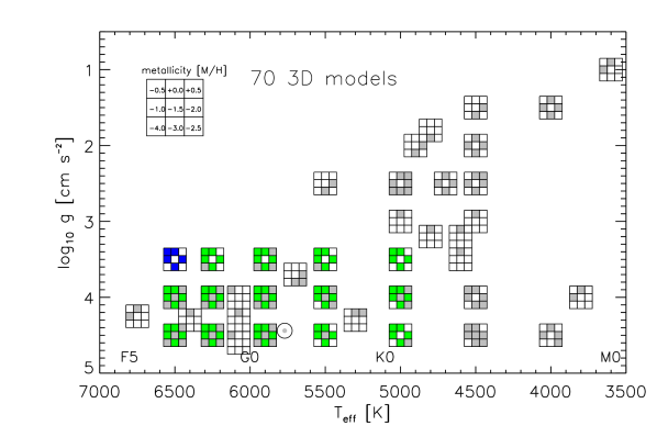
Figure 1: Overview of the grid of CO5BOLD 3D model atmospheres adopted for the computation of the fitting functions. The green filled squares mark the models that have been used in this work (five different metallicities, see legend at upper left), the grey squares indicate existing models that are part of the CIFIST grid but have not been considered in the present context. The blue squares highlight the missing models for which abundance corrections were derived by extrapolation (see Section 3.2). The solar 3D CO5BOLD model is indicated by the Sun symbol.

2 Stellar atmospheres and spectrum synthesis

2.1 3D CO5BOLD and 1D LHD model atmospheres

For this work, we adopted a sub-set of the CIFIST grid of 3D hydro-dynamical CO5BOLD model atmospheres (Ludwig et al., 2009) together with their corresponding 1D LHD models. These 1D models employ the same stellar parameters, micro-physics, chemical composition, and radiative transfer scheme as a CO5BOLD model, facilitating an unbiased 3D-1D differential comparison (Caffau et al., 2007). Our model grid is shown in Figure 1 in the $\log g-{T_{\rm eff}}$ plane that can be seen as a pseudo Hertzsprung-Russell (HR) diagram. The grid includes 70 3D models focusing on main-sequence and turn-off cool stars, represented by the following stellar parameters:

• ${T_{\rm eff}}$:       5000, 5500, 5900, 6300 and 6500 K,

• $\log g$:     3.5, 4.0 and 4.5 [cm s^-2],

• $\mathrm{[Fe/H]}$:  0.00, -0.5, -1.0, -2.0 and -3.0 dex.

The region around ${T_{\rm eff}}=6500$ K and $\log g=3.5$ (blue filled squares in Figure 1) is only scarcely populated in the (observed) H-R diagram, and for this reason models with such parameters are not available in the CIFIST grid. However, since a rectangular ${T_{\rm eff}}$–$\log g$ grid is more practical for defining a homogeneous fitting function, we decided to provide approximate results also for this missing combination of parameters by extrapolation of the lithium abundance corrections derived from the available atmospheres.

In Table A (see Appendix A), the main properties of the grid of selected models are listed. The effective temperature reported in the fourth column of Table A is the average ${T_{\rm eff}}$ over the sub-sample of $N_{\rm snap}$ selected snapshots (where $N_{\rm snap}$ is given in the third column) for each CO5BOLD simulation. Note that these ${T_{\rm eff}}$ deviate slightly from the nominal effective temperatures ${T_{\rm nom}}$ defining the rectangular grid depicted in Figure 1 (where ${T_{\rm nom}}=5000,\,5500,\,5900,\,6300$ and $6500$  K for all $\log g$ and $\mathrm{[Fe/H]}$). The fitting function will be developed on this fixed temperature grid after interpolation of the relevant quantities from the true ${T_{\rm eff}}$ to ${T_{\rm nom}}$.

For $\mathrm{[Fe/H]}$ = $0.0$ and $-2.0$, we have in addition computed independent, refined grids of 1D LHD models, covering the same range of gravities ($\log g$ = $3.5$, $4.0$, $4.5$) and effective temperatures ($5000\leq$${T_{\rm eff}}$ $\leq 6500$ K), but with a smaller and equidistant step of $\Delta$${T_{\rm eff}}$ = $100$ K. These auxiliary grids of 1D LHD models are useful for estimating the interpolation errors of the fitting functions developed in Section 4.

2.2 Library of 3D and 1D NLTE synthetic spectra

To ensure that our fitting functions cover a sufficiently wide range of lithium abundances, we consider eleven values of $A$(Li), from 1.0 to 3.0 with a step of 0.2 dex. For each abundance, we calculate individual NLTE departure coefficients for all snapshots of each 3D model and for their associated one-dimensional LHD counterparts, using our NLTE3D code (see, e.g., Steffen et al., 2015; Mott et al., 2017). We adopted the same lithium model atom as described in Mott et al. (2017), which is more complete than the one used by Sbordone et al. (2010), who, moreover, calculated the NLTE departure coefficients only for one representative value of $A\rm(Li)=2.2$ and assumed them to be valid for all considered lithium abundances in the range $0.9\leq$ $A$(Li) $\leq 3.3$.

Our approach of calculating a separate set of departure coefficients for each abundance constitutes a more reliable treatment of the NLTE effects over the full range of line strengths than the simplified approach adopted by Sbordone et al. (2010). In this sense, their fitting functions are superseded by the updated and extended version provided in the present work.

Once the NLTE departure coefficients are available, they are fed into the NLTE spectral synthesis code Linfor3D to compute a library of synthetic lithium line profiles. Our library consists of 770 3D NLTE lithium line profiles in the wavelength range $\lambda=[670.69-670.87]\,\rm nm$ ($14$ $\log g$–${T_{\rm eff}}$ combinations $\times 5$ metallicities $\times 11$ Li abundances) where each spectrum is the average over the selected snapshots. For each of these 3D NLTE spectra, we have computed corresponding 1D NLTE and 1D LTE spectra for comparison. In total, the library of synthetic spectra then comprises $3\times 770=2310$ spectra. In addition, we have computed a LTE curve-of growth (CoG) for each set of stellar parameters (${T_{\rm eff}}$, $\log g$, $\mathrm{[Fe/H]}$) which allows us to interpolate the 1D LTE equivalent width ($\rm EW_{1DLTE}$) of the lithium line over a wide range of $A$(Li) between $0.0$ and $4.5$ dex. In exactly the same way, we calculated a total of $1056$ additional 1D NLTE line profiles ($48$ $\log g$–${T_{\rm eff}}$ combinations $\times 2$ metallicities $\times 11$ Li abundances) plus the corresponding LTE CoGs from the auxiliary (refined) grids of 1D LHD models, available for $\mathrm{[Fe/H]}$ = $0.0$ and $-2.0$ only.

2.2.1 Microturbulence in 1D LHD models

In the 1D models, the small-scale velocity fields in the stellar photosphere is represented by the so-called microturbulence parameter $\xi_{\rm micro}$. As usual, $\xi_{\rm micro}$ describes a depth-independent isotropic Gaussian velocity distribution with a dispersion of $v_{\rm rms}=\,$$\xi_{\rm micro}$$/\sqrt{2}$.

In the 3D models, on the other hand, there is no need to introduce such artificial fudge parameter since the full velocity field is obtained naturally from the hydro-dynamical treatment of the convective motions in each CO5BOLD model atmosphere.

For a differential 3D-1D comparison, the microturbulence parameter of the 1D LHD model associated with a given 3D model should be adjusted such that the resulting small-scale velocity field matches (as closely as possible) the properties of the 3D hydrodynamical velocity field. Such a calibration has been presented by Dutra-Ferreira et al. (2016) who provide the following (theoretical) relation for $\xi_{\rm micro}$ as a function of effective temperature and surface gravity:

$$\xi_{\mathrm{micro}}=0.998+3.16\times 10^{-4}X-0.253Y-2.86\times 10^{-4}XY+0.165Y^{2},$$ (1)

where $X=T_{\rm eff}-5500$ [K] and $Y=\log g-4.0$.

This formula is the result of an analysis of 30 Fe i plus 7 Fe ii lines for which synthetic spectra have been computed adopting 3D CO5BOLD and 1D LHD model atmospheres of solar metallicity (we refer to this paper for more details). Equation (1) constitutes the most appropriate description of the $\xi_{\rm micro}$ parameter available in the context of 3D-1D comparisons. Even though formally valid for solar metallicity only, we use this relation to assign $\xi_{\rm micro}$ to all LHD models used in the present study. This may be justified by empirical evidence that $\xi_{\rm micro}$ depends only weakly on $\mathrm{[Fe/H]}$ (Sitnova et al., 2015; Mashonkina et al., 2017). The last column of Table A lists the values of $\xi_{\rm micro}$ computed with Eq. (1).

2.2.2 Line list

The lithium resonance doublet at $\lambda$670.8 nm is represented by 12 hyper-fine structure components, six for each isotope, extracted from the original list of Kurucz (1995), as explained in Mott et al. (2017). For the spectrum synthesis we assume a solar system isotopic ratio of $\mathrm{{}^{6}Li/^{7}Li}$=8.2% (e.g., Lodders, 2003).

Although our grid includes models with solar metallicity for which contributions to the equivalent width coming from some blend lines of different elements may be present, we excluded such features in the spectral synthesis, maintaining our focus on targets where these other atomic and molecular species have a negligible effect on the equivalent width (hereafter EW) of the lithium resonance doublet. See, however, Sect 6.3, where we discuss the applicability of our abundance corrections in the presence of blend lines.

Once the grids of 3D NLTE theoretical spectra and 1D (both NLTE and LTE) CoGs for the $\lambda$670.8 nm lithium line have been completed, we initiated the procedure for deriving the abundance corrections for each model as a function of $A$(Li) and their transformation into the functional fits. These are the result of several steps that are described in the next sections.

3 3D NLTE and 1D NLTE lithium abundance corrections

3.1 Definition

When dealing with the concept of abundance corrections, it is important to define properly how such corrections are derived since they can be calculated in multiple ways. Considering the 1D NLTE case, the corrections, $\Delta_{\rm 1DNLTE-1DLTE}$, are usually defined as a function of the 1D LTE abundance, $A\rm(Li)_{1DLTE}$, such that:

$$A\mathrm{(Li)_{1DNLTE}}=A\mathrm{(Li)_{1DLTE}}+\Delta_{\rm 1DNLTE-1DLTE}\,.$$ (2)

To derive this correction for a given $A\rm(Li)_{1DLTE}$ (which is usually the result of a standard 1D LTE analysis), one first has to compute the 1D LTE equivalent width associated with this LTE lithium abundance, EW_1DLTE. The next step is the search for the 1D NLTE lithium abundance, $A\rm(Li)_{1DNLTE}$ that provides the same EW_1DLTE value. Note that this step requires the computation of a 1D NLTE curve-of-growth. The sought 1D NLTE abundance correction ($\Delta_{\rm 1DNLTE-1DLTE}$) is then defined as the difference of the two abundances. These corrections can be applied to standard 1D LTE abundances to correct them for non-LTE effects.

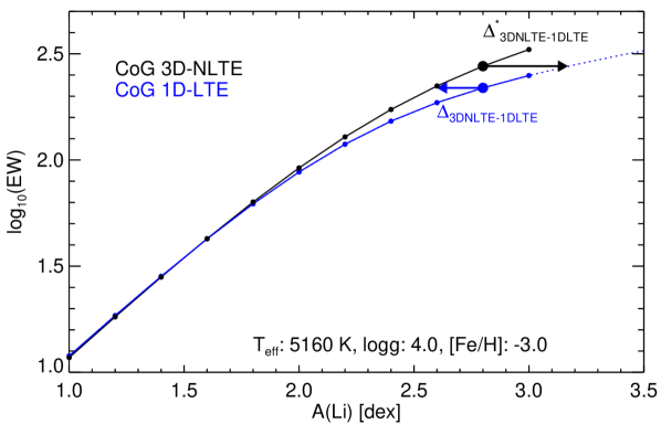
Figure 2: Two different definitions of abundance corrections for the example of a strong Li line on the non-linear part of the CoG. The correction $\Delta^{\ast}_{\rm 3DNLTE-1DLTE}$ is indicated by the black horizontal arrow starting on the 3D NLTE CoG (black) at $A$(Li) = $2.8$ and ending at a higher abundance given by the intersection with the 1D LTE CoG (blue). Conversely, the correction $\Delta_{\rm 3DNLTE-1DLTE}$ is given by the blue horizontal arrow starting on the 1D LTE CoG (blue) at the same abundance $A$(Li) = $2.8$ and extending to the 3D NLTE CoG (black).

A completely analogous procedure could be applied to derive the 3D NLTE corrections $\Delta_{\rm 3DNLTE-1DLTE}$, again as a function of the 1D LTE abundance $A\rm(Li)_{1DLTE}$, allowing to correct the 1D LTE abundance for the combined 3D plus NLTE effect:

$$A\mathrm{(Li)_{3DNLTE}}=A\mathrm{(Li)_{1DLTE}}+\Delta_{\rm 3DNLTE-1DLTE}\,.$$ (3)

The “inverse” abundance correction $\Delta^{\ast}_{\rm 3DNLTE-1DLTE}$ is defined as the correction that has to be added to a given 3D NLTE abundance in order to obtain the corresponding 1D LTE abundance. It has the opposite sign but in general (for partly saturated lines) a different magnitude than the commonly used “forward” correction $\Delta_{\rm 3DNLTE-1DLTE}$. While it is technically more straightforward to derive the “inverse” corrections $\Delta^{\ast}_{\rm 3DNLTE-1DLTE}$ from the theoretical models, they are of less practical interest and we calculate them only as an intermediate step. Eventually, we provide the “forward” corrections $\Delta_{\rm 3DNLTE-1DLTE}$ as a function of the 1D LTE lithium abundance that is typically derived by analyzing an observed stellar spectrum.

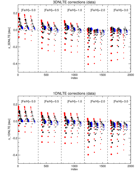
Figure 3: Overview of the Li abundance corrections $\Delta_{\rm 3DNLTE-1DLTE}$ (top) and $\Delta_{\rm 1DNLTE-1DLTE}$ (bottom) as evaluated on the complete 4D parameter grid. For each metallicity, a total of $165$ points indicates the corrections as a function of an arbitrary spectrum number that runs over $A$(Li), ${T_{\rm eff}}$, and $\log g$. Large (left group), intermediate (middle group), and small dots (right group) correspond to $\log g$ = $3.5$, $4.0$, and $4.5$, respectively. For each gravity, ${T_{\rm eff}}$ increases from left to right ($5000$ K: red, $5500$ K: black, $5900$ K: gray, $6300$ K: black, $6500$ K: blue). Each effective temperature is represented by $11$ dots indicating the results for $1.0\leq A$(Li) $\leq 3.0$.

3.2 Computation of the lithium abundance corrections

The abundance corrections defined in Section 3.1 are derived by the following procedure.

Given our fixed set of lithium abundances ($1.0\leq A\rm(Li)\leq 3.0$), we compute the equivalent width of the Li i doublet from the 3D models in full 3D NLTE (EW_3DNLTE), and the LTE and NLTE EWs from the associated 1D LHD models (EW_1DLTE and EW_1DNLTE, respectively) by numerical integration of the synthetic lithium line profiles over the wavelength range $\Delta\lambda$ = $[670.69-670.87]$ nm. These data define three different curves-of-growth for each set of stellar parameters, corresponding to 3D NLTE, 1D LTE, and 1D NLTE treatment, respectively.

As an illustration, we show in Figure 2 the 3D NLTE CoG (black) and the 1D LTE CoG (blue) for the models with ${T_{\rm eff}}$ = $5160$ K, $\log g$ = $4.0$ and $\mathrm{[Fe/H]}$ = $-3.0$. Filled dots mark the computed EWs at the prescribed grid of lithium abundances, continuous lines show the CoGs obtained by piecewise cubic interpolation. According to the above definition, the 3D NLTE abundance correction $\Delta_{\rm 3DNLTE-1DLTE}$ corresponds to the horizontal distance between the two CoGs. For a given 1D LTE abundance (e.g., $A\rm(Li)=2.8$), $\Delta_{\rm 3DNLTE-1DLTE}$ is negative and its magnitude is indicated by the length of the blue horizontal arrow, which can be easily obtained by interpolation.

For completeness, Figure 2 also shows the “inverse” abundance correction $\Delta^{\ast}_{\rm 3DNLTE-1DLTE}$, indicated by the black horizontal arrow. This is the correction that has to be applied to a given 3D NLTE abundance in order to obtain the corresponding 1D LTE abundance. As mentioned above, it is not considered here as it is not of practical interest.

We derived the 1D NLTE corrections $\Delta_{\rm 1DNLTE-1DLTE}$ following the same method, replacing the $\rm EW_{3DNLTE}$ by the 1D NLTE equivalent widths $\rm EW_{1DNLTE}$, computed with the microturbulence parameter that is listed in Table A for each model atmosphere. The obtained grids of 3D NLTE and 1D NLTE abundance corrections have four dimensions: ${T_{\rm eff}}$, $\log g$, $\mathrm{[Fe/H]}$, $A$(Li). At this stage, however, the grids need some further manipulation, before we are able to represent them by analytical expressions.

The first issue is that the corrections are based on equivalent widths that are computed for the real effective temperatures that depart slightly from the fixed nominal temperature grid ${T_{\rm nom}}$ = $5000,5500,5900,6300$, and $6500$ K. This means that the temperature grid is slightly different for each ($\log g$, $\mathrm{[Fe/H]}$) combination, preventing a straightforward comparison of abundance corrections for models with different surface gravity or metallicity at fixed ${T_{\rm eff}}$. This difficulty is eliminated by interpolating the corrections from the actual ${T_{\rm eff}}$ grid to the fixed ${T_{\rm nom}}$ grid, separately for each ($\log g$, $\mathrm{[Fe/H]}$) combination and for each of the 11 values of $A$(Li). Here we employ again a piecewise cubic interpolation, in some cases involving some very slight (uncritical) extrapolation. After this step, the grids of 3D NLTE and 1D NLTE abundance corrections are represented on a four-dimensional rectangular grid.

The second issue concerns the missing corrections for surface gravity $\log g$ = $3.5$ and ${T_{\rm eff}}$ = $6500$ K. Due to the lack of the corresponding model atmospheres in the CIFIST grid (blue squares in Figure 1), we decided to find these values by means of extrapolation from the available corrections. For given $\mathrm{[Fe/H]}$ and $A$(Li), we compute the missing corrections as the average of the results obtained from two orthogonal linear extrapolations: (i) using the available corrections at fixed $\log g$=3.5 and ${T_{\rm nom}}$=($5900,6300$) K, and (ii) using the corrections at fixed ${T_{\rm nom}}$=$6500$ K and $\log g$=($4.0,4.5$).

Even if we could have generated the missing 1D LHD models and the corresponding 1D LTE and NLTE spectra, we decided to compute the missing 1D NLTE corrections by extrapolation in exactly the same way as in the 3D case described above. Comparison with the independent results from the auxiliary (refined) grid of 1D LHD models for $\mathrm{[Fe/H]}$ = $0.0$ and $-2.0$ (see Sect. 2.1) reveals that the extrapolation works perfectly for $\log g$ = $4.5$, but may introduce an error of the order of $-0.01$ dex for $\log g$ = $3.5$ and $4.0$.

After these preparatory steps, our rectangular grids of $\Delta_{\rm 3DNLTE-1DLTE}$ and $\Delta_{\rm 1DNLTE-1DLTE}$ corrections are complete. An overview of the corrections as a function of the grid parameters $A$(Li), ${T_{\rm eff}}$, $\log g$, and $\mathrm{[Fe/H]}$ is presented in Figure 3. The dependence of the 3D and 1D corrections on the stellar parameters and the lithium abundance is qualitatively similar. For weak lines (low $A$(Li)), they are generally positive, while they tend to be negative for the highest Li abundance. The corrections are most sensitive to the line strength for the coolest models. They are most negative for the lowest metallicities, reaching values of at least $-0.3$ dex at $\mathrm{[Fe/H]}$ $\leq$ $-2.0$, ${T_{\rm eff}}$ = $5000$ K, $A$(Li) = $3.0$.

4 Analytical approximations

4.1 Lithium abundance corrections

In the following, we derive a first parametric equation (hereafter FFI_3DNLTE, FFI_1DNLTE) that approximates the $\Delta_{\rm 3DNLTE-1DLTE}$ and $\Delta_{\rm 1DNLTE-1DLTE}$ corrections, respectively, as a function of ${T_{\rm eff}}$, $\log g$, $\mathrm{[Fe/H]}$, and $A$(Li).

An effective way to achieve this is to perform, as a first step, a 2D-fit of the corrections in the ${T_{\rm nom}}$-$A$(Li) plane for each $\mathrm{[Fe/H]}$ and $\log g$, separately. For this purpose, we utilized the IDL procedure SFIT which allows to perform a surface fit to a set of 2-dimensional data (in our case the $\Delta$ values given on a rectangular grid as a function of ${T_{\rm nom}}$ and $A$(Li)). SFIT returns an array of coefficients, the number of which depends on the chosen degree of the polynomial function used in the fitting.

Obviously, the goal is to achieve a reasonable fit of the corrections with a relatively low number of coefficients. After several tests we found that our corrections were satisfactorily fitted by a polynomial function with a maximum degree equal to 4, expressed as:

$$\Delta(y,z)=\sum_{j=0}^{4}y^{j}\sum_{k=0}^{4-j}z^{k}\cdot c_{jk}\,,$$ (4)

where $y=A\mathrm{(Li)}_{\rm 1DLTE}$ ($1.0\leq y\leq 3.0$) and $z=(T_{\rm nom}/1000-5)$ ($0\leq z\leq 1.5$). Such normalized coordinates make the 15 coefficients $c_{jk}$ dimensionless and of similar magnitude.

Lowering the degree of the polynomial function, we noticed a significant degradation of the fitting quality for some metallicities or for some surface gravities. As a consequence, we conclude that in order to fit homogeneously the whole set of corrections with a unique polynomial form, the optimal choice is a maximum degree equal to 4.

Figure 4: Contour plots of the 3D NLTE abundance corrections in the ${T_{\rm eff}}$–$A$(Li)_1DLTE plane. Each panel shows the corrections computed with FFI_3DNLTE (Eq. 6) for all combinations of surface gravity and metallicity as given in the title of each plot.

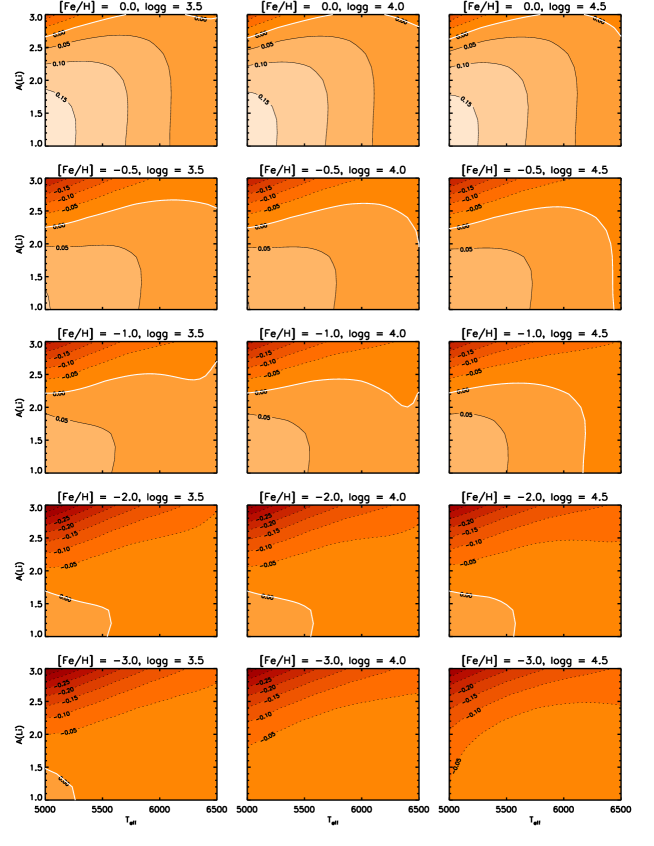
Figure 5: Contour plots of the 1D NLTE abundance corrections in the ${T_{\rm eff}}$–$A$(Li)_1DLTE plane. Each panel shows the corrections computed with FFI_1DNLTE (Eq. 6) for all combinations of surface gravity and metallicity as given in the title of each plot.

Following this strategy, we obtain a set of 15 numerical coefficients for each given metallicity $\mathrm{[Fe/H]}$ and gravity $\log g$ that defines the fitting surface of the corrections in the ${T_{\rm nom}}$-$A$(Li) plane.

Noticing that the gravity dependence of the corrections is rather weak, we represent the gravity dependence of the coefficients $c_{jk}$ by a linear function in the normalized surface gravity $x=\log g-3.5$ ($0\leq x\leq 1$) as:

$$c_{jk}(x)=\sum_{i=0}^{1}x^{i}\cdot c_{ijk}\,.$$ (5)

The coefficients $c_{ijk}$ are obtained from the $c_{jk}$ given at the three gravities ($x=0.0,\,0.5,\,1.0$) by standard linear regression, separately for each metallicity $\mathrm{[Fe/H]}$.

For each particular metallicity value of our grid, we thus obtain the following final fitting function that describes the $165$ NLTE lithium abundance corrections as a function of ${T_{\rm eff}}$, $\log g$, and $A$(Li) through 30 numerical coefficients:

$$\texttt{\rm FFI}=\Delta\left({T_{\rm eff}},\log g,A\mathrm{(Li)}\right)=\sum_{i=0}^{1}x^{i}\sum_{j=0}^{4}y^{j}\sum_{k=0}^{4-j}z^{k}\cdot c_{ijk},$$ (6)

The list of 30 coefficients $c_{ijk}$ are given, for each metallicity covered by our grid ($\mathrm{[Fe/H]}=0.0,-0.5,-1.0,-2.0$ and $-$3.0 dex), in Tables 3 ($\Delta_{\rm 3DNLTE-1DLTE}$) and 4 ($\Delta_{\rm 1DNLTE-1DLTE}$) in Appendix B.

We decided not to include the metallicity as a fourth parameter of our fitting function since the trend of the corrections as a function of $\mathrm{[Fe/H]}$ is not as simple as for the $\log g$ dependence. Finding a global fitting function able to fit our data for each combination of ${T_{\rm eff}}$, $\log g$, $\mathrm{[Fe/H]}$, and $A$(Li) simultaneously would have required the inclusion of an impractical number of coefficients.

When applying this fitting function to metallicities other than those that are tabulated, a further interpolation of the obtained $\Delta$ values to the desired $\mathrm{[Fe/H]}$ is necessary. We do not expect that this final operation would compromise the precision of the derived abundance corrections.

To facilitate the practical application of the analytical fitting function, we provide a Python script that computes the corrections as a function of the four parameters ${T_{\rm eff}}$, $\log g$, $\mathrm{[Fe/H]}$, and $A$(Li), using the coefficients listed in Tables 3 and 4, respectively, according to Eq. (6), and subsequently performing a piecewise cubic monotonic interpolation (see Steffen, 1990) in $\mathrm{[Fe/H]}$. An overview of the lithium abundance corrections obtained with the fitting functions FFI_3DNLTE and FFI_1DNLTE is shown in Figures 4 and 5, respectively, as a series of contour plots in the ${T_{\rm eff}}$ – $A$(Li) plane, separately for each combination of $\mathrm{[Fe/H]}$ and $\log g$.

To check how well our fitting functions are able to represent the $\Delta_{\rm 3DNLTE-1DLTE}$ and $\Delta_{\rm 1DNLTE-1DLTE}$ input data, we computed for each combination of $\mathrm{[Fe/H]}$, $\log g$, ${T_{\rm eff}}$, and $A$(Li) the difference between the abundance correction predicted by the fitting function and the value of the original input data. Figure 17 shows these differences at the 4D grid points, both for the 3D NLTE and the 1D NLTE corrections.

For solar metallicity, the residuals $\delta_{\rm FFI}$ fall in the range $|\delta_{\rm FFI}|\la 0.01$, with a rms mean of $\langle\delta^{2}_{\rm FFI}\rangle^{1/2}<0.004$. For all subsolar metallicities, the residuals are slightly larger, lying in the range $|\delta_{\rm FFI}|\la 0.02$, with a typical rms mean of $0.005$. With very few exceptions, the maximum residuals occur at ${T_{\rm eff}}$ = $5000$ K for the extreme lithium abundances, $A$(Li) = $1.0$ or $3.0$.

In the 1D case, we can additionally evaluate the interpolation errors of FFI_1DNLTE for $\mathrm{[Fe/H]}$ = $0.0$ and $-2.0$ by comparison with the corrections derived independently from the auxiliary grid of 1D LHD models for a refined sample of effective temperatures. We find that the interpolation errors at the intermediate temperatures have about the same amplitude as the fitting function errors at the nodes of the original grid, with $|\delta_{\rm FFI}|\la 0.016$ dex in all cases, as shown in full detail in Fig. 18. At an arbitrary point in the multidimensional parameter space (${T_{\rm eff}}$, $\log g$, $A$(Li)), the interpolation error may be somewhat larger, due to the additional (unknown) interpolation errors in $\log g$ and $A$(Li). However, we can assume that the latter two interpolation errors are small compared to the interpolation error in ${T_{\rm eff}}$, due to the weak gravity dependence of the corrections and the fine spacing of the original $A$(Li) grid, respectively, such that the interpolation errors shown in Fig. 18 can still be considered as a valid order-of-magnitude estimate of the total interpolation error.

Taken together, the error analysis indicates an overall good fit of tabulated abundance corrections by our fitting function FFI_1DNLTE, and by implication FFI_3DNLTE, across the whole ${T_{\rm eff}}$–$\log g$–$A$(Li) space. As an additional benefit, the fitting functions smooth out small numerical artifacts in the raw data.

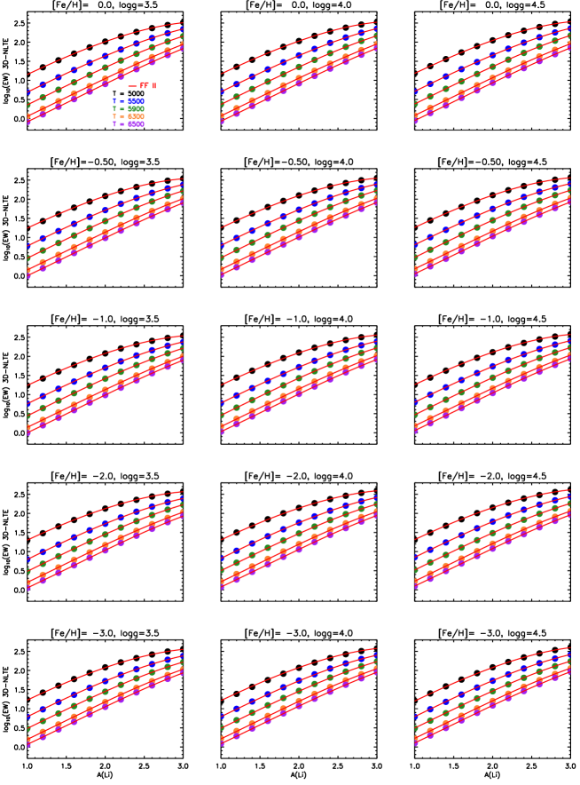
Figure 6: Comparison between the input data (filled dots, color-coded according to effective temperatures as shown in the legend of the upper left panel) and the resulting fitting polynomial FFII_3DNLTE (Eq. 7, red continuous line). The surface gravity and the metallicity values are shown in the title of each plot.

4.2 From $A$(Li) to EW

In this section we describe the derivation of a second parametric equation (hereafter FFII_3DNLTE, FFII_1DNLTE) which allows the computation of the 3D NLTE and 1D NLTE equivalent width values for the input parameters ${T_{\rm eff}}$, $\log g$, $\mathrm{[Fe/H]}$, and lithium abundance $A$(Li).

The principal ingredient is obviously represented by the equivalent width values of the lithium doublet for each one of the 70 model atmospheres in our grid as computed for each one of the 11 lithium abundances in the range $A\rm(Li)=[1.0\,..\,3.0]$. For the 1D case only, the microturbulence parameter $\xi_{\rm micro}$ of each model has been set to the value calculated by means of Eq. (1). Otherwise, the derivation of the functional fit described in the following is the same for the 3D NLTE and the 1D NLTE case.

In a first step, the EWs obtained from the model atmospheres (at given $\log g$, $\mathrm{[Fe/H]}$, and $A$(Li)) were interpolated from the actual ${T_{\rm eff}}$ values to the fixed ${T_{\rm nom}}$ grid. In a second step, the resulting rectangular grid of EW values is completed by estimating the missing EW values at ${T_{\rm nom}}=6500$ K and $\log g=3.5$ for each metallicity by means of linear extrapolation as described in Section 3.2.

For each $\log g$ – $\mathrm{[Fe/H]}$ combination, we thus obtain a complete, rectangular grid of EW values as a function of temperature and lithium abundance. The derivation of the fitting function FFII is completely analogous to the procedure to derive the fitting function FFI for the abundance corrections as described in Sect. 4.1. First we use the IDL procedure SFIT to compute the coefficients of the two-dimensional polynomial function of maximum degree four providing the best surface fit to the (logarithmic) EWs in the $y$ – $z$ plane, separately for each of the $15$ $\log g$ – $\mathrm{[Fe/H]}$ sets. Then the $\log g$-dependence of the coefficients is represented by a linear function in $x=\log g-3.5$. In this way, we obtain for each of the five metallicities a set of $30$ dimensionless coefficients $w_{ijk}$ that define the fitting function FFII for the EWs. It has the same form as Eq. (6):

FFII $$= \log_{10}(\mathrm{EW})\left({T_{\rm eff}},\log g,A\mathrm{(Li)}\right)$$ (7)

$$= \sum_{i=0}^{1}x^{i}\sum_{j=0}^{4}y^{j}\sum_{k=0}^{4-j}z^{k}\cdot w_{ijk}\,,$$

where EW is the equivalent width in mÅ, and as before $x$ = $\log g-3.5$, $y$ = $A\mathrm{(Li)}$, $z$ = ($T_{\rm nom}/1000-5$). The coefficients $w_{ijk}$ are given in Tables 5 and 6 for the 3D NLTE and 1D NLTE case, respectively.

The comparison plot shown in Fig. 6 demonstrates how well our function fits the 3D NLTE input data. Clearly, the FFII fitting polynomial of maximum degree four (continuous red lines) ensures a very good agreement between the input EW (filled dots, color coded according to ${T_{\rm nom}}$) across the full parameter space covered by our grid. The fit of the 1D NLTE EWs is even slightly better. For both 3D and 1D, the relative fitting function error is $|\Delta$EW/EW— $\la$ $2$ % with few exceptions, while the rms mean fitting error on the 4D parameter grid is less than $1$ %. The maximum global fitting function error is $\Delta$EW/EW = $+3.9$ % for FFII_3DNLTE ($\mathrm{[Fe/H]}$ = $-3.0$, $\log g$ = $4.0$, ${T_{\rm eff}}$ = $5000$ K, $A$(Li)=$1.0$) and $-3.4$ % for FFII_1DNLTE ($\mathrm{[Fe/H]}$ = $-1.0$, $\log g$ = $4.0$, ${T_{\rm eff}}$ = $5900$ K, $A$(Li)=$1.0$). Interpolation errors are of similar size. For further details see Figs. 19 and 20.

For practical application of FFII, we provide a Python script that computes the EWs as a function of the four parameters ${T_{\rm eff}}$, $\log g$, $\mathrm{[Fe/H]}$, and $A$(Li), using the coefficients listed in Tables 5 and 6, respectively, according to Eq. (7), followed by a piecewise cubic monotonic interpolation in $\mathrm{[Fe/H]}$.

4.3 From EW to $A$(Li)

With the equivalent width fitting functions FFII presented in Section 4.2 and defined by Eq. 7, it is in principle already possible to derive the 3D NLTE and 1D NLTE lithium abundances corresponding to a given input equivalent width by numerical inversion. Using the provided FFII procedure, one could construct a curve-of-growth for an appropriate range of abundances that maps to a range of equivalent widths covering the “observed” EW. The desired lithium abundance, $A\rm(Li)_{3DNLTE}$ or $A\rm(Li)_{1DNLTE}$, for that particular EW may then be easily derived through interpolation in the inverted curve-of-growth EW$\,\rightarrow\,A$(Li).

As an alternative to this numerical procedure, we have developed a third parametric fitting formula (hereafter FFIII) that represents the inverse of FFII. As such, it provides the 3D NLTE or 1D NLTE value of $A$(Li) for a given input EW and stellar parameters ${T_{\rm eff}}$, $\log g$, and $\mathrm{[Fe/H]}$. As an algebraic inversion of FFII is not feasible, we construct the inverse fitting function FFIII from scratch, based on the raw data (EW as a function of $A$(Li)).

The EW grid we start with has already been interpolated to the nominal temperature scale ${T_{\rm nom}}$ and completed by extrapolation where data are missing, as described in Section 4.2. In principle this grid would be ready for the fitting, but in this case we encounter the additional difficulty that the data in the ${T_{\rm nom}}$ – EW plane are not given on a rectangular grid, as shown in Fig, 7 (upper panel) for the 3D case $\log g$ = $3.5$, $\mathrm{[Fe/H]}$ = $0.0$. While fitting data on an irregular grid is not impossible, it becomes easier if the parameter space is rectangular. Then it is possible to use the standard procedures to obtain a good fit of the data with a polynomial function of relatively low degree. However, it is not feasible to simply remap the data points to such a rectangular grid, as this would require an unacceptable amount of extrapolation. We also note that, from a physical point of view, a rectangular ${T_{\rm nom}}$ – EW grid is not adapted to the systematic temperature dependence of the line strength (see Fig, 7a).

In view of theses difficulties, we introduce the concept of a “scaled equivalent width” $w$. As a first step, we define two auxiliary fitting curves indicated in the lower panel of Figure 7 as $p(z)$ and $q(z)$. These two quadratic curves approximate the EW values as a function of $z=({T_{\rm nom}}/1000-5)$ for the extreme abundances of our grid, $A\rm(Li)=1.0$ ($p$, blue curve) and $A\rm(Li)=3.0$ ($q$, red curve), respectively. The scaled equivalent width is then defined by the following temperature-dependent conversion:

$$w(z)=\frac{\log_{10}(\mathrm{EW})-p(z)}{q(z)-p(z)},$$ (8)

where $p(z)=p_{0}+p_{1}z+p_{2}z^{2}$ and $q(z)=q_{0}+q_{1}z+q_{2}z^{2}$ are the aforementioned boundary fitting curves. We note that the quality of linear fits was found to be unsatisfactory.

In principle, the coefficients $p_{m},q_{n}$ depend on both $\log g$ and $\mathrm{[Fe/H]}$. However, the fact that the EW values are only very weakly dependent on surface gravity allows us to consider two “global” parabolas to scale all the equivalent width values for a given metallicity. The coefficients $p_{m}(\mathrm{[Fe/H]})$ and $q_{n}(\mathrm{[Fe/H]})$ were obtained by averaging the respective individual coefficients for the three surface gravities. This approximation has the advantage of decreasing the number of numerical coefficients defining our inverse fitting function FFIII. The averaged coefficients are provided in Table 7 of Appendix B as a function of $\mathrm{[Fe/H]}$ for both the 3D NLTE and the 1D NLTE case.

The EW scaling largely removes the systematic trend with ${T_{\rm eff}}$, as shown in the lower panel of Figure 7, where we now plot the distribution of the data points in the $z-w$ plane. By construction, $0\leq w\leq 1$, but the grid is still not perfectly rectangular. However, a rectangular grid can be easily created now by interpolation, without the need for any extrapolation.

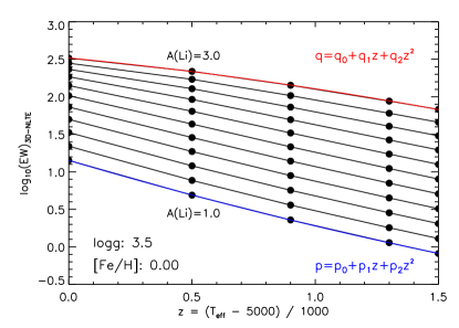
Figure 7: Distribution of the 3D NLTE data points for $\log g$ = $3.5$, $\mathrm{[Fe/H]}$ = $0.0$ in the ${T_{\rm eff}}$ – EW plane (upper panel), and in the ${T_{\rm eff}}$ – $w$ plane (lower panel) where the systematic trend with temperature is eliminated by normalizing the EWs with the help of the parabolic boundary curves $p(z)$ and $q(z)$ shown in the upper panel (see text for details).

For this purpose, we selected 21 equidistant values between $w=0$ and $1$ with a step of $\Delta w=0.05$ that will constitute, together with the temperature scale $z$, the rectangular parameter space on which our lithium abundances are distributed. The 21 $A$(Li) values that correspond to the fixed $w$ grid are found by piecewise cubic, monotonic interpolation, separately for each $z$, $\log g$, and $\mathrm{[Fe/H]}$.

A this point the rectangular grid of lithium abundances can be fitted in the rectangular $z-w$ parameter space. Also in this case, we choose to fit the surface of the abundance values by a two-dimensional polynomial function of maximum degree 4, following exactly the same method as for the abundance corrections (FFI, Section 4.1) and the equivalent widths (FFII, Section 4.2), again assuming a linear gravity dependence of the coefficients.

The final analytic expression can be written as:

FFIII $$= A\mathrm{(Li)}\left({T_{\rm eff}},\log g,\mathrm{EW}\right)$$ (9)

$$= \sum_{i=0}^{1}x^{i}\sum_{j=0}^{4}w^{j}\sum_{k=0}^{4-j}z^{k}\cdot a_{ijk}\,,$$

with $w$ = $(\log_{10}$(EW)$-p(z))/({q(z)-p(z))}$, $p(z)=p_{0}+p_{1}z+p_{2}z^{2}$, $q(z)=q_{0}+q_{1}z+q_{2}z^{2}$, and $x$ = $\log g$ $-3.5$, $z=({T_{\rm nom}}/1000-5)$.

The coefficients $a_{ijk}$ are presented as a function of $\mathrm{[Fe/H]}$ in Appendix B, in Tables 8 and 9 for the 3D NLTE and the 1D NLTE case, respectively, while the coefficients $p_{m}$ and $q_{n}$ describing the transformation from EW to $w$ are provided in Table 7.

Employing Eq. (9), optionally using the provided Python script that in addition performs interpolation in $\mathrm{[Fe/H]}$, the user obtains directly the 3D NLTE or the 1D NLTE lithium abundance for given stellar parameters and the measured EW, avoiding intermediate steps such as the aforementioned inversion that is required if one uses the forward fitting function FFII for this purpose.

We have checked that our inverse fitting function FFIII works very well. The fitting function error is evaluated by taking the equivalent widths EW(${T_{\rm eff}}$, $\log g$, $\mathrm{[Fe/H]}$, $A$(Li)) on the grid points of our full 4D parameter space as input and comparing the output of FFIII, $A$(Li)_FFIII, with the true (input) lithium abundance $A$(Li)_inp. As shown in Fig. 21, we find a maximum fitting function error of $A$(Li)${}_{\rm FFIII}-A$(Li)${}_{\rm inp}=-0.033$ dex, both for FFII_3DNLTE and FFII_1DNLTE, occurring at $\mathrm{[Fe/H]}$=$-0.5$, $\log g$=$4.0$, ${T_{\rm eff}}$=$5000$ K, $A$(Li)=$3.0$, where the equivalent with of the lithium doublet is $\ga 360$ mÅ. Apart from these extreme conditions, FFIII performs much better, with a rms mean fitting error of $\approx 0.006$ dex in both cases. The interpolation error is typically confined in the range $|\delta_{\rm FFIII}|\la 0.02$ (see Fig. 22).

5 Comparison with other authors

In this section, we compare the results of our fitting functions with some of the existing work in the literature that is focused on lithium abundance corrections and parametric equations for deriving NLTE lithium abundances from EW measurements. The availability of such independent analysis performed on a common range of stellar parameters is used to check the consistency of our results and to discuss potential differences in the adopted methods.

5.1 $A$(Li) to EW: comparison with Sbordone et al. (2010)

The work presented in the previous sections has some important features in common with the work published by Sbordone et al. (2010). Both investigations are based on 3D CO5BOLD model atmospheres and the related 1D LHD models, and use the same codes to compute the NLTE departure coefficients (NLTE3D) and the line formation of the lithium doublet (Linfor3D). The immediate advantage of this comparison is that systematic differences in the results due to different input model atmospheres can be excluded.

In Figures 8 and 9, we show a comparison of the results, in terms of CoGs obtained by applying both Sbordone et al. (2010)’s fitting function in the form EW(${T_{\rm eff}}$,$\log g$,$\mathrm{[Fe/H]}$,$A$(Li)) and our FFII(${T_{\rm eff}}$, $\log g$, $A$(Li); $\mathrm{[Fe/H]}$) (Eq. 7) to the lithium abundance range $A\rm(Li)=[1.0,3.3]$. Although our functions are valid over a wider range of metallicity, we limit the comparison to the stellar parameters that both works have in common, namely ${T_{\rm eff}}$ = $5500,5900,6300,6500$ K, $\log g$ = $3.5,4.0,4.5$ and $\mathrm{[Fe/H]}$ = $-2.0$ (Figure 8) and $-3.0$ (Figure 9).

It is worth noting that the lithium abundance range, specifically the upper boundary below which the function of Sbordone et al. is applicable, depends on the stellar parameters. This is shown in Figures 8 and 9 by means of colored vertical dashed lines. Beyond these upper limits, their equation is not trustworthy, since it operates in complete extrapolation. On the other hand, our fitting function FFII is valid across the whole abundance range from $A$(Li) = $[1.0$ to $3.0]$, independently of the stellar parameters.

If we consider the abundance range where both fitting functions are well defined, we can conclude that the results are in a very good agreement. Only very subtle differences in the derived CoGs can be appreciated towards hotter models and at larger lithium abundances. This could be related to the different lithium model atom or to the choice of Sbordone et al. (2010) of using a single set of NLTE departure coefficients, computed for each model atmosphere assuming $A\rm(Li)=2.2$. This approximation can only be considered reasonable as long as the lithium line is rather weak. In the case of a stronger lithium line (larger $A$(Li)), the NLTE departure coefficients are no longer independent of the lithium abundance, thus introducing additional non-linearities in the partly saturated region of the curve-of-growth. In the present work, we therefore compute consistent departure coefficients for each individual $A$(Li).

We have verified that, on average, the departure coefficients tend to be driven closer to unity (i.e., the level populations are driven towards LTE) as the lines become optically thick. This implies that the Sbordone at al. approximation produces synthetic lithium lines that tend to be too weak for $A$(Li) $>$ $2.2$. In case of the 3D model with ${T_{\rm eff}}$ = $5500$ K, $\log g$ = $4.0$, $\mathrm{[Fe/H]}$ = $-2.0$, and $A$(Li)  $=3.0$, for instance, we find EW = $226$ mÅ when using the departure coefficients computed for $A$(Li) = $2.20$, and EW = $263$ mÅ when using the consistent departure coefficients computed for $A$(Li) = $3.00$, thus $\Delta\log(\mathrm{EW})$ $\approx$ $0.07$ dex. While going in the right direction, this effect is too small to explain the discrepancies of the order of $0.3$ dex seen in Fig. 8 at $A$(Li)  $=3.0$.

We conclude that these large differences are mainly due to extrapolation errors arising when the Sbordone et al. (2010) formula is applied outside its range of validity. Such errors can now be avoided by using the extended fitting function FFII which correctly tracks the impact of NLTE effects across the abundance grid for each given model atmosphere. If $A$(Li) falls in the range where both approximations are valid, FFII and Sbordone et al. (2010) are in very close agreement, as expected. Since the “inverse” fitting function of Sbordone et al., EW to $A$(Li), is the algebraic inversion of their “forward” fitting function, a comparison with our FFIII would not allow for any further conclusions.

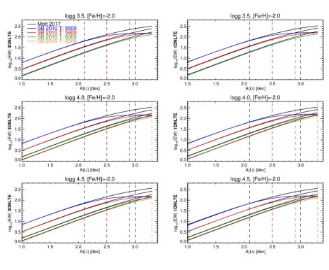
Figure 8: Comparison between the Li 670.8 nm curves-of-growth computed with the fitting function of Sbordone et al. (2010) for $\mathrm{[Fe/H]}$ = $-2.0$ (colored continuous lines) and with our function FFII (black solid lines) for the 3D NLTE (left) and 1D NLTE (right) cases, respectively, and for three values of surface gravity ($\log g$ = $3.5$, $4.0$, and $4.5$). The vertical colored dashed lines indicate the upper limits of the lithium abundance range for which the relation of Sbordone et al. (2010) is well defined (beyond these limits the fitting function is evaluated in extrapolation). Different colors denote the different effective temperatures at which the relations are evaluated (see legend in upper left panel). The black dashed line represents the upper abundance limit up to which our fitting function is defined ($A$(Li) = $3.0$ for all temperatures).

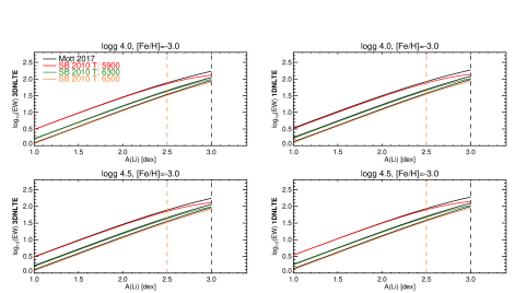
Figure 9: Same as Figure 8 but for $\mathrm{[Fe/H]}$ = $-3.0$, $\log g$ = $4.0$ and $4.5$. In this case, the upper limits to which the fitting function by Sbordone et al. (2010) is safely applicable coincides with $A\rm(Li)=2.5$ for all temperatures (vertical dashed orange line). Our fitting function is valid up to $A$(Li) = $3.0$ (vertical dashed black line).

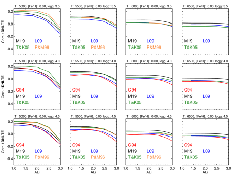
Figure 10: Comparison between the results of our fitting function FFI for the 1D NLTE lithium abundance corrections and those published by other authors for $\mathrm{[Fe/H]}$ = $0.0$, $\log g$ = $3.5,4.0,$ and $4.5$, ${T_{\rm eff}}$ = $5000,5500,6000,$ and $6500$ K. The black lines labeled as M19 show our results, whereas the colored lines show the corrections of other authors: C94 (Carlsson et al., 1994, red), P&M96 (Pavlenko & Magazzu, 1996, orange), T&K05 (Takeda & Kawanomoto, 2005, green), and L09 (Lind et al., 2009, blue).

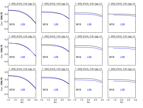
Figure 11: Same as Figure 10 but for $\mathrm{[Fe/H]}=-0.5$. For this metallicity, a comparison is only possible with the results of Lind et al. 2009.

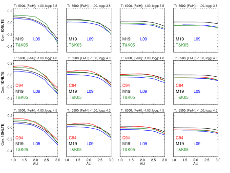
Figure 12: Same as Figure 10 but for $\mathrm{[Fe/H]}=-1.0$.

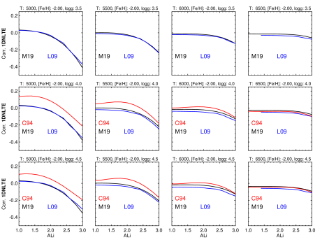
Figure 13: Same as Figure 10 but for $\mathrm{[Fe/H]}=-2.0$.

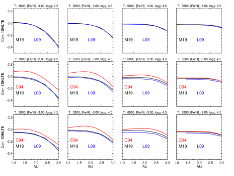
Figure 14: Same as Figure 10 but for $\mathrm{[Fe/H]}=-3.0$.

5.2 1D NLTE lithium abundance corrections in the literature

In the context of 1D NLTE lithium abundance corrections, there are a number of other authors who contributed to this topic. We refer in this section to the work by Carlsson et al. (1994), Pavlenko & Magazzu (1996), Takeda & Kawanomoto (2005) and more recently Lind et al. (2009). They all provided a series of 1D NLTE lithium abundance corrections for the lithium resonance line at 670.8 nm, and in some cases also for the subordinate line at 610.3 nm, for a diversity of stellar parameters and lithium abundances. After briefly discussing their setups and techniques, we show a comparison of the 1D NLTE lithium abundance corrections between our results and those of the following authors.

• Carlsson et al. (1994): their atmosphere grid contains one-dimensional LTE plane-parallel MARCS models (Gustafsson et al., 1975) with ${T_{\rm eff}}$ between 4500 and 7500 K, $\log g$= 0.0, 2.0, 4.0 and 4.5 and $\mathrm{[Fe/H]}=-3.0,-2.0,-1.0$, and $0.0$. The NLTE departure coefficients are computed adopting a Li model atom with 21 levels and 20 bound-bound transitions, allowing them to compute 1D NLTE lithium abundance corrections for both the resonance and the subordinate lithium lines. For the latter, however, they do not provide the values of the corrections since they are smaller and show significantly less variation across the grid than for the resonance line. The 1D NLTE corrections for the Li i $\lambda$670.8 nm line are given, for all the models of their grid, through a set of coefficients for a fourth-order polynomial fit to the values of their corrections as a function of $A$(Li). The assumed microturbulence is not specified.

• Pavlenko & Magazzu (1996): the authors compute 1D NLTE and 1D LTE synthetic lithium line profiles and CoGs for three lithium lines: the resonance doublet ($\lambda$670.8 nm) and two subordinate lines ($\lambda$610.3 nm and $\lambda$812.6 nm). They provide 1D NLTE and 1D LTE equivalent widths in tabular form for a grid of Kurucz (1993) ATLAS9 model atmospheres for solar metallicity G-M dwarfs and subgiant stars with $3500\leq T_{\rm eff}\leq 6000\,\mathrm{K}$ and $3.0\leq\log\,g\leq 4.5$ and for wide range of lithium abundances $A$(Li). Presumably, a fixed microturbulence parameter $\xi_{\rm micro}$=2.0 $\mathrm{km\leavevmode\nobreak\ s}^{-1}$is adopted (details lacking). For the coolest models of their grid ($3500\leq T_{\rm eff}\leq 4000\,\mathrm{K}$), they find a very weak dependence of NLTE line profiles (and equivalent widths) on the surface gravity. In LTE, on the other hand, this dependence is quite strong, emphasizing the importance of using NLTE results in order to minimize the unrealistic effects of errors in $\log g$  on lithium abundance determinations. For comparing these results to our corrections, we converted the LTE and NLTE equivalent widths of Pavlenko & Magazzu (1996) to 1D NLTE abundance corrections (as a function of the 1D LTE abundance) by interpolation in their CoGs.

• Takeda & Kawanomoto (2005): they employ an extensive grid of 100 Kurucz (1993) ATLAS9 model atmospheres to determine 1D NLTE lithium abundances from the lithium resonance doublet line for a sample of 160 F-K dwarfs and subgiant stars of the Galactic disc. The range of stellar parameters considered is quite large, covering $5000\leq T_{\rm eff}\leq 7000\,\mathrm{K}$, $3.0\leq\log\,g\leq 5.0$, and $-1.0\leq\mathrm{[Fe/H]}\leq+0.4$. A microturbulence parameter of $\xi_{\rm micro}$ = $1.5$ $\mathrm{km\leavevmode\nobreak\ s}^{-1}$  has been assumed across the entire grid of models. They provide grids of theoretical equivalent widths and the corresponding NLTE corrections for $A$(Li) = $0.5,1.0,1.5,2.0,2.5,3.0$ and $3.5$.

• Lind et al. (2009): this work represents the most comprehensive 1D NLTE calculations of lithium abundance and corrections in late-type stars. By using a 1D MARCS (Gustafsson et al., 2008) model atmospheres grid spanning ${T_{\rm eff}}=[4000\ldots 8000]\,\mathrm{K}$, $\log g=[1.0\ldots 5.0]$ and $\mathrm{[Fe/H]}=[0.0\ldots-3.0]$, they computed synthetic line profiles for the lithium lines at $\lambda\,670.8$ nm and $\lambda\,610.3$ nm for $A\rm(Li)=[-0.30\ldots+4.20]$. For models with $\log g\geq 3.0$ the spectra were computed adopting a microturbulence parameter $\xi_{\rm micro}$ = $1.0$ and $2.0$ $\mathrm{km\leavevmode\nobreak\ s}^{-1}$. For models with $\log g\leq 3.0$ they adopted $\xi_{\rm micro}$ = $2.0$ and $5.0$ $\mathrm{km\leavevmode\nobreak\ s}^{-1}$. The LTE and NLTE equivalent widths were obtained by numerical integration over the line profiles, from which the two curves-of-growth can be constructed. The NLTE abundance corrections for each abundance were defined as the difference between the NLTE and the LTE lithium abundance that corresponds to the same equivalent width. This corresponds to the standard definition of NLTE abundance corrections and is consistent with the definition adopted in the present work (cf. Sect. 3.1, 3.2).

  The model atom used for the calculation of the NLTE departure coefficients includes the same energy levels for neutral lithium as Carlsson et al. (1994), accounting for the hyperfine structure of $\mathrm{{}^{7}Li}$ (six components for the $\lambda$670.8 nm line, three for the $\lambda$610.3 nm line). The corrections are available either by means of tables or via web interface that, similarly to our fitting function FFI_1DNLTE, allows a quick computation of the corrections as a function of the chosen input stellar parameters (${T_{\rm eff}}$, $\log g$, $\mathrm{[Fe/H]}$), lithium abundance $A$(Li) and, in their case, microturbulence parameter $\xi_{\rm micro}$.

In Figures 10 – 14, we show the comparison between our results for the 1D NLTE $A$(Li) corrections (by applying FFI_1DNLTE) and those of the other authors described previously, for metallicities $\mathrm{[Fe/H]}=0.0,-0.5,-1.0,-2.0$ and $-3.0$. Each Figure consists in $4\times 3$ panels where different effective temperatures and gravities are shown in different rows and columns, respectively. Our results are represented by black lines, whereas the colored lines show the corrections according to the other authors, as explained by the legend of each panel. The full comparison across our grid of stellar parameters could only be done with Lind et al. (2009). The other authors cover limited or different ranges of metallicity, temperatures, and gravities and for this reason are missing in some of the comparison plots.

Our 1D NLTE corrections are based on 1D LHD spectra computed with the microturbulence parameter $\xi_{\rm micro}$  as listed in Table A. Since the microturbulence is an input parameter of the IDL routine provided by Lind et al. (2009), we can ensure that the comparison if fully consistent regarding the adopted value of $\xi_{\rm micro}$, which is especially relevant for high lithium abundances where the lines are strong and potentially affected by small-scale velocity fields in the stellar photosphere. For the comparison with the other authors, full consistency regarding the choice of $\xi_{\rm micro}$ is not enforced.

Figure 10 shows the 1D NLTE corrections for solar metallicity. This plot provides a good overview of the general trend of the corrections, since such trends are qualitatively maintained also for the other $\mathrm{[Fe/H]}$. For the coolest models (${T_{\rm eff}}=5000$ and 5500 K with $\log g$ = $3.5$ and $4.0$) the curves drop steeply when the lithium resonance line saturates at large $A$(Li) values. On the other hand, for weaker lines (low $A$(Li)) the corrections become almost independent on the lithium abundance and assume a constant value. For ${T_{\rm eff}}=5000$ K, our fitting function yields a positive 1D NLTE correction of $+0.18$ dex (black line in the upper left plot of Figure 10). The location of this knee is moving towards larger lithium abundance as the effective temperature increases, together with a flattening of the overall trend. At high metallicities ($\mathrm{[Fe/H]}=0.0,-0.5$), the corrections are seen to be almost independent of $\log g$.

The global trend of our 1D NLTE lithium abundance corrections is found to be in good agreement with the other works for every metallicity. Although some scatter can be appreciated especially at ${T_{\rm eff}}=5000$ K, our results fit well within the other curves, indicating general consistency. A systematic shift of ~0.05 dex between our results and the others samples of corrections can be noticed from ${T_{\rm eff}}=6000$ K onwards and for metallicity $0.0$ (Fig. 10), $-0.5$ (Fig. 11) and $-1.0$ (Fig. 12). The origin of this offset could be traced back to the fact that different authors choose different model atmospheres. A different choice of the model atmospheres can indeed significantly affect the derived abundance corrections. For example, Pavlenko & Magazzu (1996) and Takeda & Kawanomoto (2005) employed the same ATLAS9 models, and their results correspond quite well with each other (Fig. 10, orange and green lines). If we compare their results with Lind et al. (2009) who adopt MARCS model atmospheres (blue line in Fig. 10), we can observe some offset in the corrections. Additionally, even different versions of the same type of models can lead to significant differences in the resulting abundance corrections. This is the case for Carlsson et al. (1994) (red line in Fig. 10) and Lind et al. (2009) who both use MARCS models in which the newer version employed by latter authors includes more line opacity. As explained by Lind et al. (2009), this causes a steeper temperature gradient in the upper part of the photosphere which, in turn, leads to a higher over-ionization. For this reason, the use of newer MARCS model atmospheres introduces a systematic shift in the overall trend of the abundance corrections (towards more positive, less negative corrections with respect to the results obtained with the old MARCS models), the size of which depends, however, on the stellar parameters.

5.3 Impact of different model atmospheres

The effect of using MARCS models instead of 1D LHD models has been investigated by Harutyunyan et al. (2018). They adopted the same 1D LHD model atmospheres as in the present work and experienced a similar systematic offset in their NLTE corrections when comparing their results with Lind et al. (2009).

To understand the reason for this offset, they recomputed the 1D corrections by using one of the MARCS models of Lind et al. (Gustafsson et al., 2008) with parameters ${T_{\rm eff}}$ = $6500$ K, $\log g$ = $4.0$, $\mathrm{[Fe/H]}$ = $-1.0$. Assuming a lithium abundance of $A$(Li) = $2.0$, they found that the resulting correction was $0.055$ dex lower with respect to the value obtained by means of the corresponding 1D LHD model. Applying the same MARCS–LHD offset of $-0.055$ dex over the whole range of $A$(Li) between $1.0$ and $3.0$, their modified corrections were found to be in almost perfect agreement with the work by Lind et al. (see Fig. 15).

The result of this experiment suggests that the main responsible for the differences between our 1D NLTE abundance corrections and those of the other authors is the different choice of the input model atmospheres. In addition, other factors such as a different lithium model atom and the treatment of the relevant physical processes in the calculation of the NLTE departure coefficients (e.g., collisions with neutral hydrogen, charge transfer reactions) may also play a role.

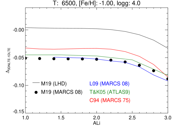
Figure 15: Comparison between our 1D NLTE $A$(Li) corrections with the other authors for the model with ${T_{\rm eff}}=6500$ K, $\log g=4.0$ and $\mathrm{[Fe/H]}=-1.0$. Our original corrections (M19, black solid line) have been shifted down (M19, black dots) by 0.055 as found by Harutyunyan et al. (2018) to account for the difference between LHD and MARCS model atmospheres. The version of the models adopted by the different authors are indicated in the legend.

6 Applications and discussion

6.1 NLTE corrections along Spite plateau

Applying our fitting functions FFI_3DNLTE and FFI_1DNLTE, we can study the influence of the different line formation models on the distribution of stars along the Spite plateau. For this purpose, we define a sample Spite plateau stars with stellar parameters in the range $5500$ K $\leq$ ${T_{\rm eff}}$ $\leq$ $6500$ K ($\Delta=20$ K), $3.5$ $\leq$ $\log g$ $\leq$ $4.5$ ($\Delta=0.5$), $-3.0$ $\leq$ $\mathrm{[Fe/H]}$ $\leq$ $-1.5$ ($\Delta=0.025$), distributed on a 3D rectangular grid. We assume that each of the $9333$ stars of the sample has the same lithium abundance of $A$(Li) = $2.2$, such that, by construction, they lie on a perfectly flat, infinitely thin Spite plateau when analyzed in 3D NLTE.

When instead analyzed in 1D LTE, the stars are distributed in a lithium abundance range $2.167\leq A$(Li) $\leq 2.268$ (see Fig. 16, star symbols). The largest negative deviation from the plateau of $-0.033$  dex is found for stars with ${T_{\rm eff}}$ = $6500$ K, $\log g$ = $3.5$, $\mathrm{[Fe/H]}$ = $-1.5$, while the most positive deviation of $+0.068$ dex is found for stars with ${T_{\rm eff}}$ = $5500$ K, $\log g$ = $4.5$, $\mathrm{[Fe/H]}$ = $-2.0$. The mean LTE Li abundance of the sample is unchanged, $A$(Li) = $2.2006$, the standard deviation is as small as $\sigma=0.0162$ dex. On the other hand, the analysis of the sample with 1D NLTE line formation is characterized by a systematic shift of the Li abundance by $-0.03$ dex to $A$(Li) = $2.17$ (see distribution of filled dots in Fig. 16). The total spread of the abundances is $\sigma=0.0134$ dex, similar to the 1D LTE case.

We conclude from this exercise that the error introduced by analyzing the Spite plateau with 1D LTE models instead of employing the full 3D NLTE machinery is small, at most $\pm 0.05$ dex in extreme cases. Our results also indicate that the 1D NLTE analysis may introduce a small systematic offset of $\Delta A$(Li) $\approx-0.03$ dex. We see no evidence that 3D and / or NLTE effects might be responsible for the “meltdown” of the Spite plateau at metallicities below $\mathrm{[Fe/H]}$ $\approx$ $-3.0$, although we cannot demonstrate this explicitly since, strictly speaking, our fitting functions are not applicable to such low metallicities.

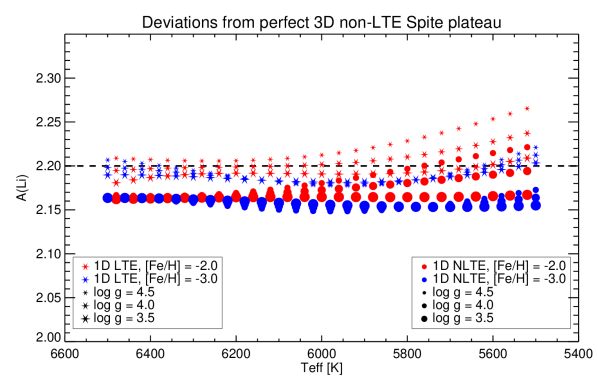
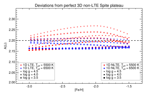
Figure 16: Lithium abundance distribution for a sample of stars with stellar parameters in the range $5500$ K $\leq$ ${T_{\rm eff}}$ $\leq$ $6500$ K, $3.5$ $\leq$ logg $\leq$ $4.5$, $-3.0$ $\leq$ $\mathrm{[Fe/H]}$ $\leq$ $-1.5$, plotted as a function of effective temperature (top) and metallicity (bottom). By construction, all stars lie on a perfectly flat, infinitely thin Spite plateau at $A$(Li)=$2.2$ when analyzed with 3D NLTE model spectra (dashed line). The corresponding 1D LTE (stars) and 1D NLTE (dots) abundances are derived by applying fitting functions FFI_3DNLTE and FFI_1DNLTE, respectively. See legend for further details.

The dependence of the corrections on ${T_{\rm eff}}$ and $\log g$ along an isochrone at metallicity $\mathrm{[Fe/H]}$ $\approx$ $-2.2$ is illustrated for three stars of globular cluster NGC 6397 studied by Nordlander et al. (2012), representing the turn-off point (TOP), the subgiant branch (SGB), and the base of the red giant branch (bRGB), respectively. The stellar parameters of these objects and their Li abundance derived in 1D NLTE, taken from Table 3 (temperature scale “100s”) of Nordlander et al. (2012), are reproduced in Cols. (1) – (5) of Table 1. With the help of our fitting functions FFI_1DNLTE and FFI_3DNLTE, we can easily estimate the 1D LTE and 3D NLTE lithium abundance, respectively, for the given 1D NLTE value. The results are collected in Cols. (6) – (7) of Table 1. We find that the 1D LTE abundance coincides with the 3D NLTE result for the TOP and (marginally) the SGB, but with the 1D NLTE result for the bRGB. Remarkably, the 3D NLTE $-$ 1D NLTE abundance difference is $+0.035$ dex for all three stars, such that all abundance gradients with ${T_{\rm eff}}$ remain perfectly unchanged. The small offset is not affecting the conclusions of Nordlander et al. (2012) whatsoever.

Table 1: Lithium abundances derived for three members of NGC 6397 with different line formation models.

Group	${T_{\rm eff}}$	$\log g$	$\mathrm{[Fe/H]}$	$A$(Li)	$A$(Li)	$A$(Li)
	[K]			1D NLTE	1D LTE	3D NLTE
TOP	$6354$	$4.01$	$-2.23$	$2.26$	$2.30$	$2.30$
SGB	$5905$	$3.71$	$-2.19$	$2.39$	$2.44$	$2.43$
bRGB	$5556$	$3.38$	$-2.13$	$1.46$	$1.46$	$1.50$

6.2 Microturbulence dependence

In this work, microturbulence is assumed to be a function of the fundamental stellar parameters according to Eq. (1). For this reason, $\xi_{\rm micro}$ is not considered as an independent parameter of our fitting functions.

The microturbulence dependence given by Eq. (1) is based on CO5BOLD 3D hydrodynamical simulations of the small-scale velocity field in stellar atmospheres and gives a reasonable approximation to empirical microturbulence trends measured in reals stars, as demonstrated by Dutra-Ferreira et al. (2016). It might nevertheless happen that the $\xi_{\rm micro}$ parameter measured in individual objects would exhibit major deviations from the adopted relation. In this case, our fitting functions FFII ($A$(Li) $\rightarrow$ EW) and FFIII (EW $\rightarrow$ $A$(Li)) would become unreliable for stronger lines whose equivalent width is susceptible to the influence of microturbulence. However, the abundance corrections are much less sensitive to $\xi_{\rm micro}$ (see, e.g., Lind et al., 2009), and the results obtained from fitting function FFI should still be valid, as long as the measured $\xi_{\rm micro}$ is used for the determination of the 1D LTE lithium abundance $A$(Li).

6.3 Blend lines

The fact that the fitting functions elaborated in this work are constructed for the pure, unblended Li feature does not imply that they cannot be applied to stars where some blend lines of other elements interfere with the lithium doublet. In this case, the EW value of the lithium resonance doublet cannot be measured directly from an observed spectrum but must be deduced by some technique to disentangle the contributions of the interfering blend lines from that of the pure lithium spectrum. This is not an uncommon procedure and there are different methods to achieve such EW extraction. For example, the solar spectrum is characterized by a weak lithium feature immersed in several blend lines. Nevertheless, Brault & Mueller (1975) succeeded in subtracting the spectrum of the blend lines (mainly the laboratory spectrum of the CN molecular band) from that of the Sun, thus isolating the lithium feature. Another technique to derive the pure Li i EW from a blended spectrum is to use the spectrum of a reference star with similar stellar parameters, but being essentially lithium-free, as a template which is subtracted from the original blended spectrum to retrieve the de-blended pure lithium line profile (e.g., Strassmeier et al. 2015, Flores Soriano et al. 2015). A necessary condition for this procedure to be valid is that all lines must be sufficiently weak, lying on the linear part of the curve-of-growth.

In general, whenever a LTE lithium abundance can be estimated from an observed spectrum, the 3D NLTE (or 1D NLTE) correction calculated with our fitting functions can be applied.

6.4 Lithium isotopic ratio

The present investigation is based on synthetic spectra that were computed for a fixed (meteoritic) lithium isotopic ratio of $\mathrm{{}^{6}Li/^{7}Li}$=8.2%, assuming that the derived abundance corrections are insensitive to this choice. For $\mathrm{[Fe/H]}$ = $0.0$ and $-2.0$, we have checked the validity of this assumption by recomputing the full set of 1D LHD spectra with $\mathrm{{}^{6}Li/^{7}Li}$=0.0, which is probably a more realistic assumption since $\mathrm{{}^{6}Li}$ is expected to be completely destroyed during the pre-main sequence evolution of the stars in the parameter range under consideration. We find that the corrections computed with $\mathrm{{}^{6}Li/^{7}Li}$=0.0 start to deviate significantly from the standard corrections ($\mathrm{{}^{6}Li/^{7}Li}$=8.2%) only for the strongest lines (EW $\ga 250$ mÅ) due to saturation effects that lead to slightly more negative corrections. In the most extreme case, the difference amounts to $-0.038$ dex (${T_{\rm eff}}$=$5000$ K, $\log g$=$3.5$, $\mathrm{[Fe/H]}$=$-2.0$, $A$(Li)=$3.0$).

The fitting functions FFI, FFII, FFIII were designed to fit the data computed with $\mathrm{{}^{6}Li/^{7}Li}$=8.2%. However, we found that they can also be used to obtain the corrections valid for $\mathrm{{}^{6}Li/^{7}Li}$=0.0 and the corresponding conversion between EW and $A$(Li) by applying an empirical shift of the input $A$(Li) (FFI, FFII) or the input EW (FFIII) as follows:

$$\Delta_{0} = \texttt{\rm FFI}\left({T_{\rm eff}},\log g,A\mathrm{(Li)+0.035}\right)$$

$$\log_{10}(\mathrm{EW}_{0}) = \texttt{FFII}\left({T_{\rm eff}},\log g,A\mathrm{(Li)+0.045}\right)-0.045$$

$$A_{0}\mathrm{(Li)} = \texttt{FFIII}\left({T_{\rm eff}},\log g,1.109\times\mathrm{EW}\right)-0.045\,,$$ (10)

where quantities with subscript $0$ indicate the results adjusted for zero $\mathrm{{}^{6}Li}$ contribution. With this modification, the fitting functions reproduce the 1D data computed with $\mathrm{{}^{6}Li/^{7}Li}$=0.0 with almost the same accuracy as the original fitting functions reproduce the data computed with $\mathrm{{}^{6}Li/^{7}Li}$=8.2%. We assume that the same manipulation works also for the intermediate metallicities as well as for the 3D case.

7 Conclusions

We extensively investigated the lithium line formation in solar-type FGK stars of different metallicity from a purely theoretical perspective. From the CIFIST grid of 3D CO5BOLD model atmospheres, we utilized a large sub-set of models and calculated 3D NLTE and 1D NLTE lithium abundance corrections from synthetic curves-of-growth, spanning a wide range of stellar parameters and lithium abundances. This allowed us to study the magnitude of such 3D and NLTE effects across the grid. The derived corrections can be applied to improve the accuracy of 1D LTE abundance determinations for stellar metallicities in the range $-3.0\leq\mathrm{[Fe/H]}\leq 0.0$.

We found these corrections to be rather small (but still significant) for weaker lines (low $A\rm(Li)_{1DLTE}$ and higher ${T_{\rm eff}}$), where they are of the order of $\pm 0.05$ dex. Their magnitude increases substantially for cooler temperatures and lower metallicities, especially for high lithium abundances ($A\rm(Li)_{1DLTE}\geq 2.0$) where the corrections can reach the $-0.30$ dex level. It is also worth noting that the abundance corrections become systematically more negative towards the more metal-poor stars (with a possible reversal of the trend near [Fe/H] = $-2.0$) for which reliable lithium abundances are of particular interest.

Since 3D model atmosphere simulations and NLTE line formation calculations are time consuming and require considerable computational resources, we first condensed the results of our study into a set of tables that provide the 3D NLTE abundance corrections as a function of the stellar parameters and the 1D LTE lithium abundance $A^{\ast}$(Li) to which the correction shall be applied. We then translated the tabulated corrections into analytical functions that evaluate the 3D NLTE or 1D NLTE corrections at arbitrary ${T_{\rm eff}}$, $\log g$, $A^{\ast}$(Li), separately for a fixed grid of metallicities $\mathrm{[Fe/H]}$. In a similar way, we also provide analytical fitting functions for directly converting a given lithium abundance into an equivalent width or vice versa, a given equivalent width into a lithium abundance (3D NLTE or 1D NLTE). The coefficients of these multi-dimensional polynomial functions are tabulated in the appendix.

For further convenience, we have developed a Python script that performs the evaluation of all six fitting functions for given ${T_{\rm eff}}$, $\log g$, $\mathrm{[Fe/H]}$, and $\mathrm{{}^{6}Li/^{7}Li}$, using the polynomial coefficients tabulated as a function of $\mathrm{[Fe/H]}$, applying the corrections for isotopic ratio if needed, and subsequently interpolating to the desired $\mathrm{[Fe/H]}$.

By means of the fitting functions developed in this work, the results of complex 3D and NLTE calculations are readily accessible and quickly applicable to large samples of stars. In this way, our work contributes to improving the accuracy of spectroscopic lithium abundance determinations across a wide range of stellar metallicities, and may thus help to address the open questions related to the lithium content in metal-poor and solar-like stellar atmospheres.

Our results confirm that for metal-poor stars on the Spite plateau, 3D and NLTE effects are by far too small to provide a solution for the cosmological lithium problem, the persistent disagreement between the stellar plateau at $A$(Li) $\approx 2.2$ and the primordial lithium abundance of $A$(Li) $\approx 2.5$ inferred from WMAP and Planck measurements of the cosmic microwave background. At the same time, the metallicity dependence of the corrections offers no explanation for the Li “meltdown” observed below [Fe/H] $\approx$ $-3.0$.

It has recently been claimed that stellar turbulent diffusion models are able to explain the lithium depletion of the Spite plateau, although their inclusion in stellar evolution models is not exempted from some uncertainties. To better constrain the underlying physics, extremely precise lithium abundance measurements along isochrones of metal-poor globular clusters are necessary. Using our fitting functions for the lithium abundance corrections, it is easy to show that differential 3D and NLTE effects between stars at the turn-off point and the base of the red giant branch are less than $0.04$ dex.

Appendix A Model atmospheres used

In Table A we compile the main properties of the full grid of models used in this work. The name of the 3D model (col. $1$) is followed by the number of opacity bins (col. $2$) and the number of representative snapshots evaluated for the respective model (col. $3$). Columns ($4$)–($6$) list the fundamental stellar parameters (${T_{\rm eff}}$, $\log g$ and $\mathrm{[Fe/H]}$) which are identical for 3D and 1D LHD models. The effective temperature reported in col. ($4$) is obtained by averaging the emergent radiative flux over the sub-sample of the selected $N_{\rm snap}$ snapshots of each CO5BOLD simulation. Finally, col. ($7$) shows the microturbulence parameter $\xi_{\rm micro}$ which is computed by means of Eq. (1) and is adopted for the spectral line profile synthesis from the 1D LHD models.

Table 2: List of the main properties of the models that have been used for developing the fitting functions. The models that are missing in the CIFIST grid (${T_{\rm eff}}=6500$ K, $\log g=3.5$) are highlighted in bold face. For these parameters we still provide values for the lithium abundance corrections by means of extrapolation from the existing models.

Model name	Opacity	Number of	${T_{\rm eff}}$	$\log g$	[Fe/H]	$\xi_{\rm micro}$
	bins	snapshots	[K]	[dex]	[dex]	[$\mathrm{km\leavevmode\nobreak\ s}^{-1}$]
d3t50g35mm00n01	5	19ss	4920	3.5	0.0	0.90
d3t50g35mm05n01	6	20ss	4960	3.5	-0.5	0.92
d3t50g35mm10n01	6	20ss	4930	3.5	-1.0	0.90
d3t50g35mm20n01	6	20ss	4980	3.5	-2.0	0.93
d3t50g35mm30n01	6	20ss	4980	3.5	-3.0	0.93
d3t50g40mm00n01	6	20ss	4950	4.0	0.0	0.82
d3t50g40mm05n01	6	20ss	5000	4.0	-0.5	0.84
d3t50g40mm10n01	6	20ss	4990	4.0	-1.0	0.84
d3t50g40mm20n01	6	20ss	4960	4.0	-2.0	0.83
d3t50g40mm30n02	6	20ss	5160	4.0	-3.0	0.89
d3t50g45mm00n04	5	20ss	4980	4.5	0.0	0.82
d3t50g45mm05n01	6	20ss	5040	4.5	-0.5	0.83
d3t50g45mm10n03	6	19ss	5060	4.5	-1.0	0.84
d3t50g45mm20n03	6	19ss	5010	4.5	-2.0	0.83
d3t50g45mm30n03	6	20ss	4990	4.5	-3.0	0.82
d3t55g35mm00n01	5	18ss	5430	3.5	0.0	1.13
d3t55g35mm05n01	6	20ss	5470	3.5	-0.5	1.15
d3t55g35mm10n01	6	19ss	5480	3.5	-1.0	1.16
d3t55g35mm20n01	6	20ss	5500	3.5	-2.0	1.17
d3t55g35mm30n01	6	20ss	5540	3.5	-3.0	1.18
d3t55g40mm00n01	5	20ss	5480	4.0	0.0	0.99
d3t55g40mm05n01	6	19ss	5530	4.0	-0.5	1.01
d3t55g40mm10n01	6	20ss	5530	4.0	-1.0	1.01
d3t55g40mm20n01	6	20ss	5470	4.0	-2.0	0.99
d3t55g40mm30n01	6	20ss	5480	4.0	-3.0	0.99
d3t55g45mm00n01	5	20ss	5490	4.5	0.0	0.91
d3t55g45mm05n01	6	20ss	5460	4.5	-0.5	0.91
d3t55g45mm10n01	6	20ss	5470	4.5	-1.0	0.91
d3t55g45mm20n01	6	20ss	5480	4.5	-2.0	0.91
d3t55g45mm30n01	6	20ss	5490	4.5	-3.0	0.91
d3t59g35mm00n01	5	20ss	5880	3.5	0.0	1.34
d3t59g35mm05n02	6	20ss	5760	3.5	-0.5	1.29
d3t59g35mm10n01	6	20ss	5890	3.5	-1.0	1.34
d3t59g35mm20n01	6	20ss	5860	3.5	-2.0	1.33
d3t59g35mm30n01	6	20ss	5870	3.5	-3.0	1.34
d3t59g40mm00n01	5	18ss	5930	4.0	0.0	1.13
d3t59g40mm05n01	6	20ss	5920	4.0	-0.5	1.13
d3t59g40mm10n02	6	20ss	5850	4.0	-1.0	1.11
d3t59g40mm20n02	6	20ss	5860	4.0	-2.0	1.11
d3t59g40mm30n02	6	20ss	5850	4.0	-3.0	1.11
d3t59g45mm00n01	5	19ss	5870	4.5	0.0	0.98
d3t59g45mm05n01	6	20ss	5900	4.5	-0.5	0.98
d3t59g45mm10n01	6	08ss	5920	4.5	-1.0	0.99
d3t59g45mm20n01	6	18ss	5920	4.5	-2.0	0.99
d3t59g45mm30n01	6	19ss	5920	4.5	-3.0	0.99
d3t63g35mm00n01	5	21ss	6130	3.5	0.0	1.45
d3t63g35mm05n02	6	20ss	6150	3.5	-0.5	1.46
d3t63g35mm10n01	6	20ss	6210	3.5	-1.0	1.49
d3t63g35mm20n01	6	20ss	6290	3.5	-2.0	1.53
d3t63g35mm30n01	6	20ss	6310	3.5	-3.0	1.54
d3t63g40mm00n01	5	20ss	6230	4.0	0.0	1.23
d3t63g40mm05n01	6	20ss	6250	4.0	-0.5	1.24
d3t63g40mm10n01	6	20ss	6260	4.0	-1.0	1.24
d3t63g40mm20n01	6	16ss	6280	4.0	-2.0	1.24
d3t63g40mm30n01	6	20ss	6270	4.0	-3.0	1.24

Table 2: …continued.

Appendix B Coefficients

In this appendix we tabulate the numerical coefficients for the fitting functions provided in this work. In all of the following tables, the first column contains the name of each numerical coefficient and in the next five columns their numerical value for each one of the five metallicities of our grid.

B.1 Fitting functions FFI

Tables 3 and 4 list the coefficients $\mathrm{c}_{ijk}$ defined by Eq. (6) for FFI_3DNLTE and FFI_1DNLTE, respectively. Figure 17 gives an overview of the fitting function errors at the nodes of the grid for all metallicities, while Figure 18 illustrates the interpolation errors evaluated on a refined temperature grid of 1D LHD models for [Fe/H] = $0.0$ and $-2.0$.

Table 3: Numerical coefficients $c_{ijk}$ of the fitting function FFI_3DNLTE approximating the 3D NLTE lithium abundance corrections $\Delta_{\rm 3DNLTE-1DLTE}$ (Eq. 6) for the five metallicities of our grid.

$\mathrm{c}_{ijk}$	$\mathrm{[Fe/H]}$
	0.0 dex	-0.5 dex	-1.0 dex	-2.0 dex	-3.0 dex
c000	0.1934700	0.1137574	0.1059171	0.0110396	0.0302943
c100	-0.0239075	-0.0257894	-0.0307899	-0.0160289	-0.0730075
c001	-0.1479080	-0.1209572	-0.1251443	0.0061589	-0.0496778
c101	0.1187087	-0.0034667	0.1605346	-0.2109836	0.1059637
c002	0.1429609	0.2182036	0.1630807	0.1021026	0.1900663
c102	-0.3658550	0.0199786	-0.4815992	0.3694110	0.0988528
c003	-0.1536380	-0.2343304	-0.1063167	-0.1538708	-0.2032447
c103	0.3933365	0.0043123	0.4460331	-0.1835116	-0.2011892
c004	0.0504229	0.0804113	0.0225933	0.0569504	0.0615852
c104	-0.1317260	-0.0116685	-0.1317514	0.0189035	0.0706434
c010	-0.0112007	-0.0095449	-0.0071110	-0.0101823	-0.0140992
c110	0.0014934	0.0041522	-0.0008530	0.0101311	0.0110694
c011	-0.0157936	-0.0057599	-0.0049469	0.0077487	0.0031318
c111	-0.0035633	-0.0132778	-0.0108938	-0.0188577	0.0021892
c012	-0.0029972	-0.0097395	-0.0218368	-0.0330288	-0.0016796
c112	0.0015286	0.0149844	0.0249090	0.0265209	0.0200220
c013	0.0226405	0.0190282	0.0262789	0.0303408	0.0146414
c113	-0.0007266	-0.0054095	-0.0108755	-0.0155570	-0.0209639
c020	0.0228360	0.0220577	0.0198897	0.0230061	0.0223846
c120	0.0001464	-0.0048820	-0.0002827	-0.0148570	-0.0242930
c021	-0.0015479	-0.0023546	0.0026504	-0.0048869	-0.0188727
c121	0.0028341	0.0042002	-0.0048818	0.0090188	-0.0036151
c022	-0.0304533	-0.0255947	-0.0278502	-0.0282937	-0.0237323
c122	-0.0001805	-0.0008105	0.0014137	0.0056108	0.0164049
c030	-0.0047771	-0.0070773	-0.0069892	-0.0073567	-0.0025587
c130	-0.0015685	0.0022109	0.0023593	0.0061664	0.0125796
c031	0.0190796	0.0192168	0.0190010	0.0229878	0.0236960
c131	-0.0001362	-0.0008104	0.0003031	-0.0062793	-0.0082827
c040	-0.0040627	-0.0040545	-0.0040723	-0.0051027	-0.0060987
c140	0.0002129	-0.0004152	-0.0006280	-0.0000427	-0.0006542

Table 4: Numerical coefficients $c_{ijk}$ for the fitting function FFI_1DNLTE approximating the 1D NLTE lithium abundance corrections $\Delta_{\rm 1DNLTE-1DLTE}$ (Eq. 6) for the five metallicities of our grid.

$\mathrm{c}_{ijk}$	$\mathrm{[Fe/H]}$
	0.0 dex	-0.5 dex	-1.0 dex	-2.0 dex	-3.0 dex
c000	0.1791557	0.1050792	0.0990588	0.0328342	0.0124536
c100	-0.0073790	-0.0084633	-0.0070312	-0.0032602	-0.0587628
c001	-0.1406743	-0.1530184	-0.2250787	-0.1734033	-0.0807081
c101	0.0561255	0.0583358	0.1517873	0.0513971	0.2173629
c002	0.1231245	0.2275670	0.4254515	0.3390962	0.1571438
c102	-0.1741239	-0.1280650	-0.4558604	-0.1418215	-0.2973344
c003	-0.1497231	-0.1886872	-0.3898447	-0.2990925	-0.1397715
c103	0.1935423	0.0873244	0.4176210	0.1312618	0.1654042
c004	0.0536468	0.0499225	0.1203871	0.0905645	0.0401296
c104	-0.0675082	-0.0183153	-0.1236082	-0.0432368	-0.0335796
c010	-0.0111539	-0.0073209	-0.0051128	-0.0041143	-0.0080132
c110	0.0046478	0.0038263	0.0008493	0.0058993	0.0047513
c011	-0.0042783	0.0023326	0.0007908	-0.0005678	-0.0023488
c111	-0.0146549	-0.0232104	-0.0205851	-0.0043562	0.0108387
c012	-0.0085580	-0.0180569	-0.0272235	-0.0223643	0.0063592
c112	0.0069384	0.0264662	0.0329991	0.0043666	0.0036971
c013	0.0196931	0.0185953	0.0255633	0.0231517	0.0073388
c113	0.0002411	-0.0085541	-0.0130252	-0.0057535	-0.0107872
c020	0.0216719	0.0188139	0.0160754	0.0149103	0.0149583
c120	-0.0036719	-0.0032942	-0.0003223	-0.0091198	-0.0155050
c021	-0.0064836	-0.0034779	0.0022292	0.0004144	-0.0149522
c121	0.0096988	0.0076570	0.0005769	0.0071321	-0.0049674
c022	-0.0249244	-0.0211086	-0.0245816	-0.0255060	-0.0194343
c122	-0.0038088	-0.0031284	-0.0005112	0.0051264	0.0128407
c030	-0.0052306	-0.0068116	-0.0056458	-0.0046855	-0.0006729
c130	0.0006315	0.0013540	0.0010385	0.0028883	0.0091173
c031	0.0188565	0.0183322	0.0181051	0.0205227	0.0213070
c131	-0.0010174	-0.0012430	-0.0004732	-0.0056278	-0.0069360
c040	-0.0040438	-0.0040839	-0.0043396	-0.0054409	-0.0063454
c140	-0.0000474	-0.0001415	-0.0001646	0.0006245	-0.0001072

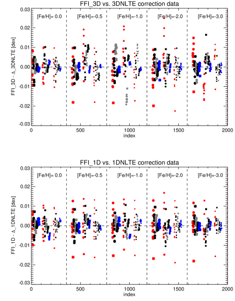
Figure 17: Performance of the Li abundance correction fitting functions FFI_3DNLTE (top) and FFI_1DNLTE (bottom). For each metallicity, a total of $165$ points indicates the difference (FFI $-$ input correction) as a function of an index that runs over $A$(Li), ${T_{\rm eff}}$, and $\log g$. Large (left group), intermediate (middle group), and small dots (right group) correspond to $\log g$ = $3.5$, $4.0$, and $4.5$, respectively. For each gravity, ${T_{\rm eff}}$ increases from left to right ($5000$ K: red, $5500$ K: black, $5900$ K: gray, $6300$ K: black, $6500$ K: blue). Each effective temperature is represented by $10$ dots indicating the results for $1.0\leq A$(Li) $\leq 2.8$ plus a square for $A$(Li) = $3.0$.

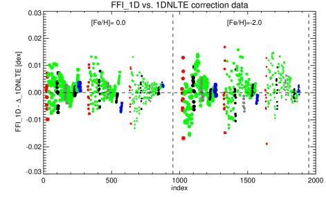
Figure 18: Partial view of Fig. 17 (bottom), showing for metallicities [Fe/H] = $0.0$ and $-2.0$ the difference (FFI${}_{\rm 1DNLTE}-$ input correction) as a function of spectrum number, now for a refined temperature grid with $\Delta$${T_{\rm eff}}$ = $100$ K. For each metallicity, large, intermediate, and small dots correspond to $\log g$ = $3.5$, $4.0$, and $4.5$, respectively. For each gravity, ${T_{\rm eff}}$ increases from left to right. Color coding for the temperatures of the original grid is the same as in Fig. 17; in addition, green dots represent the results for the intermediate 1D LHD test models. As before, each effective temperature is represented by $10$ dots for $1.0\leq A$(Li) $\leq 2.8$ plus a square for $A$(Li) = $3.0$.

B.2 Fitting functions FFII

Tables 5 and 6 contain the coefficients $\mathrm{w}_{ijk}$ defined by Eq. (7) for the equivalent width fitting functions FFII_3DNLTE and FFII_1DNLTE, respectively. Figure 19 gives an overview of the fitting function errors at the nodes of the grid for all metallicities, while Figure 20 illustrates the interpolation errors evaluated on a refined temperature grid of 1D LHD models for [Fe/H] = $0.0$ and $-2.0$.

Table 5: Numerical coefficients $w_{ijk}$ (Eq. 7) for the equivalent width fitting function FFII_3DNLTE, derived for the five metallicities of our grid.

$\mathrm{w}_{ijk}$	$\mathrm{[Fe/H]}$
	0.0 dex	-0.5 dex	-1.0 dex	-2.0 dex	-3.0 dex
w000	0.1475069	0.2245458	0.2239167	0.2849084	0.2068955
w100	0.0347089	0.0339855	0.0306456	0.0223937	0.0133552
w001	-1.0208849	-1.1469250	-1.2259755	-1.3272777	-0.9932886
w101	-0.0669732	0.1537401	0.2371681	0.3296509	0.1479368
w002	0.2054467	0.5791591	0.7219083	0.8228920	0.4085410
w102	0.2143639	-0.2905753	-0.4994409	-0.6173923	-0.3156809
w003	0.0014179	-0.2833503	-0.3976060	-0.3689554	-0.2145625
w103	-0.2303063	0.1320859	0.3419425	0.3533569	0.2474548
w004	-0.0188241	0.0516219	0.0878278	0.0580685	0.0553802
w104	0.0782668	-0.0003866	-0.0704236	-0.0529642	-0.0656191
w010	1.0254700	1.0536114	1.0482122	1.0525770	1.0448927
w110	-0.0123804	-0.0402674	-0.0328853	-0.0274988	-0.0895899
w011	-0.0370201	-0.0563704	-0.0354928	-0.0487050	-0.0955188
w111	-0.0224963	-0.0349607	-0.0656007	-0.0428780	0.0236516
w012	-0.1005337	-0.1450037	-0.1672949	-0.2049884	-0.0942996
w112	0.0257704	0.0782432	0.0999685	0.0993408	0.0422533
w013	0.0385082	0.0430121	0.0515689	0.0606149	0.0203157
w113	-0.0049530	-0.0276824	-0.0309441	-0.0416862	-0.0082573
w020	-0.0012442	-0.0111443	-0.0123488	-0.0087517	-0.0016854
w120	0.0115008	0.0312578	0.0315381	0.0227707	0.0650281
w021	0.0727088	0.1046035	0.1053274	0.1329422	0.1065020
w121	0.0038124	-0.0052565	-0.0022758	-0.0118978	-0.0372886
w022	-0.0223655	-0.0130742	-0.0143628	-0.0106278	-0.0077959
w122	-0.0049537	-0.0047638	-0.0063133	0.0020711	-0.0033688
w030	-0.0159346	-0.0212027	-0.0199292	-0.0273466	-0.0233474
w130	-0.0035786	-0.0086870	-0.0090606	-0.0054171	-0.0138632
w031	0.0101170	0.0031635	0.0027428	-0.0033878	-0.0005013
w131	0.0004436	0.0013816	0.0015143	0.0004107	0.0057651
w040	-0.0033853	-0.0021711	-0.0022738	-0.0007230	-0.0017665
w140	0.0002804	0.0008126	0.0008187	0.0006392	0.0011240

Table 6: Numerical coefficients $w_{ijk}$ (Eq. 7) for the equivalent width fitting function FFII_1DNLTE, derived for the five metallicities of our grid.

$\mathrm{w}_{ijk}$	$\mathrm{[Fe/H]}$
	0.0 dex	-0.5 dex	-1.0 dex	-2.0 dex	-3.0 dex
w000	0.1668157	0.2358674	0.2338765	0.2696325	0.2404062
w100	0.0149293	0.0173628	0.0081412	0.0048003	-0.0302344
w001	-1.0165459	-1.1335444	-1.0981356	-1.1334040	-0.9817465
w101	-0.0210521	0.1219691	0.2055447	0.0515904	0.0651075
w002	0.1444629	0.6690733	0.3493729	0.5578882	0.4516058
w102	0.1364904	-0.2768881	-0.3623220	-0.0860166	0.0226130
w003	0.1038219	-0.4558280	0.0130863	-0.2255391	-0.2897598
w103	-0.1815287	0.2097250	0.1752576	0.0647830	-0.0531376
w004	-0.0652711	0.1265842	-0.0550262	0.0308042	0.0826828
w104	0.0725737	-0.0500634	-0.0108072	-0.0134427	0.0153335
w010	1.0132868	1.0417293	1.0374104	1.0327493	1.0081008
w110	-0.0064728	-0.0379439	-0.0345743	-0.0132608	-0.0198091
w011	-0.0207368	-0.0674934	-0.0327851	-0.0506050	-0.0586258
w111	-0.0421332	-0.0226979	-0.0642451	-0.0323514	-0.0026935
w012	-0.1076595	-0.1195333	-0.1635718	-0.1613043	-0.0994343
w112	0.0420931	0.0555183	0.1068789	0.0442803	0.0442668
w013	0.0443194	0.0354617	0.0530645	0.0442895	0.0199720
w113	-0.0087720	-0.0160399	-0.0309735	-0.0087144	-0.0101419
w020	0.0064495	-0.0006828	-0.0036903	0.0062150	0.0227895
w120	0.0083023	0.0282699	0.0317697	0.0112594	0.0099326
w021	0.0627791	0.0999068	0.0990063	0.1104659	0.0848678
w121	0.0091549	-0.0062510	-0.0082175	-0.0011886	-0.0238849
w022	-0.0242035	-0.0155056	-0.0155906	-0.0093547	-0.0059664
w122	-0.0067343	-0.0054689	-0.0079125	-0.0053423	-0.0008217
w030	-0.0166254	-0.0235642	-0.0215853	-0.0282541	-0.0286804
w130	-0.0027657	-0.0069611	-0.0073040	-0.0009272	0.0041802
w031	0.0127171	0.0048428	0.0042163	0.0004064	0.0033798
w131	-0.0003911	0.0015833	0.0030302	0.0002764	0.0023297
w040	-0.0036484	-0.0021369	-0.0023126	-0.0012000	-0.0016354
w140	0.0002877	0.0005860	0.0004177	0.0000390	-0.0008902

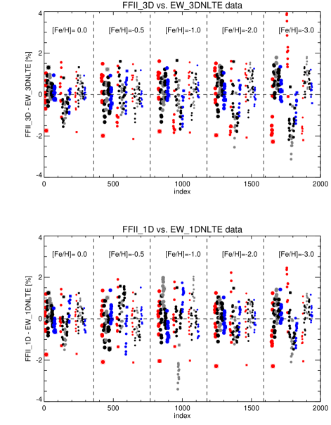
Figure 19: Performance of the Li equivalent width fitting functions FFII_3DNLTE (top) and FFII_1DNLTE (bottom). For each metallicity, a total of $165$ points indicates the relative difference (FFII $-$ input EW) as a function of an index that runs over $A$(Li), ${T_{\rm eff}}$, and $\log g$. Large (left group), intermediate (middle group), and small dots (right group) correspond to $\log g$ = $3.5$, $4.0$, and $4.5$, respectively. For each gravity, ${T_{\rm eff}}$ increases from left to right ($5000$ K: red, $5500$ K: black, $5900$ K: gray, $6300$ K: black, $6500$ K: blue). Each effective temperature is represented by $10$ dots indicating the results for $1.0\leq A$(Li) $\leq 2.8$ plus a square for $A$(Li) = $3.0$.

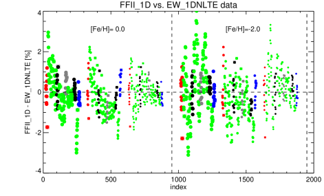
Figure 20: Partial view of Fig. 19 (bottom), showing for metallicities [Fe/H] = $0.0$ and $-2.0$ the difference (FFII${}_{\rm 1DNLTE}-$ input EW) as a function of spectrum number, now for a refined temperature grid with $\Delta$${T_{\rm eff}}$ = $100$ K. For each metallicity, large, intermediate, and small dots correspond to $\log g$ = $3.5$, $4.0$, and $4.5$, respectively. For each gravity, ${T_{\rm eff}}$ increases from left to right. Color coding for the temperatures of the original grid is the same as in Fig. 19; in addition, green dots represent the results for the intermediate 1D LHD test models. As before, each effective temperature is represented by $10$ dots for $1.0\leq A$(Li) $\leq 2.8$ plus a square for $A$(Li) = $3.0$.

B.3 Fitting functions FFIII

In the context of the “inverse” fitting function FFIII, the coefficients $p_{m}$ and $q_{m}$ needed for the normalization of the input equivalent width according to Eq. (8), are listed in Table 7. The coefficients $\mathrm{a}_{ijk}$ for the related fitting function (Eq. 9) are presented in Table 8 for the 3D case and in Table 9 for the 1D case. Figure 21 gives an overview of the fitting function errors at the nodes of the grid for all metallicities, while Figure 22 illustrates the interpolation errors evaluated on a refined temperature grid of 1D LHD models for [Fe/H] = $0.0$ and $-2.0$.

Table 7: Numerical coefficients for the parabolic functions $p(z)$ and $q(z)$ for the scaling of the EW values (Eq. 8) for the five metallicities of our grid.

	3D NLTE
	0.0 dex	-0.5 dex	-1.0 dex	-2.0 dex	-3.0 dex
$p_{0}$	1.1666957	1.2504734	1.2464725	1.3043333	1.2126223
$p_{1}$	-0.9744305	-0.9486030	-0.9792976	-1.0051502	-0.8792871
$p_{2}$	0.0998992	0.0860085	0.1103587	0.1234108	0.0831803
$q_{0}$	2.5298152	2.5573504	2.5622675	2.6001840	2.5832374
$q_{1}$	-0.3196788	-0.2843448	-0.3114402	-0.3440792	-0.3490530
$q_{2}$	-0.0940990	-0.0961721	-0.0804780	-0.0614842	-0.0479861
	1D NLTE
	0.0 dex	-0.5 dex	-1.0 dex	-2.0 dex	-3.0 dex
$p_{0}$	1.1717118	1.2508765	1.2407464	1.2765080	1.2212788
$p_{1}$	-0.9636974	-0.9391062	-0.9457412	-0.9397265	-0.8184223
$p_{2}$	0.0969080	0.0888007	0.1022377	0.1074416	0.0538786
$q_{0}$	2.5373471	2.5629222	2.5642192	2.5933402	2.5898440
$q_{1}$	-0.3065712	-0.2770424	-0.2907207	-0.3123179	-0.3037169
$q_{2}$	-0.0994211	-0.0945872	-0.0840242	-0.0640284	-0.0647640

Table 8: Numerical coefficients $a_{ijk}$ for the fitting function FFIII_3DNLTE (Eq. 9) for the five metallicities of our grid.

$\mathrm{a}_{ijk}$	$\mathrm{[Fe/H]}$
	0.0 dex	-0.5 dex	-1.0 dex	-2.0 dex	-3.0 dex
a000	1.0129539	1.0048051	1.0073185	1.0018589	0.9843768
a100	-0.0320762	-0.0181588	-0.0225066	-0.0135131	0.0258085
a001	-0.0047474	0.1561165	0.1868200	0.2595673	0.1117859
a101	0.0966525	-0.1225815	-0.1843958	-0.2946401	-0.1551465
a002	0.0107189	-0.3957869	-0.4996260	-0.5756683	-0.2655631
a102	-0.2652379	0.2545796	0.4620044	0.6000681	0.3281206
a003	-0.0300389	0.3105966	0.4199568	0.4078356	0.2412711
a103	0.2674269	-0.1445944	-0.3654113	-0.4031672	-0.2896941
a004	0.0199194	-0.0706069	-0.1063437	-0.0853998	-0.0668322
a104	-0.0896722	0.0127179	0.0855543	0.0816975	0.0796513
a010	1.4826018	1.4363913	1.4479415	1.4363663	1.4851382
a110	-0.0122440	-0.0120726	-0.0224080	-0.0332608	-0.0266341
a011	0.4809866	0.4890558	0.4584515	0.4533793	0.3895906
a111	0.0315554	0.0315003	0.0671112	0.0233328	0.0026447
a012	-0.1093419	-0.1443315	-0.0745938	-0.0858786	-0.1282260
a112	-0.0582297	-0.0676528	-0.1250455	-0.0366054	0.0103118
a013	-0.0811257	-0.0608838	-0.0967849	-0.0887680	-0.0404274
a113	0.0315529	0.0419535	0.0693063	0.0455033	0.0214958
a020	0.0397534	0.0658588	0.0650056	0.0664652	0.0979962
a120	0.0310409	0.0362215	0.0456162	0.0816874	0.0243971
a021	0.2289434	0.3330445	0.2619056	0.2722017	0.3058020
a121	0.0119482	-0.0044280	0.0319514	-0.0529941	-0.0511880
a022	0.2664408	0.2528331	0.2841167	0.2869350	0.2237575
a122	-0.0300937	-0.0414550	-0.0792486	-0.1155353	-0.1034352
a030	-0.3033826	-0.4262138	-0.3866560	-0.3930803	-0.4543772
a130	-0.0669515	-0.0577996	-0.0822305	-0.0379099	0.0486115
a031	-0.7817028	-0.8713536	-0.8517458	-0.8782503	-0.7977752
a131	0.0597030	0.1003228	0.1256164	0.2541338	0.2421975
a040	0.7897918	0.9366162	0.9056341	0.9497166	0.9366128
a140	-0.0023798	-0.0321545	-0.0377751	-0.1493477	-0.1960495

Table 9: Numerical coefficients $a_{ijk}$ for the fitting function FFIII_1DNLTE (Eq. 9) for the five metallicities of our grid.

$\mathrm{a}_{ijk}$	$\mathrm{[Fe/H]}$
	0.0 dex	-0.5 dex	-1.0 dex	-2.0 dex	-3.0 dex
a000	1.0034880	0.9969588	0.9946962	0.9947520	0.9761783
a100	-0.0149131	-0.0012568	0.0012896	-0.0014573	0.0395208
a001	-0.0070700	0.1701429	0.0837970	0.1427269	0.1456125
a101	0.0600870	-0.1039627	-0.1483714	-0.0204912	-0.0444751
a002	0.0778053	-0.5129522	-0.1001108	-0.3366641	-0.3424794
a102	-0.1876247	0.2598852	0.3102002	0.0590798	-0.0621787
a003	-0.1373179	0.4948993	-0.0283389	0.2445354	0.3244218
a103	0.2092790	-0.2249752	-0.1888596	-0.0636695	0.0678418
a004	0.0658496	-0.1461374	0.0473187	-0.0465606	-0.0964052
a104	-0.0800654	0.0586372	0.0229167	0.0126802	-0.0208056
a010	1.4863001	1.4397544	1.4525720	1.4504639	1.4938299
a110	-0.0129561	-0.0107809	-0.0196197	-0.0334373	-0.0392963
a011	0.4811911	0.4921130	0.4573048	0.4333948	0.3481754
a111	0.0435972	0.0324621	0.0619665	0.0383781	0.0388136
a012	-0.1143308	-0.1531218	-0.0943043	-0.1027095	-0.1124205
a112	-0.0699413	-0.0597135	-0.1132561	-0.0532867	-0.0459816
a013	-0.0831284	-0.0613116	-0.0878985	-0.0772232	-0.0415169
a113	0.0356960	0.0364476	0.0626087	0.0514719	0.0511127
a020	0.0323323	0.0641480	0.0701729	0.0757278	0.0785333
a120	0.0297583	0.0277220	0.0287614	0.0668523	0.0775074
a021	0.2677503	0.3584981	0.3004327	0.3354400	0.4029507
a121	-0.0101038	-0.0243102	0.0291790	-0.0641447	-0.0807435
a022	0.2705392	0.2603878	0.2783551	0.2747025	0.2155212
a122	-0.0249536	-0.0318485	-0.0715133	-0.1116670	-0.1230486
a030	-0.3389264	-0.4639441	-0.4374807	-0.4779056	-0.5137561
a130	-0.0418873	-0.0263805	-0.0514110	-0.0003870	0.0050233
a031	-0.8119198	-0.8934028	-0.8646667	-0.8982424	-0.8600781
a131	0.0660941	0.0973589	0.1099220	0.2498231	0.2818613
a040	0.8224663	0.9672014	0.9390500	1.0030741	1.0015136
a140	-0.0164435	-0.0449689	-0.0440915	-0.1620551	-0.1865475

Figure 21: Performance of the NLTE Li abundance fitting functions FFIII_3DNLTE (top) and FFIII_1DNLTE (bottom). For each metallicity, a total of $165$ points indicates the difference (FFIII $-$ input abundance) as a function of an index that runs over $A$(Li), ${T_{\rm eff}}$, and $\log g$. Large (left group), intermediate (middle group), and small dots (right group) correspond to $\log g$ = $3.5$, $4.0$, and $4.5$, respectively. For each gravity, ${T_{\rm eff}}$ increases from left to right ($5000$ K: red, $5500$ K: black, $5900$ K: gray, $6300$ K: black, $6500$ K: blue). Each effective temperature is represented by $10$ dots indicating the results for $1.0\leq A$(Li) $\leq 2.8$ plus a square for $A$(Li) = $3.0$.

Figure 22: Partial view of Fig. 21 (bottom), showing for metallicities [Fe/H] = $0.0$ and $-2.0$ the difference (FFIII${}_{\rm 1DNLTE}-$ input abundance) as a function of spectrum number, now for a refined temperature grid with $\Delta$${T_{\rm eff}}$ = $100$ K. For each metallicity, large, intermediate, and small dots correspond to $\log g$ = $3.5$, $4.0$, and $4.5$, respectively. For each gravity, ${T_{\rm eff}}$ increases from left to right. Color coding for the temperatures of the original grid is the same as in Fig. 21; in addition, green dots represent the results for the intermediate 1D LHD test models. As before, each effective temperature is represented by $10$ dots for $1.0\leq A$(Li) $\leq 2.8$ plus a square for $A$(Li) = $3.0$.