New approach to lattice QCD at finite density; results for the critical end point on coarse lattices

Abstract

All approaches currently used to study finite baryon density lattice QCD suffer from uncontrolled systematic uncertainties in addition to the well-known sign problem. We formulate and test an algorithm, sign reweighting, that works directly at finite $\mu=\mu_{B}/3$ and is yet free from any such uncontrolled systematics. With this algorithm the only problem is the sign problem itself. This approach involves the generation of configurations with the positive fermionic weight $|{\rm Re\,}{\rm det\,}D(\mu)|$ where $D(\mu)$ is the Dirac matrix and the signs ${\rm sign}({\rm Re\,}{\rm det\,}D(\mu))=\pm 1$ are handled by a discrete reweighting. Hence there are only two sectors, $+1$ and $-1$ and as long as the average $\langle\pm 1\rangle\neq 0$ (with respect to the positive weight) this discrete reweighting by the signs carries no overlap problem and the results are reliable. The approach is tested on $N_{t}=4$ lattices with $2+1$ flavors and physical quark masses using the unimproved staggered discretization. By measuring the Fisher (sometimes also called Lee-Yang) zeros in the bare coupling on spatial lattices $L/a=8,10,12$ we conclude that the cross-over present at $\mu=0$ becomes stronger at $\mu>0$ and is consistent with a true phase transition at around $\mu_{B}/T\sim 2.4$.

1 Introduction

The numerical simulation of lattice QCD at finite baryon chemical potential is known to be hindered by the notorious sign problem: the fermionic determinant is not real and hence importance sampling techniques do not apply. Ways around the problem were nonetheless devised. These include Taylor expansion Allton:2002zi ; Gavai:2003mf ; Gavai:2004sd ; Allton:2005gk ; Gavai:2008zr ; Basak:2009uv ; Borsanyi:2011sw ; Borsanyi:2012cr ; Bellwied:2015lba ; Ding:2015fca ; Bazavov:2017dus ; Bazavov:2018mes ; Giordano:2019slo ; Bazavov:2020bjn around $\mu=\mu_{B}/3=0$, simulating at imaginary chemical potential deForcrand:2002hgr ; DElia:2002tig ; DElia:2009pdy ; Cea:2014xva ; Bonati:2014kpa ; Cea:2015cya ; Bonati:2015bha ; Bellwied:2015rza ; DElia:2016jqh ; Gunther:2016vcp ; Alba:2017mqu ; Vovchenko:2017xad ; Bonati:2018nut ; Borsanyi:2018grb ; Bellwied:2019pxh ; Borsanyi:2020fev , complex Langevin approach Seiler:2012wz ; Sexty:2013ica ; Aarts:2014bwa ; Fodor:2015doa ; Sexty:2019vqx ; Kogut:2019qmi ; Scherzer:2020kiu and reweighting Hasenfratz:1991ax ; Barbour:1997ej ; Fodor:2001au ; Fodor:2001pe ; Fodor:2004nz ; Giordano:2019gev from $\mu=0$. All of these approaches share the feature that for infinitesimally small $\mu$ at fixed spatial volume they are all expected to give correct results. Once $\mu$ is not infinitesimally small all approaches suffer from uncontrolled systematic uncertainties which render them unreliable.

More precisely, the Taylor expansion method for non-infinitesimal $\mu$ requires the computation of high order $\mu$-derivatives at $\mu=0$. It has the advantage that it provides well-defined physical quantities, namely the cumulants of the baryon number distribution at $\mu=0$ directly. However, the measurement itself leads to ever growing cancellations among fermion contractions as the order of the derivative increases. Furthermore even if a potentially large number of Taylor coefficients are computed with acceptable statistical uncertainty, the best case scenario is a reliable estimate of the radius of convergence. The Taylor expansion method will only provide information within this radius and extrapolation beyond it necessarily will involve uncontrolled systematics.

The second extrapolation method mentioned above involves simulating at imaginary $\mu$ where there is no sign problem, but the extrapolation from negative $\mu^{2}$ to positive finite $\mu^{2}$ requires assumptions about the functional form of the $\mu^{2}$ dependence. This leads again to uncontrolled systematic uncertainty in the extrapolation, similar to the case of the Taylor method.

The third popular method, the complex Langevin approach, is appealing because it is set up at finite $\mu$ directly but the precise set of necessary and sufficient conditions for it to give the correct result in QCD is so far unknown. A set of sufficient conditions for the correctness of the algorithm in general (some a priori, such as the holomorphicity of the action, and some a posteriori, such as the quick decay of the field distributions at infinity) has been proven Aarts:2009uq ; Aarts:2011ax , however these conditions are not satisfied in lattice QCD. Although one may formulate various tests of incorrectness and the lack of observed such signals may boost confidence in the correctness of the results, the systematic uncertainties associated with the potential breakdown of the algorithm cannot be estimated quantitatively. Numerical investigations indicate that present incarnations of the method break down at low temperatures. Whether an extension of the method capable of simulating also at low temperatures exists is a matter of ongoing research.

Finally the fourth method, reweighting from $\mu=0$, leads to the well-known overlap problem at some finite $\mu$. This means that if a suitable weight is found, $w(\mu)$, which may depend on any number of further parameters Fodor:2001au ; Fodor:2001pe beyond $\mu$, and expectation values are computed via $\langle{\cal O}\rangle_{\mu}=\langle{\cal O}w(\mu)\rangle_{0}/\langle w(\mu)\rangle_{0}$, then the histogram of $w(\mu)$ becomes wider and wider for increasing $\mu$. Sampling the tail of the histogram becomes eventually prohibitively expensive and a reliable error estimate at finite statistics impossible. Furthermore, there is no sharply defined condition which would signal the presence of the overlap problem or absence thereof. In practice one may attempt to confirm the lack of the overlap problem from various statistical observations and may very well obtain reliable results, but the inherent systematic uncertainty will nevertheless linger.

Our motivation for the present paper is to devise an algorithm which is free of uncontrolled systematic uncertainties and has a well-defined set of conditions for its applicability. In other words we would like to have a trustworthy algorithm in the sense that results obtained with it are reliable with well-defined statistical uncertainties and have quantifiable, controlled systematic uncertainties. We will not solve the sign problem and do not aim to. Our approach involves the generation of configurations with the positive fermionic weight $|{\rm Re\,}{\rm det\,}D(\mu)|$ where $D(\mu)$ is the Dirac matrix and the signs ${\rm sign}({\rm Re\,}{\rm det\,}D(\mu))=\pm 1$ are handled by a discrete reweighting.

As an application of the method we perform a study of the conjectured critical end point in the $\mu-T$ phase diagram. At $\mu=0$ QCD has a cross-over thermal transition and it is expected that as $\mu$ is increased the transition gets stronger and eventually at some $\mu=\mu_{c}$ it becomes a second order phase transition, beyond which at $\mu>\mu_{c}$ the transition is first order. We would like to unambiguously observe this strengthening of the transition in a manner which is free of uncontrolled systematic uncertainties. The present paper will be limited to the unimproved staggered discretization at fixed $N_{t}=4$ hence we do not claim to arrive at continuum results. Nonetheless even at fixed $N_{t}$ the lattice system, as a well defined statistical physics system, may or may not possess a critical end point. This latter question is the one we attempt to address in our paper.

Note that the mere idea of using $|{\rm Re\,}{\rm det\,}D(\mu)|$ as a positive weight to generate configurations is not new deForcrand:2002pa ; deForcrand:2010ys ; Hsu:2010zza . Actual numerical simulations with this method were nevertheless only carried out in the canonical approach in the past Alexandru:2005ix ; Li:2010qf ; Li:2011ee .

The organization of the paper is as follows. In section 2 we formulate the relevant path integrals in the presence of a chemical potential and reorganize them in a form which allows for a numerical simulation. We present our numerical results in section 3 including our Monte-Carlo algorithm directly at non-zero $\mu$ as well as the details of our analysis of the leading Fisher (sometimes also called Lee-Yang) zeros of the partition function. The volume scaling of the leading Fisher zeros is used to infer the order of the phase transition at any given non-zero $\mu$. Finally in section 4 we end with some conclusions and outlook for future work.

2 Path integral at finite $\mu$

At finite chemical potential the partition function and expectation values are computed as,

$$Z(\mu) = \int dU\,{\rm det\,}D(U,\mu)e^{-S_{g}(U)}$$

$$\langle{\cal O}\rangle_{\mu} = \frac{1}{Z(\mu)}\int dU\,{\cal O}(U)\,{\rm det\,}D(U,\mu)e^{-S_{g}(U)}\;,$$ (1)

where $D(U,\mu)$ is the fermionic Dirac matrix involving all flavors and mass terms and $S_{g}(U)$ is the gauge action. As is well-known ${\rm det\,}D(U,\mu)$ is complex for real $\mu\neq 0$, but $Z(\mu)$ is nonetheless real. Hence we may equivalently write,

$$Z(\mu) = \int dU\,{\rm Re\,}{\rm det\,}D(U,\mu)e^{-S_{g}(U)}\;.$$ (2)

It is worth emphasizing that taking the real part above is exact and does not introduce any approximation, as $Z(\mu)$ in (1) and (2) are exactly identical if charge conjugation invariance holds. For a large class of observables we may further write,

$$\langle{\cal O}\rangle_{\mu} = \frac{1}{Z(\mu)}\int dU\,{\cal O}(U)\,{\rm Re\,}{\rm det\,}D(U,\mu)e^{-S_{g}(U)}\;,$$ (3)

for instance if ${\cal O}(U)={\cal O}(U^{*})$ or if the observable is related to derivatives of $Z(\mu)$ with respect to a real $\mu$ or mass, etc. In this work we will only be concerned with observables of this type and (3) will hold. Although the weights are real now the sign problem of course persists as they can be negative. However one may split the sign $\varepsilon(U,\mu)={\rm sign\,}{\rm Re\,}{\rm det\,}D(U,\mu)$ of the weights from their absolute values and arrive at

$$Z(\mu) = \int dU\,\varepsilon(U,\mu)\,|{\rm Re\,}{\rm det\,}D(U,\mu)|e^{-S_{g}(U)}$$

$$\langle{\cal O}\rangle_{\mu} = \frac{1}{Z(\mu)}\int dU\,{\cal O}(U)\,\varepsilon(U,\mu)\,|{\rm Re\,}{\rm det\,}D(U,\mu)|e^{-S_{g}(U)}\;.$$ (4)

Clearly, $|{\rm Re\,}{\rm det\,}D(U,\mu)|e^{-S_{g}(U)}$ is positive and can be used as a weight in importance sampling. Configurations will be generated using this weight and the corresponding expectation values will be denoted by $\langle\ldots\rangle_{abs,\mu}$. The signs $\varepsilon(U,\mu)=\pm 1$ will be dealt with by a discrete reweighting, leading to

$$\langle{\cal O}\rangle_{\mu} = \frac{\langle\varepsilon\,{\cal O}\rangle_{abs,\mu}}{\langle\varepsilon\rangle_{abs,\mu}}\;,$$ (5)

which is meaningful if the denominator is non-zero. Furthermore, if indeed the denominator is non-zero then the result is trustworthy as there cannot be any overlap problem, since the only reweighting we need to deal with is a reweighting with respect to a discrete set; there are only two sectors, those with $\varepsilon(U,\mu)=+1$ and $-1$. The sign problem is of course still present and it will be signified by the denominator being zero within errors.

To summarize the above, what we have achieved by the formulation (5) is that the only problem is the sign problem, there is no other uncontrolled systematic which may spoil the result even when the sign problem is not prohibitively severe. Consequently, we have both a sufficient and necessary condition for the correctness of the results: if at a given set of parameters and lattice volumes $\langle\varepsilon(U,\mu)\rangle_{abs,\mu}$ is consistent with zero within statistical uncertainties then we have no result, if on the other hand it is non-zero then whatever the result is, it is reliable with well-defined statistical errors.

$a\mu$	0.0250	0.0500	0.0750	0.1000	0.1250	0.1500	0.1625	0.1750	0.1875	0.2000
$\beta_{c}$	5.1870	5.1856	5.1847	5.1827	5.1796	5.1757	5.1739	5.1736	5.1704	5.1686

Table 1: The bare couplings used for the 10 different chemical potentials.

Let us denote the sets of configurations with $\varepsilon(U,\mu)=\pm 1$ by ${\cal U}_{\pm}(\mu)$, which of course depend on $\mu$. Then we have,

$$Z(\mu) = Z_{+}(\mu)-Z_{-}(\mu)>0\;,\qquad\quad Z_{\pm}(\mu)=\int_{{\cal U}_{\pm}(\mu)}dU\,|{\rm Re\,}{\rm det\,}D(U,\mu)|e^{-S_{g}(U)}$$

$$\langle\varepsilon\rangle_{abs,\mu} = \frac{Z_{+}(\mu)-Z_{-}(\mu)}{Z_{+}(\mu)+Z_{-}(\mu)}>0$$ (6)

$$\langle{\cal O}\rangle_{\mu} = \frac{{\cal O}_{+}(\mu)-{\cal O}_{-}(\mu)}{Z_{+}(\mu)-Z_{-}(\mu)}\;,\qquad\qquad{\cal O}_{\pm}(\mu)=\int_{{\cal U}_{\pm}(\mu)}dU\,{\cal O}(U)|{\rm Re\,}{\rm det\,}D(U,\mu)|e^{-S_{g}(U)}$$

where the inequalities are meant as exact results at infinite statistics while at finite statistics the left hand sides may of course be consistent with zero within errors.

3 Numerical results

In our simulations we employ the Wilson plaquette gauge action and $2+1$ flavors of rooted staggered (unimproved) fermions on $N_{t}=4$ lattices. The spatial lattice sizes are $L/a=8,10,12$ and the fermion masses are set to their physical values $am_{ud}=0.0092$ and $am_{s}=0.25$. The chemical potential is introduced for the light quarks only, $\mu_{u}=\mu_{d}=\mu$ and $\mu_{s}=0$ is set for the strange. The setup is identical to Fodor:2004nz .

At each $\mu$ and spatial volume the bare coupling was set to $\beta_{c}$ as follows. For each $\mu$, initial $\beta_{c0}$ values were taken from Giordano:2020uvk . The leading Fisher zeros (see section 3.2), $\beta_{1}+i\beta_{2}$ were measured in shorter runs and $\beta_{c0}$ was modified by $\Delta\beta=\beta_{1}-\beta_{c0}$ if necessary. Then all further production runs were performed at these $\beta_{c}=\beta_{c0}+\Delta\beta$. The resulting values are shown in table 1. From Giordano:2020uvk we also glean that the spatial volume dependence of $\beta_{c}$ is rather mild and in this first exploratory work we set the same bare coupling for all of our 3 spatial volumes.

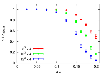
Figure 1: Left: the average sign, $\langle\varepsilon\rangle_{abs,\mu}$ for the 3 spatial volumes as a function of the chemical potential $\mu$. Right: the factor $f(\mu,V)$ parametrizing the average sign; see (10).

3.1 Monte-Carlo with $\mu>0$

We would like to generate configurations with the weight $|{\rm Re\,}{\rm det\,}D(U,\mu)|e^{-S_{g}(U)}$. This is a non-trivial problem and to our knowledge no pseudo-fermion type construction can be found. What one may still do is rewrite the weight as

$$|{\rm Re\,}{\rm det\,}D(U,\mu)|e^{-S_{g}(U)}=\frac{|{\rm Re\,}{\rm det\,}D(U,\mu)|}{|{\rm Re\,}{\rm det\,}D(U,0)|}{\rm det\,}D(U,0)e^{-S_{g}(U)}\;,$$ (7)

since ${\rm det\,}D(U,0)$ is real and positive, and utilize a standard (R)HMC algorithm at $\mu=0$ and include the $\mu$-dependent ratio in the Metropolis accept/reject step at the end of the trajectory. This will clearly be an expensive algorithm because the full determinant needs to be computed, but with the help of the reduced matrix construction the cost is still manageable for the lattice volumes we will consider in this paper.

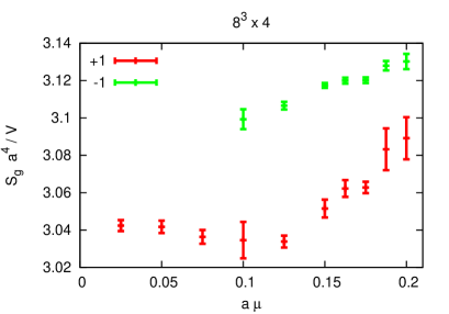
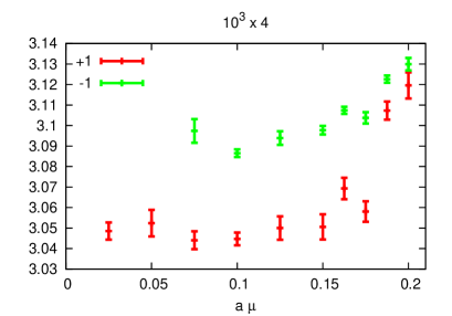
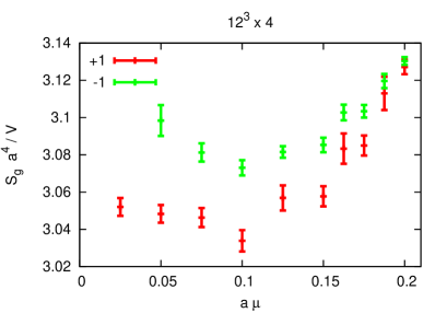
Figure 2: The gauge action per unit space time volume $S_{g}\;a^{4}/V=S_{g}\;(a/L)^{3}\;aT$ for the 3 spatial volumes and the sectors $+1$ and $-1$ separately. For the low chemical potentials there are no configurations within the sector $-1$ in our ensembles.

Since we are working with rooted staggered fermions we need to compute the full determinant, its square root, its real part and then its sign and absolute value. At finite temperature these steps can most easily be done with the help of the reduced matrix Hasenfratz:1991ax . This has $6(L/a)^{3}$ eigenvalues, $\lambda_{i}(U)$, and the main utility of them is that the full staggered determinant can be given at finite chemical potential as,

$${\rm det\,}D_{st}(U,\mu)=\prod_{i}\left(\lambda_{i}(U)e^{-\frac{\mu}{2T}}-e^{\frac{\mu}{2T}}\right)\;.$$ (8)

For the precise definition of the reduced matrix see Hasenfratz:1991ax . We will define the square root branch factor-by-factor in the above product by requiring continuity in $\mu$ or in other words by requiring that in the $\mu\to 0$ limit each factor below goes to unity,

$$\frac{{\rm det\,}D(U,\mu)}{{\rm det\,}D(U,0)}=\left(\frac{{\rm det\,}D_{st}(U,\mu)}{{\rm det\,}D_{st}(U,\mu)}\right)^{1/2}=\prod_{i}\left(\frac{\lambda_{i}(U)e^{-\frac{\mu}{2T}}-e^{\frac{\mu}{2T}}}{\lambda_{i}(U)-1}\right)^{1/2}\;.$$ (9)

The branch cut of the square root is placed on the negative real axis. This procedure fully fixes the complex determinant ratio. The real part, sign and absolute value can then be taken straightforwardly. Notice that with this procedure the partition function remains real since ${\rm det\,}D(U^{*},\mu)={\rm det\,}D(U,\mu)^{*}$ for real $\mu$, and so our approach maintains its validity.

Clearly, if $\mu$ is small the ratio $|{\rm Re\,}{\rm det\,}D(U,\mu)|/|{\rm Re\,}{\rm det\,}D(U,0)|$ is close to unity and hence will not affect the Metropolis step much, i.e., a tuned (R)HMC algorithm at $\mu=0$ will perform just as well. On a given spatial volume as $\mu$ increases the ratio will influence the Metropolis step more and more and will decrease the acceptance rate. This can be compensated by employing shorter (R)HMC trajectories as this will change the links less and consequently the change in the ratio with respect to the beginning and end of the trajectory will decrease. In this way we are able to keep the acceptance rate above $50\%$ for all runs. The shorter trajectories will of course lead to larger autocorrelation times. Concretely, our estimate of integrated autocorrelation times of our key observable (11) are between 50 and 500 depending on $\mu$ and $L/a$. The total number of configurations are between $5\cdot 10^{4}$ and $2\cdot 10^{5}$, leading to a few hundred independent configurations for each simulation point. We observe that “tunnelling” between the $+1$ and $-1$ sectors are frequent, i.e., the change in the $\mu$-dependent ratio is small enough so that even if the trajectory changes sector we observe good acceptance.

The crucial measure of whether the results are reliable or not is given by $\langle\varepsilon\rangle_{abs,\mu}$, i.e., the average sign, which at the same time measures the strength of the sign problem itself. Since $\langle\varepsilon\rangle_{abs,\mu}\to 1$ as $\mu\to 0$ we parametrize it as,

$$\langle\varepsilon\rangle_{abs,\mu}=e^{-V\mu^{2}f(\mu,V)}$$ (10)

with the 4-volume $V=L^{3}/T$ and show in figure 1 both $\langle\varepsilon\rangle_{abs,\mu}$ as well as $f(\mu,V)$. Clearly, $f(\mu,V)$ depends mildly on $V$ but does depend non-trivially on $\mu$. As can be seen the volumes $L/a=8,10,12$ and chemical potentials $a\mu\leq 0.2$ are safely in the region where $\langle\varepsilon\rangle_{abs,\mu}$ is several standard deviations away from zero, hence the sign reweighting (5) can be performed without issues. In particular, as emphasized, there is no overlap problem to contend with.

It is worth exploring what the effect of the sign reweighting is on some observables, more precisely how different some observables are in the $+1$ and $-1$ sectors. As an example we show the gauge action per unit space time volume in figure 2 as a function of the chemical potential separately for the two sectors.

3.2 Fisher zeros

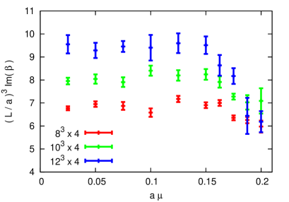
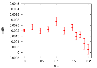
Figure 3: Left: the measured imaginary parts of the Fisher zeros scaled by the spatial volume. Right: the infinite volume extrapolated imaginary part of the Fisher zeros. The result at $\mu=0$ was obtained using the standard (R)HMC algorithm.

Once it has been determined which volumes and chemical potentials allow for the application of the sign reweighting (5) we are able to compute observables. Since our primary interest is the order of the phase transition as a function of $\mu$ we will compute the Fisher zeros in the bare coupling $\beta$, i.e., we will look for complex bare couplings such that $Z(\mu,\beta)=0$ at given $\mu$ and volume; see (2). This amounts to measuring the observables

$${\cal O}(U)=e^{-(\beta-\beta_{c})\frac{S_{g}(U)}{\beta_{c}}}$$ (11)

for complex $\beta$, assuming the simulation was done at (real) bare coupling $\beta_{c}$. Since ${\cal O}(U^{*})={\cal O}(U)$ our method can be applied without problems. More precisely, since $Z(\mu,\beta)$ has several zeros as a function of complex $\beta$, we will be looking for the one closest to the real axis, which in every run happens to coincide with the one closest to $(\beta_{c},0)$ in the complex plane as well. This zero will be called the leading zero.

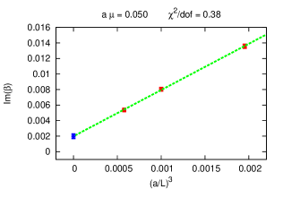
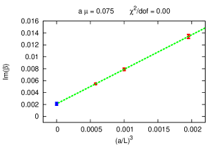
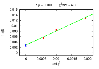
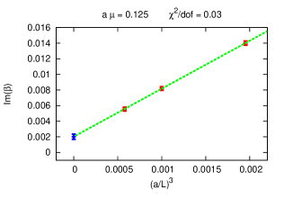
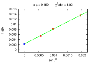
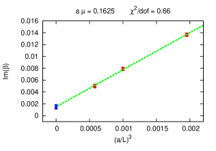
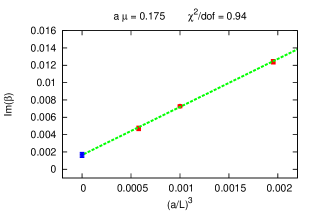
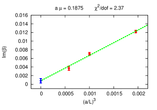
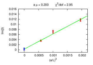
Figure 4: The infinite volume extrapolations (12) of the imaginary parts of the leading Fisher zeros at the various chemical potentials we have simulated at.

The volume scaling of ${\rm Im\,}\beta$ determines the order of the transition: if ${\rm Im\,}\beta\to const$ as $L/a\to\infty$ the transition is a cross-over, if ${\rm Im\,}\beta\sim a^{3}/L^{3}$ the transition is first order and finally if ${\rm Im\,}\beta\sim(a/L)^{\alpha}$ with a non-trivial exponent $\alpha>0$ the transition is second order. Although these leading order expressions are unambiguous in all three cases, the subleading terms are a priori not known. Since we know that at $\mu=0$ the transition is a cross-over for physical quark masses, it is generally expected that for small $\mu$ it will stay a cross-over. At fixed $\mu>0$ the imaginary part of the leading Fisher zero is then extrapolated to infinite volume via,

$${\rm Im\,}\beta = A+B\,(a/L)^{3}\;,$$ (12)

where the exponent $3$ in the subleading term is merely an ansatz. In this first study we only simulated at 3 volumes, $L/a=8,10,12$ and hence we are unable to fit the exponent of the subleading term simultaneously with $A$ and $B$. Empirically, we do find that the above fit function provides acceptable statistical fits for our choice of chemical potentials.

The existence of a critical end point would suggest that ${\rm Im\,}\beta_{\infty}(\mu)=A(\mu)$ is a decreasing function of $\mu$ and as $\mu\to\mu_{c}$ we have $A(\mu)\to 0$.

The real part of the leading Fisher zero on the other hand may be used to define the critical coupling. The simulations we performed at particular values of $\beta_{c}=\beta_{c}(\mu)$ and we have checked that for $a\mu>0.1$ the differences $\Delta\beta={\rm Re\,}\beta-\beta_{c}$ are deviating from zero less than $3\sigma$ and rarely beyond $1.5\sigma$. Note that a smooth cross-over means that different observables may lead to different definitions of the pseudo-critical coupling.

The measured imaginary parts of the Fisher zeros are shown in the left panel of figure 3. The extrapolations to infinite volume using $L/a=8,10,12$ are shown in figure 4 together with the resulting $\chi^{2}/dof$ values of the fits. Out of the 10 extrapolations the largest $\chi^{2}/dof$ values are at $a\mu=0.1,\;0.1875,\;0.2$ and are $4.3,\;2.37,\;2.95$. Note that $dof=1$ and even the largest $\chi^{2}/dof=4.3$ leads to a q-value of $4\%$. The resulting ${\rm Im\,}(\beta_{\infty}(\mu))$ as a function of $\mu$ is finally shown in the right panel of figure 3.

The most important result from our investigation can be gleaned from figure 3. Both at finite volumes and correspondingly in infinite volume the imaginary part of the relevant Fisher zero is decreasing as the chemical potential becomes sufficiently large. More precisely, the infinite volume extrapolated result shows that the imaginary part of the leading Fisher zero is more or less flat up to $a\mu\sim 0.15$ and a sharp decrease is observed for $0.15\leq a\mu\leq 0.2$. The observed flatness agrees within errors with the slight increase seen in Fodor:2004nz ; Giordano:2020uvk , and cannot be significantly distinguished from it with the currently available statistics. This means that in the range of chemical potentials where our results are reliable with trustworthy statistical errors, i.e., $\langle\varepsilon\rangle_{abs,\mu}\neq 0$, we are able to conclude with high statistical significance that the leading singularity of $\log Z$ is eventually moving closer and closer to the real axis. In fact, the location of the singularity is consistent with a real value at $a\mu\sim 0.2$. This in turn means that the strength of the transition is eventually increasing and very suggestive that a true phase transition occurs at around $a\mu\sim 0.2$. This corresponds to $\mu/T_{c}\sim 0.8$, in agreement with Fodor:2004nz , however the latter result should be interpreted with caution since, as we explained, we do not expect the fixed $N_{t}=4$ results to be particularly close to the continuum with our chosen discretization. Nonetheless our results are trustworthy in the well defined statistical model given by the $N_{t}=4$ lattice system.

4 Conclusion and outlook

In this paper we have introduced a new technique for evaluating the path integral at finite baryon chemical potential. The approach involves generating configurations by the absolute value of the real part of the fermionic determinant and taking the signs into account by a discrete reweighting. The first step necessitates the evaluation of the full determinant during the Monte-Carlo simulation which makes the algorithm rather costly but still manageable for $8^{3}\times 4$, $10^{3}\times 4$ and $12^{3}\times 4$ which are the volumes we used. The second step, the discrete reweighting by the sign of the real part of the fermionic determinant, is a fully controlled step provided the average sign is several standard deviations away from zero, i.e., the sign problem is not too severe. This requirement can be easily monitored and once it is fulfilled, the results are completely trustworthy with well-defined statistical errors. This feature is the main advantage of our method. It improves on traditional reweighting in $\mu$ and/or some other continuous parameter because in that case the notorious overlap problem may invalidate the results even though a naive application of the reweighting formula $\langle{\cal O}\rangle_{\mu}=\langle{\cal O}w\rangle_{0}/\langle w\rangle_{0}$ seemingly presents no problems.

Since our main interest was the order of the thermal phase transition as a function of the chemical potential, we have determined the first few Fisher zeros and the volume scaling of the leading one (the one closest to the real axis) for 10 choices of $\mu$ in the range $0.025\leq a\mu\leq 0.2$. We have observed that the strength of the phase transition stays flat within errors for $0<a\mu<0.15$ and increases sharply for $0.15<a\mu<0.2$, signified by the decrease in the imaginary part of the leading Fisher zero. The infinite volume extrapolation of the leading Fisher zero at $a\mu\sim 0.2$, corresponding to $\mu_{B}/T\sim 2.4$, is in fact consistent with a true phase transition, i.e., the imaginary part is consistent with zero.

There are however several avenues to improve on our work in the future. First, we have performed simulations at fixed $N_{t}=4$, i.e., we have not addressed the continuum limit at all; simulations with larger temporal extents would be necessary in order to do so. Once the continuum behavior is investigated it might be worthwhile to use an improved action, both for the gauge and fermionic actions. In the present work we have used the Wilson plaquette gauge action and unimproved staggered fermions. The motivation was to replicate the setup of Fodor:2004nz where the critical end point was investigated using traditional reweighting in $\mu$. It is worth noting that even though the unimproved staggered discretization on $N_{t}=4$ lattices is far from the continuum, it is a well-defined lattice statistical physics model with a sign problem. Hence it makes perfect sense to study it in order to gain valuable insight into the sign problem in general.

Second, the volume scaling of the Fisher zeros is of central importance and our ansatz (12) was simply motivated by empirically observing good statistical fits as well as the fact that we only had data on 3 volumes. Hence we were unable to fit all 3 parameters, $A,B$ and $C$ in the general form,

$${\rm Im\,}\beta=A+B\,(a/L)^{C}\;,$$ (13)

which would otherwise be the justified procedure. Once an additional volume $14^{3}\times 4$ is added, the exponent $C$ could be determined or at least constrained.

Third, we have set the quark masses to their physical values at $\beta=\beta_{c}$ at $\mu=0$ and have not changed them for $\mu>0$ along the line of constant physics. Even though the effect is expected to be negligible relative to other sources of errors, in future work we do plan to follow the line of constant physics for $\mu>0$.

Fourth, we have included the chemical potential at the quark level as $\mu_{u}=\mu_{d}=\mu_{B}/3=\mu$ and $\mu_{s}=0$ which corresponds to $\mu_{S}=\mu_{B}/3$. Nonetheless our method can be trivially modified to include other chemical potential assignments, e.g., strangeness neutrality $\langle S\rangle=0$ or $\mu_{S}=0$.

Finally we mention that the recently introduced geometric matching procedure Giordano:2019gev provides a new rooting procedure at finite $N_{t}$ which is nonetheless expected to agree with the one followed in this paper towards the continuum limit. We repeated the determination of the leading Fisher zeros using geometric matching and found that they agree with the ones presented in this paper within statistical uncertainties. This type of cross-check will be especially useful for future studies targeting the continuum limit.

References

- (1) C. R. Allton, S. Ejiri, S. J. Hands, O. Kaczmarek, F. Karsch, E. Laermann, C. Schmidt and L. Scorzato, Phys. Rev. D 66, 074507 (2002) [hep-lat/0204010].
- (2) R. V. Gavai and S. Gupta, Phys. Rev. D 68, 034506 (2003) [arXiv:hep-lat/0303013 [hep-lat]].
- (3) R. Gavai and S. Gupta, Phys. Rev. D 71, 114014 (2005) [arXiv:hep-lat/0412035 [hep-lat]].
- (4) C. R. Allton, M. Doring, S. Ejiri, S. J. Hands, O. Kaczmarek, F. Karsch, E. Laermann and K. Redlich, Phys. Rev. D 71, 054508 (2005) [hep-lat/0501030].
- (5) R. V. Gavai and S. Gupta, Phys. Rev. D 78, 114503 (2008) [arXiv:0806.2233 [hep-lat]].
- (6) S. Basak et al. [MILC Collaboration], PoS LATTICE 2008, 171 (2008) [arXiv:0910.0276 [hep-lat]].
- (7) S. Borsanyi, Z. Fodor, S. D. Katz, S. Krieg, C. Ratti and K. Szabo, JHEP 1201, 138 (2012) [arXiv:1112.4416 [hep-lat]].
- (8) S. Borsanyi, G. Endrodi, Z. Fodor, S. D. Katz, S. Krieg, C. Ratti and K. K. Szabo, JHEP 1208, 053 (2012) [arXiv:1204.6710 [hep-lat]].
- (9) R. Bellwied, S. Borsanyi, Z. Fodor, S. D. Katz, A. Pasztor, C. Ratti and K. K. Szabo, Phys. Rev. D 92, no. 11, 114505 (2015) [arXiv:1507.04627 [hep-lat]].
- (10) H.-T. Ding, S. Mukherjee, H. Ohno, P. Petreczky and H.-P. Schadler, Phys. Rev. D 92, no. 7, 074043 (2015) [arXiv:1507.06637 [hep-lat]].
- (11) A. Bazavov et al., Phys. Rev. D 95, no. 5, 054504 (2017) [arXiv:1701.04325 [hep-lat]].
- (12) A. Bazavov et al. [HotQCD Collaboration], Phys. Lett. B 795, 15 (2019) [arXiv:1812.08235 [hep-lat]].
- (13) M. Giordano and A. Pasztor, Phys. Rev. D 99, no. 11, 114510 (2019) [arXiv:1904.01974 [hep-lat]].
- (14) A. Bazavov et al., arXiv:2001.08530 [hep-lat].
- (15) P. de Forcrand and O. Philipsen, Nucl. Phys. B 642, 290 (2002) [hep-lat/0205016].
- (16) M. D’Elia and M. P. Lombardo, Phys. Rev. D 67, 014505 (2003) [hep-lat/0209146].
- (17) M. D’Elia and F. Sanfilippo, Phys. Rev. D 80, 014502 (2009) [arXiv:0904.1400 [hep-lat]].
- (18) P. Cea, L. Cosmai and A. Papa, Phys. Rev. D 89, no. 7, 074512 (2014) [arXiv:1403.0821 [hep-lat]].
- (19) C. Bonati, P. de Forcrand, M. D’Elia, O. Philipsen and F. Sanfilippo, Phys. Rev. D 90, no. 7, 074030 (2014) [arXiv:1408.5086 [hep-lat]].
- (20) P. Cea, L. Cosmai and A. Papa, Phys. Rev. D 93, no. 1, 014507 (2016) [arXiv:1508.07599 [hep-lat]].
- (21) C. Bonati, M. D’Elia, M. Mariti, M. Mesiti, F. Negro and F. Sanfilippo, Phys. Rev. D 92, no. 5, 054503 (2015) [arXiv:1507.03571 [hep-lat]].
- (22) R. Bellwied, S. Borsanyi, Z. Fodor, J. Gunther, S. D. Katz, C. Ratti and K. K. Szabo, Phys. Lett. B 751, 559 (2015) [arXiv:1507.07510 [hep-lat]].
- (23) M. D’Elia, G. Gagliardi and F. Sanfilippo, Phys. Rev. D 95, no. 9, 094503 (2017) [arXiv:1611.08285 [hep-lat]].
- (24) J. N. Guenther, R. Bellwied, S. Borsanyi, Z. Fodor, S. D. Katz, A. Pasztor, C. Ratti and K. K. Szabó, Nucl. Phys. A 967, 720 (2017) [arXiv:1607.02493 [hep-lat]].
- (25) P. Alba et al., Phys. Rev. D 96, no. 3, 034517 (2017) [arXiv:1702.01113 [hep-lat]].
- (26) V. Vovchenko, A. Pasztor, Z. Fodor, S. D. Katz and H. Stoecker, Phys. Lett. B 775, 71 (2017) [arXiv:1708.02852 [hep-ph]].
- (27) C. Bonati, M. D’Elia, F. Negro, F. Sanfilippo and K. Zambello, Phys. Rev. D 98, no. 5, 054510 (2018) [arXiv:1805.02960 [hep-lat]].
- (28) S. Borsanyi, Z. Fodor, J. N. Guenther, S. K. Katz, K. K. Szabo, A. Pasztor, I. Portillo and C. Ratti, JHEP 1810, 205 (2018) [arXiv:1805.04445 [hep-lat]].
- (29) R. Bellwied et al., Phys. Rev. D 101, no. 3, 034506 (2020) [arXiv:1910.14592 [hep-lat]].
- (30) S. Borsanyi et al., arXiv:2002.02821 [hep-lat].
- (31) E. Seiler, D. Sexty and I. O. Stamatescu, Phys. Lett. B 723, 213 (2013) [arXiv:1211.3709 [hep-lat]].
- (32) D. Sexty, Phys. Lett. B 729, 108 (2014) [arXiv:1307.7748 [hep-lat]].
- (33) G. Aarts, E. Seiler, D. Sexty and I. O. Stamatescu, Phys. Rev. D 90, no. 11, 114505 (2014) [arXiv:1408.3770 [hep-lat]].
- (34) Z. Fodor, S. D. Katz, D. Sexty and C. Torok, Phys. Rev. D 92, no. 9, 094516 (2015) [arXiv:1508.05260 [hep-lat]].
- (35) D. Sexty, Phys. Rev. D 100, no. 7, 074503 (2019) [arXiv:1907.08712 [hep-lat]].
- (36) J. B. Kogut and D. K. Sinclair, Phys. Rev. D 100, no. 5, 054512 (2019) [arXiv:1903.02622 [hep-lat]].
- (37) M. Scherzer, D. Sexty and I. Stamatescu, [arXiv:2004.05372 [hep-lat]].
- (38) A. Hasenfratz and D. Toussaint, Nucl. Phys. B 371, 539 (1992).
- (39) I. M. Barbour, S. E. Morrison, E. G. Klepfish, J. B. Kogut and M. P. Lombardo, Nucl. Phys. Proc. Suppl. 60A, 220 (1998) [hep-lat/9705042].
- (40) Z. Fodor and S. D. Katz, Phys. Lett. B 534, 87 (2002) [hep-lat/0104001].
- (41) Z. Fodor and S. D. Katz, JHEP 0203, 014 (2002) [hep-lat/0106002].
- (42) Z. Fodor and S. D. Katz, JHEP 0404, 050 (2004) [hep-lat/0402006].
- (43) M. Giordano, K. Kapas, S. D. Katz, D. Nogradi and A. Pasztor, arXiv:1911.00043 [hep-lat].
- (44) M. Cristoforetti et al. [AuroraScience], Phys. Rev. D 86, 074506 (2012) [arXiv:1205.3996 [hep-lat]].
- (45) M. Cristoforetti, F. Di Renzo, A. Mukherjee and L. Scorzato, Phys. Rev. D 88 (2013) no.5, 051501 [arXiv:1303.7204 [hep-lat]].
- (46) A. Alexandru, G. Basar and P. Bedaque, Phys. Rev. D 93, no. 1, 014504 (2016) [arXiv:1510.03258 [hep-lat]].
- (47) A. Alexandru, G. Basar, P. F. Bedaque, G. W. Ridgway and N. C. Warrington, Phys. Rev. D 93, no. 9, 094514 (2016) [arXiv:1604.00956 [hep-lat]].
- (48) J. Nishimura and S. Shimasaki, JHEP 1706, 023 (2017) [arXiv:1703.09409 [hep-lat]].
- (49) C. Gattringer, PoS LATTICE 2013, 002 (2014) [arXiv:1401.7788 [hep-lat]].
- (50) C. Marchis and C. Gattringer, Phys. Rev. D 97, no. 3, 034508 (2018) [arXiv:1712.07546 [hep-lat]].
- (51) G. Aarts, E. Seiler and I. O. Stamatescu, Phys. Rev. D 81, 054508 (2010) [arXiv:0912.3360 [hep-lat]].
- (52) G. Aarts, F. A. James, E. Seiler and I. O. Stamatescu, Eur. Phys. J. C 71, 1756 (2011) [arXiv:1101.3270 [hep-lat]].
- (53) P. de Forcrand, S. Kim and T. Takaishi, Nucl. Phys. Proc. Suppl. 119, 541 (2003) [hep-lat/0209126].
- (54) P. de Forcrand, PoS LAT 2009, 010 (2009) [arXiv:1005.0539 [hep-lat]].
- (55) S. D. H. Hsu and D. Reeb, Int. J. Mod. Phys. A 25, 53 (2010).
- (56) A. Alexandru, M. Faber, I. Horvath and K. F. Liu, Phys. Rev. D 72, 114513 (2005) [hep-lat/0507020].
- (57) A. Li, A. Alexandru, K. F. Liu and X. Meng, Phys. Rev. D 82, 054502 (2010) [arXiv:1005.4158 [hep-lat]].
- (58) A. Li, A. Alexandru and K. F. Liu, Phys. Rev. D 84, 071503 (2011) [arXiv:1103.3045 [hep-ph]].
- (59) M. Giordano, K. Kapas, S. D. Katz, D. Nogradi and A. Pasztor, arXiv:2003.04355 [hep-lat].