Bayesian Nonparametric Modeling for Predicting Dynamic Dependencies in Multiple Object Trackings

Abstract

Some challenging problems in tracking multiple objects include the time dependent cardinality, unordered measurements and object parameter labeling. In this paper, we employ Bayesian Bayesian nonparametric methods to address these challenges. In particular, we propose modeling the multiple object parameter state prior using the dependent Dirichlet and Pitman-Yor processes. These nonparametric models have been shown to be more flexible and robust, when compared to existing methods, for estimating the time-varying number of objects, providing object labeling and identifying measurement to object associations. Monte Carlo sampling methods are then proposed to efficiently learn trajectory of objects from noisy measurements. Using simulations, we demonstrate the estimation performance advantage of the new methods when compared to existing algorithms such as the generalized labeled multi-Bernoulli filter.

Keywords: Bayesian nonparametric models, dependent Dirichlet process, dependent Pitman-Yor process, multiple object tracking, Markov chain Monte Carlo sampling

1 Introduction

Multiple object tracking under time-varying (TV) conditions is a challenging and computationally intensive problem Bar-Shalom (1990); Mahler (2007); Wang et al. (2017). It entails the estimation of a TV and unknown number of objects at each time step, using measurements with no known association to the objects. Some recent methods to solving this problem involve random finite set (RFS) theory methods, together with probability hypothesis density filtering and multi-Bernoulli filtering Vo et al. (2014); Reuter et al. (2014); Vo et al. (2015, 2017). Many methods cluster objects to their associated estimated state after tracking. The labeled multi-Bernoulli filter, on the other hand, uses labeled RFS to estimate the objects identity, although at a high computational cost and requiring high signal-to-noise ratios Vo et al. (2014); Reuter et al. (2014). In Aoki et al. (2016), maximum a posteriori estimates of object label uncertainties are integrated with a multiple hypothesis tracking algorithm.

In recent years, the ubiquitous influence of Bayesian nonparametric models has been well-established as a way to avoid the restrictions of parametric models. Infinite dimensional random measures, such as the Dirichlet process (DP) Ferguson (1973); Teh (2011) and Pitman-Yor process (PYP) Pitman and Yor (1997); Pitman (2002) have replaced finite mixture models for clustering, estimation and inference Antoniak (1974); Pitman (2002); Pitman and Yor (1997). Pólya urn approaches for TV DP and PYP mixtures have been used as priors on parameters over observations. Note, however, that they do not capture the full dependency in a problem and their marginal distributions are not well-defined Ahmed and Xing (2008); Blei and Frazier (2011); Caron et al. (2007, 2017); Moraffah et al. (2019b, a, c). A process that does describe dependency among collections of stochastic processes is the dependent DP and mixture models that can be used for clustering batch-sequential data with a TV number of clusters MacEachern (1999, 2000); Campbell et al. (2013); Neiswanger et al. (2014); Topkaya et al. (2013); Moraffah and Papandreou-Suppappola (2019, 2018); Moraffah (2019b).

In this paper, we propose a family of prior distributions for time-dependent tracking algorithms constructed using the dependent DP and PYP. A Markov chain Monte Carlo (MCMC) inferential method integrates the distributions to update the time dependent states. Our proposed methods outperform existing ones and are computationally efficient. We also show that they have well-defined marginal distributions and hence provide an efficient way to perform inference. They can capture the full time-dependency among object states and can represent objects entering and leaving a scene, label object states and accurately estimate object cardinality and trajectory. They are also simple to integrate with MCMC sampling methods for robust inference.

The rest of the paper is organized as follows. Section 2 summarizes the TV tracking formulation and Section 3 reviews the DP and PYP. In Section 4, we present the dependent DP prior, develop an MCMC inference method, and discuss algorithm convergence and properties. The extension to the dependent PYP as a prior and its advantages over the DP are provided in Section 5. Using simulations in Section 6, we demonstrate the methods’ improved performance when compared the RFS-based label multi-Bernoulli filter.

2 Multiple Object Tracking Formulation

We consider the problem of tracking an unknown and TV number of objects $N_{k}$ at time step $k$. The unknown state vector of the $\ell$th object, $\ell$ = $1,\ldots,N_{k}$, is denoted by $\mathbf{x}_{\ell,k}$. If the $\ell$th object is present at time step $(k-1)$ and transitions to time step $k$, then the object state follows $\mathbf{x}_{\ell,k}$ = $F(\mathbf{x}_{\ell,k-1})+\mathbf{u}_{\ell,k-1}$, where $F(\cdot)$ is a transition function and $\mathbf{u}_{\ell,k-1}$ is a modeling error random process. The problem is further complicated by the TV number of measurements $M_{k}$ and the unknown object association to a given measurement vector $\mathbf{z}_{m,k}$, $m$ = $1,\ldots,M_{k}$. We assume that each measurement is generated by only one object and that the measurements are independent of one another. If it is determined that the $m$th measurement originated from the $\ell$th object, the measurement equation for tracking is given by $\mathbf{z}_{m,k}$ = $R(\mathbf{x}_{\ell,k})+\mathbf{w}_{k}$; here, $R(\cdot)$ is a physics-based model describing the relation between the measurement to object state, and $\mathbf{w}_{k}$ is the measurement noise random process. Due to the large number of unknowns in the problem, additional functionality must be introduced. Whereas RFS theory was used in previous studies, we incorporate nonparametric methods, as will be demonstrated.

3 Nonparametric Random Processes as Priors

Dirichlet Process.  The DP model defines a prior on the space of probability distributions Ferguson (1973); Teh (2011). A DP, $G$$\sim$$\text{DP}(\alpha,H)$, on an infinite dimensional space with parameter set $\Theta$, concentration parameter $\alpha$, and base distribution $H$, is defined as

$$G(\theta)=\sum_{\ell=1}^{\infty}\pi_{\ell}\,\delta(\theta_{\ell}-\theta),\ \theta_{\ell}\sim H,\ \pi_{j}\sim\text{GEM}(\alpha)$$ (1)

where $\text{GEM}(\alpha)$ follows the stick breaking representation Sethuraman (1994)

$$\pi_{\ell}=V_{\ell}\prod_{l=1}^{\ell-1}(1-V_{l}),\ \text{where}\ V_{\ell}\sim\text{Beta}(1,\alpha),\ \ j=1,2,\ldots$$

and $\delta(\theta_{\ell}-\theta)$ = $1$ if $\theta$ = $\theta_{\ell}$, $\theta_{\ell}\!\!\in\!\!\Theta$, and zero otherwise. $G(\theta)$ is a discrete probability random measure with probability one. The DP mixture (DPM) model for parameters $y_{n}$, $n$ = $1,\ldots,N$, is $y_{n}\!\mid\!\theta_{n}\!\sim\!f(\cdot\mid\theta_{n})$, where $\theta_{n}\!\mid\!G\!\sim\!G$ and $G\!\mid\!\alpha,H\!\sim\!\text{DP}(\alpha,H)$. The independent and identically distributed parameters are drawn from $F(\cdot)$ = $\int_{\theta}f(\cdot\!\mid\!\theta)\,dG(\theta)$, where $f(\cdot$$\mid$$\theta)$ is the density and $G(\theta)$ is the mixing distribution drawn according to a DP in (1). It can be shown that the expected number of clusters using the DP model varies exponentially as $\alpha\log N$.

Pitman-Yor Process.  The PYP forms a large class of distributions on random probability measures that contains DPs; it is a subclass of $d$-Gibbs processes and shares the DP essential properties. Similar to the DP, it defines a prior on the space of probability distributions over the infinite dimension space of parameters. A PYP, $G$$\sim$$\text{PYP}(d,\alpha,H)$, has discount parameter $d$, $0\!\leq\!d\!<\!1$, concentration parameter $\alpha$, $\alpha\!>\!-d$, and base distribution $H$. When $d$ = $0$, the PYP simplifies to $\text{DP}(\alpha,H)$. A PYP realization is a discrete random measure that can be constructed using the stick breaking representation

$$G(\theta)=\sum_{\ell=1}^{\infty}\pi^{*}_{\ell}\,\delta(\theta_{\ell}-\theta),\ \theta_{\ell}\sim H$$ (2)

Here, $\pi^{*}_{\ell}$ is the size-biased order of $\pi_{\ell}$, $\pi_{\ell}$ = $V_{\ell}\prod_{l=1}^{\ell-1}(1-V_{l})$, and $V_{\ell}\sim\text{Beta}(1-d,\alpha+\ell\,d)$. Similar to the DPM, the PYP mixture model for $y_{n}$, $n$ = $1,\ldots,N$, is $y_{n}\!\mid\!\theta_{n}\!\sim\!f(\cdot\mid\theta_{n})$, $\theta_{n}\!\mid\!G\!\sim G$, and $G\!\mid\!\alpha,H\!\sim\!\text{PYP}(d,\alpha,H)$. The PYP expected number of clusters follows the power-law $\alpha N^{d}$ Teh (2006).

4 Tracking with Dependent Dirichlet Process

In order to capture the time-dependent evolution in multiple object tracking, we exploit the dependent DP (DDP) MacEachern (1999). The proposed DDP evolutionary Markov model (DDP-EMM) approach is used to learn multiple object attributes over related information. This information is based on dynamic dependencies in the state transition formulation. In particular, the number of objects at time step $k$ depends on the number of objects present at the previous time step $(k\!-\!1)$and on the objects popularity. Also, the clustering index of the $\ell$th object state at time step $k$ depends on the clustering index of the previous $(\ell\!-\!1)$ object states at the same time step.

4.1 Construction of DDP Evolutionary Markov Model

The DDP based construction of the prior distributions of the multiple object states follows three time evolution steps. Specifically, information from time step $(k\!-\!1)$ and from transitioning between time steps $(k\!-\!1)$ and $k$ is used to predict information at time step $k$. To aid in the construction and dynamically track relevant assignments in relation to the $\ell$th object and $l$th cluster at time step $k$, we define three indicators: cluster assignment $c_{l,k}$, object transitioning $\text{s}_{\ell,k}$, and cluster transitioning $\lambda_{l,k}$. The three-step construction is detailed next and summarized in Algorithm 1, and a graphical model of the evolutionary dependence is shown in Figure 1.

Figure 1: Graphical model capturing temporal dependence.

Step 1.  Previous time step:

At time step $(k\!-\!1)$, the parameter sets

$${\cal X}_{N_{k-1},k-1}=\{\mathbf{x}_{1,k-1},\ldots,\mathbf{x}_{N_{k-1},k-1}\}$$

and

$$\Theta_{N_{k-1},k-1}=\{\boldsymbol{\theta}_{1,k-1},\ldots,\boldsymbol{\theta}_{N_{k-1},k-1}\}$$

are assumed available. Here, the vectors $\mathbf{x}_{\ell,k-1}$ and $\boldsymbol{\theta}_{\ell,k-1}$ denote the $\ell$th object state and the cluster parameter associated with the $\ell$th object, $\ell$ = $1,\ldots,N_{k-1}$, respectively. To reduce computation, only $D_{k-1}\!\!\leq\!\!N_{k-1}$ non-empty clusters are considered with unique parameters $\Theta^{\star}_{D_{k-1},k-1}\!\!\subseteq\!\!\Theta_{N_{k-1},k-1}$. It is also assumed that the cardinality of the $l$th cluster (number of objects in the cluster) is $v^{\star}_{l,k-1}$ and its induced cluster assignment indicator is $c_{l,k-1}\!\in\!\{1,\ldots,D_{k-1}\}$. The set of induced cluster assignment indicators is denoted by $\mathcal{C}_{D_{k-1},k-1}$ = $\{c_{1,k-1},\ldots,c_{D_{k-1},k-1}\}$.

Step 2.  Transitioning between time steps.

From time steps $(k\!-\!1)$ to $k$, the binary object transitioning indicator $\text{s}_{\ell,k\mid k-1}$ determines the survival of the $\ell$th object. The indicators follow a Bernoulli process, with parameter $\text{P}_{\ell,k\mid k-1}$, associated with object transitioning. If $\text{s}_{\ell,k\mid k-1}$ = $1$, the object with state $\mathbf{x}_{\ell,k-1}$ transitions to time $k$ with probability $\text{P}_{\ell,k\mid k-1}$ according to the Markov transition kernel $F_{\boldsymbol{\theta}}(\mathbf{x}_{\ell,k-1},\cdot)$. If $\text{s}_{\ell,k\mid k-1}$ = $0$, the object leaves the scene with probability $(1-\text{P}_{\ell,k\mid k-1})$.

An empty cluster is assumed to no longer exist. Thus, the binary cluster transitioning indicator $\lambda_{l,k\mid k-1}$ is defined to keep track of the number of transitioning clusters $D_{k\mid k-1}$. Specifically, if the $l$th cluster cardinality satisfies $v^{\star}_{l,k-1}\!\!\geq\!\!1$, $\lambda_{l,k\mid k-1}$ = $1$; otherwise, $\lambda_{l,k\mid k-1}$ = $0$, $l$ = $1,\ldots,D_{k-1}$ and $D_{k\mid k-1}$ = $\sum_{l=1}^{D_{k-1}}\lambda_{l,k\mid k-1}$. The $l$th transitioning cluster cardinality is set to $v^{\star}_{l,k\mid k-1}$, and the parameter of the transitioning cluster associated with the $\ell$th object is $\boldsymbol{\theta}^{\star}_{\ell,k\mid k-1}$.

Step 3.  Current time step.

The three cases discussed next are used to formulate the distributions of both the DP cluster parameter $\boldsymbol{\theta}_{\ell,k}$ and its associated object state $\mathbf{x}_{\ell,k}$ at time step $k$. The number of non-empty clusters is set to $D_{k}$ = $D_{k\mid k-1}$, and the cardinality of the $l$th transitioning cluster is set to $v_{l,k}$ = $v^{\star}_{l,k\mid k-1}$, $l$ = $1,\ldots,D_{k}$.

Case D1: The $\ell$th transitioned object, with $\text{s}_{\ell,k\mid k-1}$ = $1$, is assigned to a transitioned cluster already occupied by at least one of the $(\ell\!-\!1)$ previous objects. As the cluster assignment set $\mathcal{C}_{D_{k},k}$ at time step $k$ induces an infinite exchangeable random partition, it is assumed that the $\ell$th object is the last to be clustered and selects one of these clusters with probability

$$\Pi^{(1)}_{k}=\text{Pr}\Big{(}\text{select}\ l\text{th}\ \text{cluster},l\!\leq\!D_{k}\mid\Theta_{\ell-1,k}\Big{)}$$

$$=\dfrac{1}{g_{k}}\Big{(}v_{l,k}+\sum_{j=1}^{D_{k-1}}v^{\star}_{j,k\mid k-1}\,\lambda_{j,k\mid k-1}\,\delta(c_{j,k}-c_{l,k})\Big{)},$$ (3)

$g_{k}$ = $(\ell-1)+\alpha+\sum_{l=1}^{\ell-1}\sum_{j=1}^{D_{k-1}}v^{\star}_{j,k\mid k-1}\lambda_{j,k\mid k-1}\delta(c_{j,k}-c_{l,k})$ and $\alpha$$>$$0$ is the concentration parameter. The cluster parameter $\boldsymbol{\theta}_{\ell,k}$ associated to the $\ell$th object is drawn from the transitioning kernel $\varphi(\boldsymbol{\theta}^{*}_{\ell,k-1},\boldsymbol{\theta}_{\ell,k})$. With probability $\Pi^{(1)}_{k}$, the $\ell$th object state prior distribution is drawn as

$$p_{1}\Big{(}\mathbf{x}_{\ell,k}\mid\Upsilon_{\ell,k}\Big{)}=F_{\boldsymbol{\theta}}(\mathbf{x}_{\ell,k-1},\mathbf{x}_{\ell,k})\;f(\mathbf{x}_{\ell,k}\mid\boldsymbol{\theta}^{*}_{\ell,k}),$$ (4)

where $F_{\boldsymbol{\theta}}(\mathbf{x}_{\ell,k-1},\cdot)$ is the object transitioning kernel and $f(\mathbf{x}_{\ell,k}\!\mid\!\!\cdot)$ is the object state density. The conditional parameter set in (4) is $\Upsilon_{\ell,k}$ = $\{{\cal X}_{\ell-1,k},{\cal X}_{\ell,k\mid k-1},\Theta_{\ell,k},\Theta^{*}_{\ell,k\mid k-1}\}$.

Case D2: The $\ell$th object is assigned to one of the transitioning clusters that has not yet been assigned to any of the $(\ell-1)$ previous objects. The object selects one of these clusters with probability

$$\Pi^{(2)}_{k}=\text{Pr}\big{(}\text{select}\ l\text{th}\ \text{cluster},\ l\leq D_{k}\,\mid\Theta_{\ell-1,k}\big{)}$$

$$\hskip 7.22743pt=\dfrac{1}{g_{k}}\Big{(}\sum_{j=1}^{D_{k-1}}\!\!v^{\star}_{j,k\mid k-1}\lambda_{j,k\mid k-1}\delta(c_{j,k}-c_{l,k})\Big{)}\,.$$ (5)

The cluster parameter $\boldsymbol{\theta}_{\ell,k}$ associated to the $\ell$th object is drawn from $\varphi(\boldsymbol{\theta}^{*}_{\ell,k-1},\boldsymbol{\theta}_{\ell,k})$. With probability $\Pi^{(2)}_{k}$, the state prior distribution is drawn as

$$p_{2}(\mathbf{x}_{\ell,k}\mid\Upsilon_{\ell,k})=F_{\boldsymbol{\theta}}(\mathbf{x}_{\ell,k-1},\mathbf{x}_{\ell,k})\,f(\mathbf{x}_{\ell,k}\mid\boldsymbol{\theta}^{*}_{\ell,k})$$

$$\hskip 72.26999pt\cdot\,\varphi(\boldsymbol{\theta}^{*}_{\ell,k-1},\boldsymbol{\theta}_{\ell,k-1})\,.$$ (6)

Case D3: The $\ell$th object does not belong to an existing cluster, and a new cluster is formed with associated parameter vector drawn from the base of DP$(\alpha,H)$, $\boldsymbol{\theta}_{\ell,k}\sim H$. The object is selects this cluster with probability

$$\Pi^{(3)}_{k}=\text{Pr}\big{(}\text{new cluster}\mid\Theta_{\ell-1,k}\big{)}=\alpha/g_{k}\,.$$ (7)

The state prior distribution is drawn as

$$p_{3}(\mathbf{x}_{\ell,k}\mid\Upsilon_{\ell,k})=\int_{\boldsymbol{\theta}}f(\mathbf{x}_{\ell,k}\mid\boldsymbol{\theta})\,dH(\boldsymbol{\theta})\,.$$ (8)

Assuming the space of state parameters is Polish, the DDP in Cases D1–D3 define marginal DPs at each time step $k$, given the DDP configurations at time step $(k-1)$. Specifically,

$$\text{DDP-EMM}_{k}|\text{DDP-EMM}_{k-1}\sim\text{DP}\Big{(}\alpha,H_{0}\Big{)}$$ (9)

with base distribution

$$H_{0}=\sum_{\begin{subarray}{c}j=1\\[0.56905pt] \boldsymbol{\theta}_{j,k}\in\Theta_{D_{k},k}\end{subarray}}^{D_{k}}\Pi^{(1)}_{k}\,\delta(\boldsymbol{\theta}_{j,k}-\boldsymbol{\theta}_{\ell,k})+\Pi^{(3)}_{k}\,H(\boldsymbol{\theta}_{\ell,k})$$

$$+\sum_{\begin{subarray}{c}j=1\\[2.84526pt] \boldsymbol{\theta}^{\star}_{j,k}\in\Theta^{\star}_{D_{k},k\mid k-1}\setminus\Theta_{D_{k},k}\end{subarray}}^{D_{k}}\Pi^{(2)}_{k}\,\varphi(\boldsymbol{\theta}^{\star}_{\ell,k-1},\boldsymbol{\theta}_{\ell,k})\,\delta(\boldsymbol{\theta}_{j,k}-\boldsymbol{\theta}_{l,k}).$$ (10)

This model also allows the variation and labeling of clusters as it is defined in the space of partitions.

   Step 1. At time $(k\!-\!1)$, parameters available from Step 1

  $\bullet$ Object state parameters set, ${\cal X}_{N_{k-1},k-1}$

  $\bullet$ Cluster parameters set, $\Theta_{N_{k-1},k-1}$

  $\bullet$ Non-empty cluster unique parameters set, $\Theta^{\star}_{D_{k-1},k-1}$

  $\bullet$ Cluster assignment indicator set, $\mathcal{C}_{D_{k-1},k-1}$

  $\bullet$ Cardinality of $l$th non-empty cluster, $v^{\star}_{l,k-1}$

  

   Step 2. Transitioning between time steps $(k$$-$$1)$ and $k$

   Draw $\text{s}_{\ell,k\mid k-1}$$\sim$$\text{Bernoulli}(\text{P}_{\ell,k\mid k-1})$, $\ell$th object transitioning indicator

   If $\text{s}_{\ell,k\mid k-1}$ = $1$, $\ell$th object survives with probability (w.pr.) $\text{P}_{\ell,k\mid k-1}$ and transitions with kernel $F_{\boldsymbol{\theta}}(\mathbf{x}_{\ell,k-1},\mathbf{x}_{\ell,k})$

   If $l$th cluster cardinality satisfies $v^{\star}_{l,k-1}\geq 1$, set $l$th cluster transitioning indicator to $\lambda_{l,k\mid k-1}$ = $1$, $l$ = $1,\ldots,D_{k-1}$

   Set $\#$ of transitioning clusters to $D_{k\mid k-1}$ = $\sum_{l}\lambda_{l,k\mid k-1}$

   Denote cardinality of $l$th transitioning cluster by $v^{\star}_{l,k\mid k-1}$

   Denote parameter vector of transitioning cluster associated with $\ell$th object by $\boldsymbol{\theta}^{\star}_{\ell,k\mid k-1}$

  

   Step 3. At time $k$

   Set $D_{k}$ = $D_{k\mid k-1}$

  for $\ell$ = $1$ to $D_{k}$ do

      Set $v_{\ell,k}$ = $v^{\star}_{\ell,k\mid k-1}$

     if $\ell\leq D_{k}$ $\ell$th cluster already selected then

         Draw $\boldsymbol{\theta}_{\ell,k}\sim\varphi(\boldsymbol{\theta}^{*}_{\ell,k-1},\boldsymbol{\theta}_{\ell,k})$ with

         Draw $\mathbf{x}_{\ell,k}$$\mid$$\boldsymbol{\theta}_{\ell,k}\!\sim\!p_{1}(\mathbf{x}_{\ell,k}\mid\!\cdot)$ in (4) with prob. $\Pi^{(1)}_{k}$ in (3)

     else if $\ell\leq D_{k}$ $\ell$th cluster not yet selected then

         Draw $\boldsymbol{\theta}_{\ell,k}\sim\varphi(\boldsymbol{\theta}^{*}_{\ell,k-1},\boldsymbol{\theta}_{\ell,k})$

         Draw $\mathbf{x}_{\ell,k}$$\mid$$\boldsymbol{\theta}_{\ell,k}\!\sim\!p_{2}(\mathbf{x}_{\ell,k}\mid\!\cdot)$ in (6) with prob. $\Pi^{(2)}_{k}$ in (5)

     else

         Draw $\boldsymbol{\theta}_{\ell,k}\sim H$ for new cluster associated with $\ell$th object

         Draw $\mathbf{x}_{\ell,k}$$\mid$$\boldsymbol{\theta}_{\ell,k}\!\sim\!p_{3}(\mathbf{x}_{\ell,k}\mid\!\cdot)$ in (8) with prob. $\Pi^{(3)}_{k}$ in (7)

     end if

  end for

  return   $\{\mathbf{x}_{1,k},\mathbf{x}_{2,k},\ldots,\ldots\}$, $\{\boldsymbol{\theta}_{1,k},\boldsymbol{\theta}_{2,k},\ldots,\ldots\}$

Algorithm 1 DDP-EMM construction of prior distribution

4.2 Learning Model

Considering the measurements $\mathcal{Z}_{k}$ = $\{\mathbf{z}_{1,k},\ldots,\mathbf{z}_{M_{k},k}\}$ at time step $k$, the modeled prior distribution is used with an MCMC method to perform inference. The measurements are assumed independent, each generated from one object, and unordered; the $m$th measurement is not necessarily associated to the $\ell$th object, $m\neq\ell$. The posterior distribution is used to estimate the objects states and find the time-dependent object cardinality. As the DDP is used to label the object states at time step $k$, DPMs are used to learn and assign each measurement to its associated object identity. The mixing measure is drawn from the DDP in Algorithm 1 to infer the likelihood distribution

$$\mathbf{z}_{m,k}\mid\boldsymbol{\theta}_{\ell,k},\mathbf{x}_{\ell,k}\sim R(\mathbf{z}_{m,k}\mid\boldsymbol{\theta}_{\ell,k},\mathbf{x}_{\ell,k})$$ (11)

where $R(\mathbf{z}_{m,k}\mid\boldsymbol{\theta}_{\ell,k},\mathbf{x}_{\ell,k})$ is a distribution that depends on the measurement likelihood function. Algorithm 2 summarizes the mixing process that associates measurements to objects.

The Bayesian posterior to estimate the target trajectories is efficiently implemented using a Gibbs sampler inference scheme. The scheme iterates between sampling the object states and the dynamic DDP parameters, and it is based on the discreetness of the DDP MacEachern (2000); MacEarchern (1998). The Bayesian posterior is

$$p(\mathbf{x}_{\ell,k}\mid\mathcal{Z}_{k})=\int P(\mathbf{x}_{\ell,k}\mid\mathcal{Z}_{k},\Theta_{D_{k},k})\,dG(\Theta_{D_{k},k}\mid\mathcal{Z}_{k})$$ (12)

where $G(\Theta_{D_{k},k}\!\!\mid\!\!\mathcal{Z}_{k})$ is the cluster parameter posterior distribution given the measurements. As direct computation of (12) is intensive Antoniak (1974), Gibbs sampling is used to predict $\mathbf{x}_{\ell,k}$ using $p(\mathbf{x}_{\ell,k}\!\!\mid\!\!\mathcal{Z}_{k},\Theta_{D_{k},k})$ = $p(\mathbf{x}_{\ell,k}\!\mid\!\Theta_{D_{k},k})$, which is evaluated as $p(\mathbf{x}_{\ell,k}\!\mid\!\Theta_{D_{k},k})$ = $\int p(\mathbf{x}_{\ell,k}\!\mid\!\boldsymbol{\theta}_{\ell,k})\,d\pi(\boldsymbol{\theta}_{\ell,k}\!\mid\!\Theta_{D_{k},k})$. Here, the posterior of $\boldsymbol{\theta}_{\ell,k}$ given the remaining parameters is

$$\pi(\boldsymbol{\theta}_{\ell,k}\mid\Theta_{D_{k},k})=\sum_{\begin{subarray}{c}j=1,j\neq\ell\\[2.84526pt] \boldsymbol{\theta}_{j,k}\in\Theta_{D_{k},k}\end{subarray}}^{D_{k}}\Pi^{(1)}_{k}\,\delta(\boldsymbol{\theta}_{\ell,k}-\boldsymbol{\theta}_{j,k})+\Pi^{(3)}_{k}\,H(\boldsymbol{\theta}_{\ell,k})$$

$$+\sum_{\begin{subarray}{c}j=1,j\neq\ell\\[2.84526pt] \boldsymbol{\theta}_{j,k}\in\Theta^{\star}_{D_{k\mid k-1},k\mid k-1}\setminus\Theta_{D_{k},k}\end{subarray}}^{D_{k\mid k-1}}\!\!\!\Pi^{(2)}_{k}\,\varphi(\boldsymbol{\theta}^{\star}_{\ell,k-1},\boldsymbol{\theta}_{\ell,k})\,\delta(\boldsymbol{\theta}_{j,k}-\boldsymbol{\theta}_{\ell,k}).$$ (13)

The distribution obtained by combining the prior with the likelihood is

$$\boldsymbol{\theta}_{\ell,k}\mid\Theta^{(\ell)}_{k},\mathcal{Z}_{k}\ \sim\ \sum_{j=1}^{D_{k}}\xi_{j,k}\,\delta(\boldsymbol{\theta}_{\ell,k}-\boldsymbol{\theta}_{j,k})$$

$$+\sum_{\begin{subarray}{c}j=1\\ j\notin\mathcal{C}_{D_{k},k}\end{subarray}}^{D_{k\mid k-1}}\beta_{j,k}\,R_{j,k}(\boldsymbol{\theta}_{\ell,k})+\gamma_{\ell,k}\,H_{\ell}(\boldsymbol{\theta}_{\ell,k}),$$ (14)

where $\Theta^{(\ell)}_{k}$ = $\{\boldsymbol{\theta}_{1,k},\boldsymbol{\theta}_{2,k},\ \ldots,\ \boldsymbol{\theta}_{\ell-1,k},\boldsymbol{\theta}_{\ell+1,k},\hfill\ldots,\boldsymbol{\theta}_{D_{k\mid k-1},k}\}$, $R_{j,k}(\boldsymbol{\theta}_{\ell,k})$ = $R(\mathbf{z}_{\ell,k}\mid\mathbf{x}_{j,k},\boldsymbol{\theta}_{j,k})$,

$$\xi_{j,k}=\frac{R_{j,k}(\boldsymbol{\theta}_{\ell,k})}{g_{k}}\Big{(}v_{j,k}+\!\!\displaystyle\sum_{i=1}^{D_{k|k-1}}\!\!v^{\star}_{i,k\mid k-1}\lambda_{i,k\mid k-1}\delta(c_{i,k}-c_{j,k})\Big{)}$$

$$\beta_{j,k}=\frac{1}{g_{k}}\sum_{\begin{subarray}{c}i=1\\ i\notin\mathcal{C}_{D_{k},k}\end{subarray}}^{D_{k\mid k-1}}v^{\star}_{j,k\mid k-1}\lambda_{j,k\mid k-1}$$

$$\gamma_{\ell,k}=1-\sum_{j=1}^{D_{k}}\zeta_{j,k}-\sum_{\begin{subarray}{c}j=1\\ j\notin\mathcal{C}_{D_{k},k}\end{subarray}}^{D_{k\mid k-1}}\beta_{j,k}.$$

Also, $dH_{\ell}(\boldsymbol{\theta}_{\ell,k})\!\propto\!R_{j,k}(\boldsymbol{\theta}_{\ell,k})\,dH(\boldsymbol{\theta}_{\ell,k})$, $H$ is the base distribution on $\boldsymbol{\theta}_{\ell,k}$, and $g_{k}$ is defined below (3). The derivation is provided in Moraffah (2019a).

Algorithm 2 Infinite mixture model for measurement-to-object association

  Input: $\{\mathbf{z}_{1,k},\ldots,\mathbf{z}_{M_{k},k}\}$, measurements

  From construction of prior distribution from Algorithm 1

  Input: Object state vectors $\{\mathbf{x}_{1,k},\mathbf{x}_{2,k},\ldots\}$

  Input: Cluster parameter vectors $\{\boldsymbol{\theta}_{1,k},\boldsymbol{\theta}_{2,k},\ldots\}$

  Input: Cluster assignments ${\cal C}{\cal A}_{k-1}$ = $\{\mathcal{C}_{D_{k},1},\ldots,\mathcal{C}_{D_{k},k-1}\}$

   At time $k$:

  for $m$ = $1$ to $M_{k}$ do

     Draw $\mathbf{z}_{m,k}\mid\mathbf{x}_{\ell,k},\boldsymbol{\theta}_{\ell,k}$ from Equation (11)

     return  ${\cal C}_{D_{k},k}$, induced cluster assignment indicators

  end for

  Update: ${\cal C}{\cal A}_{k}$ = ${\cal C}{\cal A}_{k-1}\cup{\cal C}_{N_{k}}$

  return  $D_{k}$ (number of clusters) and ${\cal C}{\cal A}_{k}$

  return  posterior of $\mathbf{z}_{m,k}\mid\mathbf{x}_{\ell,k},\boldsymbol{\theta}_{\ell,k}$, $m$ = $1,\ldots,M_{k}$

4.3 DDP-EMM Approach Properties

Convergence

In the Gibbs sampler, it can be shown that the transition kernel converges to the posterior distribution for almost all initial conditions. If after $n$ iterations of the algorithm, $\Psi^{(n)}_{k}(\boldsymbol{\theta}_{\ell,0},\Theta_{D_{k},k})$ is the transition kernel for the Markov chain starting at $\boldsymbol{\theta}_{\ell,0}$ and stopping in the set $\Theta_{D_{k},k}$, then it can be shown to converge to the posterior $G(\Theta_{D_{k},k}\!\mid\!\mathcal{Z}_{k})$ given the measurements $\mathcal{Z}_{k}$ at time step $k$. Specifically,

$$||\Psi^{(n)}_{k}(\boldsymbol{\theta}_{\ell,0},\cdot)-G(\cdot\!\mid\!\mathcal{Z}_{k})||_{\text{TVN}}\rightarrow 0\ \text{as}\ n\rightarrow\infty,$$

for almost all initial conditions $\boldsymbol{\theta}_{\ell,0}$ in the total variation norm (TVN) (see Escobar and West (1995); Escobar (1994) in relation to the Gaussian distribution). The proof of convergence can be found in Moraffah (2019a).

Exchangeability

The infinite exchangeable random partition induced by $\mathcal{C}_{D_{k},k}$ at time $k$ follows the exchangeable partition probability function (EPPF) Aldous (1985)

$$p(\mathcal{V}^{\star}_{D_{k},k})=\frac{\alpha^{D_{k}}}{\alpha^{\left[N_{k}\right]}}\prod_{j=1}^{D_{k}}(v^{\star}_{j,k}-1)$$ (15)

where $\mathcal{V}^{\star}_{D_{k},k}$ = $\{v^{\star}_{1,k},\ \ldots,\ v^{\star}_{D_{k},k}\}$, $v^{\star}_{j,k}$ is the cardinality of the cluster with assignment indicator $c_{j,k}\in\mathcal{C}_{D_{k},k}$, $\alpha^{\left[n\right]}$ = $\alpha(\alpha+1)\dots(\alpha+n-1)$, and $D_{k}$ is the number of unique cluster parameters. Due to the variability of $N_{k}$, there is an important relationship between the partitions based on $N_{k}-1$ and $N_{k}$. In particular, the EPPF in (15) based on the partitions on $N_{k}$ and $N_{k}-1$ objects, given the configuration at time $(k-1)$, satisfies

$$p_{N_{k}-1}(\mathcal{V}^{\star}_{D_{k},k})=\sum_{j=1}^{D_{k}}p_{N_{k}}(\mathcal{V}^{\star}_{j,k})+p_{N_{k}}\big{(}\{\mathcal{V}^{\star}_{D_{k},k},1\}\big{)}$$ (16)

where $\mathcal{V}^{\star}_{j,k}$ = $\{v^{\star}_{1,k},\ \ldots,\ (v^{\star}_{j,k}+1),v^{\star}_{j+1,k},\ldots,\ v^{\star}_{D_{k},k}\}$. Equation (16) entails a notion of consistency of the partitions in the distribution sense. The equation holds due to the Markov property of the process given the configuration at time $(k-1)$.

Consistency

We consider $r_{\boldsymbol{\theta}_{0}}$ to be the true density of observations with probability measure $R_{\boldsymbol{\theta}_{0}}$. Then, if $r_{\boldsymbol{\theta}_{0}}$ is in the Kullback-Leibler (KL) support of the prior distribution in the space of all parameters Choi1and and Ramamoorthi (2008), then the posterior distribution $G(\cdot\!\mid\!\mathcal{Z}_{k})$ can be shown to be weakly consistent at $r_{\boldsymbol{\theta}_{0}}$ It is also important to investigate the posterior contraction rate as it is highly related to posterior consistency. This rate shows how fast the posterior distribution approaches the true parameters from which the measurements are generated. As detailed in Moraffah (2019a), the contraction rate matches the minimax rate for density estimators. Hence, the DDP prior constructed through the proposed model achieves the optimal frequentist rate.

5 Tracking with Dependent Pitman-Yor Process

Whereas the expected number of unique clusters used by the DP model during transitioning is $\alpha\log{(N_{k}})$, the number used by the PYP model follows the power law $\alpha N_{k}^{d}$. Here, $N_{k}$ is the number of objects to be clustered, $\alpha$ is a concentration parameter and $d$ is a discount parameter. With this additional parameter, the PYP model has a higher probability of having a large number of unique clusters Teh (2006). Also, clusters with only a small number of objects have a lower probability of selecting new objects. This more flexible model is better matched to tracking a TV number of objects as the larger number of available clusters ensures all dependencies are captured. The proposed dependent PYP (DPYP) state transitioning prior (DPYP-STP) method is presented next.

Construction Model  The construction of the DPYP prior distribution follows Steps 1 and 2 for the DDP in Section 4.1. As in Step 3 for the DDP, it is assumed that there are $D_{k}$ = $D_{k\mid k-1}$ non-empty clusters at time step $k$, and that the cardinality of the $l$th transitioning cluster is set to $v^{\star}_{l,k\mid k-1}$ = $v_{l,k}$, $l$ = $1,\ldots,D_{k}$. The state prior distributions are drawn following Cases D1-D3. However, the probability of an object selecting a particular cluster varies, as provided next in Cases P1–P3.

Case P1: The $\ell$th object is assigned, with probability

$$\Pi^{(1)}_{k}=\text{Pr}\Big{(}\text{select}\ l\text{th}\ \text{cluster},l\!\leq\!D_{k}\mid\Theta_{\ell-1,k}\Big{)}$$

$$=\dfrac{1}{g_{k}}\Big{(}v_{\ell,k}-d+\!\!\sum_{j=1}^{D_{k-1}}\!\!\!v^{\star}_{j,k\mid k-1}\,\lambda_{j,k\mid k-1}\,\delta(c_{j,k}-c_{\ell,k})\Big{)}$$ (17)

to a transitioning cluster that is already occupied by at least one of the $(\ell\!-\!1)$ previously transitioned objects. In (17), $g_{k}$ = $b_{\ell-1}+\alpha+\sum_{l=1}^{\ell-1}\sum_{j=1}^{D_{k-1}}v^{\star}_{j,k\mid k-1}\lambda_{j,k\mid k-1}\delta(c_{j,k}-c_{l,k})$, $b_{\ell-1}$ = $\sum_{j}^{\ell-1}v_{j,k}$, $\alpha\!\!>\!\!-d$ and $0\!\!\leq\!\!d\!\!<\!\!1$.

Case P2: The $\ell$th object selects a transitioning cluster that is not yet occupied by the previous $(\ell\!-\!1)$ objects with probability

$$\Pi^{(2)}_{k}=\text{Pr}\big{(}\text{select}\ l\text{th}\ \text{cluster},l\leq D_{k}\mid\Theta_{\ell-1,k}\big{)}$$

$$=\dfrac{1}{g_{k}}\Big{(}\sum_{j=1}^{D_{k-1}}\!\!v^{\star}_{j,k\mid k-1}\lambda_{j,k\mid k-1}\delta(c_{j,k}-c_{l,k})\Big{)}-d\,.$$ (18)

Case P3: The $\ell$th object selects a new cluster with probability

$$\Pi^{(3)}_{k}=\!\text{Pr}\big{(}\text{new cluster}\mid\Theta_{\ell-1,k}\big{)}=\frac{d\,D_{k}^{(\ell-1)}+\alpha}{g_{k}}$$ (19)

where $D_{k}^{(\ell-1)}$ is the total number of clusters at time step $k$ used by the previous $(\ell-1)$ objects.

Note that, in Cases P1 and P2, the cluster parameter is drawn from a transitioning kernel. In Case P3, the cluster parameter is drawn from the base distribution of $\text{PYP}(d,\alpha,H)$ as $\boldsymbol{\theta}_{\ell,k}\sim H$. If the state parameter space is separable and metrically topologically complete, the DPYP in Cases P1–P3 define marginal PYPs given the DPYP configurations at time step $(k-1)$. In particular,

$$\text{DPY-STP}_{k}\mid\text{DPY-STP}_{k-1}\sim\text{PYP}\Big{(}d,\alpha,H_{1}\Big{)}$$ (20)

with base distribution defined as in (10), but the with probabilities given by (17)-(19).

Learning Model  The DPYP prior distribution is integrated with MCMC to perform inference, as in Section 4.2. The major difference from the DDP-EMM approach is that the mixing measure is drawn from the DPYP. DPMs are also used to learn the measurement to object associations. Note that the DPYP-STP and DDP-EMM algorithms are closely related; setting $d$ = $0$ in the DPYP-STP simplifies to the DDP-EMM.

6 Simulation Results

We demonstrate the performance of the two proposed methods, DDP-EEM and DPY-STP, that are based on using dependent Bayesian nonparametric models to account for dynamic dependencies in multiple object tracking. Unless otherwise stated, the simulations assume the following parameters. The coordinated turn model (CTM) (constant turn rate) is used as the motion model in tracking multiple objects moving in the two-dimensional (2-D) plane. Using CTM, the state vector of the $\ell$th object is $\mathbf{x}_{\ell,k}$ = $[x_{\ell,k}\ \dot{x}_{\ell,k}\ y_{\ell,k}\ \dot{y}_{\ell,k}\ \omega_{\ell,k}]^{T}$, $\ell$ = $1,\ldots,N_{k}$, where $(x_{\ell,k},y_{\ell,k})$ and $(\dot{x}_{\ell,k},\dot{y}_{\ell,k})$ are the 2-D coordinates for position and velocity, respectively, and $\omega_{\ell,k}$ is the turn rate. Using the state space model notation from Section 2, if the $\ell$th object transitions between time steps, the transition equation is $\mathbf{x}_{\ell,k}$ = $F(\mathbf{x}_{\ell,k-1})+\mathbf{u}_{\ell,k-1}$ = $D\mathbf{x}_{\ell,k-1}+\mathbf{u}_{\ell,k-1}$, where

$$D=\begin{bmatrix}1&\dfrac{\sin(\omega_{k-1})}{\omega_{k-1}}&0&-\dfrac{1-\cos(\omega_{k-1})}{\omega_{k-1}}&0\\[8.53581pt] 0&\cos(\omega_{k-1})&0&-\sin(\omega_{k-1})&0\\[5.69054pt] 0&\dfrac{1-\cos(\omega_{k-1})}{\omega_{k-1}}&1&\dfrac{\sin(\omega_{k-1})}{\omega_{k-1}}&0\\[8.53581pt] 0&\sin(\omega_{k-1})&0&\cos(\omega_{k-1})&0\\[5.69054pt] 0&0&0&0&1\end{bmatrix},$$

$\mathbf{u}_{\ell,k-1}$ is zero-mean Gaussian with covariance matrix

$$Q_{u}=\begin{bmatrix}\sigma^{2}/4&\sigma^{2}/2&0&0&0\\ \sigma^{2}/2&\sigma^{2}&0&0&0\\ 0&0&\sigma^{2}/4&\sigma^{2}/2&0\\ 0&0&\sigma^{2}/2&\sigma^{2}&0\\ 0&0&0&0&\sigma_{u}^{2}\end{bmatrix},$$

$\sigma$ = $15$ m/s² and $\sigma_{u}$ = $\pi/180$ radians/s. The measurement equation for the $\ell$th object is $\mathbf{z}_{k}$ = $[\phi_{k}\ r_{k}]^{T}$ = $R(\mathbf{x}_{\ell,k})+\mathbf{w}_{k}$ where $R(\mathbf{x}_{\ell,k})$ = $[\arctan{(y_{\ell,k}/x_{\ell,k})}\,(x^{2}_{\ell,k}+y^{2}_{\ell,k})^{1/2}]^{T}$, with bearing $\phi_{k}\!\!\in\!\!(-\pi/2,\pi/2)$ and range $r_{k}\!\!\in\!\!(0,2,000)$ m. The measurement noise $\mathbf{w}_{k}$ is assumed zero-mean Gaussian with covariance $Q_{w}$ = $\text{diag}(25,(\pi/180)^{2})$.

The cluster parameter prior distribution $H$ was generated using a normal-inverse Wishart distribution (NIW), $\text{NIW}(\mu_{0},0,\nu,{\cal I})$, with identity matrix ${\cal I}$, $\mu_{0}$ = $0.001$ and $\nu$ = $50$. The prior for the concentration parameter used The Gamma distribution $\Gamma(\alpha;1,0.1)$ was used as the concentration parameter prior. The object transitioning probability is fixed to $\text{P}_{\ell,k\mid k-1}$ = $0.95$, for all $\ell$. All simulations use 100 times steps and 10,000 Monte Carlo realizations; the signal-to-noise ratio (SNR) is -3 dB. The proposed methods are compared with the generalized labeled multi-Bernoulli filter (GLMB) that models time-variation using labeled RFS Vo et al. (2014); Reuter et al. (2014); Vo et al. (2015, 2017). The optimal sub-pattern assignment (OSPA) metric, with order $p$ = $1$ and cut-off $c$ = $100$, is used to compare the methods. For this metric, lower the metric values indicate higher performance.

DDP-EMM and GLMB Comparison

We compare the DDP-EEM with the GLMB filter using the same trajectories used in Vo et al. (2017) (see Section IV.B. on the non-linear numerical studies example) for a maximum of 10 moving targets. The times each target enters and leaves the scene are listed in Table 1 and Fig. 2 depicts the true 2-D position of the targets. The estimated $x_{k}$ and $y_{k}$ coordinates, obtained using the DDP-EMM and GLMB methods, are compared in Figure 3. The estimated cardinality and OSPA metric for position and cardinality are shown in Fig. 4 and 5, respectively. All comparisons demonstrate the increased performance offered by the new DDP-EMM approach; part of this may be attributed to the approximations used by the GLMB to update the tracks. In Fig. 4, the GLMB is shown to overestimate the target cardinality when compared to the DDP-EMM, showing the elimination of the posterior cardinality bias.

Object	Presence	Object	Presence
Object 1	$0\leq k\leq 100$	Object 6	$40\leq k\leq 100$
Object 2	$10\leq k\leq 100$	Object 7	$40\leq k\leq 100$
Object 3	$10\leq k\leq 100$	Object 8	$40\leq k\leq 80$
Object 4	$10\leq k\leq 60$	Object 9	$60\leq k\leq 100$
Object 5	$20\leq k\leq 80$	Object 10	$60\leq k\leq 100$

Table 1: Time step of targets entering and leaving the scene.

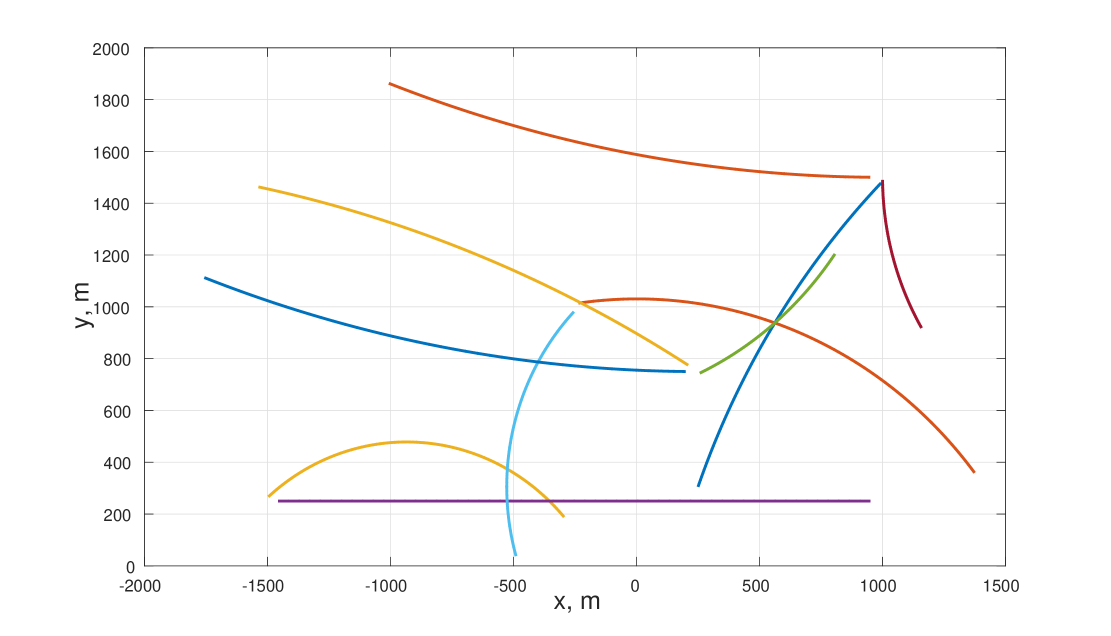
Figure 2: Cartesian coordinates for true target positions.

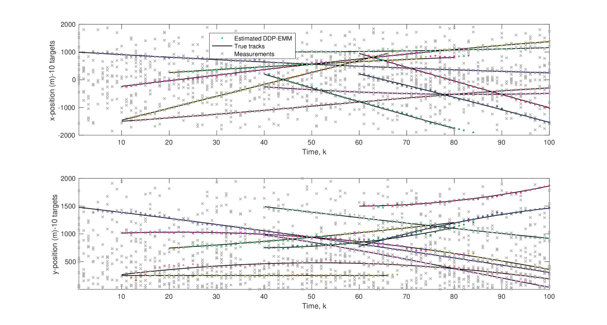
Figure 3: Actual and estimated (a) $x_{k}$ and (b) $y_{k}$ coordinates using DDP-EMM (all colors)

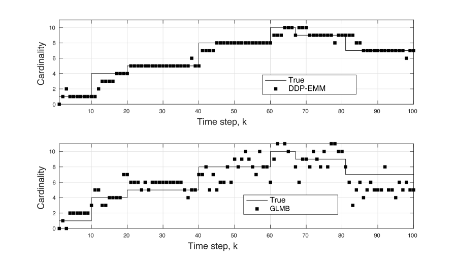
Figure 4: Estimated cardinality using DDP-EMM (top) and GLMB.

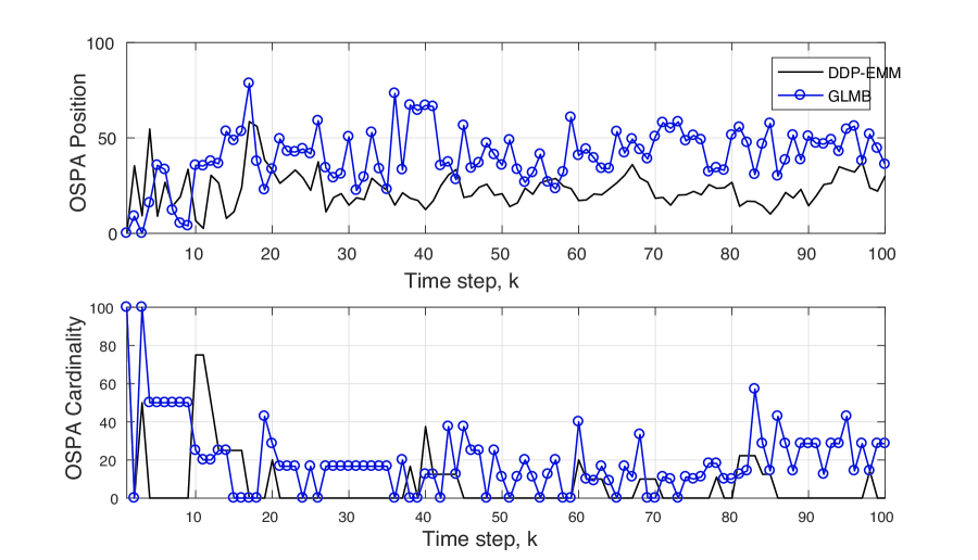
Figure 5: OSPA position and cardinality: DDP-EMM, GLMB.

Close Proximity

We consider a more complex scenario, where the targets are moving in close proximity to each other. A maximum of 5 targets enter the scene at different time steps but follow the same trajectory. As a result, they are expected to have the same position but at different time steps. The 5 targets enter the scene at corresponding time steps $k$ = $0$, $k$ = $5$, $k$ = $20$, $k$ = $30$, and $k$ = $40$; they leave the scene at corresponding time steps $k$ = $70$, $k$ = $100$, $k$ = $100$, $k$ = $45$, and $k$ = $80$. For this example, the NIW distribution used $\nu$ = $100$ and concentration parameter prior $\Gamma(\alpha;1,0.3)$. The estimated target position using DDP-EEM is shown in Fig. 6. The comparison between the DDP-EEM and GLMB for the estimated cardinality and OSPA metric are shown in Fig. 7 and 8, respectively. As demonstrated, the DDP-EMM performs much higher than the GLMB for closely-spaced targets.

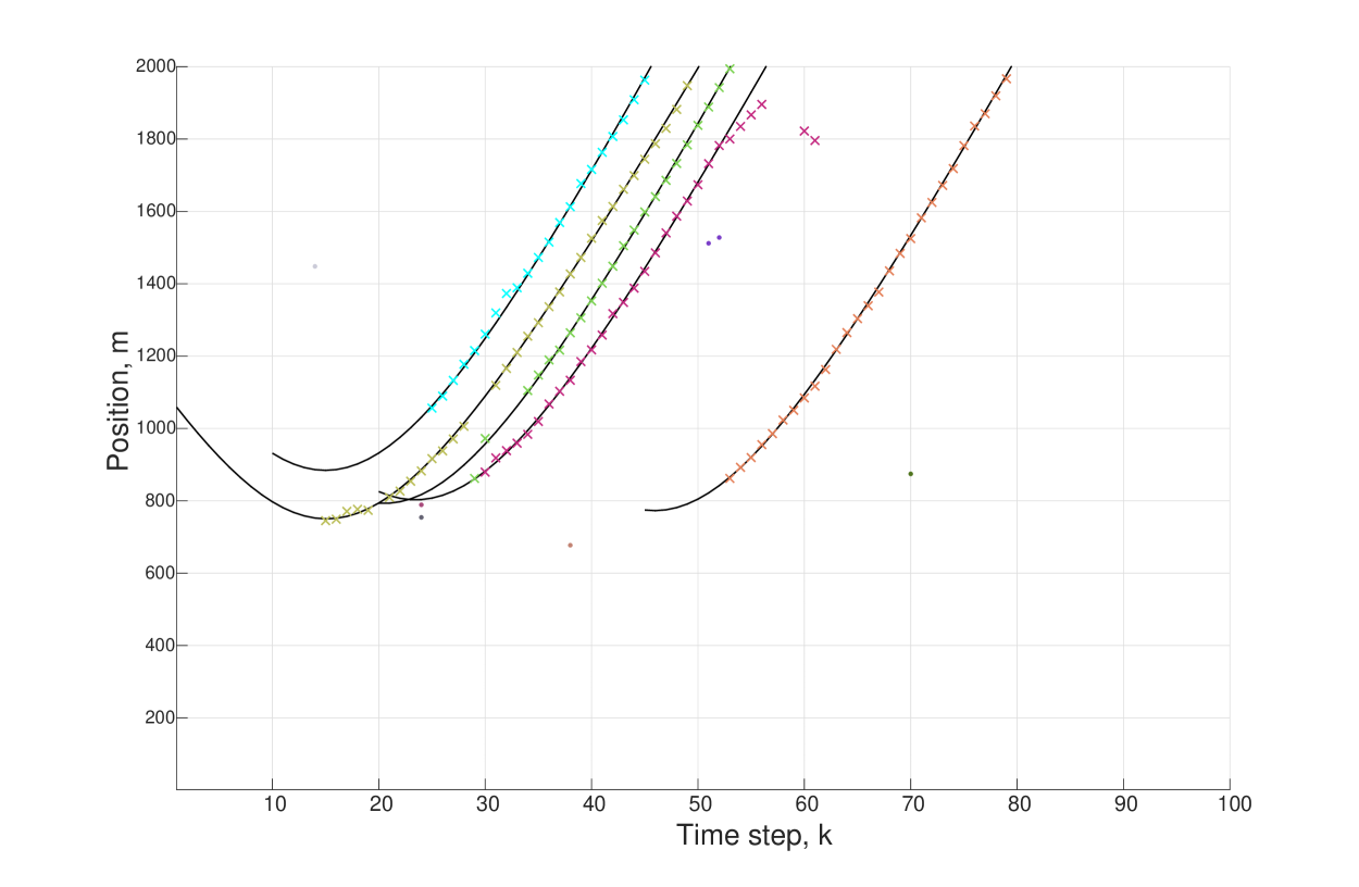
Figure 6: Estimated position using DDP-EM.

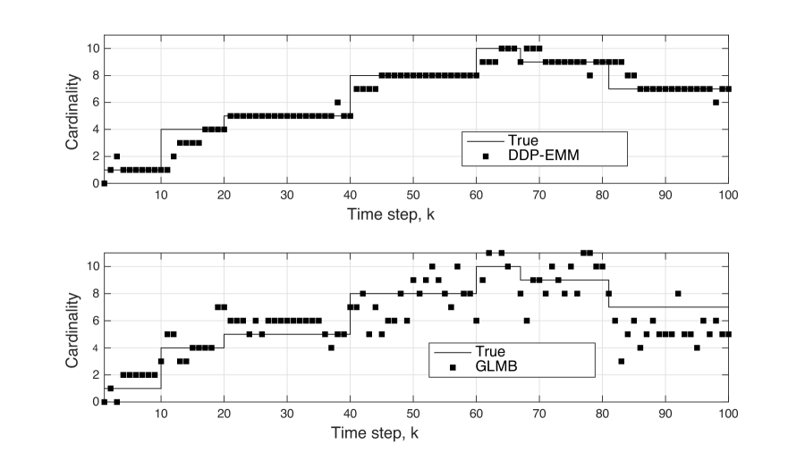
Figure 7: Estimated cardinality: DDP-EMM (top), GLMB.

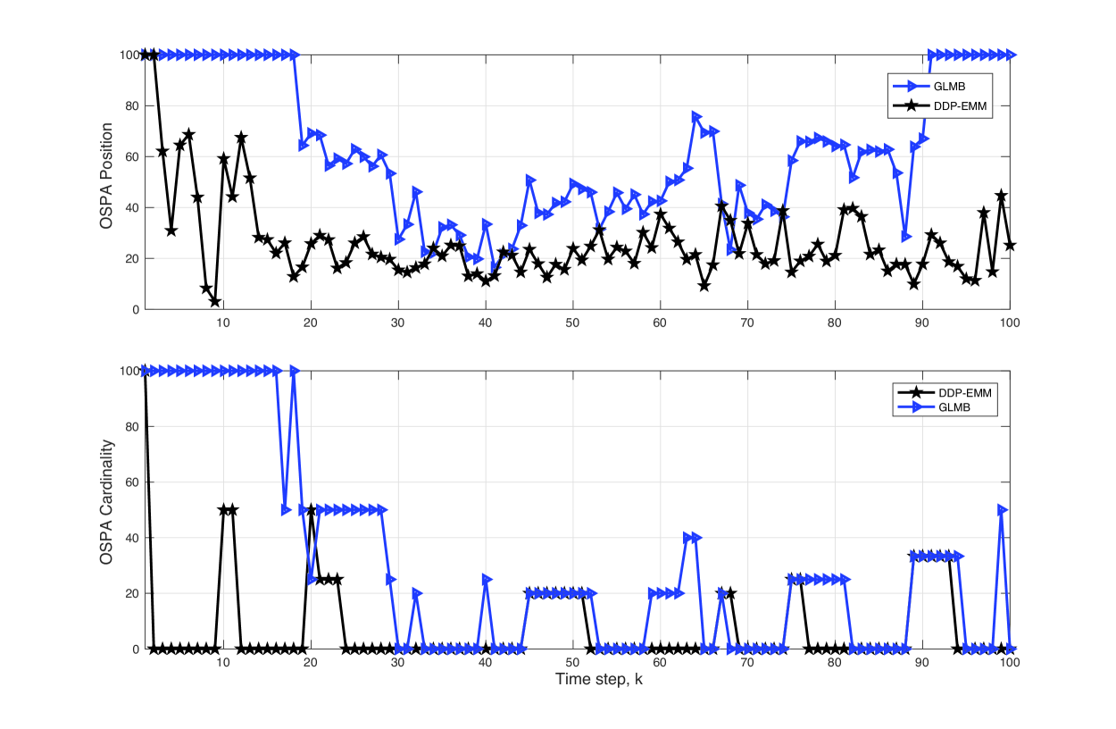
Figure 8: OSPA position and cardinality: DDP-EMM, GLMB.

Varying SNR

In this example, we assume that there are 11 targets with $\omega_{k}$ = $0$ and that only range measurements are available. We demonstrate the performance of the DDP-EMM approach for SNR values -3, -5 and -10 dB. For the simulations, $\mu_{0}$ = $0$ and $\nu$ = $100$ were used for the NIW distribution and the concentration prior was $\Gamma(\alpha;1,0.2)$. The cardinality performance for decreasing SNR is demonstrated in Fig. 9. As expected, the performance of the DDP-EMM decreases as the SNR decreases; however, the correct cardinality of the states was obtained most of times. Fig. 10 depicts the decrease in DDP-EMM OSPA performance as the SNR decreases.

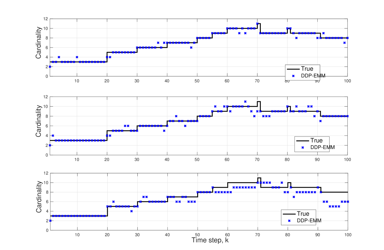
Figure 9: Cardinality estimation using DDP-EMM for -3 dB (top), -5 dB (middle), and -10 dB SNR (bottom).

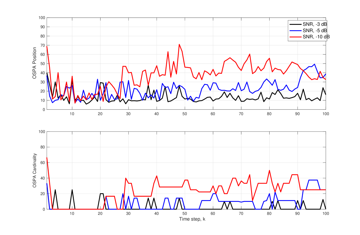
Figure 10: OSPA position (top) and cardinality (bottom) using DDP-EMM for -3 dB, -5 dB and -10 dB SNR.

DPY-STP and GLMB Comparison

The higher performance of the DPY-STP is demonstrated and compared to the GLMB using a maximum of 5 targets. This is shown in Fig. 11 and Fig. 12 with the estimated cardinality and the OSPA range and cardinality, respectively, for the two methods.

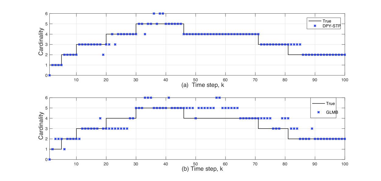
Figure 11: Cardinality estimation: (a) DPY-STP (b) GLMB

.

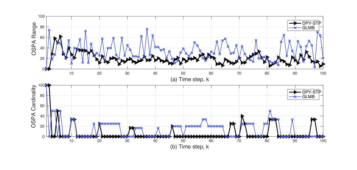
Figure 12: OSPA range & cardinality: DPY-STP, GLMB.

DPY-STP and DDP-EMM Comparison

As discussed in Section 5, the DPY is better matched to the tracking a TV number of objects than the DDP. This is demonstrated by comparing the DPY-STP and DDP-EMM methods using a maximum number of 10 targets. The simulations used $\mu_{0}$ = $0$ and $\nu$ = $100$ for the NIW distribution; parameters $\alpha$ and $d$ were selected using $\Gamma(\alpha;1,0.1)$. The estimated position using the two methods is shown in Fig. 13. The increased performance of the DPY-STP is shown using the OSPA comparison for position and cardinality in Fig. 14.

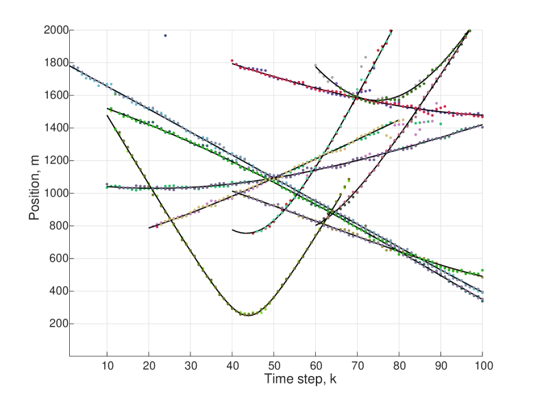
(a)

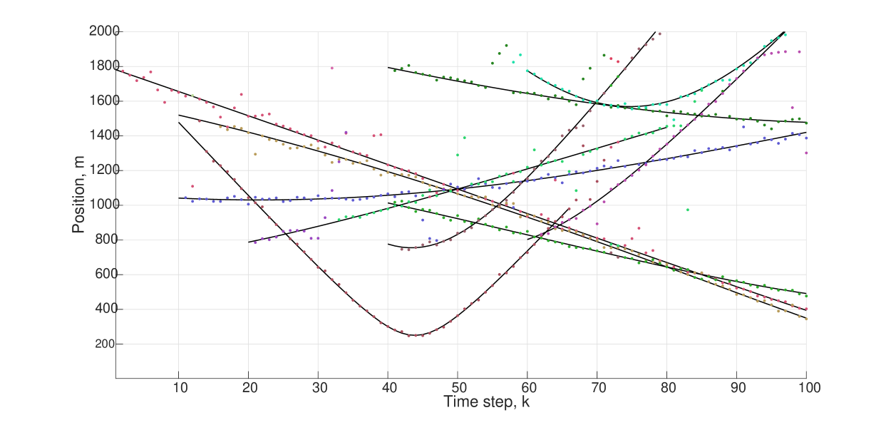
(b)

Figure 13: Position estimation: (a) DPY-STP (b) DDP-EMM.

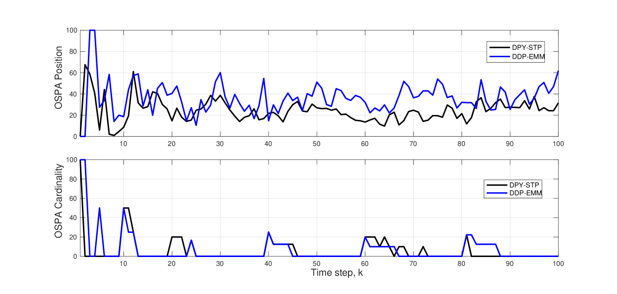
Figure 14: OSPA position & cardinality: DPY-STP, DDP-EMM.

7 Conclusion

We presented novel families of Bayesian nonparametric processes to capture the computational and inferential needs when tracking a TV number of objects. The proposed models offer improvements in tracking performance, time efficiency, and implementation cost. They exploit the dependent Dirichlet and dependent Pitman-Yor processes to model object priors to efficiently track object labels, cardinality and trajectories. Furthermore, MCMC implementation of the proposed tracking algorithms successfully verifies the simplicity and accuracy of proposed methods.

Acknowledgments

The authors would like to thank the anonymous referees, an Associate Editor and the Editor for their constructive comments that improved the quality of this paper.This work was supported in part by Grant AFOSR FA9550-17-1-0100

Appendix A.

In this appendix we prove the equation 14: Section 4.2:

Proof. Proof of 14 follows the standard Bayesian nonparametric methods. We know that the base measure in DP($\alpha$, H) is the mean of the Dirichlet prior. The following lemma generalizes this fact.

Lemma 1.

(Ferguson 1973, Ferguson (1973)) If $G\sim\text{DP}(\alpha,H)$ and $f$ is any measurable function, then

$$\mathbb{E}\Big{[}\int f(\theta)dG(\theta)\Big{]}=\int f(\theta)dH(\theta)$$

Suppose that $A$ and $B$ are measurable sets.

$$P(\theta_{\ell,k}\in A,\mathbf{z}_{\ell,k}\in B|\theta_{-\ell,k},\mathbf{z}_{-\ell,k})= \mathbb{E}\big{[}\mathbbm{1}_{\theta_{\ell,k}}(A)\mathbbm{1}_{\mathbf{z}_{\ell,k}}(B)|\theta_{-\ell,k},\mathbf{z}_{-\ell,k}\big{]}$$ (21)

$$= \mathbb{E}\Big{[}\mathbb{E}\big{[}\mathbbm{1}_{\theta_{\ell,k}}(A)\mathbbm{1}_{\mathbf{z}_{\ell,k}}(B)|G,\theta_{-\ell,k},\mathbf{z}_{-\ell,k}\big{]}|\theta_{-\ell,k},\mathbf{z}_{-\ell,k}\Big{]}$$ (22)

$$= \mathbb{E}\Big{[}\int\mathbbm{1}_{\theta_{\ell,k}}(A)\mathbbm{1}_{\mathbf{z}_{\ell,k}}(B)p(\mathbf{z}_{\ell,k}|\theta_{\ell,k},\mathbf{x}_{\ell,k})d\mathbf{z}_{\ell,k}dG({\theta_{\ell,k}}|{\theta_{-\ell,k}})\Big{]}$$ (23)

where 21 follows the definition of expected value, 22 is due to the law of iterated expectations, and $G(\theta)$ in 23 is the posterior dependent Dirichlet process given in 13. Using lemma 1

$$\mathbb{E}\Big{[}\int\mathbbm{1}_{\theta_{\ell,k}}(A)\mathbbm{1}_{\mathbf{z}_{\ell,k}}(B)p(\mathbf{z}_{\ell,k}|\theta_{\ell,k},\mathbf{x}_{\ell,k})d\mathbf{z}_{\ell,k}dG({\theta_{\ell,k}}|{\theta_{-\ell,k}})\Big{]}=$$ (24)

$$\int\mathbbm{1}_{\theta_{\ell,k}}(A)\mathbbm{1}_{\mathbf{z}_{\ell,k}}(B)p(\mathbf{z}_{\ell,k}|\theta_{\ell,k},\mathbf{x}_{\ell,k})d\mathbf{z}_{\ell,k}$$ (25)

$$d\Big{(}\sum\limits_{\Theta_{k}-\{\theta_{\ell,k}\}}\Pi_{1}\delta_{\theta}(\theta_{\ell,k})+\sum\limits_{\begin{subarray}{c}\theta\in\Theta^{\star}_{k|k-1}\setminus\Theta\\ \theta\neq\theta_{\ell,k}\end{subarray}}\Pi_{2}\nu({\bf{\theta}^{\star}_{\ell,k-1}},{\bf{\theta_{\ell,k}}})\delta_{\theta}({\bf{\theta_{\ell,k}}})+\Pi_{3}H(\theta_{\ell,k})\Big{)}.$$

Using the Bayes rule we have:

$$P(\theta_{\ell,k}\in A|\theta_{-\ell,k},\mathcal{Z}_{k})=\frac{\int_{B}P(\theta_{\ell,k}\in A,\mathbf{z}_{\ell,k}|\theta_{-\ell,k},\mathbf{z}_{-\ell,k})d\mathbf{z}_{\ell,k}}{\int_{\Omega}P(\theta_{\ell,k}\in A,\mathbf{z}_{\ell,k}|\theta_{-\ell,k},\mathbf{z}_{-\ell,k})d\mathbf{z}_{\ell,k}}$$ (26)

and this concludes the claim in 14.

References

- Ahmed and Xing (2008) Amr Ahmed and Eric Xing. Dynamic non-parametric mixture models and the recurrent Chinese restaurant process: With applications to evolutionary clustering. In SIAM International Conference on Data Mining, pages 219–230, 2008.
- Aldous (1985) David J Aldous. Exchangeability and related topics. In École d’Été de Probabilités de Saint-Flour XIII—1983, pages 1–198. Springer, 1985.
- Antoniak (1974) Charles E Antoniak. Mixtures of Dirichlet processes with applications to Bayesian nonparametric problems. Ann. Stat., pages 1152–1174, 1974.
- Aoki et al. (2016) E. H. Aoki, P. K. Mandal, L. Svensson, Y. Boers, and A. Bagchi. Labeling uncertainty in multitarget tracking. IEEE Transactions Aerospace Electronic Systems, 52:1006–1020, 2016.
- Bar-Shalom (1990) Yaakov Bar-Shalom. Multitarget-Multisensor Tracking: Advanced Applications. Artech House, 1990.
- Blei and Frazier (2011) David M Blei and Peter I Frazier. Distance dependent Chinese restaurant processes. J. Machine Learning Res., 12:2461–2488, 2011.
- Campbell et al. (2013) Trevor Campbell, Miao Liu, Brian Kulis, J. P. How, and Lawrence Carin. Dynamic clustering via asymptotics of the dependent Dirichlet process mixture. In Advances in Neural Information Proc. Systems, pages 449–457, 2013.
- Caron et al. (2007) François Caron, Manuel Davy, and Arnaud Doucet. Generalized Pólya urn for time-varying Dirichlet process mixtures. In Conference on Uncertainty in Artificial Intelligence, pages 33–40, 2007.
- Caron et al. (2017) François Caron, Willie Neiswanger, Frank Wood, Arnaud Doucet, and Manuel Davy. Generalized Pólya urn for time-varying Pitman-Yor processes. Journal of Machine Learning Research, 18(27):1–32, 2017.
- Choi1and and Ramamoorthi (2008) T. Choi1and and R. V. Ramamoorthi. Remarks on consistency of posterior distributions. IMS Collections, 3:170–186, 2008.
- Escobar (1994) Michael D Escobar. Estimating normal means with a Dirichlet process prior. J. American Statistical Association, 89:268–277, 1994.
- Escobar and West (1995) Michael D Escobar and Mike West. Bayesian density estimation and inference using mixtures. J. American Statistical Ass., 90:577–588, 1995.
- Ferguson (1973) Thomas S Ferguson. A Bayesian analysis of some nonparametric problems. The Annals of Statistics, pages 209–230, 1973.
- MacEachern (1999) S. N. MacEachern. Dependent nonparametric processes. In Proceedings of the Bayesian Statistical Science Section, 1999.
- MacEachern (2000) S. N. MacEachern. Dependent Dirichlet processes. Technical report, Department of Statistics, Ohio State University, 2000.
- MacEarchern (1998) S. N. MacEarchern. Computational methods for mixture of Dirichlet process models. In D. Dey et al., editors, Practical Nonparametric and Semiparametric Bayesian Statistics, volume 133. Springer, 1998.
- Mahler (2007) R. P. S. Mahler. Statistical Multisource-Multitarget Information Fusion. Artech House, 2007.
- Moraffah (2019a) Bahman Moraffah. Inference for multiple object tracking: A Bayesian nonparametric approach. arXiv preprint arXiv:1909.06984 cs.LG, 2019a.
- Moraffah (2019b) Bahman Moraffah. Bayesian Nonparametric Modeling and Inference for Multiple Object Tracking. PhD thesis, Arizona State University, 2019b.
- Moraffah and Papandreou-Suppappola (2018) Bahman Moraffah and Antonia Papandreou-Suppappola. Dependent dirichlet process modeling and identity learning for multiple object tracking. In 52nd Asilomar Conference on Signals, Systems, and Computers, pages 1762–1766. IEEE, 2018.
- Moraffah and Papandreou-Suppappola (2019) Bahman Moraffah and Antonia Papandreou-Suppappola. Random infinite tree and dependent Poisson diffusion process for nonparametric Bayesian modeling in multiple object tracking. In IEEE International Conference on Acoustics, Speech and Signal Processing (ICASSP), pages 5217–5221. IEEE, 2019.
- Moraffah et al. (2019a) Bahman Moraffah, Cesar Brito, Bindya Venkatesh, and Antonia Papandreou-Suppappola. Tracking multiple objects with multimodal dependent measurements: Bayesian nonparametric modeling. In 2019 53rd Asilomar Conference on Signals, Systems, and Computers, pages 1847–1851. IEEE, 2019a.
- Moraffah et al. (2019b) Bahman Moraffah, Cesar Brito, Bindya Venkatesh, and Antonia Papandreou-Suppappola. Use of hierarchical dirichlet processes to integrate dependent observations from multiple disparate sensors for tracking. In 2019 22th International Conference on Information Fusion (FUSION), pages 1–7. IEEE, 2019b.
- Moraffah et al. (2019c) Bahman Moraffah, Antonia Papandreou-Suppappola, and Muralidhar Rangaswamy. Nonparametric bayesian methods and the dependent pitman-yor process for modeling evolution in multiple object tracking. In 2019 22th International Conference on Information Fusion (FUSION), pages 1–6. IEEE, 2019c.
- Neiswanger et al. (2014) Willie Neiswanger, Frank Wood, and Eric Xing. The dependent Dirichlet process mixture of objects for detection-free tracking and object modeling. In Int. Conf. Artificial Intelligence and Statistics, pages 660–668, 2014.
- Pitman (2002) Jim Pitman. Poisson-Dirichlet and GEM invariant distributions for split-and-merge transformations of an interval partition. Combinatorics, Probability and Computing, 11(5):501–514, 2002.
- Pitman and Yor (1997) Jim Pitman and Marc Yor. The two-parameter Poisson-Dirichlet distribution derived from a stable subordinator. Annals of Prob., pages 855–900, 1997.
- Reuter et al. (2014) S. Reuter, B.-T. Vo, B.-N. Vo, and K. Dietmayer. The labeled multi-Bernoulli filter. IEEE Transactions on Signal Processing, 62:3246–3260, 2014.
- Sethuraman (1994) Jayaram Sethuraman. A constructive definition of Dirichlet priors. Statistica Sinica, pages 639–650, 1994.
- Teh (2006) Yee Whye Teh. A hierarchical Bayesian language model based on Pitman-Yor processes. In Int. Conf. Comput. Linguistics, pages 985–992, 2006.
- Teh (2011) Yee Whye Teh. Dirichlet process. In Encyclopedia of Machine Learning, pages 280–287. Springer, 2011.
- Topkaya et al. (2013) Ibrahim Saygin Topkaya, Hakan Erdogan, and Fatih Porikli. Detecting and tracking unknown number of objects with Dirichlet process mixture models and Markov random fields. In International Symposium on Visual Computing, pages 178–188, 2013.
- Vo et al. (2015) B.-N. Vo, M. Mallick, Y. Bar-Shalom, S. Coraluppi, R. Osborne III, R. Mahler, and B.-T Vo. Multitarget tracking. Wiely Enc. of Electrical Eng., 2015.
- Vo et al. (2014) Ba-Ngu Vo, Ba-Tuong Vo, and Dinh Phung. Labeled random finite sets and the Bayes multi-target tracking filter. IEEE Transactions on Signal Processing, 62:6554–6567, 2014.
- Vo et al. (2017) Ba-Ngu Vo, Ba-Tuong Vo, and Hung Gia Hoang. An efficient implementation of the generalized labeled multi-Bernoulli filter. IEEE Transactions on Signal Processing, 65(8):1975–1987, 2017.
- Wang et al. (2017) X. Wang, T. Li, S. Sun, and J. M. Corchado. A survey of recent advances in particle filters and remaining challenges for multitarget tracking. Sensors, 17:12, 2017.