Learning to Classify Intents and Slot Labels Given a Handful of Examples

Abstract

Intent classification (IC) and slot filling (SF) are core components in most goal-oriented dialogue systems. Current IC/SF models perform poorly when the number of training examples per class is small. We propose a new few-shot learning task, few-shot IC/SF, to study and improve the performance of IC and SF models on classes not seen at training time in ultra low resource scenarios. We establish a few-shot IC/SF benchmark by defining few-shot splits for three public IC/SF datasets, ATIS, TOP, and Snips. We show that two popular few-shot learning algorithms, model agnostic meta learning (MAML) and prototypical networks, outperform a fine-tuning baseline on this benchmark. Prototypical networks achieves significant gains in IC performance on the ATIS and TOP datasets, while both prototypical networks and MAML outperform the baseline with respect to SF on all three datasets. In addition, we demonstrate that joint training as well as the use of pre-trained language models, ELMo and BERT in our case, are complementary to these few-shot learning methods and yield further gains.

1 Introduction

In the context of goal-oriented dialogue systems, intent classification (IC) is the process of classifying a user’s utterance into an intent, such as BookFlight or AddToPlaylist, referring to the user’s goal. While slot filling (SF) is the process of identifying and classifying certain tokens in the utterance into their corresponding labels, in a manner akin to named entity recognition (NER). However, in contrast to NER, typical slots are particular to the domain of the dialogue, such as music or travel. As a reference point, we list intent and slot label annotations for an example utterance from the Snips dataset with the AddToPlaylist IC in Figure 1.

Token	Slot Label
Please	O
add	O
some	O
Pete	AddToPlaylist:artist
Townshend	AddToPlaylist:artist
to	O
my	AddToPlaylist:playlist_owner
playlist	O
Fiesta	AddToPlaylist:playlist
Hits	AddToPlaylist:playlist
con	AddToPlaylist:playlist
Lali	AddToPlaylist:playlist

Figure 1: Tokens and corresponding slot labels for an utterance from the AddToPlaylist intent class in the Snips dataset prefixed by intent class name.

As of late, most state-of-the-art IC/SF models are based on feed-forward, convolutional, or recurrent neural networks Hakkani-Tür et al. (2016); Goo et al. (2018); Gupta et al. (2019). These neural models offer substantial gains in performance, but they often require a large number of labeled examples (on the order of hundreds) per intent class and slot-label to achieve these gains. The relative scarcity of large-scale datasets annotated with intents and slots prohibits the use of neural IC/SF models in many promising domains, such as medical consultation, where it is difficult to obtain large quantities of annotated dialogues.

Accordingly, we propose the task of few-shot IC/SF, catering to domain adaption in low resource scenarios, where there are only a handful of annotated examples available per intent and slot in the target domain. To the best of our knowledge, this work is the first to apply the few-shot learning framework to a joint sentence classification and sequence labeling task. In the NLP literature, few-shot learning often refers to a low resource, cross lingual setting where there is limited data available in the target language. We emphasize that our definition of few-shot IC/SF is distinct in that we limit the amount of data available per target class rather than target language.

Few-shot IC/SF builds on a large body of existing few-shot classification work. Drawing inspiration from computer vision, we experiment with two prominent few shot image classification approaches, prototypical networks and model agnostic meta learning (MAML). Both these methods seek to decrease over-fitting and improve generalization on small datasets, albeit via different mechanisms. Prototypical networks learns class specific representations, called prototypes, and performs inference by assigning the class label associated with the prototype closest to an input embedding. Whereas MAML modifies the learning objective to optimize for pre-training representations that transfer well when fine-tuned on a small number of labeled examples.

For benchmarking purposes, we establish few-shot splits for three publicly available IC/SF datasets: ATIS Hemphill et al. (1990), Snips Coucke et al. (2018), and TOP Gupta et al. (2018). Empirically, prototypical networks yields substantial improvements on this benchmark over the popular “fine-tuning” approach Goyal et al. (2018); Schuster et al. (2018), where representations are pre-trained on a large, “source” dataset and then fine-tuned on a smaller, “target” dataset. Despite performing worse on intent classification, MAML also achieves gains over “fine-tuning” on the slot filling task. Orthogonally, we experiment with the use of two pre-trained language models, BERT and ELMo, as well as joint training on multiple datasets. These experiments show that the use of pre-trained, contextual representations is complementary to both methods. While prototypical networks is uniquely able to leverage joint training to consistently boost slot filling performance.

In summary, our primary contributions are four-fold:

1. Formulating IC/SF as a few-shot learning task;

2. Establishing few-shot splits for the ATIS, Snips, and TOP datasets;

3. Showing that MAML and prototypical networks can outperform the popular “fine-tuning” domain adaptation framework;

4. Evaluating the complementary of contextual embeddings and joint training with MAML and prototypical networks.

2 Related Work

2.1 Few-shot Learning

Early adoption of few-shot learning in the field of computer vision has yielded promising results. Neural approaches to few-shot learning in computer vision fall mainly into three categories: optimization-, metric-, or memory-based. Optimization-based methods typically learn an initialization or fine-tuning procedure for a neural network. For instance, MAML Finn et al. (2017) directly optimizes for representations that generalize well to unseen classes given a few labeled examples. Using an LSTM based meta-learner, Ravi and Larochelle (2016) learn both the initialization and the fine-tuning procedure. In contrast, metric-based approaches learn an embedding space or distance metric under which examples belonging to the same class have high similarity. Prototypical networks Snell et al. (2017), siamese neural networks Koch (2015), and matching networks Vinyals et al. (2016) all belong to this category. Alternatively, memory based approaches apply memory modules or recurrent networks with memory, such as a LSTM, to few-shot learning. These approaches include differentiable extensions to k-nearest-neighbors Kaiser et al. (2017) and applications of the Neural Turing Machines Graves et al. (2014); Santoro et al. (2016).

2.2 Few-shot Learning for Text Classification

To date, applications of few-shot learning to natural language processing focus primarily on text classification tasks. Yu et al. (2018) identify “clusters” of source classification tasks that transfer well to a given target task, and meta learn a linear combination of similarity metrics across “clusters”. The source tasks with the highest likelihood of transfer are used to pre-train a convolutional network that is subsequently fine-tuned on the target task. Han et al. (2018) propose FewRel, a few-shot relation classification dataset, and use this data to benchmark the performance of few-shot models, such as prototypical networks and SNAIL Mishra et al. (2017). ATAML Jiang et al. (2018), one of the few optimization based approaches to few-shot sentence classification, extends MAML to learn task-specific as well as task agnostic representations using feed-forward attention mechanisms. Dou et al. (2019) show that further pre-training of contextual representations using optimization-based methods benefits downstream performance.

2.3 Few-shot Learning for Sequence Labeling

In one of the first works on few-shot sequence labeling, Fritzler et al. (2019) apply prototypical networks to few-shot named entity recognition by training a separate prototypical network for each named entity type. This design choice makes their extension of prototypical networks more restrictive than ours, which trains a single model to classify all sequence tags. Hou et al. (2019) apply a CRF based approach that learns emission scores using pre-trained, contextualized embeddings to few-shot SF (on Snips) and few-shot NER.

3 Task Formulation

3.1 Few-shot Classification

The goal of few-shot classification is to adapt a classifier $f_{\phi}$ to a set of new classes $L$ not seen at training time, given a few labeled examples per class $l\in L$. In this setting, train and test splits are defined by disjoint class label sets $L_{train}$ and $L_{test}$, respectively. The classes in $L_{train}$ are made available for pre-training and those in $L_{test}$ are held out for low resource adaptation at test time. Few-shot evaluation is done episodically, i.e. over a number of mini adaptation datasets, called episodes. Each episode consists of a support set $S$ and a query set $Q$. The support set contains $k_{l}$ labeled examples $S_{l}=\{(x_{l}^{i},y_{l})|i{\in}(1{\ldots}k_{l})\}$ per held out class $l\in L$; we define $S=\bigcup_{l\in L}S_{l}$. Similarly, the query set contains $k_{q}$ labeled instances $Q_{l}=\{(x_{l}^{j},y_{l})|j{\in}(1{\ldots}k_{q})\}$ for each class $l\in L$ s.t. $Q_{l}\cap S_{l}=\{\}$; we define $Q=\bigcup_{l\in L}Q_{l}$. The support set provides a few labeled examples of new classes not seen at training time that $f_{\phi}$ must adapt to i.e. learn to classify, whereas the query set is used for evaluation. Few-shot classification requires episodic evaluation; however, most few-shot learning methods train as well as evaluate on episodes. Consistent with prior work, we train both MAML and prototypical networks methods on episodes, as opposed to mini-batches.

3.2 Few-shot IC/SF

Few-shot IC/SF extends the prior definition of few-shot classification to include both IC and SF tasks. As Geng et al. (2019) showed, it is straightforward to formulate IC as a few-shot classification task. Simply let the class labels $y_{l}$ in section 3.1 correspond to IC labels and partition the set of ICs into the train and test splits, $L_{train}$ and $L_{test}$. Building on this few-shot IC formulation, we re-define the support and query sets to include the slots $t_{l}$, in addition the intent $y_{l}$, assigned to each example $x_{l}$. Thus, the set of support and query instances for class $l\in L$ become $S_{l}=\{(x_{l}^{i},t_{l}^{i},y_{l})|i{\in}(1{\ldots}k_{l})\}$ and $Q_{l}=\{(x_{l}^{j},t_{l}^{j},y_{l})|j{\in}(1{\ldots}k_{q})\}$, respectively. To construct an episode, we sample a total of $k_{l}+k_{q}$ labeled examples per IC $l\in L$ to form the support and query sets. Since many slot-label sequences may belong to the same IC, it is possible to sample an episode such that a slot-label in the query set does not appear in the support set or vice versa. Therefore, to ensure fair evaluation, we map any slot-label in the query set that does not occur in the support set or vice versa to “Other”, which is ignored by our SF evaluation metric.

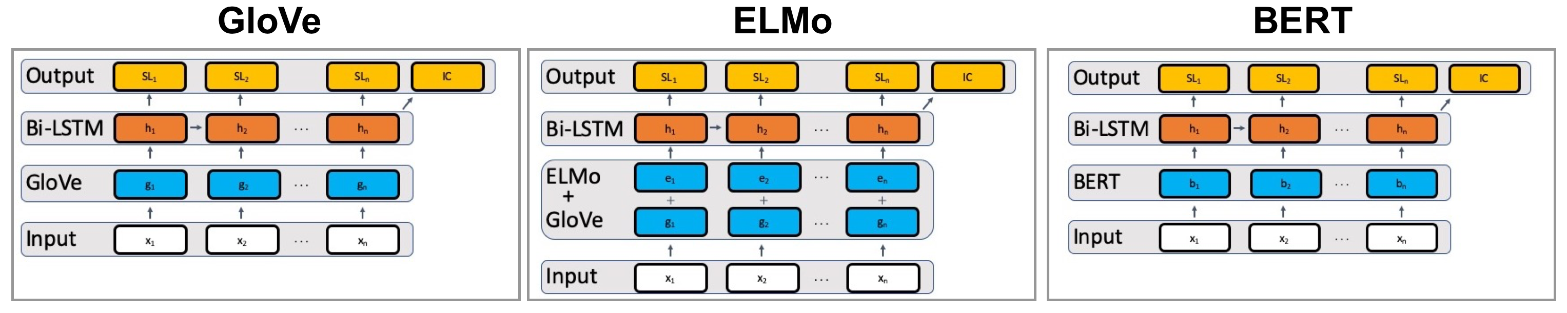
Figure 2: Three model architectures, each consisting of an embedding layer, comprised of either GloVe word embeddings (GloVe), GloVe word embeddings concatenated with ELMo embeddings (ELMo), or BERT embeddings (BERT), that feed into a bi-directional LSTM, which is followed by fully connected intent and slot output layers.

4 Approach

4.1 Prototypical Networks for Joint Intent Classification and Slot Filling

The original formulation of prototypical networks Snell et al. (2017) is not directly applicable to sequence labeling. Accordingly, we extend prototypical networks to perform joint sentence classification and sequence labeling. Our extension computes “prototypes” $c_{l}$ and $c_{a}$ for each intent class $l$ and slot-label $a$, respectively. Each prototype $c\in\mathbb{R^{D}}$ is the mean vector of the embeddings belonging to a given intent class or slot-label class. These embeddings are output by a sequence encoder $f_{\phi}(x):\rightarrow\mathbb{R}^{D}$, which takes a variable length utterance of $m$ tokens $x^{i}=(x^{i}_{1},x^{i}_{2},\dots,x^{i}_{m})$ as input, and outputs the final hidden state $h\in\mathbb{R}^{D}$ of the encoder. For ease of notation, let $S_{l}=\{(x_{l}^{i},t_{l}^{i},y_{l})\}$ be the support set instances with intent class $y_{l}$. And let $S_{a}=\{(x^{i}_{[1:j]},t^{i}_{[1:j]},y^{i})|t^{i}_{j}=a\}$ be the support set sub-sequences with slot-label $a$ for the token $x^{i}_{j}$ in $x^{i}$. Using this notation, we calculate slot-label and intent class prototypes as follows:

$$c_{l} =\frac{1}{|S_{l}|}\sum_{(x^{i},t^{i},y_{l})\in S_{l}}f_{\phi}(x^{i})$$ (1)

$$c_{a} =\frac{1}{|S_{a}|}\sum_{(x^{i}_{[1:j]},\>t^{i}_{[1:j]},\>y^{i})}f_{\phi}(x^{i}_{[1:j]})$$ (2)

Given an example $(x^{*},t^{*},y^{*})\in Q$, we compute the conditional probability $p(y=l\mid x^{*},S)$ that the utterance $x^{*}$ has intent class $l$ as the normalized Euclidean distance between $f_{\phi}(x^{*})$ and the prototype $c_{l}$,

$$p(y=l\mid x^{*},S)=\frac{\exp(-\left\lVert f_{\phi}(x^{*})-c_{l}\right\rVert_{2}^{2})}{\sum_{l^{\prime}}\exp(-\left\lVert f_{\phi}(x^{*})-c_{l^{\prime}}\right\rVert_{2}^{2})}$$

Similarly, we compute the conditional probability $p(t^{*}_{j}=a\mid x^{*},S)$ that the j-th token $x^{*}_{j}$ in the utterance $x^{*}$ has slot-label $t^{*}_{j}=a$ as the normalized Euclidean distance between $f_{\phi}(x^{*}_{[1:j]})$ and the prototype $c_{a}$,

$$p(t^{*}_{j}=a\mid x^{*},S)=\frac{\exp(-\left\lVert f_{\phi}(x^{*}_{[1:j]})-c_{a}\right\rVert_{2}^{2})}{\sum_{a^{\prime}}\exp(-\left\lVert f_{\phi}(x^{*}_{[1:j]})-c_{a^{\prime}}\right\rVert_{2}^{2})}$$

We define the joint IC and SF prototypical loss function $\mathcal{L}_{proto}$ as the sum of the IC and SF negative log-likelihoods averaged over the query set instances given the support set:

$$\mathcal{L}_{proto}=\frac{1}{|Q|}\sum_{(x^{*},t^{*},y^{*})\in Q}\mathcal{L}_{protoIC}+\mathcal{L}_{protoSF}$$

$$\mathcal{L}_{protoIC}=-\log p(y=y^{*}\mid x^{*},S)$$

$$\mathcal{L}_{protoSF}=-\sum_{t^{*}_{j}\in t^{*}}\log p(t^{*}_{j}=a\mid x^{*},S)$$

4.2 Model Agnostic Meta Learning (MAML)

MAML optimizes the parameters $\phi$ of the encoder $f_{\phi}$ such that when $\phi$ is fine-tuned on the support set $S$ for $d$ steps, $\phi^{\prime}\leftarrow\mbox{Finetune}(\phi,d\>|S)$, the fine-tuned model $f_{\phi^{\prime}}$ generalizes well to new class instances in the query set $Q$. This is achieved by updating $\phi$ to minimize the loss of the fine-tuned model $\mathcal{L}(f_{\phi^{\prime}},Q)$ on the query set $Q$. The update to $\phi$ takes the form $\phi\leftarrow\phi-\nabla_{\phi}\mathcal{L}(f_{\phi^{\prime}},Q)$, where $\mathcal{L}$ is the sum of IC and SF softmax cross entropy loss functions. Concretely, given a support and query set $(S,Q)$, MAML performs the following two step optimization procedure:

$$1.\>\>\phi^{\prime}\leftarrow\mbox{Finetune}(\phi,d\>|S)$$

$$2.\>\>\phi\leftarrow\phi-\nabla_{\phi}\mathcal{L}(f_{\phi^{\prime}},Q)$$

Although, the initial formulation of MAML, which we outline here, utilizes stochastic gradient descent (SGD) to update the initial parameters $\phi$, in practice, an alternate gradient based update rule can be used in place of SGD. Empirically, we find it beneficial to use Adam in place of SGD.

A drawback to MAML is that computing the “meta-gradient” $\nabla_{\phi}\mathcal{L}(f_{\phi^{\prime}},Q)$ requires calculating a second derivative, since the gradient must backpropagate through the sequence of updates made by $\mbox{Finetune}(\phi,d\>|S)$. Fortunately, in the same work where Finn et al. (2017) introduce MAML, they propose a first order approximation of MAML, foMAML, which ignores these second derivative terms and performs nearly as well as the original method. We utilize foMAML in our experiments to avoid memory issues associated with MAML.

Split	ATIS				Snips				TOP
	#Utt	#IC	#SL	#SV	#Utt	#IC	#SL	#SV	#Utt	#IC	#SL	#SV
Train	4,373	5	116	461	8,230	4	33	8,549	20,345	7	38	5,574
Dev	662	7	122	260	-	-	-	-	4,333	5	33	2,228
Test	829	7	128	258	6,254	3	20	7,567	4,426	6	39	1,341
Total	5,864	19	366	583	14,484	7	53	13,599	29,104	18	110	6821

Table 1: Statistics on utterance (Utt), intent (IC), slot label (SL), and slot value (SV) counts for ATIS, TOP, and Snips few-shot train, development, and test splits as well as the full dataset, provided under the heading total.

5 Few-shot IC/SF Benchmark

As there is no existing benchmark for few-shot IC/SF, we propose few-shot splits for the Air Travel Information System (ATIS, Hemphill et al. (1990)), Snips Coucke et al. (2018), and Task Oriented Parsing (TOP, Gupta et al. (2018)) datasets. A few-shot IC/SF benchmark is beneficial for two reasons. Firstly, the benchmark evaluates generalization across multiple domains. Secondly, researchers can combine these datasets in the future to experiment with larger settings of $n$-way during training and evaluation.

5.1 Datasets

ATIS is a well-known dataset for dialog system research, which comprises conversations from the airline domain. Snips, on the other hand, is a public benchmark dataset developed by the Snips corporation to evaluate the quality of IC and SF services. The Snips dataset comprises multiple domains including music, media, and weather. TOP, which pertains to navigation and event search, is unique in that 35% of the utterances contain multiple, nested intent labels. These hierarchical intents require the use of specialized models. Therefore, we utilize only the remaining, non-hierarchical 65% of utterances in TOP. To put the size and diversity of these datasets in context, we provide utterance, intent, slot-label, and slot value counts for each dataset in table 1.

5.2 Few-shot Splits

We target train, development, and test split sizes of 70%, 15%, and 15%, respectively. However, the ICs in these datasets are highly imbalanced, which prevents us from hitting these targets exactly. Thereby, we manually select the ICs to include in each split. For the Snips dataset, we choose not to form a development split because there are only 7 ICs in the Snips dataset, and we require a minimum of 3 ICs per split. During preprocessing we modify slot label names by adding the associated IC as a prefix to each slot. This preprocessing step ensures that the slot labels are no longer pure named entities, but specific semantic roles in the context of particular intents. In table 1, we provide statistics on the few-shot splits for each dataset.

6 Experiments

6.1 Episode Construction

For train and test episodes, we sample both the the number of classes in each episode, the “way” $n$, and the number of examples to include for each sampled class $l$, the class “shot” $k_{l}$, using the procedure put forward in Triantafillou et al. (2019). By sampling the shot and way, we allow for unbalanced support sets and a variable number of classes per episode. These allowances are compatible with the large degree of class imbalances present in our benchmark, which would make it difficult to apply a fixed shot and way for all intents.

To construct an episode given a few-shot class split $L_{split}$, we first sample the way $n$ uniformly from the range $[3,|L_{split}|]$. We then sample $n$ intent classes uniformly at random from $L_{split}$ to form $L$. Next, we sample the query shot $k_{q}$ for the episodes as follows:

$$k_{q}=\min(10,(\min_{l\in L}\>[0.5\>*|X_{l}|]))$$

where $X_{l}$ is the set of examples with class label $l$. Given the query shot $k_{q}$, we compute the target support set size for the episode as:

$$|S|\>=\min(K_{\max},\sum_{l\in L}\lceil\beta\min(20,|X_{l}|-\>q)\rceil)$$

where $\beta$ is sampled uniformly from the range $(0,1]$ and $K_{\max}$ is the maximum episode size. Lastly, we sample the support shot $k_{l}$ for each class as:

$$k_{l}=\min(\lfloor R_{l}*(|S|-|L|)\rfloor+1,|X_{l}|-\>q)$$

where $R_{l}$ is a noisy estimate of the normalized proportion of the dataset made up by class $l$, which we compute as follows:

$$R_{l}=\frac{\exp(\alpha_{l})*|X_{l}|}{\sum_{l^{\prime}\in L}\exp(\alpha_{l^{\prime}})*|X_{l^{\prime}}|)}$$

The noise in our estimate of the proportion $R_{l}$ is introduced by sampling the value of $\alpha_{l}$ uniformly from the interval $[\log(0.5),\log(2))$.

6.2 Episode Sizes

We present IC/SF results for two settings of maximum episode size, $K_{\max}=20$ and $K_{\max}=100$, in tables 2/4 and 3/5, respectively. When the maximum episode size $K_{\max}=20$, the average support set shot $k_{l}$ is 3.58 for ATIS, 3.78 for TOP, and 5.22 for Snips. In contrast, setting the maximum episode size to $K_{\max}=100$ increases the average support set shot $k_{l}$ to 9.15 for ATIS, 9.81 for TOP, and 10.83 for Snips.

6.3 Training Settings

In our experiments, we consider two training settings. One in which we train on episodes, or batches in the case of our baseline, from a single dataset. And another, joint training approach that randomly selects the dataset from which to sample a given episode/batch. After sampling an episode, we remove its contents from a buffer of available examples. If there are no longer enough examples in the buffer to create an episode, we refresh the buffer to contain all examples.

6.4 Network Architecture

The network architectures we explore, depicted in Figure 2, consist of an embedding layer, a sequence encoder, and two output layers for slots and intents, respectively. Each architecture uses a different pre-trained embedding layer type, which are either non-contextual or contextual. We experiment with one non-contextual embedding, GloVe word vectors Pennington et al. (2014), as well as two contextual embeddings, GloVe concatenated with ELMo embeddings Peters et al. (2018), and BERT embeddings Devlin et al. (2018). The sequence encoder is a bi-directional LSTM Hochreiter and Schmidhuber (1997) with a 512-dimensional hidden state. Output layers are fully connected and take concatenated forward and backward LSTM hidden states as input. Pre-trained embeddings are kept frozen for training and adaptation. Attempts to fine-tune BERT led to inferior results. We refer to each architecture by its embedding type, namely GloVe, ELMo, or BERT.

6.5 Baseline

We compare the performance of our approach against a Fine-tune baseline, which implements the domain adaptation framework commonly applied to low resource IC/SF Goyal et al. (2018). We pre-train the Fine-tune baseline, either jointly or individually, on the classes in our training split(s). Then at evaluation time, we freeze the pre-trained encoder and “fine-tune” new output layers for the slots and intents included in the support set. This fine-tuned model is then used to predict the intent and slots for each held out example in the query set.

6.6 Hyper-parameters

We train all models using the Adam optimizer Kingma and Ba (2014). We use the default learning rate of 0.001 for the baseline and prototypical networks. For foMAML we set the outer learning rate to 0.0029 and finetune for $d=8$ steps with an inner learning rate of 0.01. We pre-train the Fine-tune baseline with a batch size of 512. At test time, we fine-tune the baseline for 10 steps on the support set. We train the models without contextual embeddings (GloVe alone) for 50 epochs and those with contextual ELMo or BERT embeddings for 30 epochs because they exhibit faster convergence.

6.7 Evaluation Metrics

To assess the performance of our models, we report the average IC accuracy and slot F1 score over 100 episodes sampled from the test split of an individual dataset. We use the AllenNLP Gardner et al. (2017) CategoricalAccuracy implementation to compute IC Accuracy. And to compute slot F1 score, we use the seqeval library’s span based F1 score implementation. The span based F1 score is a relatively harsh metric in the sense that a slot label prediction is only considered correct if the slot label and span exactly match the ground truth annotation.

Embed.	Algorithm	IC Accuracy
		Snips	Snips (joint)	ATIS	ATIS (joint)	TOP	TOP (joint)
GloVe	Fine-tune	69.52 +/- 2.88	70.25 +/- 1.85	49.50 +/- 0.65	58.26 +/- 1.12	37.58 +/- 0.54	40.93 +/- 2.77
GloVe	foMAML	61.08 +/- 1.50	59.67 +/- 2.12	54.66 +/- 1.82	45.20 +/- 1.47	33.75 +/- 1.30	31.48 +/- 0.50
GloVe	Proto	68.19 +/- 1.76	68.77 +/- 1.60	65.46 +/- 0.81	63.91 +/- 1.27	43.20 +/- 0.85	38.65 +/- 1.35
ELMo	Fine-tune	85.53 +/- 0.35	87.64 +/- 0.73	49.25 +/- 0.74	58.69 +/- 1.56	45.49 +/- 0.61	47.63 +/- 2.75
ELMo	foMAML	78.90 +/- 0.77	78.86 +/- 1.31	53.90 +/- 0.96	52.47 +/- 2.86	38.67 +/- 1.02	36.49 +/- 0.99
ELMo	Proto	83.54 +/- 0.40	85.75 +/- 1.57	65.95 +/- 2.29	65.19 +/- 1.29	50.57 +/- 2.81	50.64 +/- 2.72
BERT	Fine-tune	76.04 +/- 8.84	77.53 +/- 5.69	43.76 +/- 4.61	50.73 +/- 3.86	39.21 +/- 3.09	40.86 +/- 3.75
BERT	foMAML	67.36 +/- 1.03	68.37 +/- 0.48	50.27 +/- 0.69	48.80 +/- 2.82	38.50 +/- 0.43	36.20 +/- 1.21
BERT	Proto	81.39 +/- 1.85	81.44 +/- 2.91	58.84 +/- 1.33	58.82 +/- 1.55	52.76 +/- 2.26	52.64 +/- 2.58

Table 2: $K_{\max}=20$ average IC accuracy on 100 test episodes from the ATIS, Snips, or TOP datasets in the form mean $\pm$ standard deviation, computed over 3 random seeds, comparing GloVe, ELMo, and BERT model variants for both individual and joint training, where we train on all training sets and test on a specific test set.

Embed.	Algorithm	IC Accuracy
		Snips	Snips (joint)	ATIS	ATIS (joint)	TOP	TOP (joint)
GloVe	Fine-tune	72.24 +/- 2.58	73.00 +/- 1.84	49.91 +/- 1.90	56.07 +/- 2.94	39.66 +/- 1.34	41.10 +/- 0.65
GloVe	foMAML	66.75 +/- 1.28	67.34 +/- 2.62	54.92 +/- 0.87	58.46 +/- 1.91	33.62 +/- 1.53	35.68 +/- 0.62
GloVe	Proto	70.45 +/- 0.49	72.66 +/- 1.96	70.25 +/- 0.39	69.58 +/- 0.41	48.84 +/- 1.59	46.85 +/- 0.86
ELMo	Fine-tune	87.69 +/- 1.05	88.90 +/- 0.18	49.42 +/- 0.79	56.99 +/- 2.12	47.44 +/- 1.61	48.87 +/- 0.54
ELMo	foMAML	80.80 +/- 0.47	81.62 +/- 1.07	59.10 +/- 2.52	56.16 +/- 1.34	41.80 +/- 1.49	36.24 +/- 0.79
ELMo	Proto	86.76 +/- 1.62	87.74 +/- 1.08	70.10 +/- 1.26	71.89 +/- 1.45	58.60 +/- 1.91	56.87 +/- 0.39
BERT	Fine-tune	76.66 +/- 8.68	79.53 +/- 4.25	44.08 +/- 6.05	49.71 +/- 3.84	40.05 +/- 2.35	40.46 +/- 1.74
BERT	foMAML	70.43 +/- 1.56	72.79 +/- 1.11	51.36 +/- 3.74	50.25 +/- 0.88	36.15 +/- 2.17	35.24 +/- 0.35
BERT	Proto	83.51 +/- 0.88	86.29 +/- 1.09	66.89 +/- 2.31	65.70 +/- 2.31	61.30 +/- 0.32	62.51 +/- 1.79

Table 3: $K_{\max}=100$ average IC accuracy on 100 test episodes from the ATIS, Snips, or TOP datasets in the form mean $\pm$ standard deviation, computed over 3 random seeds, comparing GloVe, ELMo, and BERT model variants for both individual and joint training, where we train on all training sets and test on a specific test set.

Embed.	Algorithm	Slot F1 Measure
		Snips	Snips (joint)	ATIS	ATIS (joint)	TOP	TOP (joint)
GloVe	Fine-tune	6.72 +/- 1.24	6.68 +/- 0.40	2.57 +/- 1.21	13.22 +/- 1.07	0.90 +/- 0.51	0.76 +/- 0.21
GloVe	foMAML	14.07 +/- 1.01	12.91 +/- 0.43	18.44 +/- 0.91	16.91 +/- 0.32	5.34 +/- 0.43	9.22 +/- 1.03
GloVe	Proto	29.63 +/- 0.75	27.75 +/- 2.52	31.19 +/- 1.15	38.45 +/- 0.97	10.65 +/- 0.83	18.55 +/- 0.35
ELMo	Fine-tune	22.02 +/- 1.13	16.00 +/- 2.07	7.47 +/- 2.60	7.19 +/- 1.71	1.26 +/- 0.46	1.17 +/- 0.32
ELMo	foMAML	33.81 +/- 0.33	32.82 +/- 0.84	27.58 +/- 1.25	24.45 +/- 1.20	22.35 +/- 1.23	15.53 +/- 0.64
ELMo	Proto	59.88 +/- 0.53	59.73 +/- 1.72	33.97 +/- 0.38	40.90 +/- 2.21	20.12 +/- 0.25	28.97 +/- 0.82
BERT	Fine-tune	12.47 +/- 0.31	8.75 +/- 0.28	9.24 +/- 1.67	15.93 +/- 3.10	3.15 +/- 0.28	1.08 +/- 0.30
BERT	foMAML	12.72 +/- 0.12	13.28 +/- 0.53	18.91 +/- 1.01	16.05 +/- 0.32	5.93 +/- 0.43	8.23 +/- 0.81
BERT	Proto	42.09 +/- 1.11	43.77 +/- 0.54	37.61 +/- 0.82	39.27 +/- 1.84	20.81 +/- 0.40	28.24 +/- 0.53

Table 4: $K_{\max}=20$ average Slot F1 score on 100 test episodes from the ATIS, Snips, or TOP datasets in the form mean $\pm$ standard deviation, computed over 3 random seeds, comparing GloVe, ELMo, and BERT model variants for both individual and joint training, where we train on all training sets and test on a specific test set.

Embed.	Algorithm	Slot F1 Measure
		Snips	Snips (joint)	ATIS	ATIS (joint)	TOP	TOP (joint)
GloVe	Fine-tune	7.06 +/- 1.87	7.76 +/- 0.91	2.72 +/- 1.65	17.20 +/- 3.03	1.26 +/- 0.44	0.67 +/- 0.33
GloVe	foMAML	16.77 +/- 0.67	16.53 +/- 0.32	17.80 +/- 0.42	23.33 +/- 2.89	4.11 +/- 0.81	9.89 +/- 1.13
GloVe	Proto	31.57 +/- 1.28	31.17 +/- 1.31	31.32 +/- 2.79	41.07 +/- 1.14	9.99 +/- 1.08	18.93 +/- 0.77
ELMo	Fine-tune	22.37 +/- 0.91	17.09 +/- 2.57	8.93 +/- 2.86	11.09 +/- 2.00	2.04 +/- 0.41	1.03 +/- 0.24
ELMo	foMAML	36.10 +/- 1.49	37.33 +/- 0.24	26.91 +/- 2.64	26.37 +/- 0.15	18.32 +/- 0.52	16.55 +/- 0.79
ELMo	Proto	62.71 +/- 0.40	62.14 +/- 0.75	35.20 +/- 2.46	41.28 +/- 2.73	18.44 +/- 2.41	28.33 +/- 1.33
BERT	Fine-tune	14.71 +/- 0.43	10.50 +/- 0.90	11.53 +/- 1.46	20.41 +/- 1.85	4.98 +/- 0.66	1.48 +/- 0.85
BERT	foMAML	14.99 +/- 1.29	15.83 +/- 0.94	17.68 +/- 2.42	17.11 +/- 1.31	3.37 +/- 0.36	10.58 +/- 0.45
BERT	Proto	46.50 +/- 0.75	48.77 +/- 0.71	40.63 +/- 3.37	43.10 +/- 1.76	20.58 +/- 2.27	28.92 +/- 1.09

Table 5: $K_{\max}=100$ average Slot F1 score on 100 test episodes from the ATIS, Snips, or TOP datasets in the form mean $\pm$ standard deviation, computed over 3 random seeds, comparing GloVe, ELMo, and BERT model variants for both individual and joint training, where we train on all training sets and test on a specific test set.

7 Results

7.1 Few-shot Learning Algorithms

Prototypical networks

Considering both IC and SF tasks, prototypical networks is the best performing algorithm. The most successful variant of prototypical networks, Proto ELMo + joint training, obtains absolute improvements over the Fine-tune ELMo + joint training baseline of up to 6% IC accuracy and 43 slot F1 points for $K_{max}=20$, and 14% IC accuracy and 45 slot F1 points for $K_{max}=100$. The one case in which Proto ELMo + joint training does worse than the baseline is on Snips IC, but these losses are all under 2%.

foMAML

The results for foMAML are more mixed in terms of IC and SF performance relative to the baseline. The best foMAML variant, foMAML ELMo, underperforms Fine-tune ELMo on Snips and TOP IC by up to 6%. Yet foMAML improves IC accuracy by 4% ($K_{max}=20$) to 9% ($K_{max}=100$) on ATIS. foMAML ELMo consistently outperforms Fine-tune ELMo on SF for all datasets, generating gains of 11$\sim$21 F1 points for $K_{max}=20$ and 13$\sim$17 F1 points for $K_{max}=100$. Notably, BERT and foMAML in combination do not work well. Specifically, the SF performance of foMAML BERT is comparable to, or worse than, foMAML GloVe on all datasets for both $K_{max}=20$ and $K_{max}=100$.

7.2 Model Variants

Non-contextual Pretrained Embeddings

The GloVe model architecture, which uses GloVe alone, does not perform as well as ELMo or BERT. On average over experimental settings, the GloVe variant of the winning algorithm has 10% lower IC Accuracy and 16 point lower slot F1 score than the winning algorithm paired with the best model. Note that an experimental setting here refers to a combination of dataset, value of $K_{max}$, and use of individual or joint training. Somewhat surprisingly, GloVe performs nearly as well as ELMo and even better than BERT on ATIS IC. We speculate that ATIS IC does not benefit as much from the use of ELMo or BERT because ATIS carrier phrases are less diverse, as evidenced by the smaller number of unique carrier phrases in the ATIS test set (527) compared to Snips (3,718) and TOP (4,153).

Contextual Pretrained Embeddings

A priori, it is reasonable to suspect that the performance gain obtained by our few-shot learning algorithms could be dwarfed by the benefit of using a large, pre-trained model like ELMo or BERT. However, our experimental results suggest that the use of pre-trained language models is complementary to our approach, in most cases. For example, ELMo increases the slot F1 score of foMAML from 14.07 to 33.81 and boosts the slot F1 of prototypical networks from 31.57 to 62.71 on the Snips dataset for $K_{max}=100$. Similarly, when $K_{max}=20$, BERT improves foMAML and prototypical networks TOP IC accuracy from 33.75% to 38.50% and from 43.20% to 52.76%, respectively. In aggregate, we find ELMo outperforms BERT. We quantify this via the average absolute improvement ELMo obtains over BERT when both models use the winning algorithm for a given dataset and training setting. On average, ELMo improves IC accuracy over BERT by 2% for $K_{max}=20$ and 1% for $K_{max}=100$. With respect to slot F1 score, ELMo produces an average gain over BERT of 5 F1 points for $K_{max}=20$ and 3 F1 points for $K_{max}=100$. This is consistent with previous findings in Peters et al. (2019) that ELMo can outperform BERT on certain tasks when the models are kept frozen and not fine-tuned.

7.3 Joint Training

Few-shot learning algorithms are in essence learning to learn new classes. Therefore, these algorithms should be better suited to leverage a diverse training dataset to improve generalization. We test this hypothesis by jointly training each approach on all three datasets. Our results demonstrate that joint training has little effect on IC Accuracy; however, it improves the SF performance of prototypical networks, particularly on ATIS and TOP. Joint training increases Prototypical networks average slot F1 score, computed over datasets and model variants, by 4.41 points from 31.77 to 36.18 for $K_{max}=20$ and by 5.20 points from 32.99 to 38.19 when $K_{max}=100$. In comparison, Fine-tune obtains much smaller average absolute improvements, 0.55 F1 points and 1.29 F1 points for $K_{max}=20$ and $K_{max}=100$, respectively.

8 Conclusion

This work shows the benefit of applying few-shot learning techniques to few-shot IC/SF. Specifically, our extension of prototypical networks for joint IC and SF consistently outperforms a fine-tuning based method with respect to both IC Accuracy and slot F1 score. The use of this prototypical approach in combination with pre-trained language models, such as ELMo, generates additional performance improvements, especially on the SF task. While our contribution is a step toward the creation of more sample efficient IC/SF models, there is still substantial work to be done in pursuit of this goal, especially in the creation of larger few-shot IC/SF benchmarks. We encourage the creation of a large scale IC and SF dataset to test how these methods scale with larger episode sizes and view this direction as a high leverage way to further this line of research.

References

- Coucke et al. (2018) Alice Coucke, Alaa Saade, Adrien Ball, Théodore Bluche, Alexandre Caulier, David Leroy, Clément Doumouro, Thibault Gisselbrecht, Francesco Caltagirone, Thibaut Lavril, Maël Primet, and Joseph Dureau. 2018. Snips voice platform: an embedded spoken language understanding system for private-by-design voice interfaces. CoRR, abs/1805.10190.
- Devlin et al. (2018) Jacob Devlin, Ming-Wei Chang, Kenton Lee, and Kristina Toutanova. 2018. Bert: Pre-training of deep bidirectional transformers for language understanding. arXiv preprint arXiv:1810.04805.
- Dou et al. (2019) Zi-Yi Dou, Keyi Yu, and Antonios Anastasopoulos. 2019. Investigating meta-learning algorithms for low-resource natural language understanding tasks. arXiv preprint arXiv:1908.10423.
- Finn et al. (2017) Chelsea Finn, Pieter Abbeel, and Sergey Levine. 2017. Model-agnostic meta-learning for fast adaptation of deep networks. In Proceedings of the 34th International Conference on Machine Learning-Volume 70, pages 1126–1135. JMLR. org.
- Fritzler et al. (2019) Alexander Fritzler, Varvara Logacheva, and Maksim Kretov. 2019. Few-shot classification in named entity recognition task. In Proceedings of the 34th ACM/SIGAPP Symposium on Applied Computing, pages 993–1000. ACM.
- Gardner et al. (2017) Matt Gardner, Joel Grus, Mark Neumann, Oyvind Tafjord, Pradeep Dasigi, Nelson F. Liu, Matthew Peters, Michael Schmitz, and Luke S. Zettlemoyer. 2017. Allennlp: A deep semantic natural language processing platform.
- Geng et al. (2019) Ruiying Geng, Binhua Li, Yongbin Li, Yuxiao Ye, Ping Jian, and Jian Sun. 2019. Few-shot text classification with induction network. arXiv preprint arXiv:1902.10482.
- Goo et al. (2018) Chih-Wen Goo, Guang Gao, Yun-Kai Hsu, Chih-Li Huo, Tsung-Chieh Chen, Keng-Wei Hsu, and Yun-Nung Chen. 2018. Slot-gated modeling for joint slot filling and intent prediction. In Proceedings of the 2018 Conference of the North American Chapter of the Association for Computational Linguistics: Human Language Technologies, Volume 2 (Short Papers), pages 753–757.
- Goyal et al. (2018) Anuj Goyal, Angeliki Metallinou, and Spyros Matsoukas. 2018. Fast and scalable expansion of natural language understanding functionality for intelligent agents. arXiv preprint arXiv:1805.01542.
- Graves et al. (2014) Alex Graves, Greg Wayne, and Ivo Danihelka. 2014. Neural turing machines. arXiv preprint arXiv:1410.5401.
- Gupta et al. (2019) Arshit Gupta, John Hewitt, and Katrin Kirchhoff. 2019. Simple, fast, accurate intent classification and slot labeling. arXiv preprint arXiv:1903.08268.
- Gupta et al. (2018) Sonal Gupta, Rushin Shah, Mrinal Mohit, Anuj Kumar, and Mike Lewis. 2018. Semantic parsing for task oriented dialog using hierarchical representations. In Proceedings of the 2018 Conference on Empirical Methods in Natural Language Processing, pages 2787–2792, Brussels, Belgium. Association for Computational Linguistics.
- Hakkani-Tür et al. (2016) Dilek Hakkani-Tür, Gökhan Tür, Asli Celikyilmaz, Yun-Nung Chen, Jianfeng Gao, Li Deng, and Ye-Yi Wang. 2016. Multi-domain joint semantic frame parsing using bi-directional rnn-lstm. In Interspeech, pages 715–719.
- Han et al. (2018) Xu Han, Hao Zhu, Pengfei Yu, Ziyun Wang, Yuan Yao, Zhiyuan Liu, and Maosong Sun. 2018. Fewrel: A large-scale supervised few-shot relation classification dataset with state-of-the-art evaluation. In Proceedings of the 2018 Conference on Empirical Methods in Natural Language Processing, pages 4803–4809.
- Hemphill et al. (1990) Charles T Hemphill, John J Godfrey, and George R Doddington. 1990. The atis spoken language systems pilot corpus. In Speech and Natural Language: Proceedings of a Workshop Held at Hidden Valley, Pennsylvania, June 24-27, 1990.
- Hochreiter and Schmidhuber (1997) Sepp Hochreiter and Jürgen Schmidhuber. 1997. Long short-term memory. Neural computation, 9(8):1735–1780.
- Hou et al. (2019) Yutai Hou, Zhihan Zhou, Yijia Liu, Ning Wang, Wanxiang Che, Han Liu, and Ting Liu. 2019. Few-shot sequence labeling with label dependency transfer. arXiv preprint arXiv:1906.08711.
- Jiang et al. (2018) Xiang Jiang, Mohammad Havaei, Gabriel Chartrand, Hassan Chouaib, Thomas Vincent, Andrew Jesson, Nicolas Chapados, and Stan Matwin. 2018. Attentive task-agnostic meta-learning for few-shot text classification.
- Kaiser et al. (2017) Łukasz Kaiser, Ofir Nachum, Aurko Roy, and Samy Bengio. 2017. Learning to remember rare events. arXiv preprint arXiv:1703.03129.
- Kingma and Ba (2014) Diederik P Kingma and Jimmy Ba. 2014. Adam: A method for stochastic optimization. arXiv preprint arXiv:1412.6980.
- Koch (2015) Gregory Koch. 2015. Siamese neural networks for one-shot image recognition.
- Mishra et al. (2017) Nikhil Mishra, Mostafa Rohaninejad, Xi Chen, and Pieter Abbeel. 2017. A simple neural attentive meta-learner. arXiv preprint arXiv:1707.03141.
- Pennington et al. (2014) Jeffrey Pennington, Richard Socher, and Christopher Manning. 2014. Glove: Global vectors for word representation. In Proceedings of the 2014 conference on empirical methods in natural language processing (EMNLP), pages 1532–1543.
- Peters et al. (2018) Matthew E. Peters, Mark Neumann, Mohit Iyyer, Matt Gardner, Christopher Clark, Kenton Lee, and Luke Zettlemoyer. 2018. Deep contextualized word representations. In Proc. of NAACL.
- Peters et al. (2019) Matthew E. Peters, Sebastian Ruder, and Noah A. Smith. 2019. To tune or not to tune? adapting pretrained representations to diverse tasks. In Proceedings of the 4th Workshop on Representation Learning for NLP (RepL4NLP-2019), pages 7–14, Florence, Italy. Association for Computational Linguistics.
- Ravi and Larochelle (2016) Sachin Ravi and Hugo Larochelle. 2016. Optimization as a model for few-shot learning.
- Santoro et al. (2016) Adam Santoro, Sergey Bartunov, Matthew Botvinick, Daan Wierstra, and Timothy Lillicrap. 2016. Meta-learning with memory-augmented neural networks. In International conference on machine learning, pages 1842–1850.
- Schuster et al. (2018) Sebastian Schuster, Sonal Gupta, Rushin Shah, and Mike Lewis. 2018. Cross-lingual transfer learning for multilingual task oriented dialog. arXiv preprint arXiv:1810.13327.
- Snell et al. (2017) Jake Snell, Kevin Swersky, and Richard Zemel. 2017. Prototypical networks for few-shot learning. In Advances in Neural Information Processing Systems, pages 4077–4087.
- Triantafillou et al. (2019) Eleni Triantafillou, Tyler Zhu, Vincent Dumoulin, Pascal Lamblin, Kelvin Xu, Ross Goroshin, Carles Gelada, Kevin Swersky, Pierre-Antoine Manzagol, and Hugo Larochelle. 2019. Meta-dataset: A dataset of datasets for learning to learn from few examples. arXiv preprint arXiv:1903.03096.
- Vinyals et al. (2016) Oriol Vinyals, Charles Blundell, Timothy Lillicrap, Daan Wierstra, et al. 2016. Matching networks for one shot learning. In Advances in neural information processing systems, pages 3630–3638.
- Yu et al. (2018) Mo Yu, Xiaoxiao Guo, Jinfeng Yi, Shiyu Chang, Saloni Potdar, Yu Cheng, Gerald Tesauro, Haoyu Wang, and Bowen Zhou. 2018. Diverse few-shot text classification with multiple metrics. In Proceedings of the 2018 Conference of the North American Chapter of the Association for Computational Linguistics: Human Language Technologies, Volume 1 (Long Papers), pages 1206–1215.