Bosonization in 2+1 dimensions via Chern-Simons bosonic particle-vortex duality

Abstract

Dualities provide deep insight into physics by relating two seemingly distinct theories. Here we consider a duality between lattice fermions and bosons in (2+1) spacetime dimensions, relating free massive Dirac fermions to Abelian Chern-Simons Higgs (ACSH) bosons. To establish the duality we represent the exact partition function of the lattice fermions in terms of the writhe of fermionic worldlines. On the bosonic side the partition function is expressed in the writhe of the vortex loops of the particle-vortex dual of the ACSH Lagrangian. In the continuum and scaling limit we show these to be identical. This result can be understood from the closed fermionic worldlines being direct mappings of the ACSH vortex loops, with the writhe keeping track of particle statistics.

I Introduction

A duality transformation relates two theories that appear to be very different. Such a mapping is particularly useful if a seemingly hard question in one theory duality-transforms into a simple one in another theory. Duality transformations for example often invert the coupling constant in the dual theory, thereby transforming strongly interacting models into weakly interacting ones and vice versa Savit (1980); Kleinert (1989). In other cases, the transformation of the coupling constant is not a simple inversion, but rather a more complex function of the original one. Analyzing the properties of this function typically still allows to obtain results that would be difficult to achieve otherwise. A well known example is provided by the two-dimensional Ising model, whose dual model is again an Ising model. In this case the self-duality allows an exact determination of the critical temperature by just looking for the fixed point of the duality transformation, a result obtained before Onsager derived the exact solution of the model Kramers and Wannier (1941).

Of particular interest are dualities that implement a transmutation of particle statistics in addition to a mapping of coupling constants. In one-dimensional quantum systems (1+1 dimensions) such transmuting mappings between fermionic theories and bosonic ones are well-known and go under the general name of bosonization. Due to the fermionic sign structure of the wavefunction the situation is however much more complex in higher dimensions. In recent years there has been an intense activity surrounding bosonization dualities in 2+1 dimensions Seiberg et al. (2016); Karch and Tong (2016); Mross et al. (2017); Aharony et al. (2017); Benini (2018); Chen et al. (2018); Ferreiros and Fradkin (2018); Nastase and Núñez (2018); Wang et al. (2017); Dutta and Shankar (2008); Santos et al. (2020), but indeed it has turned out to be very difficult to obtain exact statements. For instance, while the free massive Dirac fermion in 1+1 dimensions can be exactly mapped into a sine-Gordon model with a particular value of the coupling constant Zinn-Justin (2002); Witten (1984); Stone (1994), a similar statement in 2+1 dimensions is argued to hold only at the infrared stable fixed point of the dual bosonic theory. The latter is given in this case by the following Abelian Chern-Simons Higgs (ACSH) Lagrangian,

$$\mathcal{L} = \frac{1}{4\pi}\epsilon_{\mu\nu\lambda}a^{\mu}\partial^{\nu}a^{\lambda}+|(\partial_{\mu}-ia_{\mu})\phi|^{2}$$ (1)

$$- m^{2}|\phi|^{2}-\frac{\lambda}{2}|\phi|^{4}.$$

A particularly simple classical soliton solution arises in the form of a so-called ”self-dual” CS vortices Jackiw and Weinberg (1990), where ”self-dual” here means the saturation of the Bogomolny bound Manton and Sutcliffe (2004) for the energy, achieved for a certain values of the coupling constants, which generally leads to first-order differential equations for the fields rather than second-order ones. The static vortex solution obtained in this way features a nonzero angular momentum, which is a direct consequence of the Chern-Simons (CS) term. It is interesting to note that a nonzero angular momentum for vortices is forbidden in the case of an ordinary Abelian Higgs model featuring a Maxwell term but sans CS term Julia and Zee (1975). But this no-go theorem does not hold for the theory (1) as due to the CS term the magnetic flux becomes the source of electric fields. A closely related result has been discussed recently in the context of an axion electrodynamics of vortices for a superconductor-topological insulator structure Nogueira et al. (2018). The remarkable fact is that for the case of a CS coupling as given in Eq. (1), the total angular momentum associated to the electromagnetic field and vortex is quantized in units of $\hbar/2$ which implies that the CS term transmutes the vortex into a fermion. Thus this soliton solution of the classical field equations already suggests a boson-fermion transmutation required by bosonization techniques.

Historically boson-fermion transmutation within a bosonization framework in 2+1 dimensions has been first discussed by Polyakov Polyakov (1988) for a model closely related to (1), namely, the CP^N-1 model with a CS term. Polyakov’s approach has been elaborated further in Refs. Grundberg et al. (1989); Shaji et al. (1990); Grundberg et al. (1990) and provides an early instance where the mapping of bosons to free massive Dirac fermions in 2+1 dimensions is discussed.

One of the main results of this paper is to establish a correspondence between free massive Dirac lattice fermions and the bosonic particle-vortex duality of Lagrangian (1) in the continuum limit using an exact representation of the partition function of Wilson fermions in terms of the writhe associated with the fermionic particle worldlines. Particle-vortex dualities for the Abelian Higgs model (sans CS term) in 2+1 dimensions are well established in several different, but closely related approaches Peskin (1978); Thomas and Stone (1978); Dasgupta and Halperin (1981); Kleinert (1982, 1989): it consists in mapping the worldline of a particle in a system with global $U(1)$ symmetry (for instance, the XY model) to vortex lines of the Abelian Higgs model. This particle-vortex duality does not involve a change of statistics, as both sides of the duality involve bosonic fields only. But it suggests a pathway to establish the bosonization duality in 2+1 dimensions: mapping the worldline of free massive fermions to the vortex loops of the Abelian Chern-Simons Higgs (ACSH) model (1). Interestingly, the lattice form of the ACSH Lagrangian (1) can be mapped by means of an exact duality to a Lagrangian of almost the same form Rey and Zee (1991), differing from the original Lagrangian by the presence of a Maxwell term.

The bosonization duality in 2+1 dimensions can be established exactly in the ultraviolet (UV) regime Chen et al. (2018) and is assumed to hold only approximately in the infrared regime (IR). This makes it important to establish a correspondence between the bosonic particle-vortex duality and the bosonization duality in a way that is as exact as possible. This is not an obvious task, since integrating out the bosonic matter fields in Eq. (1) leads to a self-linking of vortex loops, which is a less obvious occurrence in free massive Dirac fermions, as first realized by Polyakov Polyakov (1988).

The plan of the paper is as follows. In Section II we discuss the properties of the effective action of the bosonic theory, which prepares us for the identification of closed particle worldlines to vortex loops in later sections. In Section III the fermionic sector of the duality will be considered in the lattice using the Wilson fermion technique. Since the theory is Gaussian, the partition function can be obtained exactly in the thermodynamic limit. However, in 2+1 dimensions free massive Dirac fermions exhibit a nontrivial topology which can only be unveiled via a subtle path integral representation of the fermion determinant, $\det(\gamma^{\mu}\partial_{\mu}+m_{F})$ Polyakov (1988); Goldman and Fradkin (2018). In fact, despite the absence of interactions with a gauge field, the topologically nontrivial feature associated to the parity anomaly is already apparent from a straightforward exact calculation of the current correlation function. On the lattice we determine the fermion partition function by means of a hopping parameter expansion in a way similar to Ref. Stamatescu (1982). This allows an exact representation of the partition function as a summation over the weights of the all possible fermion worldlines, which are closed loops characterized by the writhe number. The way the writhe arises here is a consequence of the interplay between parity symmetry breaking (due to the mass) and the nontrivial topology of spinors in 2+1 dimensions. In Section IV we discuss the convergence of the hopping expansion and cast the partition function in a form more appropriate to relate to the bosonic dual partition function. The latter is discussed in Section V, where the duality transformation will be performed exactly on the lattice, where in the dual model the CS coupling is inverted. The bosonization duality implies that any side of the particle-vortex duality can in principle be mapped to the Lagrangian of a free massive Dirac fermion. This fact necessarily constraints the CS coupling to have the form given in Eq. (1). We emphasize here the important role of the writhe number that naturally emerges when analyzing vortex loops in CS theories Forte (1992). In Section V we show that the partition function of the dual ACSH theory is given as summation of the weight of the all possible vortex loop configurations, where we characterize the weight of the vortex loops in terms of the writhe of the loops. Finally, in Section VI the bosonization duality is established in the low energy vortex sector.

II Bosonic particle-vortex duality, and properties of the bosonic continuum actions

We begin by analyzing the (purely bosonic) particle-vortex duality of the ACSH Lagrangian. For a general CS coupling $\theta/\pi$, the duality takes the form,

$$\mathcal{L}_{b} = \frac{i\theta}{4\pi^{2}}\epsilon_{\mu\nu\lambda}a^{\mu}\partial^{\nu}a^{\lambda}+|(\partial_{\mu}-ia_{\mu})\phi|^{2}$$

$$+ m_{\text{B}}^{2}|\phi|^{2}+\frac{\lambda}{2}|\phi|^{4}$$

$$~{}~{}~{}~{}~{}~{}~{}~{}~{}~{}\Updownarrow{}$$

$$\tilde{\mathcal{L}}_{b} = \frac{1}{2e^{2}}(\epsilon_{\mu\nu\lambda}\partial^{\nu}b^{\lambda})^{2}+\frac{i\theta_{\text{D}}}{4\pi^{2}}\epsilon_{\mu\nu\lambda}b^{\mu}\partial^{\nu}b^{\lambda}$$ (2b)

$$+ |(\partial_{\mu}-ib_{\mu})\tilde{\phi}|^{2}+\tilde{m}_{\text{B}}^{2}|\tilde{\phi}|^{2}+\frac{\tilde{\lambda}}{2}|\tilde{\phi}|^{4}$$

where $\theta_{D}=-4\pi^{4}/\theta$. Unlike the free fermionic action

$$\mathcal{L}_{f} =\bar{\psi}(\gamma^{\mu}\partial_{\mu}+m_{\text{F}})\psi,$$ (3)

the bosonic fields in Eqs. (2) are interacting. A duality between Eqs. (2) and (3) can therefore only hold in a regime in which amplitude fluctuations of the bosonic fields are suppressed. This section establishes when this is the case, and what the properties of the bosonic continuum actions in Eqs. (2) are in this regime. This will be particularly helpful in Section V, where we rigorously demonstrate the duality in Eqs. (2) on the lattice. The results of this section will allow to clearly identify the parameters of the lattice actions in terms of the parameters of the continuum actions.

Eqs. (2) subscribes into the context of a standard bosonic particle-vortex duality Peskin (1978); Thomas and Stone (1978); Dasgupta and Halperin (1981); Kleinert (1982, 1989), which has also been discussed in the presence of topological terms in the past Cardy and Rabinovici (1982); Cardy (1982); Rey and Zee (1991). The dual Lagrangian $\tilde{\mathcal{L}}_{b}$ features a complex disorder field $\tilde{\phi}$ whose coupling to the gauge field $b_{\mu}$ leads to superconducting vortex lines representing the worldlines of the particles of the Lagrangian $\mathcal{L}_{b}$. In the limit $\theta\to\infty$, the bosonic particle-vortex duality (2) reduces to the well known duality between the $XY$ model and a superconductor described by an Abelian Higgs model Peskin (1978); Dasgupta and Halperin (1981); Kleinert (1982). On the other hand, for $e^{2}\to\infty$, both Lagrangians have the same form, with the CS term having inverted signs, reflecting the self-duality of the CS Abelian Higgs model with its time reversed partner. The gauge coupling $e^{2}$ in Eq. (2b) is given by the bare phase stiffness of the Lagrangian of Eq. (2). This statement will be made more precise in Section V.

If one adds a Maxwell term $(\epsilon_{\mu\nu\lambda}\partial_{\nu}a_{\lambda})^{2}/(2g^{2})$ to the Lagrangian (2) as an UV regulator, it is well known that for $\theta=0$ the charge-neutral Wilson-Fisher fixed point becomes unstable and that the charged IR stable fixed point (sometimes called gauged Wilson-Fisher fixed point in the more recent literature Seiberg et al. (2016); Goldman and Fradkin (2018)) is perturbatively inaccessible for a single complex scalar Halperin et al. (1974); Lawrie (1982); Herbut and Tešanović (1996). The CS term makes the charged fixed point perturbatively accessible provided the RG calculations are performed using a massive scalar field, while there are indications that conformality is lost if one studies the RG flow for the critical theory Nogueira et al. (2019).

To gain intuition about the role played by the CS term, one can for example compute the properties of the dual model (2b) (featuring a regulating Maxwell term) for a fixed uniform scalar field background, $\tilde{\phi}=\tilde{\phi}_{0}$. Integrating out the gauge field then yields

$$\widehat{U}_{\rm eff}(\tilde{\phi}_{0})=\widetilde{m}_{B}^{2}|\tilde{\phi}_{0}|^{2}+\frac{\widetilde{\lambda}}{2}|\tilde{\phi}_{0}|^{4}$$ (4)

$$+ \frac{1}{V}\left\{\sum_{\alpha=\pm}\ln\det[-\Delta+M_{\alpha}^{2}(\tilde{\phi}_{0})]\right.$$

$$- \left.\ln\det(-\Delta+2e^{2}|\tilde{\phi}_{0}|^{2})-\ln\det(-\Delta)\right\}$$

$$= \widetilde{m}_{B}^{2}|\tilde{\phi}_{0}|^{2}+\frac{\widetilde{\lambda}}{2}|\tilde{\phi}_{0}|^{4}$$

$$+ \frac{1}{2\pi^{2}}\int_{0}^{\Lambda}dpp^{2}\left\{\sum_{\alpha=\pm}\ln\left[1+\frac{M_{\alpha}^{2}(\tilde{\phi}_{0})}{p^{2}}\right]\right.$$

$$- \left.\ln\left(1+\frac{2e^{2}|\tilde{\phi}_{0}|^{2}}{p^{2}}\right)\right\},$$

where $V$ is the (infinite) volume, $\Lambda$ is a UV cutoff and,

$$M_{\pm}^{2}(\tilde{\phi}_{0})=2e^{2}|\tilde{\phi}_{0}|^{2}+\frac{\delta^{2}}{2}\pm\frac{|\delta|}{2}\sqrt{\delta^{2}+8e^{2}|\tilde{\phi}_{0}|^{2}},$$ (5)

where $\delta=e^{2}\theta_{D}/(2\pi^{2})$. A Landau expansion of the above effective potential up to $|\tilde{\phi}_{0}|^{4}$ yields,

$$\widetilde{U}_{\rm eff}(\tilde{\phi}_{0}) \approx \left(\tilde{m}_{B}^{2}+\frac{\Lambda e^{2}}{\pi^{2}}-\frac{3\sqrt{2}e^{4}}{|\theta|}\right)|\tilde{\phi}_{0}|^{2}$$ (6)

$$+ \frac{\sqrt{2}e}{3\pi}|\tilde{\phi}_{0}|^{3}+\frac{\tilde{\lambda}}{2}|\tilde{\phi}_{0}|^{4},$$

implying that the one-loop photon bubble diagram at zero external momenta gives no correction to the renormalized coupling $\widetilde{\lambda}_{R}=\widetilde{\lambda}+({\rm quantum~{}corrections})$ Nogueira et al. (2019). This is in stark contrast with the theory where a CS term is absent, where the same diagram is IR divergent and thus cannot be evaluated for zero external momenta Herbut and Tešanović (1996). This fact creates a difficulty to smoothly interpolate between the Abelian CS Higgs model and the standard Abelian Higgs model Nogueira et al. (2019). Given these considerations, in order to avoid the difficulties associated to the critical theory, we will assume in this paper that the fixed point structure is governed by a theory with a nonzero renormalized mass $m_{R}$ for the theory (2) [or $\widetilde{m}_{R}$ for the theory (2b)] and that the IR fixed point is approached as $m_{R}\to 0$.

An interesting question is the role of amplitude fluctuations in Eq. (2). If the scalar field $\phi_{0}$ were in a fixed, homogenous configuration, the analogue effective potential $U_{\rm eff}(\phi_{0})$ could easily be obtained from (4) by replacing the background field $\tilde{\phi}_{0}$ there by $\phi_{0}$, $\theta_{D}$ by $\theta$ and letting $e^{2}\to\infty$. We then obtain,

$$U_{\rm eff}(\phi_{0})=m_{B}^{2}|\phi_{0}|^{2}+\frac{\lambda}{2}|\phi_{0}|^{4}$$ (7)

$$+ \frac{1}{2\pi^{2}}\int_{0}^{\Lambda}dpp^{2}\ln\left[1+\frac{M^{2}(\phi_{0})}{p^{2}}\right],$$

where $M^{2}(\phi_{0})=16\pi^{4}|\phi_{0}|^{4}/\theta^{2}$. By performing the integral explicitly and assuming $\Lambda\gg|M|$, we obtain,

$$U_{\rm eff}(\phi_{0}) \approx m_{B}^{2}|\phi_{0}|^{2}+\frac{1}{2}\left(\lambda+\frac{16\pi^{2}\Lambda}{\theta^{2}}\right)|\phi_{0}|^{4}$$ (8)

$$- \frac{32\pi^{5}}{3|\theta|^{3}}|\phi_{0}|^{6}+\mathcal{O}\left(\frac{1}{\Lambda}\right).$$

Thus, in contrast with the standard Higgs model in 2+1 dimensions (i.e., with a Maxwell term and without a CS term) Halperin et al. (1974), the effective potential above appears to be unstable (unbounded below) due to the generation of a negative $|\phi_{0}|^{6}$. However, since its coefficient is dimensionless and thus independent of the cutoff, it can be safely neglected. A more elaborate argument would be to notice that quite generally for a local field theory with no more than two derivatives in the classical action a $|\phi|^{6}$ term is an irrelevant operator, with the corresponding coupling constant flowing to zero anyway. Hence, we could easily absorb the constant term into a bare $|\phi|^{6}$ and set it to zero.

Thus, after dealing with the negative $|\phi|^{6}$ contribution, we see that the effective potential resembles a standard Landau theory, with $\lambda$ receiving a large shift proportional to the UV cutoff $\Lambda$. We see that even if one starts with $\lambda=0$, a scalar field self-interaction $\sim\Lambda/\theta^{2}$ is generated. We find therefore that the value of the order parameter corresponding to the minimum of the the effective potential (8) is attained for $m_{B}^{2}<0$ and depends on $\theta$,

$$|\phi_{0,{\rm min}}|^{2}=-\frac{m_{B}^{2}\theta^{2}}{16\pi^{2}\Lambda+\theta^{2}\lambda},$$ (9)

which trivially reduces to the usual mean-field Landau theory result for $|\theta|\to\infty$. Note that one can use the UV scale $\Lambda$ to define dimensionless quantities out of both bare parameters $m_{B}^{2}$ and $\lambda$, as is customary in RG theory Zinn-Justin (2002). Thus, we would have $\lambda=\Lambda\hat{\lambda}$, where $\hat{\lambda}$ is dimensionless. The coupling constant $\lambda$ can only be disregarded in (9) if $\theta^{2}\hat{\lambda}\ll 16\pi^{2}$.

So far we have not considered the vortices of the theory, which are connected with the phase of the field $\phi$. This motivates us to parametrize the complex scalar field in terms of an amplitude and a phase as $\phi=\rho e^{i\varphi}/\sqrt{2}$, such that the Lagrangian of Eq. (2) becomes,

$$\mathcal{L}_{b} = i\frac{\theta}{4\pi^{2}}\epsilon_{\mu\nu\lambda}a_{\mu}\partial_{\mu}a_{\lambda}+\frac{\rho^{2}}{2}(\partial_{\mu}\varphi-a_{\mu})^{2}$$ (10)

$$+ \frac{1}{2}(\partial_{\mu}\rho)^{2}+\frac{m_{B}^{2}}{2}\rho^{2}+\frac{\lambda}{8}\rho^{4}.$$

After performing the gauge transformation $a_{\mu}\to a_{\mu}+\partial_{\mu}\varphi$ and accounting for the periodic character of $\varphi$, we integrate out $a_{\mu}$ exactly to obtain,

$$S_{\rm eff} = \frac{1}{2}{\rm Tr}\ln\left(-i\frac{\theta}{2\pi^{2}}\epsilon_{\mu\nu\lambda}\partial_{\lambda}+\rho^{2}\delta_{\mu\nu}\right)-\frac{1}{2}{\rm Tr}\ln\rho^{2}$$ (11)

$$+ \frac{\theta^{2}}{4\pi^{4}}\int d^{3}x\int d^{3}x^{\prime}D_{\mu\nu}(x,x^{\prime})V_{\mu}(x)V_{\nu}(x^{\prime})$$

$$+ \int d^{3}x\left[\frac{1}{2}(\partial_{\mu}\rho)^{2}+\frac{m_{B}^{2}}{2}\rho^{2}+\frac{\lambda}{8}\rho^{4}\right],$$

where $D_{\mu\nu}(x,x^{\prime})$ is the inverse of the operator $-i\frac{\theta}{2\pi^{2}}\epsilon_{\mu\nu\lambda}\partial_{\lambda}+\rho^{2}\delta_{\mu\nu}$ and,

$$V_{\mu}(x)=\epsilon_{\mu\nu\lambda}\partial_{\nu}\partial_{\lambda}\varphi(x)=2\pi\sum_{a}n_{a}\oint dy_{\mu}^{a}\delta^{3}(x-y^{a}),$$ (12)

is the vortex loop current, with $n_{a}$ being the vortex quantum. The term $(1/2){\rm Tr}\ln\rho^{2}$ arises from the Jacobian of the transformation from complex fields to $\phi=\rho e^{i\varphi}/\sqrt{2}$. It cancels out against explicit calculation of the first term of (11) in the unitary gauge Nogueira and Kleinert (2004).

For later use in the analysis of the duality using a lattice model, we integrate out the amplitude fluctuations approximately at one-loop order. This is easily done by considering the Gaussian fluctuations around around $\rho_{0}=2|\phi_{0,{\rm min}}|$ in the effective action (11), i.e., we consider $\rho=\rho_{0}+\delta\rho$ integrate out the Gaussian fluctuations in $\delta\rho$. The result adds the following contribution to the effective action,

$$\delta S_{\rm eff}=\frac{1}{2}{\rm Tr}\ln\left(-\Delta+m_{B}^{2}+\frac{3\lambda}{2}\rho_{0}^{2}\right).$$ (13)

A more accurate result would involve replacing $\rho_{0}^{2}$ in the above equation by $\langle\rho^{2}\rangle$ Zinn-Justin (2002) and even more precise is to consider the full response and have the phase stiffness $\rho_{s}$ appearing as a coefficient of $(\partial_{\mu}\varphi-a_{\mu})^{2}$. It is now instructive to recall a well known random path representation for the above result Kleinert (1989); Itzykson and Drouffe (1991); Thomas and Stone (1978). In this case we write the cutoff in terms of the shortest element of the path, $a$, which we later identify to the lattice spacing, so we can write $\Lambda=\pi/a$. Denoting $P(\tilde{L})$ the number of closed paths of length $\tilde{L}$, we can use the known results of Refs. Kleinert (1989); Thomas and Stone (1978) to write,

$$\delta S_{\rm eff}=-\int_{0}^{\infty}dLP(\tilde{L})e^{-\epsilon\tilde{L}},$$ (14)

where,

$$\epsilon=\frac{a}{6}\left(m_{B}^{2}+\frac{3\lambda}{2}\rho_{0}^{2}\right)+\frac{\ln 6}{a}.$$ (15)

The particle-vortex duality will map the particle closed paths to vortex loops. We can use the well known general expression for the partition function for a statistical ensemble of vortex loops as derived from particles random worldlines Kleinert (1989); Thomas and Stone (1978),

$$Z=\sum_{N=0}^{\infty}\frac{1}{N!}\prod_{j=1}^{N}\sum_{\{C_{j}\}}e^{-S_{\rm vortex}-\epsilon\tilde{L}(C_{j})},$$ (16)

where $S_{\rm vortex}$ is the action yielding the (long-range) interaction energy between two loops $C_{i}$ and $C_{j}$, $\tilde{L}(C_{j})$ is the length of the $j$-th loop and here $\epsilon$ is identified to the vortex core energy Kleinert (1989); Popov (1973).

III Wilson fermions in three-dimensional Euclidean spacetime

In this section we determine the partition function of a free massive Dirac theory in a three-dimensional cubic euclidean lattice. In order to put the Dirac theory in the lattice we use Wilson fermions Wilson (1977); see also Ref. Rothe (2012). This results in lattice action for the free massive Dirac fermions

$$S=a^{2}\bigg{[}(m_{0}a+3R)\sum_{n}\bar{\psi}_{n}\psi_{n}{}$$

$$-\frac{1}{2}\sum_{n\mu}[\bar{\psi}_{n}(R-\gamma_{\mu})\psi_{n+\hat{\mu}}U_{\mu n}+\bar{\psi}_{n+\hat{\mu}}(R+\gamma_{\mu})\psi_{n}U^{\dagger}_{\mu n-\hat{\mu}}]\bigg{]}$$ (17)

where $R$ is the Wilson parameter and $a$ is the lattice spacing, which we set to unity until otherwise specified. The euclidean Dirac matrices above are given by the Pauli matrices.

In the continuum limit Eq. 17 will converge to (3) independent of the value of the $R$ as long as $R\neq 0$. We also assume that $m_{0}>0$. The coupling of the Wilson fermions to the field $U_{\mu n}=\exp(-iA_{\mu,n})$ enforces the local gauge invariance of Eq. (17) in the lattice. Rewriting Eq. (17) as Stamatescu (1982), we find

$$S =\frac{1}{2\kappa}\sum_{nm}\bar{\psi}_{n}K_{nm}[U]\psi_{m}$$ (18a)

$$K[U]_{nm} =\delta_{nm}\mathbbm{1}-\kappa M_{nm}[U]$$ (18b)

$$M_{nn+\hat{\mu}}[U] =(R-\gamma_{\mu})U_{\mu n}$$ (18c)

$$M_{nn-\hat{\mu}}[U] =(R+\gamma_{\mu})U^{\dagger}_{\mu n-\hat{\mu}},$$ (18d)

where $\kappa=\frac{1}{2(m_{0}+3R)}$ and Eq. 18c and Eq. 18d gives non-zero elements of $M$. This leads to the lattice partition function

$$Z =\int\mathcal{D}{\bar{\psi}\mathcal{D}\psi}e^{-\frac{1}{2\kappa}\sum_{nm}\bar{\psi}_{n}K_{nm}[U]\psi_{m}}$$ (19a)

$$=\det\bigg{[}\frac{1}{2\kappa}K[U]\bigg{]}$$ (19b)

$$=\exp\bigg{[}-\sum_{n=1}^{\infty}\frac{\kappa^{2n}}{2n}\text{Tr}\Big{[}M^{2n}[U]\Big{]}\bigg{]},$$ (19c)

where we have dropped a constant term $\exp[-\text{Tr}[\ln(2\kappa)]]$ in the last step. We only sum over even number of products of $M$’s, since the trace of an odd number $M$’s vanishes, as it is apparent from Eq. 18c and Eq. 18d. The convergence of this series is explicitly discussed in Section IV.

In the next steps we will calculate $\text{Tr}[M^{2n}]$. Being a trace, only paths forming closed loops contribute. Thus,

$$Z=\exp\bigg{[}-\sum_{n=1}\sum_{\{C_{2n}\}}\frac{\kappa^{2n}}{I(C_{2n})}\text{tr}[M_{C_{2n}}]\bigg{]}$$ (20)

where the trace symbol ${\rm tr}[\dots]$ is over products of Pauli matrices and should not be confused with ${\rm Tr}[\dots]$, which denotes the trace over spacetime indices in the lattice. $M_{C_{2n}}$ is a $2n$-fold path-ordered product of $M$’s along a path $C_{2n}$ consisting of $2n$ number of lattice sites. From now on we choose the value of the Wilson parameter to be $R=1$. One main advantage of this choice is that now summation will be over all possible connected, non-backtracking paths of length $2n$ with $I(C_{2n})$ being the number of times a fermion travels along the path $C_{2n}$. Thus, $I(C_{2n})$ plays the role of a winding number. Simple examples of loops are illustrated in Fig. 1. Backtracking paths like the one arising in the loop of Fig. 1-d yield no contribution when $R=1$, since in this case $R\pm\gamma_{\mu}$ are projection operators and we have $(1-\gamma_{\mu})(1+\gamma_{\mu})=0$. This special choice of $R$ is irrelevant in the scaling limit implied by the continuum model, which corresponds to the regime where $m_{0}a\ll 1$.

From here on forward we take $A_{\mu n}=0$ and define the projector,

$$\Gamma(\bm{e}(i))=1-\bm{\gamma}\cdot\bm{e}(i)$$ (21)

where $\bm{e}(i)$ is a unit vector tangent to a $i$-th segment of a given path. Thus,

$$\text{tr}[M_{C_{2n}}]=\text{tr}\bigg{[}\prod^{2n}_{i=1}\Gamma(\bm{e}(i))\bigg{]},$$ (22)

yielding Stamatescu (1982),

$$\text{tr}\bigg{[}\prod^{2n}_{i=1}\Gamma(\bm{e}(i))\bigg{]}=\text{tr}\bigg{[}\prod^{k}_{i=1}\Gamma(\bm{e}(i))^{p_{k}}\bigg{]}\ \text{with}\ \bm{e}(i)\neq\bm{e}(i+1){}$$

$$=2^{2n-k}\text{tr}\bigg{[}\prod^{k}_{i=1}\Gamma(\bm{e}(i))\bigg{]}\ \text{with}\ \bm{e}(i)\neq\bm{e}(i+1),$$ (23)

where $k$ are the number of straight sections (or sides) of a given loop, $p_{k}$ is the length of the $k$-th straight section and in the last equality we used $\Gamma(\bm{e}(i))^{n}=2^{n-1}\Gamma(\bm{e}(i))$.

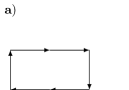
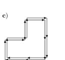
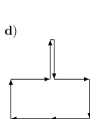
Figure 1: a) For this loop the perimeter $L$ is equal to the number of lattice sites $2n=6$, number of straight sections/sides is $k=4$, and number of windings $I=1$. b) Here, $2n=8$, $k=6$ and $I=1$ (number of winding would not change with orientation of the loop). c) Here, $2n=16$ and $I=2$ and $k=12$. d) Non-allowed loop, since it consists of backtracking.

Next, we parametrize the unit tangent vectors in spherical coordinates as

$$\bm{e}(i)=(\sin\theta_{i}\cos\phi_{i},\sin\theta_{i}\sin\phi_{i},\cos\theta_{i}),$$ (24)

and represent the eigenstates of the vector of Pauli matrices as $|\bm{e}(i);\pm\rangle$, which satisfy,

$$\bm{\gamma}\cdot\bm{e}(i)|\bm{e}(i);\pm\rangle=\pm|\bm{e}(i);\pm\rangle,$$ (25)

implying in this way,

$$\Gamma(\bm{e}(i))=2|\bm{e}(i);-\rangle\langle\bm{e}(i);-|.$$ (26)

Therefore,

$$\text{tr}\bigg{[}\prod^{k}_{i=1}\Gamma(\bm{e}(i))\bigg{]}=2^{k}\prod^{k}_{i=1}\langle\bm{e}(i);-|\bm{e}(i+1);-\rangle$$ (27)

where $|\bm{e}(k+1);-\rangle=|\bm{e}(1);-\rangle$. From now on, we denote $|\bm{e}(i);-\rangle\equiv|\bm{e}(i)\rangle$ for notational simplicity. The inner product can be written in terms of amplitude and phase, as

$$\langle\bm{e}(i)|\bm{e}(i+1)\rangle=|\langle\bm{e}(i)|\bm{e}(i+1)\rangle|\exp(i\arg[\langle\bm{e}(i)|\bm{e}(i+1)\rangle]).$$ (28)

Note that $|\langle\bm{e}(i)|\bm{e}(i+1)\rangle|=\frac{1}{\sqrt{2}}$ for all $i$, which can be seen by simply calculating the magnitude of the inner product between all distinct pairs. For the phase factor we have

$$\arg\langle\bm{e}(i)|\bm{e}(i+1)\rangle =\arctan\bigg{[}\frac{\sin\Delta\phi_{i}\cot\frac{\theta_{i}}{2}\cot\frac{\theta_{i+1}}{2}}{1+\cos{\Delta\phi_{i}}\cot\frac{\theta_{i}}{2}\cot\frac{\theta_{i+1}}{2}}\bigg{]}{}$$

$$=\frac{\Omega_{i}^{\prime}}{2},$$ (29)

where the $\Omega_{i}^{\prime}$ is the area of an spherical triangle on a unit sphere Todhunter (1863), which is shown on Fig. 2 with the corners defined by the unit vectors $-\hat{z}$, $\bm{e}(i)$ and $\bm{e}(i+1)$. Now if we combine Eq. 29 with Eq. 27 we obtain

$$\text{tr}\bigg{[}\prod^{k}_{i=1}\Gamma(\bm{e}(i))\bigg{]} =2^{k/2}\prod^{k}_{i=1}\exp\bigg{(}i\frac{\Omega^{\prime}_{i}}{2}\bigg{)}{}$$

$$=2^{k/2}\exp{i\frac{\Omega^{\prime}}{2}}$$ (30)

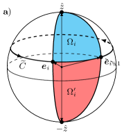
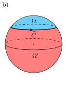
Figure 2: a) For a given $\widetilde{C}$, $\Omega_{i}$ is the solid angle traced by $\bm{e}_{i}$ while travelling from $i$ to $i+1$ b) $\Omega^{\prime}$ is $4\pi-\Omega$.

Note that $\bm{e}$ is a unit tangent to the path $C_{2n}$. Now if we consider a moving frame on path $C_{2n}$, we define $\widetilde{C}$ as the path such that the tip of $\bm{e}$ draws in this moving frame see Fig. 3.

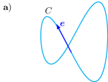
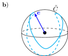
Figure 3: a) Here $C$ is a world line of a fermion and $\bm{e}$ is the unit tangent to $C$. b) $\tilde{C}$ is the curve drawn by the tip of $\bm{e}$ while travelling on $C$.

As it is shown in Fig. 2, if we define $\Omega$ as the total solid angle acquired by $\bm{e}$ while travelling the given loop, then $\Omega^{\prime}=4\pi-\Omega$. This can be better seen if we assume for a moment a continuous case such that $\Delta\phi_{i}\ll 1$ and $\theta_{i}\sim\theta_{i+1}$. In this case we would have

$$\Omega^{\prime}_{i}\sim\Delta\phi_{i}(1+\cos\theta_{i}),$$ (31)

and thus

$$\exp{i\frac{\Omega^{\prime}}{2}} =\exp\bigg{[}{\frac{i}{2}\int_{\widetilde{C}}ds\dot{\phi}(1+\cos{\theta})}\bigg{]}{},$$

$$=\exp(\frac{i}{2}[4\pi-\Omega]){},$$

$$=\exp(-\frac{i}{2}\Omega).$$ (32)

Thus, after Taylor expanding the exponential in Eq. 20, we can express the partition function as,

$$Z=\sum_{N=0}^{\infty}\frac{1}{N!}\prod_{j}^{N}\bigg{[}\sum_{\{C_{j}\}}-2^{L[C_{j}]-k_{j}/2}\frac{\kappa^{L[C_{j}]}}{I_{C_{j}}}e^{-\frac{i}{2}\Omega_{C_{j}}}\bigg{]}$$ (33)

where $\sum_{\{C_{j}\}}$ is summation over all non-back tracing connected loops and $L[C_{j}]$ is the perimeter of the loop, which is simply given by the number of sites on the loop. In Eq. 33 we sum over all possible loops, where some of these loops trace a path several times as it is shown in Fig. 1-c. We can rewrite Eq. 33 in an equivalent form where we sum over loops with single winding as,

$$Z={}$$

$$\sum_{N=0}^{\infty}\frac{1}{N!}\prod_{j}^{N}\bigg{[}\sum_{\{C_{j}\}^{\prime}}\sum_{n_{j}=1}^{\infty}-2^{n_{j}L[C_{j}]-\frac{n_{j}k_{j}}{2}}\frac{\kappa^{n_{j}L[C_{j}]}}{n_{j}}e^{-\frac{i}{2}n_{j}\Omega_{C_{j}}}\bigg{]}$$ (34)

where $\sum_{\{C_{j}\}^{\prime}}$ denotes the sum over loops with single windings and $n_{j}$ is the winding number.

Finally, we can write the solid angle $\Omega$ swept out by $\bm{e}$ in terms of writhe of the curve. To do so we follow the approach of Refs. Grundberg et al. (1989); Frank-Kamenetskiĭ and Vologodskiĭ (1981). Assume that we have a closed curve $C_{1}$ of length $L$ with parametrization $\bm{r}_{1}(s)$ where $0\leq s\leq L$. We also set $s$ as the arc length between $\bm{r}_{1}(0)$ and $\bm{r}_{1}(s)$ of the curve, which implies $|\dot{\bm{r}}_{1}|=1$. Now assume that we have another curve $C_{2}$, with parametrization $\bm{r}_{2}$, such that $\bm{r}_{2}=\bm{r}_{1}+\epsilon\bm{a}$, where $\bm{a}$ is the unit vector normal to $\bm{r}_{1}$ i.e. $\bm{r}_{1}\cdot\bm{a}=0$, and $\epsilon$ is an infinitesimal constant; see Fig. 4.

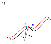
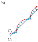
Figure 4: a) Here $\bm{e}$ is the tangent vector at point $\bm{r}_{1}$ on curve $C_{1}$ and $\epsilon\bm{a}$ is the distance between $C_{2}$ and $C_{1}$, where $\bm{a}\cdot\bm{r}_{1}=0$. b) If $C_{2}$ winds around $C_{1}$, $\bm{a}$ rotates around $C_{1}$. If we view $C_{1}$ and $C_{2}$ as edges of a ribbon, then $\bm{a}$ rotates as the ribbon twists. The expression $\frac{\bm{a}\times\bm{\dot{a}}\epsilon^{2}}{\epsilon^{2}}\cdot{\bm{e}}$ can be regarded as the angular speed of the point $\epsilon\bm{a}$ around $\bm{e}$, and the expression for the twist as given in Eq. 35d is the angular displacement of $\epsilon\bm{a}$ divided by $2\pi$.

Now recall the Călugăreanu-White theorem Călugăreanu (1959, 1961); White (1969), which relates and defines the linking number $G$, the writhe $\mathcal{W}$, and the twist $T$ of two curves as Grundberg et al. (1989); Frank-Kamenetskiĭ and Vologodskiĭ (1981),

$$G[C_{1},C_{2}] =\mathcal{W}[C_{1}]+T[C_{1},C_{2}],$$ (35a)

$$G[C_{1},C_{2}] =\frac{1}{4\pi}\oint_{C_{1}}\oint_{C_{2}}\frac{d\bm{r}_{1}\times d\bm{r}_{2}\cdot[\bm{r}_{1}-\bm{r}_{2}]}{|\bm{r}_{1}-\bm{r}_{2}|^{3}},$$ (35b)

$$\mathcal{W}[C_{1}] =\frac{1}{4\pi}\oint_{C_{1}}\oint_{C_{1}}\frac{d\bm{r}_{1}\times d\bm{r}_{2}\cdot[\bm{r}_{1}-\bm{r}_{2}]}{|\bm{r}_{1}-\bm{r}_{2}|^{3}},$$ (35c)

$$T[C_{1},C_{2}] =\frac{1}{2\pi}\int_{0}^{L}ds[\bm{{a}}({s})\times\bm{\dot{a}}({s})]\cdot\bm{\dot{r}}_{1}({s}).$$ (35d)

We now seek to relate the writhe $\mathcal{W}$ to $\Omega$ and proceed by first relating the twist $T$ to $\Omega$ and then use Eq. (35a). Since $|\dot{\bm{r}}_{1}|=1$, $\dot{\bm{r}}_{1}$ is the unit tangent vector to curve $C_{1}$, i.e. $\dot{\bm{r}}_{1}(s)=\bm{e}(s)$, and we parametrize it as $\bm{e}(s)=\hat{\bm{e}}_{r}(s)$, where $\hat{\bm{e}}_{r}(s)$ is a radial unit vector in spherical coordinates as in Eq. 24, and we can choose the frame vector Grundberg et al. (1989) $\bm{a}(s)=\hat{\bm{e}}_{\phi}(s)$ where $\hat{\bm{e}}_{\phi}(s)$ is the azimuthal unit vector in spherical coordinates. We then evaluate Eq. 35d as,

$$T[C_{1},C_{2}] =\frac{1}{2\pi}\oint_{C_{1}}d\bm{r}_{1}\cdot[\bm{{a}}({s})\times\bm{\dot{a}}({s})]{}$$

$$=\frac{1}{2\pi}\int_{0}^{L}ds\dot{\phi}(s)\cos{\theta(s)}.$$ (36)

Next, the solid angle traced by $\hat{\bm{e}}_{r}$ while traveling on $C_{1}$ is given as,

$$\Omega =\oint_{\widetilde{C}_{1}}d\bm{e}_{r}\cdot\hat{\bm{e}}_{\phi}\frac{1-\cos\theta}{|e_{r}|\sin\theta},$$ (37a)

$$=\int_{0}^{L}ds\dot{\phi}(s)(1-\cos{\theta}(s)),$$ (37b)

$$=2\pi u-\int_{0}^{L}ds\dot{\phi}(s)\cos{\theta(s)},\quad u\in\mathbb{Z},$$ (37c)

$$=-2\pi T[C_{1},C_{2}]\mod(2\pi).$$ (37d)

Note that in Eq. 37a we take the line integral over a vector potential of a Dirac monopole along the curve $\widetilde{C}_{1}$, which yields the solid angle associated to $\widetilde{C}_{1}$, which corresponds to the solid angle swept by $\bm{e}$ traveling along $C_{1}$. In Eq. 37c we used the fact that $\bm{r}_{1}(0)=\bm{r}_{1}(L)$. Finally, we substitute Eq. 37d to Eq. 35a to get,

$$\mathcal{W}[C]=\frac{\Omega}{2\pi}+p,$$ (38)

where $p=G-u$. Finally, we can use the observation that $p$ is an odd integer Grundberg et al. (1989).

Now by putting Eq. 38 into Eq. 34 we obtain the exact fermionic partition function as a series in $\kappa$ of the form

$$Z =\sum_{N=0}^{\infty}\frac{1}{N!}\prod_{j}^{N}\bigg{[}\sum_{\{C_{j}\}^{\prime}}\sum_{n_{j}=1}^{\infty}z[C_{j},n_{j}]\bigg{]}$$ (39a)

$$z =-2^{n_{j}L[C_{j}]-\frac{n_{j}k_{j}}{2}}\frac{\kappa^{n_{j}L[C_{j}]}}{n_{j}}(-1)^{n_{j}}e^{-i\pi n_{j}\mathcal{W}[C_{j}]},$$ (39b)

where $C_{j}$ denotes a closed loop with straight sections $k_{j}$, length $L[C_{j}]$, winding number $n_{j}$ and, most importantly, writhe $\mathcal{W}[C_{j}]$.

As a side note, the above result is closely related to the usual loop representation of the fermionic determinant in terms of loops, within a so called the hopping parameter expansion (more details can be found in section 5.1.3 of Ref. Montvay and Münster (1994)).

IV Convergence of the Lattice Fermionic Determinant

The series expansion for the lattice determinant for Wilson fermions above in Eq. 19c raises the question as to its radius of convergence, and in particular the critical value of $\kappa$. For this discussion we adopt the approach of Ref. Gattringer et al. (1999). Since the term in the exponential of Eq. 19c is the series expansion of $\text{Tr}\big{[}\ln\big{[}1-\kappa M\big{]}\big{]}$, the series converges for

$$\kappa||M||_{\infty}<1,$$ (40)

where the infinity norm is given as the square root of the largest eigenvalue of the $M^{\dagger}M$ Gattringer et al. (1999). In order to find it, we first use the Fourier representation of $M$,

$$M_{nm} =\sum_{\mu}\int_{-\pi}^{\pi}\frac{d^{3}p}{(2\pi)^{3}}e^{ip(n-m)}2[\cos(p_{\mu})-i\gamma_{\mu}\sin(p_{\mu})]{}$$

$$=\int_{-\pi}^{\pi}\frac{d^{3}p}{(2\pi)^{3}}e^{ip(n-m)}\sum_{\alpha=\pm}|\alpha\rangle\langle\alpha|E_{\alpha}(p)$$ (41)

where in the last line we write $M$ in a diagonal form using the eigenvectors $|\alpha\rangle$ of $M_{nm}$, and $E_{\pm}(p)=2\big{[}\sum_{\mu}\cos(p_{\mu})\pm i[\sum_{\mu}\sin^{2}(p_{\mu})]^{1/2}\big{]}$. Thus, we can Fourier transform $M^{\dagger}M$ as

$$(M^{\dagger}M)_{nm}=\int_{-\pi}^{\pi}\frac{d^{3}p}{(2\pi)^{3}}e^{ip(n-m)}\sum_{\alpha}|\alpha\rangle\langle\alpha||E_{\alpha}(p)|^{2}$$ (42)

where $|E(p)|^{2}=4\big{[}[\sum_{\mu}\cos(p_{\mu})]^{2}+\sum_{\mu}\sin^{2}(p_{\mu})\big{]}$. Thus $|E(0)|^{2}=36$ is the highest eigenvalue and the norm is $||M||_{\infty}=6.$ We parametrize $\kappa$ as

$$\kappa=\frac{1}{6}e^{-m}$$ (43)

where $m=\ln(1+\frac{m_{0}}{3})$ then using Eq. 40 we find that the series converges for $m_{0}>0$. Thus not surprisingly, we find that the series converges only for a nonzero bare mass. We can now rewrite Eq. 39a using Eq. 43 as,

$$Z =\sum_{N=0}^{\infty}\frac{1}{N!}\prod_{j}^{N}\bigg{(}\sum_{\{C_{j}\}^{\prime}}\sum_{n_{j}=1}^{\infty}z[C_{j},n_{j}]\bigg{)}.$$ (44a)

$$z =-\frac{2^{L[C_{j}]n_{j}-n_{j}k_{j}[C_{j}]/2}}{6^{n_{j}L[C_{j}]}}\frac{(-1)^{n_{j}}}{n_{j}}e^{-mn_{j}L[C_{j}]}e^{-i\pi n_{j}\mathcal{W}[C_{j}]}.$$ (44b)

This final form of the fermionic partition sum expressed in terms of the writhe is our first key result.

V Particle-vortex duality in the Chern-Simons lattice Abelian Higgs model

Having studied the bosonic continuum actions of Eqs. (2) in Sec. II, and given form of the partition sum of the fermionic action in terms of the writhe derived in the last section, we aim to establish the bosonization duality between the lattice versions of Eqs. (2) and (3) by also expressing the bosonic partition sum in terms of the writhe. We proceed in three steps: first, we connect the bosonic particle-vortex duality in the continuum to its lattice equivalent, then calculate the bosonic partition sum in the dual bosonic action, and finally compare it with the fermionic result.

V.1 Particle-vortex duality on the lattice

The partition function for the Abelian CS Higgs model on the lattice with a non-compact gauge field is given by,

$$Z=\left[\prod_{j,\mu}\int_{0}^{2\pi}\frac{d\varphi_{j}}{2\pi}\int_{-\infty}^{\infty}da_{j\mu}\right]\sum_{\{n_{j\mu}\}}e^{-S},$$ (45)

where the lattice action is given in the Villain approximation as,

$$S = \sum_{j}\left[i\frac{\theta}{4\pi^{2}}\epsilon_{\mu\nu\lambda}a_{j\mu}\Delta_{\nu}a_{j\nu}\right.$$

$$+ \left.\frac{J}{2}(\Delta_{\mu}\varphi_{j}-2\pi n_{j\mu}-a_{j\mu})^{2}\right],$$

where $\sum_{\{n_{i\mu}\}}=\prod_{i\mu}\sum_{n_{i\mu}=-\infty}^{\infty}$, $J>0$ is the bare phase stiffness and $\Delta_{\mu}$ represents the forward discrete derivative, $\Delta_{\mu}f_{i}=f_{i+1}-f_{i}$. In the above action the integer valued lattice fields $n_{j\mu}$ enforces the periodicity of $\varphi_{j}$ fulfilling the integer (or vortex) gauge invariance, $\varphi_{j}\to\varphi_{j}+2\pi L_{j\mu}$, $n_{j\mu}\to n_{j\mu}+L_{j\mu}$, where $L_{j\mu}$ is an arbitrary integer. This discrete gauge invariance is a common feature of the so called Villain action Kleinert (1989) and arises here in addition to the usual gauge invariance associated to the lattice gauge field $a_{j\mu}$.

In order to derive the dual model, we follow closely the approach of Ref. Peskin (1978) and use the Poisson summation formula,

$$(2\pi a)^{1/2}\sum_{n=-\infty}^{\infty}e^{-\frac{a}{2}(x-2\pi n)^{2}}$$ (47)

$$= \sum_{m=-\infty}^{\infty}e^{-\frac{1}{2a}m^{2}+ixm},$$

to introduce an auxiliary integer-valued lattice field $J_{j\mu}$, i.e.,

$$\sum_{\{n_{j\mu}\}}e^{-\frac{J}{2}(\Delta_{\mu}\varphi_{j}-2\pi n_{j\mu}-a_{j\mu})^{2}}$$ (48)

$$\sim \sum_{\{J_{j\mu}\}}e^{-\frac{1}{2J}J_{j\mu}^{2}+iJ_{j\mu}(a_{j\mu}-\Delta_{\mu}\varphi_{j})}.$$

Next we use summation by parts in the term $-J_{j\mu}\Delta_{\mu}\varphi_{j}$ to convert it to $\Delta_{\mu}J_{j\mu}\varphi_{j}$, which allows us to integrate the phase variables out to obtain the zero divergence constraint, $\Delta_{\mu}J_{j\mu}=0$. The latter implies that we are dealing with a sum over configurations where the vortices form loops Kleinert (1989). The action is thus rewritten as

$$S^{\prime}=\sum_{j}\left[i\frac{\theta}{4\pi^{2}}\epsilon_{\mu\nu\lambda}a_{j\mu}\Delta_{\nu}a_{j\nu}+\frac{1}{2J}J_{j\mu}^{2}-iJ_{j\mu}a_{j\mu}.\right].$$ (49)

The constraint is solved by introducing the curl of another integer field, $M_{j\mu}$, such that $J_{j\mu}=\epsilon_{\mu\nu\lambda}\Delta_{\nu}M_{j\lambda}$, which leads to,

$$S^{\prime\prime} = \sum_{j}\left[i\frac{\theta}{4\pi^{2}}\epsilon_{\mu\nu\lambda}a_{j\mu}\Delta_{\nu}a_{j\nu}+\frac{1}{2J}(\epsilon_{\mu\nu\lambda}\Delta_{\nu}M_{j\lambda})^{2}\right.$$ (50)

$$- \left.i(\epsilon_{\mu\nu\lambda}\Delta_{\nu}M_{j\lambda})a_{j\mu}\right].$$

Thus, upon integrating out the gauge field $a_{j\mu}$, we obtain,

$$Z = \sum_{\{M_{j\mu}\}}e^{-S^{\prime\prime\prime}}$$

$$S^{\prime\prime\prime} = \frac{1}{2}\sum_{j}\left[\frac{1}{J}(\epsilon_{\mu\nu\lambda}\Delta_{\nu}M_{j\lambda})^{2}-i\frac{2\pi^{2}}{\theta}\epsilon_{\mu\nu\lambda}M_{j\mu}\Delta_{\nu}M_{j\lambda}\right].$$

We now use the Poisson summation formula in the form,

$$\sum_{n=-\infty}^{\infty}f(n)=\sum_{m=-\infty}^{\infty}\int_{-\infty}^{\infty}\frac{dk}{2\pi}e^{i2\pi km}f(k),$$ (52)

to convert the integer field $M_{j\mu}$ into a real-valued gauge field $b_{j\mu}$, and noting that this last step introduces another integer field $\widetilde{J}_{j\mu}$, we obtain finally the dual action in the form

$$\widetilde{S} = \frac{1}{2}\sum_{j}\left[\frac{1}{J}(\epsilon_{\mu\nu\lambda}\Delta_{\nu}b_{j\lambda})^{2}-i\frac{2\pi^{2}}{\theta}\epsilon_{\mu\nu\lambda}b_{j\mu}\Delta_{\nu}b_{j\lambda}\right]$$ (53)

$$- i2\pi\sum_{j}\widetilde{J}_{j\mu}b_{j\mu},$$

after integrating out $a_{j\mu}$. Note that unlike the original action (V.1), the dual action above features a Maxwell term with the bare phase stiffness of the original model appearing as a gauge coupling. As a consequence of gauge invariance, the lattice vortex current field $\widetilde{J}_{j\mu}$ also has a vanishing divergence.

By letting $J\to\infty$ in Eq. (53), we see that for $\theta=\pi$ and after rescaling $b_{j\mu}\to b_{j\mu}/(2\pi)$ the latter is the same as the one arising in the partition function (49) up to the sign of the CS term. As far as the partition function is concerned, the sign of the CS term is immaterial, since integrating out either $a_{j\mu}$ or $b_{j\mu}$ in the $J\to\infty$ limit leads to the same vortex current interaction when $\theta=\pi$ as we sum over all integer-valued vortex currents. The theory is thus self-dual in this regime.

If we smear the constraint $\Delta_{\mu}\widetilde{J}_{j\mu}=0$ by adding the term $(\gamma/2)\widetilde{J}_{j\mu}^{2}$ to the dual action (53), corresponding to adding a chemical potential for the vortex loops Peskin (1978); Dasgupta and Halperin (1981), and apply once more the Poisson formula (47), we obtain,

$$\widetilde{S}^{\prime} = \frac{1}{2}\sum_{j}\left[\frac{1}{J}(\epsilon_{\mu\nu\lambda}\Delta_{\nu}b_{j\lambda})^{2}-i\frac{2\pi^{2}}{\theta}\epsilon_{\mu\nu\lambda}b_{j\mu}\Delta_{\nu}b_{j\lambda}\right.$$ (54)

$$+ \left.\frac{1}{\gamma}(\Delta_{\mu}\widetilde{\varphi}_{j}-2\pi N_{j\mu}-2\pi b_{j\mu})^{2}\right],$$

where $N_{j\mu}$ is an integer lattice field and $\widetilde{\varphi}_{j}$ is a phase variable originating from the integral representation of the Kronecker delta constraint enforcing $\Delta_{\mu}\widetilde{J}_{j\mu}=0$, i.e.,

$$\delta_{\Delta_{\mu}\widetilde{J}_{j\mu},0}=\int_{-\pi}^{\pi}\frac{d\widetilde{\varphi}_{j}}{2\pi}e^{i\widetilde{\varphi}_{j}\Delta_{\mu}\widetilde{J}_{j\mu}}.$$ (55)

Equation (10), equation (V.1) and its dual form in Eq. (54) establishes a lattice version of the field theory duality of Eq. (2) in the regime where amplitude fluctuations of the bosonic fields are neglibile. The continuum limit of the lattice duality is expected to approach the field theory duality in the vicinity of the critical point. However, we should emphasize that precise statements to this effect can only be achieved within the lattice formalism.

V.2 Duality and writhe

In the case of the partition function for Wilson fermions we have seen that in order to make the writhe more apparent we had to partially evoke a continuum limit, while still counting fermionic loops configurations. We will employ a similar strategy for the dual bosonic partition function (53) in order to express it terms of linking and writhe numbers. Thus, the continuum version of (53) can be obtained by first writing a functional integral for a given configuration featuring $N$ vortex loops,

$$Z \propto\sum_{\{\widetilde{J}_{x\mu}\}}{}^{{}^{\prime}}\int\mathcal{D}be^{-S_{\text{MCS}}}$$ (56a)

$$S_{\rm MCS} =\int d^{3}x\left[\frac{1}{2J}(\epsilon_{\mu\nu\lambda}\partial_{\nu}b_{\lambda})^{2}\right.$$

$$-\left.\frac{i\pi^{2}}{\theta}\epsilon_{\mu\nu\lambda}b_{\mu}\partial_{\nu}b_{\lambda}-i2\pi\widetilde{J}_{\mu}b_{\mu}\right],$$ (56b)

with,

$$\widetilde{J}_{\mu}(x)=\sum_{a=1}^{N}n_{a}\int_{0}^{\tilde{L}_{a}}ds\frac{dy_{\mu}^{a}(s)}{ds}\delta^{3}(x-y^{a}(s)),$$ (57)

where, $n_{a}\in\mathbb{Z}^{+}$ is the quantum number of the $a$-th vortex loop and $y_{\mu}^{a}(s)$, $s\in[0,\tilde{L}_{a}]$ is a parametrization of the curve describing a loop $C_{a}$ with length $\tilde{L}_{a}$ satisfying the boundary conditions $y_{\mu}^{a}(0)=y_{\mu}^{a}(\tilde{L}_{a})$. Equation (57) clearly satisfies $\partial_{\mu}\widetilde{J}_{\mu}=0$.

We can write the partition function as a summation over all possible vortex current fields $\widetilde{J}$ configurations as;

$$Z=\sum_{N=0}^{\infty}\frac{1}{N!}\prod_{j=1}^{N}\sum_{\{C_{j}\}^{\prime}}\sum_{n_{j}}Z(C_{1},n_{1};\dots;C_{N},n_{N})$$ (58)

where $Z(C_{1},n_{1};\dots;C_{N},n_{N})$ is a partition function with a fixed vortex configuration which consists of $N$ number of vortex loops, where the $a$-th loop has a shape $C_{a}$ and vortex quantum number $n_{a}$. Multiplication by $\frac{1}{N!}$ provides the symmetry factor preventing the overcounting of identical configurations, and $\sum_{\{C\}^{\prime}}$ is summation over all connected non-backtracing loops with single winding and with both orientations. Explicitly we can write the partition function for a fixed configuration as,

$$Z(C_{1},n_{1};\dots;C_{N},n_{N})=\int\mathcal{D}b_{\mu}e^{-S_{\rm MCS}},$$ (59)

normalized such that $Z(0)=1$. We now integrate out $b_{\mu}$, in momentum space so that

$$Z(C_{1},n_{1};\dots;C_{N},n_{N})=$$

$$\exp\left[-2\pi^{2}\int\frac{d^{3}p}{(2\pi)^{3}}D_{\mu\nu}(p)\widetilde{J}_{\mu}(p)\widetilde{J}_{\nu}(-p)\right],$$ (60)

where,

$$D_{\mu\nu}(p) = \frac{J}{p^{2}+4\pi^{4}J^{2}/\theta^{2}}\left(\delta_{\mu\nu}-\frac{p_{\mu}p_{\nu}}{p^{2}}\right.$$ (61)

$$- \left.\frac{2\pi^{2}J}{\theta}\frac{\epsilon_{\mu\nu\lambda}p_{\lambda}}{p^{2}}\right),$$

in the Landau gauge. Equation (V.2) give a vortex interaction identical to the one in Eq. (11) when $\rho$ is uniform.

In the limit where $J\to\infty$, which corresponds to $\Lambda\to\infty$ in the case ot $\rho_{0}$, we obtain

$$Z(C_{1},n_{1};\dots;C_{N},n_{N})=$$

$$\exp\left[\frac{i\theta}{4\pi}\sum_{a,b}n_{a}n_{b}\oint_{C_{a}}\oint_{C_{b}}dy_{\mu}^{a}dy_{\nu}^{b}\frac{\epsilon_{\mu\nu\lambda}(y_{\lambda}^{a}-y_{\lambda}^{b})}{|y^{a}-y^{b}|^{3}}\right],$$ (62)

which in view of Eq. 35 can be rewritten as

$$Z(\{C\})={}$$

$$\exp\left(i\theta\sum_{a}n_{a}^{2}\mathcal{W}[C_{a}]+i2\theta\sum_{a<b}n_{a}n_{b}G_{ab}\right),$$ (63)

where we have introduced the notation, $\{C\}=\{C_{1},n_{1};\dots;C_{N},n_{N}\}$. For $\theta=\pi$ the term proportional to $G_{ab}$ does not contribute to the partition function due to the Gauss linking number theorem. If we use a statistical mechanical language and interpret $J$ as the exchange energy divided by the temperature and refer to the original lattice action (V.1), we see that the limit $J\to\infty$ corresponds to a zero temperature limit in this context. Furthermore, $J$ is related to the amplitude of the scalar field $\phi$, such that $J\sim\rho_{0}^{2}$, and we have seen in Section II that $\rho_{0}^{2}$ is indeed very large. Peskin Peskin (1978) in his analysis of the particle-vortex duality referred to this regime as a ”frozen superconductor”. The analysis in Ref. Peskin (1978) ignores the vortex core energy and adds it by hand as a small chemical potential for the vortices Peskin (1978); Dasgupta and Halperin (1981). However, the vortex core energy arises quite naturally, since it is related to the correlation length in the continuum theory. Furthermore, there is a direct relation between it and the bare mass, as we discussed in Section II. Therefore, the actual result corresponding to large $J$ is given by

$$Z(\{C\})={}$$

$$\exp\left(i\theta\sum_{a}n_{a}^{2}\mathcal{W}[C_{a}]+i2\theta\sum_{a<b}n_{a}n_{b}G_{ab}-\epsilon\sum_{a}n_{a}^{2}\tilde{L}_{a}\right).$$ (64)

where $\epsilon$ is the vortex core energy given by Eq. (15). As in Eq. (V.2), for $\theta=\pi$ the second term does not contribute, since $G_{ab}\in\mathbb{Z}$ by virtue of the Gauss linking number theorem. Thus, after summing over all loop configurations we obtain the partition function as

$$Z=\sum_{N=0}^{\infty}\frac{1}{N!}\prod_{j=1}^{N}\sum_{\{C_{j}\}}\sum_{n_{j}}\bigg{[}\exp(i\pi\mathcal{W}[C_{j}])\exp(-\epsilon\tilde{L}[C_{j}])\bigg{]}^{n_{j}^{2}},$$ (65)

an equation that has the same form as Eq. (16), with $S_{\rm vortex}=-i\pi\mathcal{W}$. The factor $\exp(i\pi\mathcal{W}[C_{j}])$ is crucial for the fermion-boson transmutation in 2+1 dimensions and is referred to as a ”spin factor” in the literature Ambjørn et al. (1990); Grundberg et al. (1990); Goldman and Fradkin (2018).

VI Comparison of fermionic and bosonic partition functions

Let us now compare the fermionic partition function with the bosonic one in the continuum. In order to take the continuum limit of lattice fermionic partition function, we first return to Eq. 27 and introduce the lattice spacing explicitly,

$$\text{tr}[M_{C_{2n}}] =\text{tr}\bigg{[}\prod^{2n}_{j=1}\Gamma(\bm{e}(ja))\bigg{]}=\prod^{2n}_{j=1}2\langle\bm{e}(ja)|\bm{e}((j+1)a)\rangle{}$$

$$=\prod^{2n}_{j=1}2\bigg{[}1+a\langle\bm{e}(s)|\frac{d}{ds}\bm{e}(s)\rangle\big{|}_{s=ja}+\mathcal{O}(a^{2})\bigg{]}{}$$

$$=\prod^{2n}_{j=1}2\bigg{[}1+\frac{i}{2}a\dot{\phi}(s)(1+\cos(\theta(s)))+\mathcal{O}(a^{2})\bigg{]}{}$$

$$\sim 2^{\frac{\tilde{L}}{a}}\exp{-\frac{i}{2}\Omega[C_{\tilde{L}}]}$$ (66)

where $\tilde{L}[C]=aL[C]$ and in the last line we used Eq. 32. In this case Eq. 44 becomes,

$$Z =\sum_{N=0}^{\infty}\frac{1}{N!}\prod_{j}^{N}\bigg{[}\sum_{\{C_{j}\}^{\prime}}\sum_{n_{j}=1}^{\infty}z[C_{j},n_{j}]\bigg{]}$$ (67a)

$$z =-{2^{\widetilde{L}[C_{j}]n_{j}/a}}e^{-i\pi n_{j}W[C_{j}]-(m+\ln 6)\widetilde{L}[C_{j}]n_{j}/a}\frac{(-1)^{n_{j}}}{n_{j}}.$$ (67b)

We confine ourselves to the low-energy sector corresponding to $n_{j}=1$, in which case the fermionic partition function becomes,

$$Z_{F}=\sum_{N=0}^{\infty}\frac{1}{N!}\prod_{j=1}^{N}\sum_{\{C_{j}\}}{2^{\widetilde{L}[C_{j}]/a}}e^{-i\pi W[C_{j}]-(m+\ln 6)\widetilde{L}[C_{j}]/a}.$$ (68)

In the limit $m_{0}a\ll 1$, we have $m=\ln(1+m_{0}a/3)\approx m_{0}a/3$, which implies,

$$Z_{F}\propto\sum_{N=0}^{\infty}\frac{1}{N!}\prod_{j=1}^{N}\sum_{\{C_{j}\}}e^{-i\pi W(C_{j})-\widetilde{M}_{0}\tilde{L}(C_{j})},$$ (69)

where

$$\widetilde{M}_{0}=\frac{m_{0}}{3}+\frac{1}{a}\ln 3.$$ (70)

The key observation is that the bosonic partition function Eq. 65

$$\epsilon=\widetilde{M}_{0}=\frac{m_{0}}{3}+\frac{1}{a}\ln 3.$$ (71)

It is possible to connect this result to the continuum theory via the ensemble of paths discussed in Section Section II. Accordingly, by using Eq. (15), we obtain a relation between the fermion, the boson mass $m_{B}$ and the $|\phi|^{4}$ coupling $\lambda$ of the continuum model,

$$\frac{m_{0}a}{3}=\frac{a^{2}}{6}\left(m_{B}^{2}+\frac{3\lambda}{2}\rho_{0}^{2}\right)+\ln 2.$$ (72)

Thus, we have found that in the regime where the vortex energy entering the Boltzmann weight is minimum, corresponding to the winding $n_{j}=1$ in Eq. 65 , the latter is identical to the fermionic partition function where in the fermion loop worldlines the particle travels the loop only once. This establishes a correspondence between the fermionic particle worldline loops and vortex loops in the bosonic dual CS theory, which in turn sheds new light on Polyakov’s result for a first-quantized path integral description of massive Dirac fermions in 2+1 dimensions Polyakov (1988).

VII Discussion

The duality transformation from the Villain action (V.1) to (54) identifies in the continuum limit to the duality (2). In contrast to the situation in 3+1 dimensions, the Maxwell term is IR irrelevant in 2+1 dimensions, and therefore both theories in (2) flow to the same gauged (IR stable) Wilson-Fisher fixed point. This situation corresponds in the lattice to $J$ large compared to the momentum scale. In the field theory we identify $e^{2}=J$. The renormalization of $e^{2}$ can be obtained as usual from the parity-even contribution to the vacuum polarization, $\Pi(p)$. Thus, the renormalized gauge coupling is given simply by,

$$e_{R}^{2}=\frac{e^{2}}{1+e^{2}\Pi(0)}.$$ (73)

Gauge invariance implies that $\Pi(0)=k/\widehat{m}_{R}$, where $k$ is some universal constant. Therefore, for $e^{2}\to\infty$ we obtain that $e_{R}^{2}\approx\widetilde{m}_{R}/k$. Equivalently, keeping $e^{2}$ fixed and approaching the critical point, $\widetilde{m}_{R}\to 0$ yields the same scaling behavior, leading once more to $e_{R}^{2}\approx\widetilde{m}_{R}/k$. Since $e^{2}$ is identified by the duality as the bare phase stiffness, the scaling behavior $e_{R}^{2}\approx\widetilde{m}_{R}/k$ corresponds precisely to the Josepshon scaling relation Josephson (1966). At the same time we expect that the dimensionless renormalized coupling $\widetilde{\lambda}_{R}/\widetilde{m}_{R}$ approaches the (gauged) Wilson-Fisher fixed point as $\widetilde{m}_{R}\to 0$.

What does the above picture imply for the Dirac fermions? It is usually conjectured that $m_{B}^{2}=0$ implies $m_{0}=0$ Chen et al. (2018); Seiberg et al. (2016); Karch and Tong (2016). Inserting this into Eq. (72) yields at lowest order based on the mean-field result (9),

$$\frac{m_{0}a}{3}=\ln 2,$$ (74)

which clearly never vanishes. However, it is important to realize that the actual critical point corresponds to $m_{R}=0$, which is in general not attained for $m_{B}^{2}=0$. Furthermore, a more accurate picture should relate $m_{0}$ to the phase stiffness beyond the one-loop result. But then other complications may arise, as the fermions will presumably not be in the free theory regime any longer.

VIII Conclusion

In Section V we performed in the lattice an exact duality transformation mapping the partition function of bosons in the ACSH model to the partition function for an ensemble of closed vortex loop excitations of the same model, which corresponds in field theory language to the correspondence shown in the first two lines of the above equation. Furthermore, in Section VI we were able to identify the partition function for an ensemble of vortex loops of the ACSH model in the low-energy regime to the partition function for an ensemble of closed fermion worldlines.

More precisely, we have studied in this work the correspondence between the ACSH model and free massive fermions within the framework of a particle-vortex duality. This was achieved via an exact duality transformation where closed worldline of bosonic particles arising in the partition function of the ACSH model are brought to an equivalent form summing over an ensemble of closed vortex loops of the same model. Thanks to the CS term in the action, this standard particle-vortex duality features a phase factor in the partition function where the phase is given by the writhe number of a pair of vortex loops. We then showed that the fermionic partition function represented as a sum over an ensemble of closed paths of fermionic particles features exactly the same phase factor involving the writhe. In this case the match between the fermionic and bosonic partition functions is established in the low-energy regime where the mass of the fermions is naturally related to the vortex core energy. It turns out that the latter also corresponds to the energy density per element of the path of the bosons in the particle representation of the partition function.

Various aspects of this bosonization duality have been studied intensely in the past, providing conjectures as well as exact results in several limiting cases. Our calculation focus on the self-dual point $\theta=\pi$ of the particle-vortex duality of the ACSH model, and provides exact duality mappings for the lattice versions of Eqs. (2) and (3). We find that the bosonization duality holds for $\theta=\pi$ because the Gauss linking number contributions are then suppressed from the bosonic partition function, leaving only the writhe number contribution. Concretely, the bosonic dual partition function takes the form of a sum over all possible vortex loops with a given writhe yielding the phase factor mentioned above.