: Neural Type Hints

Abstract.

Type inference over partial contexts in dynamically typed languages is challenging. In this work, we present a graph neural network model that predicts types by probabilistically reasoning over a program’s structure, names, and patterns. The network uses deep similarity learning to learn a $\mathit{TypeSpace}$— a continuous relaxation of the discrete space of types — and how to embed the type properties of a symbol (i.e. identifier) into it. Importantly, our model can employ one-shot learning to predict an open vocabulary of types, including rare and user-defined ones. We realise our approach in for Python that combines the $\mathit{TypeSpace}$ with an optional type checker. We show that accurately predicts types. confidently predicts types for 70% of all annotatable symbols; when it predicts a type, that type optionally type checks 95% of the time. can also find incorrect type annotations; two important and popular open source libraries, fairseq and allennlp, accepted our pull requests that fixed the annotation errors discovered.

1. Introduction

Automatic reasoning over partial contexts is critical, since software development necessarily involves moving code from an incomplete state — relative to the specification — to a complete state. It facilitates scaling analyses to large, industrial code bases. For example, it allows quickly building a file-specific call graph when editing a single file instead of requiring a project-level call graph. Traditional static analyses tackle partial contexts via abstraction. They achieve soundness (or soundiness (Livshits et al., 2015)) at the cost of imprecision. As the target language becomes more dynamic (Richards et al., 2010) (e.g. reflection or eval), analysis precision tends to deteriorate.

Optional type systems (Bracha, 2004) feature omittable type annotations that have no runtime effects; they permit reasoning about the types over a partial program that does not contain enough information to be fully typed. In the limit, optional typing reaches traditional static typing when all types are annotated or can be inferred. Recent years have witnessed growing support of optional typing in dynamically typed languages. Notable examples include flow for JavaScript and mypy for Python. This trend indicates that the dynamic typing community increasingly acknowledges the benefits of types, such as early bug detection (Gao et al., 2017), better performance, and accurate code completion and navigation.

Optional typing, however, comes with a cost. Developers who wish to use it need to migrate an unannotated codebase to an (at least partially) annotated one. When the codebase is large, manually adding type annotations is a monumental effort. Type inference can automatically and statically determine the most general type of a program expression, but it offers little help here, because it cannot soundly deduce the types of many expressions in a dynamic language, like JavaScript or Python.

In this work, we present , a machine learning approach that suggests type predictions to a developer. Developers introduce a rich set of patterns into source code, including the natural language elements, such as variable names, and structural idioms in a program’s control and data flows. exploits these noisy and uncertain data, which traditional analysis ignores or conservatively abstracts, to probabilistically suggest types. Any suggestions the developer accepts increase the number of typed terms in a program and enhance the reasoning power of optional typing. Our goal is to help developers move to fully typed programs and return to the safe haven of the guarantees that traditional static typing affords. Our work rests on the idea that verifying a type suggestion helps a developer more quickly find the correct type than coming up with the correct type from scratch.

Research has shown that machine learning methods can effectively predict types (Raychev et al., 2015; Hellendoorn et al., 2018). This pioneering work, however, treats this task as a classification problem and, therefore, have a fixed set of categories, or types in our setting. In other words, they target a closed type vocabulary. However, the types in our corpus generally follow a fat-tailed Zipfian distribution and 32% of them are rare (Sec. 6). Type prediction for closed type vocabularies does not handle rare types and, thus, faces a performance ceiling.

advances the state of the art by formulating probabilistic type inference as a metric-based meta-learning problem, instead of a classification problem. Meta-learning (or “learning-to-learn”) allows trained machine learning models to adapt to new settings with just a single example and no additional training. Metric-based meta-learning models learn to embed a (possibly) discrete input into a real $D$-dimensional latent space preserving its properties. Specifically, learns to embed symbols (identifiers like variable names, parameter names, function names etc.) capturing their type properties. We call these embeddings type embeddings. strives to preserve the type equality relations among type embeddings and establish, through training, a $\mathit{TypeSpace}$ that keeps the type embeddings of symbols that share a type close and those of different types apart. predicts types for identifiers that lack type annotations because they cannot be inferred and have not been provided, so it does not explicitly embed type annotations.

In contrast to classification-based methods, can efficiently predict types unseen during training. Once we have a trained model, we can use it to compute $\boldsymbol{r}\!_{s}$, the type embedding of the symbol $s$ of a new type $\tau$ in the $\mathit{TypeSpace}$. maintains a type map from representative embeddings to their type. This type map implicitly defines “typed” regions in the $\mathit{TypeSpace}$. To allow to predict $\tau$, we update this type map with $\boldsymbol{r}\!_{s}\mapsto\tau$. Now can predict type $\tau$ for symbols whose embeddings fall into a neighbourhood around $\boldsymbol{r}\!_{s}$ in its $\mathit{TypeSpace}$. Thus, can support an open type vocabulary, without retraining. To bootstrap the process, we seed the $\mathit{TypeSpace}$ and the type map with the type embeddings of symbols with known types. A type checker removes false positives. Our results show that makes a substantial advance, improving the state-of-the-art from 4.1% to 22.4%, when predicting an exact match for rare types.

We realise in a graph neural network (GNN). Most existing neural approaches treat programs as sequences of tokens, missing the opportunity to model and learn from the complex dependencies among the tokens in a program. Our experiment reveals that using a graph-based model, instead of a sequence-based model, produces 7.6% more exact matches for common types (Table 2). We implement to predict types for variables, parameters, and function returns in a Python program. For a given symbol, two types are neutral under an optional type system when replacing one with the other does not yield a type error. We show that, given an appropriate confidence threshold that allows each model to predict types for 70% of the symbols in our corpus, ’ predictions achieve type neutrality with the human-provided ones 95% of the time, compared to 60% for the baseline model.

Human-written optional type annotations can fail to trigger a type error even when they are incorrect. can find these errors. In PyTorch/fairseq, a popular sequence-to-sequence modelling toolkit, predicted int when the existing annotation was float; in allenai/allennlp, a popular natural language processing library, predicted Dict[str,ADT] when the existing annotation was ADT. We submitted two pull requests for these errors; both were accepted (Sec. 7). and the evaluation artefacts can be found at https://github.com/typilus/typilus.

Contributions

1. We adapt a graph-based deep neural network to the type prediction problem by considering source code syntax and semantics;

2. We use a novel training loss — based on deep similarity learning — to train a model that embeds the type properties of symbols into a $\mathit{TypeSpace}$ and is adaptive: without retraining, it can accurately predict types that were rare, or even unseen, during training;

3. We realise our approach in for Python and demonstrate its effectiveness in predicting types in an extensive evaluation.

2. Overview

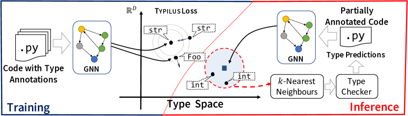
Figure 1. Overview of . Training (left, blue): A graph neural network (GNN) learns to map variables, parameters, and function returns to a type embedding in an $\mathbb{R}^{D}$ type space using deep similarity learning. Inference (right, red): Using the type map, accepts unannotated code, computes type embeddings with the trained GNN and finds the concrete $k$ nearest neighbours types as the candidate predictions. Finally, a type checker checks all predictions and filters incorrect ones.

In this work, we aim to predict types for symbols in an optionally typed language. This task takes two forms, open or closed, depending on whether one aims to predict from a set of types that is finite and closed or unbounded and open. Early work for this task has targeted a closed type vocabulary; DeepTyper considers 11.8k types found in a large TypeScript corpus where JSNice considers a smaller set (Raychev et al., 2015; Hellendoorn et al., 2018). However, most real-life code introduces new, domain-specific types. In our data (Sec. 6), only 158 types (out of 49k) appear more than 100 times, following a Zipfian distribution, similar to other code artefacts (Allamanis and Sutton, 2013). Nevertheless, given the fat-tailed distribution of types, about 32% of the type annotations are rare in our corpus. Thus, predicting from a closed type vocabulary faces a performance ceiling.

We present , a method targeting an open type vocabulary that can predict types unseen during training. Sec. 6 shows that many of these predictions are useful because an type checker can efficiently verify them; when they are not type checkable, we hope they at least speed a developer’s selection of the correct type. Fig. 1 depicts the high-level architecture of .

Learning a Type Space (Fig. 1, left, blue) Central to is its $\mathit{TypeSpace}$, a continuous projection of the type context and properties of code elements into a real multidimensional space. We do not explicitly design this space, but instead learn it from data. To achieve this, we train a neural network $e(\cdot)$ that takes a code snippet $S$ and learns to map the variables, parameters and functions of $S$ into the $\mathit{TypeSpace}$. For each symbol $s\in S$, $e(S)[s]=\boldsymbol{r}\!_{s}\in\mathbb{R}^{D}$. uses deep similarity learning, which needs sets of positive and negative examples for training. To define these sets, we leverage existing type annotations in Python programs: like str and Foo in Fig. 1. To capture both semantic and lexical properties of code, employs a graph neural network (GNN). The GNN learns and integrates information from multiple sources, including identifiers, syntactic constraints, syntactic patterns, and semantic properties like control and data flow.

Predicting Types (Fig. 1, right, red) ’s $e$ alone cannot directly predict a type, since it maps symbols to their type embeddings in $\mathbb{R}^{D}$. Instead, its output, the $\mathit{TypeSpace}$, acts as an intermediate representation between a program’s symbols and their concrete types. To make type predictions, builds $\tau\mathit{map}$ to map a symbol’s type embedding to its type. This implicitly maps each type to a set of type embeddings. First, given a corpus of code — not necessarily the training corpus — we map all known type annotations $\tau_{i}$ into points in the $\mathit{TypeSpace}$. In Fig. 1, int is an example $\tau_{i}$. Given the $\tau\mathit{map}$ and a query symbol $s_{q}$ (the black square in Fig. 1), whose type properties $e$ embeds at $\boldsymbol{r}\!_{s_{q}}$ (i.e. $e(S)[s_{q}]=\boldsymbol{r}\!_{s_{q}}$), returns a probability distribution over candidate type predictions in the neighbour around $\boldsymbol{r}\!_{s_{q}}$ in the $\mathit{TypeSpace}$. uses $k$ nearest neighbours to define this neighbourhood. Finally, a type checker checks the highest-probability type predictions and, if no type errors are found, suggests them to the developer.

Key Aspects

The key aspects of are

• A graph-based deep neural network that learns from the rich set of patterns and can predict types without the need to have a fully resolved type environment.

• The ability to embed the type properties of any symbol, including symbols whose types were unseen during training, thereby tackling the problem of type prediction for an open vocabulary.

• A type checking module that filters false positive type predictions, returning only type-correct predictions.

3. Background

Machine learning has been recently used for predicting type annotations in dynamic languages. Although traditional type inference is a well-studied problem, commonly it cannot handle uncertainty as soundness is an important requirement. In contrast, probabilistic machine learning-based type inference employs probabilistic reasoning to assign types to a program. For example, a free (untyped) variable named counter will never be assigned a type by traditional type inference, whereas a probabilistic method may infer that given the name of the variable an int type is highly likely.

Raychev et al. (2015) first introduced probabilistic type inference using statistical learning method for JavaScript code in their tool JSNice. JSNice converts a JavaScript file into a graph representation encoding some relationships that are relevant to type inference, such as relations among expressions and aliasing. Then a conditional random field (CRF) learns to predict the type of a variable. Thanks to the CRF, JSNice captures constraints that can be statically inferred. Like all good pioneering work, JSNice poses new research challenges. JSNice targets JavaScript and a closed vocabulary of types, so predicting types for other languages and an open type vocabulary are two key challenges it poses. tackles these challenges. targets Python. To handle an open vocabulary, exploits subtokens, while JSNice considers tokens atomic. replaces the CRF with a graph neural network and constructs a $\mathit{TypeSpace}$.

Later, Hellendoorn et al. (2018) employed deep learning to solve this problem. The authors presented DeepTyper, a deep learning model that represents the source code as a sequence of tokens and uses a sequence-level model (a biLSTM) to predict the types within the code. In contrast to Raychev et al. (2015), this model does not explicitly extract or represent the relationships among variables, but tries to learn these relationships directly from the token sequence. DeepTyper performs well and can predict the types with good precision. Interestingly, Hellendoorn et al. (2018) showed that combining DeepTyper with JSNice improves the overall performance, which suggests that the token-level patterns and the extracted relationships of Raychev et al. (2015) are complementary. Our work incorporates these two ideas in a Graph Neural Network. Similar to Raychev et al. (2015), DeepTyper cannot predict rare or previously unseen types and its implementation does not subtokenise identifiers.

Malik et al. (2019) learn to predict types for JavaScript code just from the documentation comments. They find that (good) documentation comments (e.g. docstrings in Python) contain valuable information about types. Again, this is an “unconventional” channel of information that traditional type inference methods would discard, but a probabilistic machine learning-based method can exploit. Like other prior work, Malik et al. (2019)’s approach suffers from the rare type problem. It is orthogonal to , since could exploit such sources of information in the future.

Within the broader area — not directly relevant to this work — research has addressed other problems that combine machine learning and types. Dash et al. (2018) showed that, by exploiting the natural language within the names of variables and functions, along with static interprocedural data flow information, existing typed variables (such as strings) can be nominally refined. For example, they automatically refine string variables into some that represent passwords, some that represents file system paths, etc. Similarly, Kate et al. (2018) use probabilistic inference to predict physical units in scientific code. While they use probabilistic reasoning to perform this task, no learning is employed.

4. The Deep Learning Model

We build our type space model using deep learning, a versatile family of learnable function approximator methods that is widely used for pattern recognition in computer vision and natural language processing (Goodfellow et al., 2016). Deep learning models have three basic ingredients: (a) a deep learning architecture tailored for learning task data (Sec. 4.3); (b) a way to transform that data into a format that the neural network architecture can consume (Sec. 5); and (c) an objective function for training the neural network (Sec. 4.1). Here, we detail a deep learning model that solves the type prediction task for an open type vocabulary, starting from (c) — our objective function. By appropriately selecting our objective function we are able to learn the type space, which is the central novelty of .

4.1. Learning a Type Space

Commonly, neural networks represent their elements as “distributed vector representations”, which distribute the “meaning” across vector components. A neural network may compute these vectors. For the purpose of explanation, assume a neural network $e(\cdot)$, parameterised by some learnable parameters $\boldsymbol{\theta}$, accepts as input some representation of a code snippet $S$ and returns a vector representation $\boldsymbol{r}\!_{s}\in\mathbb{R}^{D}$ for each symbol $s\in S$. We call this vector representation a type embedding; it captures the relevant type properties of a symbol in $S$. Below, we treat $e$ as a map and write $e(S)[s]=\boldsymbol{r}\!_{s}$ to denote $s$’s type embedding under $e$ in $S$. The type prediction problem is then to use type embeddings to predict the type of a symbol. In Sec. 4.3, we realise $e(\cdot)$ as a GNN.

A common choice is to use type embeddings for classification. For this purpose, we need a finite set of well-known types $\mathcal{T}=\{\tau_{i}\}$. For each of these types, we must learn a “prototype” vector representation $\tilde{\boldsymbol{r}\!}_{\tau_{i}}$ and a scalar bias term $b_{\tau_{i}}$. Then, given a ground truth type $\tau$ for a symbol $s$ with computed type embedding $\boldsymbol{r}\!_{s}=e(s)$ we seek to maximise the probability $P(s:\tau)$, i.e. minimise the classification loss

(1) $$\mathcal{L}_{\textsc{Class}}\left(\boldsymbol{r}\!_{s},\tau\right)=\underbrace{-\log\frac{\exp\left(\boldsymbol{r}\!_{s}\tilde{\boldsymbol{r}\!}_{\tau}^{T}+b_{\tau}\right)}{\sum_{\tau_{j}\in\mathcal{T}}\exp{\left(\boldsymbol{r}\!_{s}\tilde{\boldsymbol{r}\!}_{\tau_{j}}^{T}+b_{\tau_{j}}\right)}}}_{-\log P(s:\tau)}.$$

As the reader can observe, Eq. 1 partitions the space of the type embeddings into the set of well-known types via the prototype vector representations $\tilde{\boldsymbol{r}\!}_{\tau_{i}}$. This limits the model to a closed vocabulary setting, where it can predict only over a fixed set of types $\mathcal{T}$. Treating type suggestion as classification misses the opportunity for the model to learn about types that are rare or previously unseen, e.g. in a new project. In this work, we focus on “open vocabulary” methods, i.e. methods that allow us to arbitrarily expand the set of candidate type that we can predict at test-time. We achieve this through similarity learning, detailed next.

Deep Similarity Learning

We treat the creation of a type space as a weakly-supervised similarity learning problem (Chopra et al., 2005; Hadsell et al., 2006). This process projects the discrete (and possibly infinite) set of types into a multidimensional real space. Unlike classification, this process does not explicitly partition the space in a small set. Instead, $e(\cdot)$ learns to represent an open vocabulary of types, since it suffices to map any new, previously unseen, symbol (and its type) into some point in the real space. Predicting types for these symbols becomes a similarity computation between the queried symbol’s type embedding and nearby embeddings in the type space; it does not reduce to determining into which partition a symbol maps, as in classification.

To achieve this, we adapt a deep similarity learning method called triplet loss (Cheng et al., 2016). The standard formulation of triplet loss accepts a type embedding $\boldsymbol{r}\!_{s}$ of a symbol $s$, an embedding $\boldsymbol{r}\!_{s^{+}}$ of a symbol $s^{+}$ of the same type as $s$ and an embedding $\boldsymbol{r}\!_{s^{-}}$ of a symbol $s^{-}$ of a different type than $s$. Then, given a positive scalar margin $m$, the triplet loss is

(2) $$\mathcal{L}_{\textsc{Triplet}}(\boldsymbol{r}\!_{s},\boldsymbol{r}\!_{s^{-}},\boldsymbol{r}\!_{s^{+}})=h\left(\left|\left|\boldsymbol{r}\!_{s}-\boldsymbol{r}\!_{s^{-}}\right|\right|-\left|\left|\boldsymbol{r}\!_{s}-\boldsymbol{r}\!_{s^{+}}\right|\right|,m\right),$$

where $h(x,m)=max(x+m,0)$ is the hinge loss. This objective aims to make $s_{i}$’s embedding closer to the embedding of the “similar” example $s_{i}^{+}$ than to the embedding of $s_{i}^{-}$, up to the margin $m$. In this work, we use the $L_{1}$ (Manhattan) distance, but other distances can be used. Learning over a similarity loss can be thought of as loosely analogous to a physics simulation where each point exerts an attraction force on similar points (proportional to the distance) and a repelling force (inversely proportional to the distance) to dissimilar points. Triplet loss has been used for many applications such as the computer vision problem of recognising if two hand-written signatures were signed by the same person and for face recognition (Cheng et al., 2016). As Eq. 2 shows, triplet loss merely requires that we define the pairwise (dis)similarity relationship among any two samples, but does not require any concrete labels.

Figure 2. Graphic depiction of the two terms of the similarity objective in Eq. 3. Left: all dissimilar points (red squares), i.e. $P_{-}$ within distance $d^{+}_{\text{max}}+m$ of the query point are pushed away. Right: all similar points (black circles) that are further than $d^{-}_{\text{min}}-m$ from the query point, i.e. $P_{+}$, are pulled towards it. The margin distance $m$ is shaded.

Loss

adapts triplet loss (Eq. 2) for the neural type representations to facilitate learning and combines it with a classification-like loss. Fig. 2 depicts the similarity loss conceptually. ’ similarity loss considers more than three samples each time. Given a symbol $s$ and a set of similar $S^{+}_{i}(s)$ and a set of dissimilar $S^{-}_{i}(s)$ symbols drawn randomly from the dataset, let

$$d^{+}_{\text{max}}(s)=\max_{s^{+}_{i}\in S^{+}_{i}(s)}\left|\left|\boldsymbol{r}\!_{s}-\boldsymbol{r}\!_{s^{+}_{i}}\right|\right|,\hskip 10.00002ptd^{-}_{\text{min}}(s)=\min_{s^{-}_{i}\in S^{-}_{i}(s)}\left|\left|\boldsymbol{r}\!_{s}-\boldsymbol{r}\!_{s^{-}_{i}}\right|\right|,$$

i.e. the maximum (resp. minimum) distance among identically (resp. differently) typed symbols. Then, let

$$P_{+}(s) =\left\{x^{+}_{i}:\left|\left|\boldsymbol{r}\!_{s^{+}_{i}}-\boldsymbol{r}\!_{s}\right|\right|>d^{-}_{\text{min}}(s)-m\right\},$$

$$P_{-}(s) =\left\{x^{-}_{i}:\left|\left|\boldsymbol{r}\!_{s^{-}_{i}}-\boldsymbol{r}\!_{s}\right|\right|<d^{+}_{\text{max}}(s)+m\right\}$$

i.e. the sets of same and differently typed symbols that are within a margin of $d^{+}_{\text{max}}$ and $d^{-}_{\text{min}}.$ Then, we define the similarity loss over the type space as

(3) $$\mathcal{L}_{\textsc{Space}}(s)=\sum_{s^{+}_{i}\in P_{+}(s)}\frac{\left|\left|\boldsymbol{r}\!_{s^{+}_{i}}-\boldsymbol{r}\!_{s}\right|\right|}{\left|P_{+}(s)\right|}-\sum_{s^{-}_{i}\in P_{-}(s)}\frac{\left|\left|\boldsymbol{r}\!_{s^{-}_{i}}-\boldsymbol{r}\!_{s}\right|\right|}{|P_{-}(s)|},$$

which generalises Eq. 2 to multiple symbols. Because we can efficiently batch the above equation in a GPU, it provides an alternative to Eq. 2 that converges faster, by reducing the sparsity of the objective. In all our experiments, we set $S^{+}(s)$ (resp. $S^{-}(s)$) to the set of symbols in the minibatch that have the same (resp. different) type as $s$.

$\mathcal{L}_{\textsc{Class}}$ and $\mathcal{L}_{\textsc{Space}}$ have different advantages and disadvantages. $\mathcal{L}_{\textsc{Class}}$’s prototype embeddings $\tilde{\boldsymbol{r}\!}_{\tau_{i}}$ provide a central point of reference during learning, but cannot be learnt for rare or previously unseen types. $\mathcal{L}_{\textsc{Space}}$, in contrast, explicitly handles pairwise relationships even among rare types albeit at the cost of potentially reducing accuracy across all types: due to the sparsity of the pairwise relationships, the $\mathit{TypeSpace}$ may map the same type to different regions. To construct more robust type embeddings, combines both losses in its learning objective:

(4) $$\mathcal{L}_{\projName}(s,\tau)=\mathcal{L}_{\textsc{Space}}(s)+\lambda\mathcal{L}_{\textsc{Class}}\left(W\boldsymbol{r}\!_{s},\textsc{Er}\left(\tau\right)\right),$$

where $\lambda=1$ in all our experiments, $W\boldsymbol{r}\!_{s}$ is the type embedding of $s$ in a linear projection of ’s $\mathit{TypeSpace}$, and $\textsc{Er}(\cdot)$ erases all type parameters.

employs type erasure in Eq. 4 on parametric types to combat sparsity. When querying $\textsc{Er}(\tau)$, applying $\mathcal{L}_{\textsc{Class}}$ directly to $\boldsymbol{r}\!_{s}$ would risk collapsing generic types into their base parametric type, mapping them in same location. $W$ counteracts this tendency; it is a learned matrix (linear layer) that can be thought as a function that projects the $\mathit{TypeSpace}$ into a new latent space with no type parameters. This parameter-erased space provides coarse information about type relations among parametric types by imposing a linear relationship between their type embeddings and their base parametric type; $W$ learns, for instance, a linear relationship from List[int] and List[str] to List.

At inference time, discards the prototype embeddings $\tilde{\boldsymbol{r}\!}_{\tau_{i}}$ and $W$. uses these components of $\mathcal{L}_{\textsc{Class}}$ to learn the $\mathit{TypeSpace}$, which retains them implicitly in its structure. Table 2 in Sec. 6 presents and compares the performance of all the loss functions discussed here.

4.2. Adaptive Type Prediction

Once trained, $e(\cdot)$ has implicitly learned a type space. However, the type space does not explicitly contain types, so, for a set of symbols whose types we know, we construct a map from their type embeddings to their types. Formally, for every symbol $s$ with known type $\tau$, we use the trained $e(\cdot)$ and add type markers to the type space, creating a map $\tau\mathit{map}[e(S)[s]]\mapsto\tau$.

To predict a type for a query symbol $s_{q}$ in the code snippet $S$, computes $s_{q}$’s type embedding $\boldsymbol{r}\!_{s_{q}}=e(S)[s_{q}]$, then finds the $k$ nearest neighbours ($k$NN) over $\tau\mathit{map}$’s keys, which are type embeddings. Given the $k$ nearest neighbour markers $\tau_{i}$ with a distance of $d_{i}$ from the query type embedding $\boldsymbol{r}\!_{s_{q}}$, the probability of $s_{q}$ having a type $\tau^{\prime}$ is

(5) $$P(s_{q}:\tau^{\prime})=\frac{1}{Z}\sum_{i}\mathbb{I}\left(\tau_{i}=\tau^{\prime}\right)d_{i}^{-p}$$

where $\mathbb{I}$ is the indicator function and $Z$ a normalising constant. $p^{-1}$ acts as a temperature with $p\rightarrow 0$ yielding a uniform distribution over the $k$ nearest neighbours and $p\rightarrow\infty$ yielding the $k=1$ nearest neighbour algorithm.

Though $e(\cdot)$ is fixed, $\tau\mathit{map}$ is adaptive: it can accept bindings from type embeddings to actual types. Notably, it can accept bindings for previously unseen symbols, since $e(\cdot)$ can compute an embedding for a previously unseen $s$. ’ use of $\tau\mathit{map}$, therefore, allows it to adapt and learn to predict new types without retraining $e$. A developer or a type inference engine can add them to $\tau\mathit{map}$ before test time. handles an open type vocabulary thanks to the adaptability that $\tau\mathit{map}$ affords.

Practical Concerns

The $k$NN algorithm is costly if naïvely implemented. Thankfully, there is a rich literature for spatial indexes that reduce the time complexity of the $k$NN from linear to constant. We create a spatial index of the type space and the relevant markers. then efficiently performs nearest-neighbour queries by employing the spatial index. In this work, we employ Annoy (Spotify and Contributors, 2019) with $L_{1}$ distance.

4.3. Graph Neural Network Architectures

So far, we have assumed that some neural network $e(\cdot)$ can compute a type embedding $\boldsymbol{r}\!_{s},$ but we have not defined this network yet. A large set of options is available; here, we focus on graph-based models. In Sec. 6, we consider also token- and AST-level models as baselines.

Graph Neural Networks (Li et al., 2016; Kipf and Welling, 2016) (GNN) are a form of neural network that operates over graph structures. The goal of a GNN is to recognise patterns in graph data, based both on the data within the nodes and the inter-connectivity. There are many GNN variants. Here, we describe the broad category of message-passing neural networks (Gilmer et al., 2017). We then discuss the specific design of the GNN that we employ in this work. Note that GNNs should not be confused with Bayesian networks or factor graphs, which are methods commonly used for representing probability distributions and energy functions.

Let a graph $G=(N,\mathcal{E})$ where $N=\{n_{i}\}$ is a set of nodes and $\mathcal{E}$ is a set of directed edges of the form $n_{i}\overset{k}{\rightarrow}n_{j}$ where $k$ is the edge label. The nodes and edges of the graph are an input to a GNN. In neural message-passing GNNs, each node $n_{i}$ is endowed with vector representation $\boldsymbol{h}_{n_{i}}^{t}$ indexed over a timestep $t$. All node states are updated as

(6) $$\boldsymbol{h}_{n_{i}}^{t+1}=f_{t}\left(\boldsymbol{h}_{n_{i}}^{t},\bigoplus_{\forall n_{j}:n_{i}\overset{k}{\rightarrow}n_{j}}\left(m^{t}(\boldsymbol{h}_{n_{i}}^{t},k,\boldsymbol{h}_{n_{j}}^{t})\right)\right),$$

where $m^{t}(\cdot)$ is a function that computes a “message” (commonly a vector) based on the edge label $k$, $\bigoplus$ is a commutative (message) aggregation operator that summarises all the messages that $n_{i}$ receives from its direct neighbours, and $f_{t}$ is an update function that updates the state of node $n_{i}$. We use parallel edges with different labels between two nodes that share multiple properties. The $f_{t}$, $\bigoplus$ and $q^{t}$ functions contain all trainable graph neural network parameters. Multiple options are possible for $f_{t}$, $\bigoplus$ and $q^{t}$s. The initial state of each node $h_{n_{i}}^{0}$ set from node-level information. Eq. 6 updates all node states $T$ times recursively. At the end of this process, each $h_{n_{i}}^{T}$ represents information about the node and how it “belongs” within the context of the graph.

In this work, we use the gated graph neural network (GGNN) variant (Li et al., 2016) that has been widely used in machine learning models of source code. Although other GNN architectures have been tested, we do not test them here. GGNNs use a single GRU cell (Cho et al., 2014) for all $f_{t}$, i.e. $f_{t}=\textsc{Gru}(\cdot,\cdot)$, $\bigoplus$ is implemented as a summation operator and $m^{t}(\boldsymbol{h}_{n_{i}}^{t},k,\boldsymbol{h}_{n_{j}}^{t})=E_{k}\boldsymbol{h}_{n_{j}}^{t}$, where $E_{k}$ is a learned matrix i.e. $m^{t}$ is a linear layer that does not depend on $t$ or $\boldsymbol{h}_{n_{i}}^{t}$.

Overall, we follow the architecture and hyperparameters used in Allamanis et al. (2018b); Brockschmidt et al. (2019). e.g. set $T=8$. In contrast to previous work, we use max pooling (elementwise maximum) as the message aggregation operator $\bigoplus$. In early experiments, we found that max pooling performs somewhat better and is conceptually better fitted to our setting since max pooling can be seen as a meet-like operator over a lattice defined in $\mathbb{R}^{N}$. Similar to previous work, $\boldsymbol{h}_{n_{i}}^{0}$ is defined as the average of the (learned) subtoken representations of each node, i.e.

(7) $$\boldsymbol{h}_{n_{i}}^{0}=\frac{1}{|\textsc{SubTok}(n_{i})|}\sum_{s\in\textsc{SubTok}(n_{i})}\boldsymbol{e}_{s},$$

where $\textsc{SubTok}(\cdot)$ deterministically splits the identifier information of $n_{i}$ into subtokens on CamelCase and under_scores and $\boldsymbol{e}_{s}$ is an embedding of the subtoken $s$, which is learned along with the rest of the model parameters.

5. : A Python Implementation

We implement for Python, a popular dynamically typed language. We first introduce Python’s type hints (i.e. annotations), then describe how we convert Python code into a graph format. Python was originally designed without a type annotation syntax. But starting from version 3.5, it has gradually introduced language features that support (optional) type annotations (PEP 484 and PEP 526). Developers can now optionally annotate variable assignments, function arguments, and returns. These type annotations are not checked by the language (i.e. Python remains dynamically typed), but by a standalone type checker. The built-in typing module provides some basic types, such as List, and utilities, like type aliasing. We refer the reader to the documentation (Foundation, 2020) for more information.

5.1. Python Files to Graphs

Representing code in graphs involves multiple design decisions. Inspired by previous work (Allamanis et al., 2018b; Alon et al., 2019; Brockschmidt et al., 2019; Cvitkovic et al., 2019; Raychev et al., 2015), our graph encodes the tokens, syntax tree, data flow, and symbol table of each Python program and can be thought as a form of feature extraction. As such, the graph construction is neither unique nor “optimal”; it encapsulates design decisions and trade-offs. We adopt this construction since it has been successfully used in existing machine learning-based work. Traditionally, formal methods discard many elements of our graph. However, these elements are a valuable source of information, containing rich patterns that a machine learning model can learn to detect and employ when making predictions, as our results demonstrate.

Edge	This edge connects …
NEXT_TOKEN	two consecutive token nodes.	(Allamanis et al., 2018b; Hellendoorn et al., 2018)
CHILD	syntax nodes to their children nodes and tokens.	(Allamanis et al., 2018b; Alon et al., 2019; Raychev et al., 2015)
NEXT_MAY_USE	each token that is bound to a variable to all potential next uses of the variable.	(Allamanis et al., 2018b)
NEXT_LEXICAL_USE	each token that is bound to a variable to its next lexical use.	(Allamanis et al., 2018b)
ASSIGNED_FROM	the right hand side of an assignment expression to its left hand-side.	(Allamanis et al., 2018b)
RETURNS_TO	all return/ yield statements to the function declaration node where control returns.	(Allamanis et al., 2018b)
OCCURRENCE_OF	all token and syntax nodes that bind to a symbol to the respective symbol node.	(Cvitkovic et al., 2019; Gilmer et al., 2017)
SUBTOKEN_OF	each identifier token node to the vocabulary nodes of its subtokens.	(Cvitkovic et al., 2019)

Table 1. Description of edge labels used in our graph representation of Python. Fig. 3 shows a sample graph.

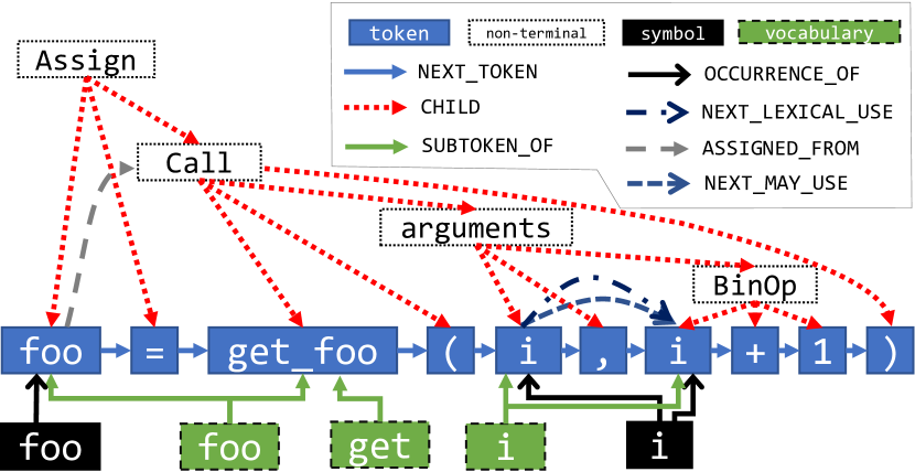
Figure 3. Sample graph for foo=get_foo(i, i+1) showing different node categories and edge labels.

Our graphs are extracted per-file, excluding all comments, using the typed_ast and symtable Python packages by performing a dataflow analysis. Fig. 3 illustrates such a graph. Our graph consists of four categories of nodes:

• token nodes represent the raw lexemes in the program.

• non-terminal nodes of the syntax tree.

• vocabulary nodes that represents a subtoken (Cvitkovic et al., 2019), i.e. a word-like element which is retrieved by splitting an identifier into parts on camelCase or pascal_case.

• symbol nodes that represent a unique symbol in the symbol table, such as a variable or function parameter.

For a symbol $s$, we set its type embeddings to $\boldsymbol{r}_{s}=\boldsymbol{h}^{t=T}_{n_{s}}$ where $n_{s}$ is $s$’s symbol node. Symbol nodes are similar to Gilmer et al. (2017)’s “supernode”. For functions, we introduce a symbol node for each parameter and a separate symbol node for their return. We combine these to retrieve its signature.

We use edges to codify relationships among nodes, which the GNN uses in the output representations. As is usual in deep learning, we do not know the fine-grained impact of different edges, but we do know and report (Sec. 6.2) the impact of their ablation on the overall performance. Table 1 details our edge labels. Though some labels appear irrelevant from the perspective of traditional program analysis, previous work has demonstrated that they are useful in capturing code patterns indicative of code properties. In Table 1, we cite the work that inspired us to use each edge label. For example, NEXT_TOKEN is redundant in program analysis (and would be discarded after parsing) but is quite predictive (Allamanis et al., 2018b; Hellendoorn et al., 2018). Particularly important to our approach are the OCCURRENCE_OF edges. For example, a variable-bound token node x will be connected to its variable symbol node, or a member access AST node self.y will be connected to the relevant symbol node. This edge label allows different uses of the same symbol to exchange information in the GNN.

The AST encodes syntactic information that is traditionally used in type inference (e.g. assignment and operators) so the GNN learns about these relationships. Function invocations are not treated specially (i.e. linked to their definitions), since, in a partially annotated codebase, statically resolving the receiver object and thence the function is often too imprecise. Instead, the GNN incorporates the name of the invoked function and the names of all its keyword arguments, which in Python take the form of foo(arg_name=value).

Finally, SUBTOKEN_OF connects all identifiers that contain a subtoken to a unique vocabulary node representing the subtoken. As Cvitkovic et al. (2019) found, this category of edges significantly improves a model’s performance on the task of detecting variable misuses and suggesting variable names. It represents textual similarities among names of variables and functions, even if these names are previously unseen. For example, a variable name numNodes and a function name getNodes, share the same subtoken nodes. By adding this edge, the GNN learns about the textual similarity of the different elements of the program, capturing patterns that depend on the words used by the developer.

6. Quantitative Evaluation

predicts types where traditional type inference cannot. However, some of its predictions may be incorrect, hampering ’ utility. In this section, we quantitatively evaluate the types predicts against two forms of ground-truth: (a) how often the predictions match existing type annotations (Sec. 6.1, Sec. 6.2) and (b) how often the predictions pass optional type checking (Sec. 6.3).

Data

We select real-world Python projects that care about types; these are the projects likely to adopt . As a proxy, we use regular expressions to collect 600 Python repositories from GitHub that contain at least one type annotation. We then clone those repositories and run pytype to augment our corpus with type annotations that can be inferred from a static analysis tool. To allow pytype to infer types from imported libraries, we add to the Python environment the top 175 most downloaded libraries.

Then, we run the deduplication tool of Allamanis (2019). Similar to the observations of Lopes et al. (2017), we find a substantial number of (near) code duplicates in our corpus — more than 133k files. We remove all these duplicate files keeping only one exemplar per cluster of duplicates. As discussed in Allamanis (2019), failing to remove those files would significantly bias our results. We provide a Docker container that replicates corpus construction and a list of the cloned projects (and SHAs) at https://github.com/typilus/typilus.

The collected dataset is made of 118 440 files with a total 5 997 459 symbols of which 252 470 have a non-Any non-None type annotation. The annotated types are quite diverse, and follow a heavy-tailed distribution. There are about 24.7k distinct non-Any types, but the top 10 types are about half of the dataset. Unsurprisingly, the most common types are str, bool and int appearing 86k times in total. Additionally, we find only 158 types with more than 100 type annotations, where each one of the rest 25k types are used within an annotation less than 100 times per type, but still amount to 32% of the dataset. This skew in how type annotations are used illustrates the importance of correctly predicting annotations not just for the most frequent types but for the long tail of rarer types. The long-tail of types, consist of user-defined types and generic types with different combinations of type arguments. Finally, we split our data into train-validation-test set in 70-10-20 proportions.

6.1. Quantitative Evaluation

Next, we look at the ability of our model to predict ground-truth types. To achieve this, we take existing code, erase all type annotations and aim to retrieve the original annotations.

Measures

Measuring the ability of a probabilistic system that predicts types is a relatively new domain. For a type prediction $\tau_{p}$ and the ground truth type $\tau_{g}$, we propose three criteria and measure the performance of a type predicting system by computing the ratio of predictions, over all predictions, that satisfy each criterion:

Exact Match:

$\tau_{p}$ and $\tau_{g}$ match exactly.

Match up to Parametric Type:

Exact match when ignoring all type parameters (outermost []).

Type Neutral:

$\tau_{p}$ and $\tau_{g}$ are neutral, or interchangeable, under optional typing.

In Sec. 6.1 and Sec. 6.2, we approximate type neutrality. We preprocess all types seen in the corpus, rewriting components of a parametric type whose nested level is greater than 2 to Any. For example, we rewrite List[List[List[int]]] to List[List[Any]]. We then build a type hierarchy for the preprocessed types. Assuming universal covariance, this type hierarchy is a lattice ordered by subtyping $:<$. We heuristically define a prediction $\tau_{p}$ to be neutral with the ground-truth $\tau_{g}$ if $\tau_{g}:<\tau_{p}\wedge\tau_{p}\neq\top$ in the hierarchy. This approximation is unsound, but fast and scalable. Despite being unsound, the supertype still conveys useful information, facilitating program comprehension and searching for $\tau_{g}$. In Sec. 6.3, we assess type neutrality by running an optional type checker. We replace $\tau_{g}$ in a partially annotated program $P$ with $\tau_{p}$, creating a new program $P^{\prime}$, and optionally type check $P^{\prime}$ to observe whether the replacement triggers a type error. Note that an optional type checker’s assessment of type neutrality may change as $P$ becomes more fully annotated.

Baselines

The first set of baselines — prefixed with “Seq” — are based on DeepTyper (Hellendoorn et al., 2018). Exactly as in DeepTyper, we use 2-layer biGRUs (Bahdanau et al., 2015) and a consistency module in between layers. The consistency module computes a single representation for each variable by averaging the vector representations of the tokens that are bound to the same variable. Our models are identical to DeepTyper with the following exceptions (a) we use subtoken-based embeddings which tend to help generalisation (b) we add the consistency module to the output biGRU layer, retrieving a single representation per variable. Using this method, we compute the type embedding of each variable.

The second set of baselines (denoted as *Path) are based on code2seq (Alon et al., 2010). We adapt code2seq from its original task of predicting sequences to predicting a single vector by using a self-weighted average of the path encodings similar to Gilmer et al. (2017). For each symbol, we sample paths that involve that tokens of that symbol and other leaf identifier nodes. We use the hyperparameters of Alon et al. (2010).

We test three variations for the Seq-based, Path-based, and graph-based models. The models suffixed with Class use the classification-based loss (Eq. 1), those suffixed with Space use similarity learning and produce a type space (Eq. 3). Finally, models suffixed with use the full loss (Eq. 4). The *Space and *models differ only in the training objective, but are otherwise identical.

Results

	Loss	% Exact Match				% Match up to Parametric Type			% Type
		All	Common	Rare		All	Common	Rare	Neutral
Seq2Class	Eq. 1	39.6	63.8	4.6		41.2	64.6	7.6	30.4
Seq2Space	Eq. 3	47.4	62.2	24.5		51.8	63.7	32.2	48.9
Seq-	Eq. 4	52.4	71.7	24.9		59.7	74.2	39.3	53.9
Path2Class	Eq. 1	37.5	60.5	5.2		39.0	61.1	7.9	34.0
Path2Space	Eq. 3	42.3	61.9	14.5		47.4	63.6	24.8	43.7
Path-	Eq. 4	43.2	63.8	13.8		49.2	65.8	25.7	44.7
Graph2Class	Eq. 1	46.1	74.5	5.9		48.8	75.4	11.2	46.9
Graph2Space	Eq. 3	50.5	69.7	23.1		58.4	72.5	38.4	51.9
	Eq. 4	54.6	77.2	22.5		64.1	80.3	41.2	56.3

Table 2. Quantitative evaluation of models measuring their ability to predict ground truth type annotations. Breakdown for common (seen $\geq 100$ times) and rare types (seen $<100$ times). Results averaged over two randomly initialised trainings.

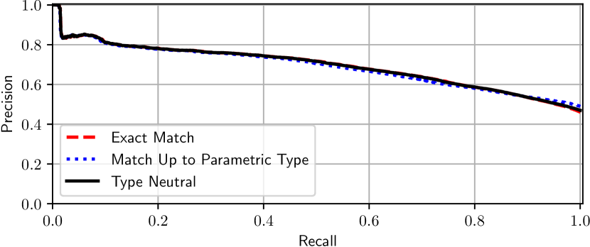
(a) Graph2Class

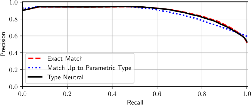
(b) Graph2Space

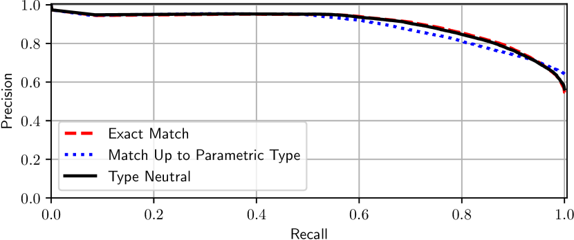
(c)

Figure 4. Precision-recall Curves. When filtering by confidence, makes precise predictions; compared to the baselines, 95% of the predictions are type neutral, when predicts a type to 60% of all symbols (i.e. 60% recall).

Table 2 shows the results of the various methods and variations. First, it shows that the graph-based models outperform the sequence-based and path-based models on most metrics, but not by a wide margin. This suggests that graphs capture the structural constraints of the code somewhat better than sequence models. When we break down the results into the types that are often seen in our test set (we arbitrarily define types seen fewer than 100 times to be rare), we see that the meta-learning learning methods are significantly better at predicting the rare types and perform only slightly worse than classification-based models on the more common types. Combining meta-learning and classification (loss in Eq. 4) yields the best results. The Path-based methods (Alon et al., 2010) perform slightly worse to the sequence-based methods. We believe that this is because sequence models treat the problem as structured prediction (predicting the type of multiple symbols simultaneously), whereas path-based models make independent predictions.

Fig. 5 breaks down the performance of by the number of times each type is seen in an annotation. Although performance drops for rare annotations the top prediction is often valid. Since a type checker can eliminate false positives, the valid predictions will improve ’s performance.

The precision-recall curve of in Fig. 4 shows that it achieves high type neutrality for high-confidence predictions compared to the baselines. This suggests that, if we threshold on the prediction’s confidence, we can vary the precision-recall trade-off. In particular, the curve shows that achieves a type neutrality of about 95% when predicting types for 70% of the symbols, implying that this method works well enough for eventual integration into a useful tool. As we discuss in Sec. 6.3, we further eliminate false positives by filtering the suggestions through a type checker, which removes “obviously incorrect” predictions. Table 3 shows the breakdown of the performance of over different kinds of symbols. seems to perform worse on variables compared to other symbols on exact match, but not on match up to the parametric type. We believe that this is because in our data variable annotations are more likely to involve generics compared to parameter or return annotations.

	Var	Func
		Para	Ret
% Exact Match	43.5	53.8	56.9
% Match up to Parametric Type	61.8	57.9	69.5
% Type Neutral	45.5	55.1	58.9
Proportion of testset	9.4%	41.5%	49.1%

Table 3. ’s performance by the kind of symbol.

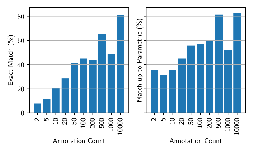
Figure 5. ’s performance bucketed by the number of annotations of a given type in our dataset.

Relating Results to JavaScript

The results presented here are numerically worse than those for JavaScript corpora presented in JSNice (Raychev et al., 2015) and DeepTyper (Hellendoorn et al., 2018). We posit three reasons for this difference. First, ’s Python dataset and the previous work’s JavaScript datasets differ significantly in the targeted application domains. Second, code duplicated, or shared, across the training and test corpora of the previous work may have affected the reported results (Allamanis, 2019). Third, the dynamic type systems of Python and JavaScript are fundamentally different. Python features a type system that supports many type constructors and enforces strict dynamic type checking. This has encouraged developers to define type hierarchies that exploit the error checking it offers. In contrast, JavaScript’s dynamic type system is less expressive and more permissive. The detailed, and sparse, type hierarchies that Python programs tend to have makes predicting type annotations harder in Python than in JavaScript.

Computational Speed

The GNN-based models are significantly faster compared to RNN-based models. On a Nvidia K80 GPU, a single training epoch takes 86sec for the GNN model, whereas it takes 5 255sec for the biRNN model. Similarly, during inference the GNN model is about 29 times faster taking only 7.3sec per epoch (i.e. less than 1ms per graph on average). This is due to the fact that the biRNN-based models cannot parallelise the computation across the length of the sequence and thus computation time is proportional to the length of the sequence, whereas GNNs parallelise the computation but at the cost of using information that is only a few hops away in the graph. However, since the graph (by construction) records long-range information explicitly (e.g. data flow) this does not impact the quality of predictions.

Transformers

An alternative to RNN-based models are transformers (Vaswani et al., 2017), which have recently shown exceptional performance in natural language processing. Although transformers can be parallelised efficiently, their memory requirements are quadratic to the sequence length. This is prohibitive for even moderate Python files. We test small transformers (replacing the biGRU of our DeepTyper) and remove sequences with more than 5k tokens, using a mini-batch size of 2. The results did not improve on DeepTyper. This may be because transformers often require substantially larger quantities of data to outperform other models.

6.2. Ablation Analysis

Now, we test ’s performance when varying different elements of its architecture. Our goal is not to be exhaustive, but to illustrate how different aspects affect type prediction. Table 4 shows the results of the ablation study, where we remove some edge labels from the graph at a time and re-train our neural network from scratch. The results illustrate the (un)importance of each aspect of the graph construction, which Sec. 5 detailed. First, if we simply use the names of the symbol nodes the performance drops significantly and the model achieves an exact match of 37.6%. Nevertheless, this is a significant percentage and attests to the importance of the noisy, but useful, information that identifiers contain. Removing the syntactic edges, NEXT_TOKEN and CHILD, also reduces the model’s performance, showing that our model can find patterns within these edges. Interestingly, if we just remove NEXT_TOKEN edges, we still see a performance reduction, indicating that tokens — traditionally discarded in formal analyses, since they are redundant — can be exploited to facilitate type prediction. Finally, the data-flow related edges, NEXT_LEXICAL_USE and NEXT_MAY_USE, have negligible impact on the overall performance. The reason is that for type prediction, the order of a symbol’s different uses does not matter. Therefore, representing these uses in a sequence (NEXT_LEXICAL_USE) or a tree (NEXT_MAY_USE) offers no additional benefits. Simply put, OCCURRENCE_OF subsumes NEXT_*USE in our problem setting.

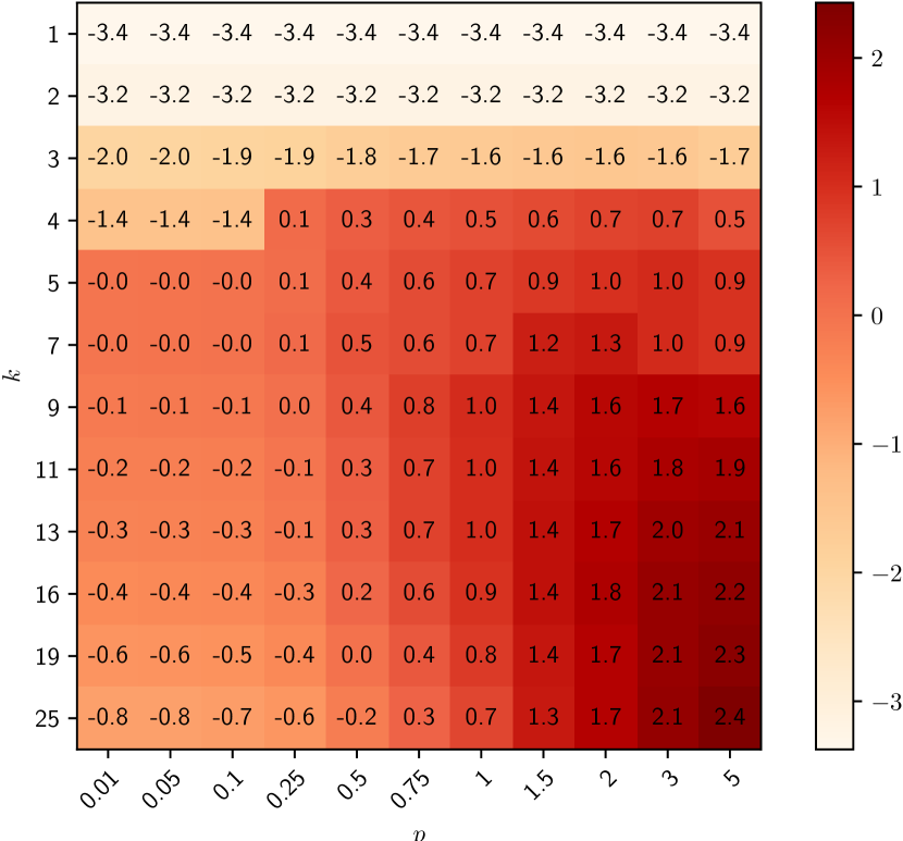
Figure 6. Absolute difference in match up to parametric type for w.r.t. median for various $k$ and $p$ in eq. 5.

Table 4 also shows how the performance of varies with different token representations for the initial node states of the GNN. We test two variations: Token-level representations, where each lexeme gets a single embedding as in Hellendoorn et al. (2018), and character-level representations that use a 1D convolutional neural network (Kim et al., 2016) to compute a node representation from its characters. The results suggest that the initial representation does not have a big difference, with ’s subtoken-level models having a small advantage, whereas the character-level CNN models performing the worst, but with a small difference.

Finally, Fig. 6 shows ’s performance when varying $k$ and $p$ of Eq. 5. The results suggest that larger values for $k$ give better results and a larger $p$ also helps, suggesting that looking at a wider neighbourhood in the type map but accounting for distance can yield more accurate results.

Ablation	Exact Match	Type Neutral
Only Names (No GNN)	38.8%	40.4%
No Syntactic Edges	53.7%	55.6%
No NEXT_TOKEN	54.7%	56.3%
No CHILD	48.4%	50.2%
No NEXT_*USE	54.7%	56.4%
Full Model – Tokens	53.7%	55.4%
Full Model – Character	53.4%	55.0%
Full Model – Subtokens	54.6%	56.3%

Table 4. Ablations of when removing edges from the graph or varying the initial node representation.

6.3. Correctness Modulo Type Checker

So far, we treated existing type annotations — those manually added by the developers or those inferred by pytype — as the ground-truth. However, as we discuss in Sec. 7, some annotations can be wrong, e.g. because developers may not be invoking a type checker and many symbols are not annotated. To thoroughly evaluate , we now switch to a different ground truth: optional type checkers. Though optional type checkers reason over only a partial context with respect to a fully-typed program and are generally unsound, their best-effort is reasonably effective in practice (Gao et al., 2017). Thus, we take their output as the ground-truth here.

Specifically, we test one type prediction at a time and pick the top prediction for each symbol. For each prediction $\tau$ for a symbol $s$ in an annotated program $P$, we add $\tau$ to $P$ if $s$ is not annotated, or replace the existing annotation for $s$ with $\tau$, retaining all other annotations in $P$. Then, we run the optional type checker and check if $\tau$ causes a type error. We repeat this process for all the top predictions and aggregate the results. This experiment reflects the ultimate goal of : helping developers gradually move an unannotated or partially annotated program to a fully annotated program by adding a type prediction at a time.

We consider two optional type checkers: mypy and pytype. In 2012, mypy introduced optional typing for Python and strongly inspires Python’s annotation syntax. Among other tools, pytype stands out because it employs more powerful type inference and more closely reflects Python’s semantics, i.e. it is less strict in type checking than a traditional type checker, like mypy. Both type checkers are popular and actively maintained, but differ in design mindset, so we include both to cover different philosophies on optional typing.

To determine how often ’s type predictions are correct, we first discard any programs which fail to type check before using , since they will also fail even when ’s type predictions are correct. Since mypy and pytype also perform other static analyses, such as linting and scope analysis, we need to isolate the type-related errors. To achieve this, we comb through all error classes of mypy and pytype and, based on their description and from first principles, decide which errors relate to types. We then use these type-related error classes to filter the programs in our corpus. This filter is imperfect: some error classes, like “[misc]” in mypy, mix type errors with other errors. To resolve this, we sample the filtered programs and manually determine whether the sampled programs have type errors. This process removes 229 programs for mypy and 10 programs for pytype that escaped the automated filtering based on error classes. We provide more information at https://github.com/typilus/typilus. After preprocessing the corpus, we run mypy and pytype on the remaining programs, testing one prediction at a time. We skip type predictions which are Any, or on which mypy or pytype crashes or spends more than 20 seconds. In total, we assess 350,374 type predictions using mypy and 85,732 using pytype.

Annotation			mypy			pytype
Original	Predicted		Prop.	Acc.		Prop.	Acc.
$\epsilon$	$\tau$		95%	89%		94%	83%
$\tau$	$\tau^{\prime}$		3%	85%		3%	63%
$\tau$	$\tau$		2%	100%		3%	100%
Overall			100%	89%		100%	83%

Table 5. Type checking accuracy of modulo mypy and pytype. A prediction is incorrect if it causes a type error. Mypy and pytype experience timeouts on different programs, hence the discrepancy between the proportion of each case.

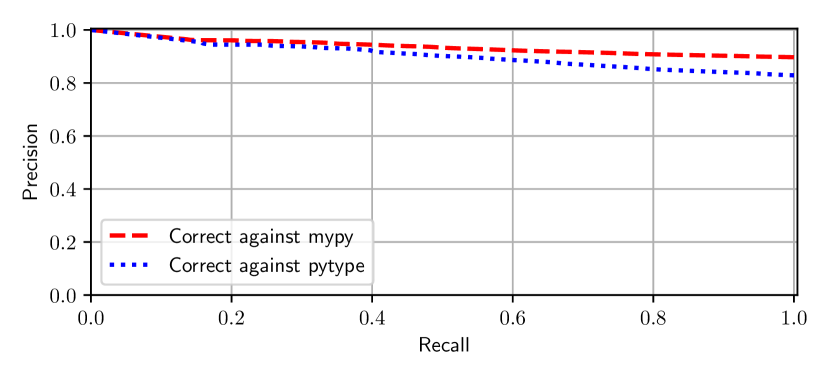
Figure 7. Precision-recall curve for the type checking experiment. We deem unable to suggest a type if the probability of a type prediction is below a threshold.

Table 5 presents the results of applying mypy and pytype to the top type predictions. In general, 89% and 83% of ’s predictions do not cause a type error in mypy and pytype, respectively. This demonstrates that the type predictions are commonly correct with respect to optional typing. We then group the predictions into three categories: $\epsilon\rightarrow\tau$ where suggests a type to a previously unannotated symbol, $\tau\rightarrow\tau^{\prime}$ where it suggests a type that is different from the original annotation, and $\tau\rightarrow\tau$ where the suggested type is identical with the original annotation. As the $\epsilon\rightarrow\tau$ row illustrates, most of the symbols, whose types is able to predict, are untyped even after pytype’s type inference. This indicates that has a wide application domain.

For mypy, 3% of ’s predictions differ from the original annotations. Though different, some of these predictions might actually be correct (Sec. 7). Further analysis reveals that 33% of these predictions are a supertype of the original one (less precise but interchangeable) and 2% are more specific (and potentially but not certainly incorrect). Mypy produces a type error for 22% of them, which shows that optional type checkers can effectively improve the quality ’s suggestion, by filtering false positives. The $\tau\rightarrow\tau$ case is a sanity check: the input programs do not have type errors, by construction of this experiment, so when predicts the same annotations, they pass type checking.

Finally, Fig. 7 investigates ’ precision and recall. By varying the confidence threshold on the predictions, we can trade precision for recall. maintains a good trade-off between precision and recall. For example, when it predicts a type for 80% of all symbols, 90% of the predictions are correct with respect to mypy.

7. Qualitative Evaluation

To better understand the performance of and the expressivity of the types it can infer, we manually analyse its predictions, before a type checker filters them. Our goal is not to be exhaustive but to convey cases that indicate opportunities for future research.

We begin by exploring how complex a type expression can reliably infer. By complex, we mean a deeply nested parametric type such as Set[Tuple[bool, Tuple[UDT, ...]]], where UDT denotes a user-defined type. In principle, can learn to predict these types. However, such types are extremely rare in our dataset: about 30% of our annotations are parametric and, of them, 80% have depth one and 19% have depth two, with more deeply nested types mostly appearing once. For our evaluation, we built the type map over the training and the validation sets. Since these complex types appear once (and only in our test set), they do not appear in the type map and cannot predict them. We believe that deeply nested parametric types are so rare because developers prefer to define and annotate UDTs rather than deeply nested types which are hard-to-understand. Unfortunately, finds UDTs hard to predict. Improved performance on the task will require machine learning methods that better understand the structure of UDTs and the semantics of their names.

We now look at the most confident errors, i.e. cases where confidently predicts a non-type neutral type. commonly confuses variables with collections whose elements have the same type as the variables, confusing T and Optional[T], for various concrete T, and predicts the wrong type. Similarly, when the ground truth type is a Union, often predicts a subset of the types in the union. This suggests that the type space is not learning to represent union types. For example, in rembo10/headphones, predicts Optional[int] where the ground truth is Optional[Union[float, int, str]]. Adding intraprocedural relationships to , especially among different code files, may help resolve such issues.

We also identified a few cases where the human type annotation is wrong. For example, in PyTorch/fairseq, a sequence-to-sequence modelling toolkit that attracts more than 7.3k stars on GitHub, we found three parameters representing tensor dimensions annotated as float. , having seen similar code and similarly named variables, predicts with 99.8% confidence that these parameters should be annotated as int. We submitted two pull requests covering such cases: one to PyTorch/fairseq and one to allenai/allennlp, a natural language processing library with more than 8.2k stars. Both have been merged. Why did the type checker fail to catch these errors? The problem lies with the nature of optional typing. It can only reason locally about type correctness; it only reports an error if it finds a local type inconsistency. When a function invokes an unannotated API, an optional type checker can disprove very few type assignments involving that call. This is an important use-case of , where, due to the sparsely annotated nature of Python code, incorrect annotations can go undetected by type checkers.

In some cases, predicts a correct, but more specific type, than the original type annotation or the one inferred by pytype. For example, in an Ansible function, pytype inferred dict, whereas predicted the more precise Dict[str, Any]. We believe that this problem arises due to pytype’s design, such as preferring conservative approximations, which allow it to be a practical type inference engine.

A third source of disagreement with the ground truth is confusing str and bytes. These two types are conceptually related: bytes are raw while str is “cooked” Unicode. Indeed, one can always encode a str into its bytes and decode it back to a str, given some encoding such as ASCII or UTF-8. Python developers also commonly confuse them (Overflow, 2011), so it is not surprising that does too. We believe that this confusion is due to the fact that variables and parameters of the two types have a very similar interface and they usually share names. Resolving this will require a wider understanding how the underlying object is used, perhaps via an approximate intraprocedural analysis.

Finally, confuses some user-defined types. Given the sparsity of these types, this is unsurprising. Often, the confusion is in conceptually related types. For example, in awslabs/sockeye, a variable annotated with mx.nd.NDArray is predicted to be torch.Tensor. Interestingly, these two types represent tensors but in different machine learning frameworks (MxNet and PyTorch).

8. Related Work

Recently, researchers have been exploring the application of machine learning to code (Allamanis et al., 2018a). This stream of work focuses on capturing (fuzzy) patterns in code to perform tasks that would not be possible with using only formal methods. Code completion (Raychev et al., 2014; Hindle et al., 2012; Hellendoorn and Devanbu, 2017; Karampatsis and Sutton, 2019) is one of the most widely explored topics. Machine learning models of code are also used to predict names of variables and functions (Allamanis et al., 2014, 2015a; Alon et al., 2019, 2010; Bavishi et al., 2018), with applications to deobfuscation (Raychev et al., 2015; Vasilescu et al., 2017) and decompilation (He et al., 2018; David et al., 2019; Lacomis et al., 2019). Significant effort has been made towards automatically generating documentation from code or vice versa (Iyer et al., 2016; Barone and Sennrich, 2017; Alon et al., 2010; Fernandes et al., 2019). These works demonstrate that machine learning can effectively capture patterns in code.

Program Analysis and Machine Learning

Within the broader area of program analysis, machine learning has been utilised in a variety of settings. Recent work has focused on detecting specific kinds of bugs, such as variable misuses and argument swappings (Allamanis et al., 2018b; Cvitkovic et al., 2019; Pradel and Sen, 2017; Vasic et al., 2019; Rice et al., 2017) showing that “soft” patterns contain valuable information that can catch many real-life bugs that would not be otherwise easy to catch with formal program analysis. Work also exists in a variety of program analysis domains. Si et al. (2018) learn to predict loop invariants, Mangal et al. (2015) and Heo et al. (2019) use machine learning methods to filter false positives from program analyses by learning from user feedback. Chibotaru et al. (2019) use weakly supervised learning to learn taint specifications and DeFreez et al. (2018) mine API call sequence specifications.

Code Representation in Machine Learning

Representing code for consumption in machine learning is a central research problem. Initial work viewed code as a sequence of tokens (Hindle et al., 2012; Hellendoorn and Devanbu, 2017). The simplicity of this representation has allowed great progress, but it misses the opportunity to learn from code’s known and formal structure. Other work based their representation on ASTs (Maddison and Tarlow, 2014; Bielik et al., 2016; Allamanis et al., 2015b; Alon et al., 2019, 2010) — a crucial step towards exploitation of code’s structure. Finally, graphs, which employs, encode a variety of complex relationships among the elements of code. Examples of include the early works of Kremenek et al. (2007) and Raychev et al. (2015) and variations of GNNs (Allamanis et al., 2018b; Cvitkovic et al., 2019; Heo et al., 2019).

Optional Typing

At the core of optional typing (Bracha, 2004) lie optional type annotations and pluggable type checking, combining static and dynamic typing, but without providing soundness guarantees. Therefore, it is often called “unsound gradual typing” (Takikawa et al., 2016; Muehlboeck and Tate, 2017). Optional typing has not been formalised and its realisation varies across languages and type checkers. For example, TypeScript checks and then erases type annotations, whereas Python’s type annotations simply decorate the code, and are used by external type checkers.

9. Conclusion

We presented a machine learning method for predicting types in dynamically typed languages with optional annotations and realised it for Python. Type inference for many dynamic languages, like Python, must often resort to the Any type. Machine learning methods, like the one presented here, that learn from the rich patterns within the code, including identifiers and coding idioms, can provide an approximate, high-precision and useful alternative.

- (1)
- Allamanis (2019) Miltiadis Allamanis. 2019. The Adverse Effects of Code Duplication in Machine Learning Models of Code. In SPLASH Onward!
- Allamanis et al. (2014) Miltiadis Allamanis, Earl T Barr, Christian Bird, and Charles Sutton. 2014. Learning Natural Coding Conventions. In Proceedings of the International Symposium on Foundations of Software Engineering (FSE).
- Allamanis et al. (2015a) Miltiadis Allamanis, Earl T Barr, Christian Bird, and Charles Sutton. 2015a. Suggesting accurate method and class names. In Proceedings of the Joint Meeting of the European Software Engineering Conference and the Symposium on the Foundations of Software Engineering (ESEC/FSE).
- Allamanis et al. (2018a) Miltiadis Allamanis, Earl T Barr, Premkumar Devanbu, and Charles Sutton. 2018a. A survey of machine learning for big code and naturalness. ACM Computing Surveys (CSUR) 51, 4 (2018), 81.
- Allamanis et al. (2018b) Miltiadis Allamanis, Marc Brockschmidt, and Mahmoud Khademi. 2018b. Learning to Represent Programs with Graphs. In Proceedings of the International Conference on Learning Representations (ICLR).
- Allamanis and Sutton (2013) Miltiadis Allamanis and Charles Sutton. 2013. Mining source code repositories at massive scale using language modeling. In Proceedings of the Working Conference on Mining Software Repositories (MSR). IEEE Press, 207–216.
- Allamanis et al. (2015b) Miltiadis Allamanis, Daniel Tarlow, Andrew Gordon, and Yi Wei. 2015b. Bimodal modelling of source code and natural language. In Proceedings of the International Conference on Machine Learning (ICML).
- Alon et al. (2010) Uri Alon, Omer Levy, and Eran Yahav. 2010. code2seq: Generating Sequences from Structured Representations of Code. In Proceedings of the International Conference on Learning Representations (ICLR).
- Alon et al. (2019) Uri Alon, Meital Zilberstein, Omer Levy, and Eran Yahav. 2019. code2vec: Learning distributed representations of code. Proceedings of the ACM on Programming Languages 3, POPL (2019), 40.
- Bahdanau et al. (2015) Dzmitry Bahdanau, Kyunghyun Cho, and Yoshua Bengio. 2015. Neural machine translation by jointly learning to align and translate. In Proceedings of the International Conference on Learning Representations (ICLR).
- Barone and Sennrich (2017) Antonio Valerio Miceli Barone and Rico Sennrich. 2017. A Parallel Corpus of Python Functions and Documentation Strings for Automated Code Documentation and Code Generation. In Proceedings of the Eighth International Joint Conference on Natural Language Processing (Volume 2: Short Papers), Vol. 2. 314–319.
- Bavishi et al. (2018) Rohan Bavishi, Michael Pradel, and Koushik Sen. 2018. Context2Name: A deep learning-based approach to infer natural variable names from usage contexts. arXiv preprint arXiv:1809.05193 (2018).
- Bielik et al. (2016) Pavol Bielik, Veselin Raychev, and Martin Vechev. 2016. PHOG: Probabilistic Model for Code. In Proceedings of the International Conference on Machine Learning (ICML). 2933–2942.
- Bracha (2004) Gilad Bracha. 2004. Pluggable type systems. In OOPSLA workshop on revival of dynamic languages, Vol. 4.
- Brockschmidt et al. (2019) Marc Brockschmidt, Miltiadis Allamanis, Alexander L Gaunt, and Oleksandr Polozov. 2019. Generative code modeling with graphs. In International Conference in Learning Representations.
- Cheng et al. (2016) De Cheng, Yihong Gong, Sanping Zhou, Jinjun Wang, and Nanning Zheng. 2016. Person re-identification by multi-channel parts-based CNN with improved triplet loss function. In Proceedings of the IEEE conference on computer vision and pattern recognition. 1335–1344.
- Chibotaru et al. (2019) Victor Chibotaru, Benjamin Bichsel, Veselin Raychev, and Martin Vechev. 2019. Scalable taint specification inference with big code. In Proceedings of the 40th ACM SIGPLAN Conference on Programming Language Design and Implementation. ACM, 760–774.
- Cho et al. (2014) Kyunghyun Cho, Bart van Merriënboer, Dzmitry Bahdanau, and Yoshua Bengio. 2014. On the Properties of Neural Machine Translation: Encoder–Decoder Approaches. Syntax, Semantics and Structure in Statistical Translation (2014).
- Chopra et al. (2005) Sumit Chopra, Raia Hadsell, and Yann LeCun. 2005. Learning a similarity metric discriminatively, with application to face verification. In CVPR.
- Cvitkovic et al. (2019) Milan Cvitkovic, Badal Singh, and Anima Anandkumar. 2019. Open Vocabulary Learning on Source Code with a Graph-Structured Cache. In Proceedings of the International Conference on Machine Learning (ICML).
- Dash et al. (2018) Santanu Kumar Dash, Miltiadis Allamanis, and Earl T Barr. 2018. RefiNym: using names to refine types. In Proceedings of the 2018 26th ACM Joint Meeting on European Software Engineering Conference and Symposium on the Foundations of Software Engineering. ACM, 107–117.
- David et al. (2019) Yaniv David, Uri Alon, and Eran Yahav. 2019. Neural Reverse Engineering of Stripped Binaries. arXiv preprint arXiv:1902.09122 (2019).
- DeFreez et al. (2018) Daniel DeFreez, Aditya V Thakur, and Cindy Rubio-González. 2018. Path-based function embedding and its application to specification mining. arXiv preprint arXiv:1802.07779 (2018).
- Fernandes et al. (2019) Patrick Fernandes, Miltiadis Allamanis, and Marc Brockschmidt. 2019. Structured neural summarization.
- Foundation (2020) Python Software Foundation. 2020. typing – Support for type hints. https://docs.python.org/3/library/typing.html. Visited March 2020.
- Gao et al. (2017) Zheng Gao, Christian Bird, and Earl T Barr. 2017. To type or not to type: quantifying detectable bugs in JavaScript. In Proceedings of the International Conference on Software Engineering (ICSE).
- Gilmer et al. (2017) Justin Gilmer, Samuel S Schoenholz, Patrick F Riley, Oriol Vinyals, and George E Dahl. 2017. Neural message passing for quantum chemistry. In Proceedings of the 34th International Conference on Machine Learning-Volume 70. JMLR. org, 1263–1272.
- Goodfellow et al. (2016) Ian Goodfellow, Yoshua Bengio, and Aaron Courville. 2016. Deep Learning. MIT Press. www.deeplearningbook.org.
- Hadsell et al. (2006) Raia Hadsell, Sumit Chopra, and Yann LeCun. 2006. Dimensionality reduction by learning an invariant mapping. In 2006 IEEE Computer Society Conference on Computer Vision and Pattern Recognition (CVPR’06), Vol. 2. IEEE, 1735–1742.
- He et al. (2018) Jingxuan He, Pesho Ivanov, Petar Tsankov, Veselin Raychev, and Martin Vechev. 2018. Debin: Predicting debug information in stripped binaries. In Proceedings of the 2018 ACM SIGSAC Conference on Computer and Communications Security. ACM, 1667–1680.
- Hellendoorn et al. (2018) Vincent J Hellendoorn, Christian Bird, Earl T Barr, and Miltiadis Allamanis. 2018. Deep learning type inference. In Proceedings of the 2018 26th ACM Joint Meeting on European Software Engineering Conference and Symposium on the Foundations of Software Engineering. ACM, 152–162.
- Hellendoorn and Devanbu (2017) Vincent J Hellendoorn and Premkumar Devanbu. 2017. Are deep neural networks the best choice for modeling source code?. In Proceedings of the 2017 11th Joint Meeting on Foundations of Software Engineering. ACM, 763–773.
- Heo et al. (2019) Kihong Heo, Mukund Raghothaman, Xujie Si, and Mayur Naik. 2019. Continuously reasoning about programs using differential Bayesian inference. In Proceedings of the 40th ACM SIGPLAN Conference on Programming Language Design and Implementation. ACM, 561–575.
- Hindle et al. (2012) Abram Hindle, Earl T Barr, Zhendong Su, Mark Gabel, and Premkumar Devanbu. 2012. On the naturalness of software. In Software Engineering (ICSE), 2012 34th International Conference on. IEEE, 837–847.
- Iyer et al. (2016) Srinivasan Iyer, Ioannis Konstas, Alvin Cheung, and Luke Zettlemoyer. 2016. Summarizing source code using a neural attention model. In Proceedings of the 54th Annual Meeting of the Association for Computational Linguistics (Volume 1: Long Papers), Vol. 1. 2073–2083.
- Karampatsis and Sutton (2019) Rafael-Michael Karampatsis and Charles Sutton. 2019. Maybe Deep Neural Networks are the Best Choice for Modeling Source Code. arXiv preprint arXiv:1903.05734 (2019).
- Kate et al. (2018) Sayali Kate, John-Paul Ore, Xiangyu Zhang, Sebastian Elbaum, and Zhaogui Xu. 2018. Phys: probabilistic physical unit assignment and inconsistency detection. In Proceedings of the 2018 26th ACM Joint Meeting on European Software Engineering Conference and Symposium on the Foundations of Software Engineering. ACM, 563–573.
- Kim et al. (2016) Yoon Kim, Yacine Jernite, David Sontag, and Alexander M Rush. 2016. Character-aware neural language models. In Thirtieth AAAI Conference on Artificial Intelligence.
- Kipf and Welling (2016) Thomas N Kipf and Max Welling. 2016. Semi-supervised classification with graph convolutional networks. arXiv preprint arXiv:1609.02907 (2016).
- Kremenek et al. (2007) Ted Kremenek, Andrew Y Ng, and Dawson R Engler. 2007. A Factor Graph Model for Software Bug Finding. In Proceedings of the International Joint Conference on Artifical intelligence (IJCAI).
- Lacomis et al. (2019) Jeremy Lacomis, Pengcheng Yin, Edward J Schwartz, Miltiadis Allamanis, Claire Le Goues, Graham Neubig, and Bogdan Vasilescu. 2019. DIRE: A Neural Approach to Decompiled Identifier Naming. In Proceedings of the International Conference on Automated Software Engineering (ASE).
- Li et al. (2016) Yujia Li, Daniel Tarlow, Marc Brockschmidt, and Richard Zemel. 2016. Gated Graph Sequence Neural Networks. Proceedings of the International Conference on Learning Representations (ICLR) (2016).
- Livshits et al. (2015) Benjamin Livshits, Manu Sridharan, Yannis Smaragdakis, Ondřej Lhoták, J Nelson Amaral, Bor-Yuh Evan Chang, Samuel Z Guyer, Uday P Khedker, Anders Møller, and Dimitrios Vardoulakis. 2015. In defense of soundiness: a manifesto. Commun. ACM 58, 2 (2015), 44–46.
- Lopes et al. (2017) Cristina V Lopes, Petr Maj, Pedro Martins, Vaibhav Saini, Di Yang, Jakub Zitny, Hitesh Sajnani, and Jan Vitek. 2017. DéjàVu: a map of code duplicates on GitHub. Proceedings of the ACM on Programming Languages 1, OOPSLA (2017), 84.
- Maddison and Tarlow (2014) Chris Maddison and Daniel Tarlow. 2014. Structured generative models of natural source code. In Proceedings of the International Conference on Machine Learning (ICML). 649–657.
- Malik et al. (2019) Rabee Sohail Malik, Jibesh Patra, and Michael Pradel. 2019. NL2Type: inferring JavaScript function types from natural language information. In Proceedings of the 41st International Conference on Software Engineering. IEEE Press, 304–315.
- Mangal et al. (2015) Ravi Mangal, Xin Zhang, Aditya V Nori, and Mayur Naik. 2015. A user-guided approach to program analysis. In Proceedings of the International Symposium on Foundations of Software Engineering (FSE).
- Muehlboeck and Tate (2017) Fabian Muehlboeck and Ross Tate. 2017. Sound gradual typing is nominally alive and well. Proceedings of the ACM on Programming Languages 1, OOPSLA (2017), 56.
- Overflow (2011) Stack Overflow. 2011. What is the difference between a string and a byte string? https://stackoverflow.com/questions/6224052. Visited Nov 2019.
- Pradel and Sen (2017) Michael Pradel and Koushik Sen. 2017. Deep Learning to Find Bugs. (2017).
- Raychev et al. (2015) Veselin Raychev, Martin Vechev, and Andreas Krause. 2015. Predicting program properties from Big Code. In Proceedings of the Symposium on Principles of Programming Languages (POPL), Vol. 50. ACM, 111–124.
- Raychev et al. (2014) Veselin Raychev, Martin Vechev, and Eran Yahav. 2014. Code completion with statistical language models. In Proceedings of the Symposium on Programming Language Design and Implementation (PLDI), Vol. 49. ACM, 419–428.
- Rice et al. (2017) Andrew Rice, Edward Aftandilian, Ciera Jaspan, Emily Johnston, Michael Pradel, and Yulissa Arroyo-Paredes. 2017. Detecting argument selection defects. Proceedings of the ACM on Programming Languages 1, OOPSLA (2017), 104.
- Richards et al. (2010) Gregor Richards, Sylvain Lebresne, Brian Burg, and Jan Vitek. 2010. An Analysis of the Dynamic Behavior of JavaScript Programs. In Proceedings of the 31st ACM SIGPLAN Conference on Programming Language Design and Implementation (Toronto, Ontario, Canada) (PLDI ’10). ACM, New York, NY, USA, 1–12. https://doi.org/10.1145/1806596.1806598
- Si et al. (2018) Xujie Si, Hanjun Dai, Mukund Raghothaman, Mayur Naik, and Le Song. 2018. Learning loop invariants for program verification. In Advances in Neural Information Processing Systems. 7751–7762.
- Spotify and Contributors (2019) Spotify and Contributors. 2019. Annoy: Approximate Nearest Neighbors. https://github.com/spotify/annoy.
- Takikawa et al. (2016) Asumu Takikawa, Daniel Feltey, Ben Greenman, Max S New, Jan Vitek, and Matthias Felleisen. 2016. Is sound gradual typing dead?. In ACM SIGPLAN Notices, Vol. 51. ACM, 456–468.
- Vasic et al. (2019) Marko Vasic, Aditya Kanade, Petros Maniatis, David Bieber, and Rishabh Singh. 2019. Neural Program Repair by Jointly Learning to Localize and Repair. arXiv preprint arXiv:1904.01720 (2019).
- Vasilescu et al. (2017) Bogdan Vasilescu, Casey Casalnuovo, and Premkumar Devanbu. 2017. Recovering clear, natural identifiers from obfuscated JS names. In Proceedings of the International Symposium on Foundations of Software Engineering (FSE).
- Vaswani et al. (2017) Ashish Vaswani, Noam Shazeer, Niki Parmar, Jakob Uszkoreit, Llion Jones, Aidan N Gomez, Łukasz Kaiser, and Illia Polosukhin. 2017. Attention is all you need. In Advances in neural information processing systems. 5998–6008.