Contextualised Graph Attention for Improved Relation Extraction

Abstract

This paper presents a contextualized graph attention network that combines edge features and multiple sub-graphs for improving relation extraction. A novel method is proposed to use multiple sub-graphs to learn rich node representations in graph-based networks. To this end multiple sub-graphs are obtained from a single dependency tree. Two types of edge features are proposed, which are effectively combined with GAT and GCN models to apply for relation extraction. The proposed model achieves state-of-the-art performance on Semeval 2010 Task 8 dataset, achieving an F1-score of 86.3.

1 Introduction

Recently, Graph Convolution Networks (GCNs) have shown promising results for relation extraction Schlichtkrull et al. (2018); Zhang et al. (2018); Guo et al. (2019); Fu et al. (2019). GCNs generalises the convolution operation from traditional data such as images and grids to graphical data and generates vertex representations by aggregating features from neighbouring vertices and as well as the features associated with those vertices. inline, size=, caption=2do, ] Better to stick to vertex/edge (terminology from graph theory) or node/link (terminology from network theory) and not mix those. Also lets stick to UK spelling as we are in UK now In the context of relation extraction, the graphical structure for sentences is obtained using methods such as: (a) dependency trees Zhang et al. (2018); (b) adjacent edges across consecutive words Peng et al. (2017); and (c) co-reference and discourse relations between sentences Peng et al. (2017). In the case of using dependency tree structures, the words in the sentence serve as vertices in the graph and the dependency relations between words provide the edges between vertices in the graph. Further, graphs of different sizes can be derived using the dependency parse tree. For example, for the sentence shown in Figure 1, a small-sized graph containing three vertices (Figure 1(a)) can be obtained by using vertices in the shortest dependency path (SDP) between entities “configuration” and “elements”. inline, size=, caption=2do, ] Avoid single quotes in scientific writing as they are informal The same graph can be extended by including first-order child vertices connected to the vertices in the SDP (shown in Figure 1(b)).

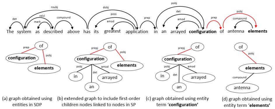
Figure 1: (a). Dependency graph for the example sentence; (b) to (e) Various sub-graphs obtained from the dependency graph for the sentence.

Although GCNs are useful for relation extraction, providing the appropriate graph structure with important vertices and edges is vital to achieve optimum performance. While using small-sized graphs would eliminate useful information from graphs, large-sized graphs can add more noise, resulting in difficulties for the network to learn useful vertex representations. For example, while the Contextualised Graph Convolution Network (C-GCN) Zhang et al. (2018) achieves a higher performance with graphs using first-order child vertices connected to vertices in SDP (such as the ones shown in Figure 1(b)), it’s performance significantly drops when the graph is limited to the vertices in SDP (Figure 1(a)) or when a higher number of child vertices (second order and above) are included in the graph. inline, size=, caption=2do, ] This is the first mention of C-GCN. Give the full form. Contextualised Graph Convolutional Networks? Moreover, GCNs are known to struggle on large-sized graphs derived from real-world datasets such as protein structures Borgwardt et al. (2005) and HIV infected patients’ data Ragin et al. (2012); Zhang et al. (2016). The noisy nature of graphs involving complex vertex features and edges complicates the learning for GCNs. To address the problem of dealing with large and noisier graphs, Lee et al. (2018) proposed graph attention model (GAM) to learn to discriminate patterns confined to specific regions in the large graph. inline, size=, caption=2do, ] Use the newcite command to get the desired Author-Year format in ACL bst

With a focus to reduce complexity in learning from large graphs, we propose to use multiple sub-graphs as opposed to using a single graph with graphical networks. Specifically, we derive multiple sub-graphs from a single dependency tree for the task of relation extraction. We propose a novel method to obtain sub-graphs using vertices corresponding to the target entities in the sentence as shown in Figures 1(c) and 1(d). Thus, instead of using a larger graph such as the one shown in Figure 1(b), we propose to use multiple sub-graphs (shown in Figures 1(a), (c) and (d)) to jointly learn for relation extraction. Using such segregated structures would facilitate focusing on specific regions, useful for learning richer representations, particularly for the vertices corresponding to the target entities.

Further, more recently, graph attention networks (GATs) Veličković et al. (2017) are shown to achieve superior performance for vertex classification in graph structured data. In contrast to GCNs that aggregate neighbouring vertices as features to generate vertex representations, GATs attend over neighbourhood vertex features to compute weights for learning vertex representations. In this paper, we propose to use GATs for relation extraction. Although GATs Veličković et al. (2017) consider the importance of neighbouring vertices for deriving vertex representations, GATs do not consider the edge features for computing attention weights. Recently Gong and Cheng (2018) showed that by combining edge features with GATs improves vertex classification. In the context of relation extraction, edge features can provide useful clues to identify relations across entities. For example, the information of vertices connected to different entity types or the dependency relation between vertices can serve as useful features when computing the salience of neighbouring vertices. Given this aspect, we proposes a contextualised GAT that combines edge features for relation extraction. The key contributions of this paper are:

• Propose a contextualized graph attention network that combines edge features from multiple sub-graphs for relation extraction.

• Present a novel method to derive sub-graphs using dependency parse and entity positions.

• Combining dependency relations and entity type features with GATs and GCNs.

• Conduct an empirical comparison between graphical networks (GCNs and GAT) using single-graph vs. multiple sub-graphs.

Our proposed method achieves the state-of-the-art (SoTA) performance for relation extraction on the Semeval 2010 Task 8 relation extraction benchmark dataset.

2 Related Work

Various graph-based neural networks are shown to improve relation extraction. Xu et al. (2015) applied LSTMs over SDP between the target entities to generalise the concept of dependency path kernels. Liu et al. (2015) used RNNs to model sub-trees in the dependency graph and a CNN to capture salient features from the SDP. Miwa and Bansal (2016) used Tree-LSTMs Tai et al. (2015) and BiLSTMs on dependency tree structures to jointly model entity and relation extraction. Zhang et al. (2018) proposed C-GCNs for relation and proposed a pruning strategy to selectively include vertices in the graph structure. Guo et al. (2019) presented Contextual-Attention Guided Graph Convolutional Networks (C-AGGCN) to selectively attend to important parts in the dependency graph to learn rich node representation in the graphical network. inline, size=, caption=2do, ] First mention of C-AGGCN. Give the full form name within brackets when you introduce an acronym for the first time. On the other hand, the key focus of this paper is to combine multiple sub-graphs for relation extraction as opposed to learning from a single graph as in the case of C-GCN and C-AGGCN. For this purpose, we modify GAT Veličković et al. (2017) and incorporate novel edge features for relation extraction. To the best knowledge of the authors, this is the first study that proposes a contextualised graph attention network with edge features, to learn from multiple sub-graphs for improved relation extraction. inline, size=, caption=2do, ] Although not limited to this paper, I prefer writing each sentence in a separate line in LaTeXsource.That makes commenting out and editing easier, and also shows the logical structure of the text more clearly.

3 Contextualised Graph Attention with Edge Features over Multiple Graphs

3.1 Problem Formulation

Let $\mathcal{S}=[s_{1},...,s_{k}]$ denote a set of sentences, where each sentence $s_{i}=[x_{1},...x_{n}]$ is a set of tokens where $x_{i}$ is the $i$-th token. Further, each $s_{i}$ also consists of two target entities $e_{1}$ and $e_{2}$ between which a semantic relation $r$ exists, selected from a pre-defined set of relations $\mathcal{R}$. Thus, given $s_{i},e_{1}$ and $e_{2}$, the relation extraction task is to identify the relation $r$ that holds between entities $e_{1}$ and $e_{2}$. The set $\mathcal{R}$ also contains the label “no relation”, which is predicted when there exists no relation between the two entities. In this study, we formulate the relation extraction task as a graph classification task. For this purpose, each $s_{i}$ is represented as a set of sub-graphs $g_{i}^{k}$, where $k$ is the number of sub-graphs. Numerous operations are performed on the individual sub-graphs using a contextualised graph attention that combines edge features to learn rich vertex representations for relation extraction. The architecture of the proposed model is shown in Figure 2 and is further explained below.

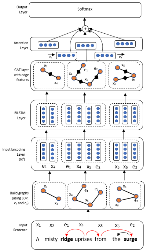
Figure 2: Architecture of the contextualised graph attention network incorporating edge features and conduct relation extraction using multiple sub-graphs.

3.2 Modelling Sentences using Sub-Graphs

The sentence $s_{i}$ and entity mentions $e_{1}$ and $e_{2}$ are provided as the input to the proposed model as seen in Figure 2. inline, size=, caption=2do, ] We already defined token sequence in the previous section. So I dropped it. In the first step, multiple sub-graphs for a sentence is created using the dependency parse of the sentence. Specifically, three sub-graphs are obtained using SDP and positions of the target entities $e_{1}$ and $e_{2}$. For instance, for the example sentence in Figure 2, the following three sub-graphs are obtained: (a) graph comprising vertices (“ridges”, “uprises”, “from”, “surge”) in SDP; (b) graph comprising vertices (“ridges”, “uprises”) connected to the entity $e_{1}$; (c) graph comprising vertices (“surge”, “from”, “the”) connected to the entity $e_{2}$. Although dependency parse defines the direction between related words, it is ignored to obtain undirected sub-graphs for the sentence as seen in Figure 2. We separately create an adjacency matrix $(\mathbf{A}^{k})$ to preserve the ordering of vertices. inline, size=, caption=2do, ] How is this matrix created?

$$s_{i}={g_{i}^{k}},\quad\mbox{ where}\>k=1,2,3$$ (1)

inline, size=, caption=2do, ] Use the align enviornment instead of equation and eqnarray environments for math.

3.3 Input encoding layer

Each sub-graph $g_{i}^{k}$ consists of a sequential set of tokens $[x_{1}^{k},\ldots,x_{n}^{k}]$ (although some words could be missing), which is encoded into a fixed length vector using (a) contextual; (b) part-of-speech; (c) dependency; (d) named entity type; and (e) word type embeddings. BERT Devlin et al. (2018) is used to obtain the contextual embeddings. BERT tokenises each token $x_{i}$ into $s$ Byte-Pair Encoding (BPE; Sennrich et al., 2016) tokens ($x_{i}=\{b_{1},b_{2},\ldots,b_{s}\}$) and generates $L$ hidden states for each BPE token, $\mathbf{h}_{t}^{l},1\leq l\leq L,1\leq t\leq s$. The contextual embedding for each token is obtained by summing the last four layers of the BERT model. Thus, the token encoding, $\mathbf{BERT}_{x_{i}}$ of the token $x_{i}$ is given by (2).

$$\mathbf{BERT}_{x_{i}}=\sum_{l=L-4}^{L}\frac{\sum_{t=1}^{s}\mathbf{h}_{t}^{l}}{s}.$$ (2)

Additionally, for each token $x_{i}$, a $p$-dimensional feature vector is created to represent (a) Part-of-Speech (POS) tags ($f_{x_{i}}^{pos}$); (b) dependency relations ($f_{x_{i}}^{dep}$); and (c) and named entity types ($f_{x_{i}}^{net}$). Moreover, a $q$-dimensional feature vector is created to indicate whether the token $x_{i}$ is an entity mention or not ($f_{x_{i}}^{wt}$). Thus, the final input vector for each token $x_{i}$ is given by (3).

$$\tilde{x}_{i}^{k}=[\mathbf{BERT}_{x_{i}^{k}};f_{x_{i}^{k}}^{pos};f_{x_{i}^{k}}^{dep};f_{x_{i}^{k}}^{net};f_{x_{i}^{k}}^{wt}]$$ (3)

$f_{x_{i}}^{pos}$, $f_{x_{i}}^{dep}$, $f_{x_{i}}^{net}$ and $f_{x_{i}}^{wt}$ are randomly initialised and updated during training, whereas $\mathbf{BERT}_{x_{i}}$ is computed according to (2) using a pre-trained BERT model. inline, size=, caption=2do, ] I added the last line as there was no mention as to how we get these additional embeddings. Did I say that correctly?

3.4 Contextual BiLSTM layer

To further fine-tune the input embeddings, the encoded series of input vectors $[\tilde{x}_{1}^{k},\ldots,\tilde{x}_{n}^{k}]$ in each graph is provided as the input to a contextualised BiLSTM layer to produce a $d^{l}$-dimensional hidden state vector for each input token in both forward and backward directions as given in (4).

$$\mathbf{\boldsymbol{h}}_{1}^{k},\ldots,\mathbf{\boldsymbol{h}}_{n}^{k}=\mathbf{BiLSTM}(\tilde{x}_{1}^{k},\ldots,\tilde{x}_{n}^{k})$$ (4)

Here, $\mathbf{h}_{i}\in\mathbb{R}^{2d^{l}}$, where $d^{l}$ is the dimension of hidden state of the LSTM and $\mathbf{h}_{i}$ is the hidden state vector of BiLSTM at time-step $i$, considering both forward and backward directions. The BiLSTM layer is jointly trained along with the rest of the model.

3.5 Graph Attention Layer with Edge Weights

Veličković et al. (2017) proposed GATs to assign larger weights to important vertices in the graph by computing attention weights across neighbouring vertices. inline, size=, caption=2do, ] We defined the acronym of GAT already in the intro. Do not define the same acronym multiple times in the same paper We modify the GAT to include the following edge features to compute attention weights for deriving vertex features in each sub-graph.

3.5.1 Edge Features

In addition to neighbouring vertices, edge features are useful for learning rich vertex representations, particularly in the context of relation extraction. For example, the information of vertices in the graph that are connected to entity mentions are helpful in providing higher weights for vertices connected to entity mentions to facilitate accurate relation extraction. Similarly, dependency relations between vertices can serve as useful features to improve relation extraction. Given the usefulness of edge features, we evaluate the following two types of edge features in combination with GAT.

Dependency relations based edge features (dref):

The dref features are derived based on the frequency of the dependency relations that exist between vertices in the training corpus as follows. Let $\mathcal{D}$ and $\mathcal{P}$ be the sets of respectively all dependency relations across vertices and Part-Of-Speech (POS) tags of vertices observed in the training corpus. The edge weight for a given dependency relation $r^{d}\in\mathcal{D}$ between vertices $i$ and $j$ with respectively POS tags $\lambda$ and $\mu\in\mathcal{P}$ ($\lambda=\mu$, where vertices $i$ and $j$ have the same POS tag) is defined as the ratio of total number of times the triple $(\lambda,\mu,r^{d})$ is encountered in the corpus to the total number of triples across all vertices (POS tags) with different dependency relations in the corpus. Each of these edge weights is assigned an $d^{e}$-dimensional random feature vector and subsequently updated along with the GAT in order to compute attention weights for deriving vertex representations. inline, size=, caption=2do, ] I replaced $p$ and $q$ as these were used previously for the dimensions of the feature vectors.

Connection type edge features (ctef):

The ctef features are used to identify whether a given node is connected to an entity term or a non-entity term in the graph. Because GCNs and GATs operate on undirected graphs, such information is not available to the network and providing information about vertices connected to entities can improve performance. Thus, a $d^{e}$-dimensional feature vector of ones is defined for edges where the out-going node is an entity mention, or a $d^{e}$-dimensional feature vector of zeros is included otherwise, and combined along with the GAT for computing vertex representations.

3.5.2 Graph Attention Operation

The output from the contextual BiLSTM layer combined with edge features (defined above) is provided as input to the GAT layer to produce a new set of $m$-dimensional vertex representations. inline, size=, caption=2do, ] We used $f$ above for feature vectors. Can we use a different symbol? $m$ for example? Following Veličković et al. (2017), to derive higher-level features from the input features, a shared linear transformation, parametrised by a weight martix, $\text{\bf W}\in\mathbb{R}^{{2d^{l}}\times m}$, is applied to every vertex. In order to perform self-attention on vertices, a shared attention mechanism $\alpha:\mathbb{R}^{m+{d^{e}}}\times\mathbb{R}^{m+{d^{e}}}\rightarrow\mathbb{R}$ is used to compute the attention coefficients, $e_{ij}$, that indicate the importance of vertex $j$’s features to vertex $i$ as given in (5).

$$e_{ij}=\alpha(\mathbf{W}\boldsymbol{h}_{i},\mathbf{W}\boldsymbol{h}_{j},\boldsymbol{e}_{ij}^{f})$$ (5)

Here, $\boldsymbol{e}_{ij}^{f}$ is $d^{e}$-dimension edge feature vector connecting vertex $j$ to vertex $i$, obtained as described earlier. The graph structure is injected into the attention mechanism by computing $e_{ij}$ for vertices $j\in\mathcal{N}_{i}$, where $\mathcal{N}_{i}$ is some neighbourhood of the vertex $i$ in the graph. The coefficients are normalised across all choices of $j$ using the softmax function to make them comparable across different vertices as given by (6).

$$\alpha_{ij}=\mathrm{softmax}_{j}(e_{ij})=\frac{\exp(e_{ij})}{\sum_{k\in\mathcal{N}_{i}}\exp(e_{ik})}$$ (6)

The attention mechanism, $\alpha$, is a single-layer feed-forward network, parametrised by a weight vector $\boldsymbol{\mathbf{\alpha}}\in\mathbb{R}^{m+{d^{e}}}$. Applying a non-linearity function, the attention coefficients is given by (7).

$$\alpha_{ij}=\frac{\exp(\mbox{L}(\boldsymbol{\alpha}{}^{\top}[\mathbf{W}\boldsymbol{h}_{i}\oplus\mathbf{W}\boldsymbol{h}_{j}\oplus\boldsymbol{e}_{ij}^{f}]))}{\sum_{k\in\mathcal{N}_{i}}\exp(\mbox{L}(\boldsymbol{\alpha}{}^{\top}[\mathbf{W}\boldsymbol{h}_{i}\oplus\mathbf{W}\boldsymbol{h}_{j}\oplus\boldsymbol{e}_{ij}^{f}]))}$$ (7)

Here, L is the LeakyReLU non-linearity function with negative slope $\alpha=0.2$, ^⊤ is transposition and $\oplus$ denotes vector concatenation. inline, size=, caption=2do, ] —— is used in vector norm. $\oplus$ is better The normalised attention coefficients considering adjacent vertex and edge features are linearly combined with corresponding vertex features to obtain the final output representation for each vertex as given by (8).

$$\boldsymbol{h}_{i}^{l}=\sigma\left(\sum_{j\in\mathcal{N}}\alpha_{ij}\mathbf{W}\boldsymbol{h_{j}}\right)$$ (8)

Veličković et al. (2017) found that extending the attention mechanism to multi-head attention was further beneficial for vertex classification. Consequently, we use multi-head attention on the combination of vertex and edge features. Specifically, the transformation given by (8) is executed $K$ independent times and the resulting features are concatenated to obtain the vertex representation in (9) for individual vertices.

$$\boldsymbol{h}_{i}^{l}=\bigoplus_{k=1}^{K}\sigma\left(\sum_{j\in\mathcal{N}}\alpha_{ij}^{k}\mathbf{W^{k}}\boldsymbol{h_{j}}\right)$$ (9)

3.6 Attention layer

The output of the graph attention layer combined with edge features is the vertex-level output $\mathbf{Z}\in\mathbb{R}^{n\times m}$, where $n$ is the number of nodes and $m$ is the dimensionality of the output features. Intuitively, the feature representation of each vertex is an aggregation of information from the connecting neighbouring vertices and edge features in the graph. In order to derive the final representation to be used for relation classification, a final attention layer is used to determine each vertex’s contribution and derive a fixed-length feature vector for the graph $g_{i}$. The attention mechanism in the final attention layer assigns a weight $\alpha^{\prime}_{i}$ to each vertex annotation $\boldsymbol{h}_{i}^{l}$. A fixed-length representation $v_{g_{i}}\in\mathbb{R}^{d^{g}}$ is computed for the graph $g_{i}$, as the weighted-sum of all vertex annotations as given by (10).

$$v_{g_{i}} =\sum_{i=1}^{N}\alpha^{\prime}_{i}\boldsymbol{h}_{i}^{l},\ \ \ v_{g_{i}}\in\mathbb{R}^{d^{g}}$$ (10)

$$\text{where, }u_{i} =\tanh(\text{\bf W}^{\prime}\boldsymbol{h}_{i}^{l})$$ (11)

$$\alpha^{\prime}_{i} =\frac{\exp(u_{i})}{\sum_{t=1}^{T}\exp(u_{t})},\mbox{ }\sum_{i=1}^{T}\alpha_{i}=1$$ (12)

Here, $\alpha^{\prime}_{i},\text{\bf W}^{\prime}$ indicate the parameters of the attention layer on top of GAT. The final representation for the sentence is obtained by summing all the three vectors obtained for the three graphs along with the corresponding hidden state vectors of entity mentions $e_{1}$ and $e_{2}$ obtained at the GAT layer as given by (13).

$$v=\sum_{i=1}^{2}\boldsymbol{h}_{e_{i}}^{l}+\sum_{k=1}^{3}v_{g_{i}^{k}},\mbox{ }h_{e_{i}}^{l}\in\mathbb{R}^{d^{g}},\text{ }v_{g_{i}^{k}}\in\mathbb{R}^{d^{g}}$$ (13)

Here, $\boldsymbol{h}_{e_{i}}^{l}$ is the hidden state vector of entity mentions $e_{i}$ at layer $l$ of GAT.

3.7 Output Layer

The final feature vector from attention layer $v\in\mathbb{R}^{d^{g}}$ is provided as input to a fully connected softmax layer to obtain a probability distribution over relation types. The cross-entropy loss for label prediction is given by (14).

$$J(\theta)=\sum_{i=1}^{r}\log p(r_{q}|v,\theta)$$ (14)

Here, $r$ is the total number of relation types and $\theta$ are the parameters of the model. During inference, the test instances are represented as graphs and fed to the trained classifier to predict the corresponding relation type.

4 Experiments

4.1 Dataset

We evaluate the proposed method on the SemEval-2010 Task 8 dataset (SemEval), which contains 10,717 sentences (8,000 train and 2,717 test), with each sentence marked with two nominals ($e_{1}$ and $e_{2}$) and labelled with a relation $r$ from a set of 9 different relation types and an artificial relation “Other”. The task is to predict the relation between the nominals considering the directionality. Following prior work, we report the official macro F1-Score excluding the ‘Other’ relation as the evaluation measure.

4.2 Implementation Details

The proposed model is implemented using PyTorch. Spacy Honnibal and Montani (2017) is used to obtain dependency trees, POS tags, named entity types, and dependency relations. PyTorch Geometric (PyG; Fey and Lenssen, 2019), is used to implement GCN and GAT with combined edge features. The hyperparameters of the model were tuned using a development set obtained by randomly selecting 10% of the training set. inline, size=, caption=2do, ] It is obvious you tested on the test set. I removed test set from that sentence because that sentence is about hyperparameter tuning The model was trained for 200 iterations following mini-batch gradient descent (SGD) with a batch size of 50. Word embeddings were initialised using 768-dimensional contextual BERT embeddings. The dimensions for embeddings for part-of-speech (POS), named entity tags, dependency tags was set to 40 and were initialised randomly. The dimensions for word-type embeddings was set to 10. The dimensions of hidden state vector in the LSTM, GCN, GAT and attention layer was set to 256.

4.3 Evaluated Models

Given the two types of edge features used in this study (described in section 3.5.1), the contextualised graph attention network over multiple graphs (c+gat+mg) using different sets of edge features: c+gat+mg+dref; c+gat+mg+ctef; c+gat+mg+dref+ctef are evaluated against various baseline models as listed in Table 1.

(1) c+gat+mg with out edge features;
(2) gat using multiple graphs with different edge features: gat+mg; gat+mg+ctef; gat+mg+dref; gat+mg+ctef+dref;
(3) gat using single graph with different edge features: gat+sg; gat+sg+ctef; gat+sg+dref; gat+sg+ctef+dref;
(4) contextualized gcn using multiple graphs with various edge features: c+gcn+mg; c+gcn+mg+ctef; c+gcn+mg+dref; c+gcn+mg+ctef+dref;
(5) contextualized gcn using single graph with different edge features: c+gcn+sg; c+gcn+sg+ctef; c+gcn+sg+dref; c+gcn+sg+ctef+dref;
(6) gcn using multiple graphs with various edge features: gcn+mg; gcn+mg+ctef; gcn+mg+dref; gcn+mg+ctef+dref;
(7) gcn using single graph with various edge features: gcn+sg; gcn+sg+ctef; gcn+sg+dref; gcn+sg+ctef+dref.

Table 1: Various baselines evaluated in the study

inline, size=, caption=2do, ] I removed the subsection to get space and avoid subsubsections

4.4 Influence of Edge Features

The performance of various models using different sets of vertex features is shown in Table 2. The c+gat+mg+dref model using dependency relation-based edge features achieves the best F1-score of 86.30. The c+gat+mg+dref model scores both in terms of higher precision (86.03) and recall (86.66) to achieve a higher F1-score, indicating the usefulness of the proposed model. The GCN models using dref and ctef edge features also report comparatively higher F1-scores of 85.82 and 85.91, respectively. The higher performance of c+gat+dref model mainly due to its higher recall (87.56). However, c+gat+ctef scores a higher precision (87.24) using ctef features.

As clearly evident from Table 2, combining edge features along with vertex features generally helps to obtain superior performance in comparison to models that rely only on vertex features. For example, the performance of c+gat+mg model using both vertex features and edge features (ctef and dref) is higher than that of c+gat+mg, which considers only vertex features. A similar result is observed across other multiple graph-based models such as gat+mg, c+gcn+mg and gcn+mg. Although a higher performance is achieved using dref and ctef edge features individually, combining dref and ctef does not help in further improving the performance.

We see that using a contextual layer to provide vertex features for GCN and GAT layers is useful for obtaining better performance. As seen in Table 2, both GCN and GAT models using a contextual layer achieve higher F1-scores over their non-contextual counterparts for both single and multiple sub-graphs. The performance of GAT-based models is comparatively higher than GCN-based models for relation extraction. The ability of GATs to attend to neighbouring vertices and edge features when computing vertex representations is more useful than simply considering the structural information as in the case of GCNs to achieve higher performance.

Model	P	R	F
single graph (sg)
gcn+sg	81.82	79.44	80.50
gcn+sg+ctef	80.25	80.57	80.28
gcn+sg+dref	81.49	82.15	81.74
gcn+sg+ctef+dref	81.32	80.06	80.50
c+gcn+sg	83.16	84.62	83.84
c+gcn+sg+ctef	82.80	84.28	83.44
c+gcn+sg+dref	82.91	84.02	83.39
c+gcn+sg+ctef+dref	82.66	83.92	83.16
gat+sg	81.34	80.40	80.80
gat+sg+ctef	83.85	78.27	80.78
gat+sg+dref	81.92	81.44	81.63
gat+sg+ctef+dref	81.49	80.98	81.13
c+gat+sg	82.18	85.04	83.52
c+gat+sg+ctef	83.21	82.80	82.87
c+gat+sg+dref	82.28	83.72	82.89
c+gat+sg+ctef+dref	83.11	82.98	82.94
multiple graphs (mg)
gcn+mg	83.18	85.89	84.40
gcn+mg+ctef	87.97	82.49	84.99
gcn+mg+dref	84.39	84.76	84.52
gcn+mg+ctef+dref	85.57	84.04	84.74
c+gcn+mg	86.28	83.63	84.83
c+gcn+mg+ctef	87.24	84.65	85.82
c+gcn+mg+dref	84.43	87.56	85.91
c+gcn+mg+ctef+dref	83.53	88.08	85.40
gat+mg	86.08	83.76	84.80
gat+mg+ctef	84.98	84.33	84.61
gat+mg+dref	85.37	85.06	85.16
gat+mg+ctef+dref	85.37	85.06	85.16
c+gat+mg	86.84	83.64	85.12
c+gat+mg+ctef	86.60	84.85	85.62
c+gat+mg+dref	86.03	86.66	86.30
c+gat+mg+ctef+dref	84.94	85.53	85.16

Table 2: Performance of various models on SemEval test set. P: Precision; R: Recall; F: F1-score

inline, size=, caption=2do, ] Use booktabs for nicer tables

4.5 Using Single vs. Multiple Graphs

It is evident from Table 2 that by using multiple sub-graphs instead of a single graph is beneficial for relation extraction. The performance of gcn, c+gcn, gat and c+gat models using multiple graphs scores significantly higher than its counterparts using only a single graph. The improvement is not limited to models that use edge features but holds true for models that do not use edge features as well. For example, results of c+gat+mg (F1-score of 85.12), which uses multiple sub-graphs (without edge features) is higher than c+gat+sg (F1-score of 83.52), which uses a single graph. The same results can be seen across other models: gat+mg (84.80) vs. gat+sg (80.80); c+gcn+mg (84.83) vs. c+gcn+sg (83.84) and gcn+mg (84.40) vs. gcn+sg (80.50). The above results sufficiently establish that using segregated smaller sub-graphs as opposed to a single graph is more useful in learning richer vertex representations for relation extraction.

4.6 Effect of Sentence Span

To further assess the contribution of multiple sub-graphs over a single graph, we compare their performances using sentences with different lengths. For this purpose, we divide the SemEval test set into three groups (Table 3, $\mu=3,\sigma=9$) based on the distance between $e_{1}$ and $e_{2}$: (1) short spans $(k\leq\mu-\sigma)$; (2) medium spans $(\mu-\sigma<k<\mu+\sigma)$; and (3) long spans $(k\geq\mu+\sigma)$, where $\mu$ is the average number of tokens, and $\sigma$ is the standard deviation over different lengths of tokens ($k$) between $e_{1}$ and $e_{2}$.

Short	Medium	Long	Total
365	1966	386	2717
13.50 (%)	72.30 (%)	14.20 (%)

Table 3: Total number of spans of different lengths and their percentage shares.

The best performing models using single graph (c+gat+sg) and multiple graphs (c+gat+mg) were examined on sentences in the above three categories as shown in Table 4. Interestingly, as seen in Table 4, different models using multiple graphs achieve a significantly higher performance than models using a single graph on sentences in the short span category. While c+gat+mg model without edge features, using a single graph achieves an F1-score of 73.09, the same model using multiple sub-graphs achieves an F1-score of 80.07. Although short span sentences form about 13.50% of total sentences in the test set (Table 3), a significant improvement in the performance of models using multiple graphs on short spans contributes in achieving a higher score in the overall performance. The performance of models using multiple sub-graphs is also equally higher on long span sentences in comparison to models using a single graph. The ability of different models using multiple graphs to achieve a higher performance even in without edge features clearly shows that using multiple graphs with graph-based models is a useful method for relation extraction.

Model	P (%)	R (%)	F (%)
Models using Single Graph
	short spans
c+gat+sg	73.07	74.85	73.09
c+gat+sg+ctef	75.28	76.86	75.48
c+gat+sg+dref	73.93	73.97	73.34
c+gat+sg+ctef+dref	75.97	76.69	75.56
	medium spans
c+gat+sg	84.01	86.95	85.42
c+gat+sg+ctef	84.75	84.33	84.43
c+gat+sg+dref	83.50	85.14	84.24
c+gat+sg+ctef+dref	84.22	84.42	84.26
	long spans
c+gat+sg	72.12	75.62	73.69
c+gat+sg+ctef	74.47	73.70	73.85
c+gat+sg+dref	76.06	78.56	76.98
c+gat+sg+ctef+dref	76.91	75.43	75.80
Models using Multiple Graphs
	short spans
c+gat+mg	83.18	78.90	80.07
c+gat+mg+ctef	83.15	78.32	79.92
c+gat+mg+dref	81.17	80.39	80.55
c+gat+mg+ctef+dref	86.03	82.45	83.93
	medium spans
c+gat+mg	87.83	84.94	86.27
c+gat+mg+ctef	87.77	86.24	86.94
c+gat+mg+dref	87.53	88.22	87.82
c+gat+mg+ctef+dref	85.65	87.22	86.36
	long spans
c+gat+mg	83.86	77.75	80.04
c+gat+mg+ctef	82.52	78.54	79.70
c+gat+mg+dref	77.37	80.25	78.43
c+gat+mg+ctef+dref	77.65	77.57	77.37

Table 4: Performance of models across short, medium and long spans in SemEval test set. P: Precision, R: Recall, F: F1-score

4.7 Influence of Graph Size

To evaluate the impact of graph size, we compare the performance of c-gat-mg-dref model under different graph sizes in Table 5. Therein, c+gat+mg+dref indicates a graph limited to vertices in SDP; c+gat+mg+dref_1 is where first-order child vertices connected to the vertices in SDP are added in the graph; and c+gat+mg+dref_2 is where second and higher order child vertices associated with the vertices in SDP are included in the graph. As seen from Table 5, the performance of c+gat+mg+dref model decreases with the graph size, indicating that distantly-connected vertices do not provide information relevant to the target relation.

Model	P	R	F
c+gat+mg+dref	86.03	86.66	86.30
c+gat+mg+dref_1	85.97	85.26	85.56
c+gat+mg+dref_2	84.81	86.04	85.36

Table 5: Performance of c+gat+dref+mg on different graph sizes. P: Precision; R: Recall; F: F1-score

4.8 Comparisons against State-of-the-art

The proposed c+gat+mg+dref model achieves the best F1-score of 86.3 against the SoTA graph-based models for relation extraction as shown in Table 6. The c+gat+mg+dref model scores higher than the C-AGGCN Guo et al. (2019) model that selectively attends to relevant sub-structures by considering the full dependency graph. Moreover, the GCN-based model (c-gcn-mg-dref) using multiple graphs achieves a higher F1-score of 85.9 compared to the C-GCN model Zhang et al. (2018), which scores an F1-score of 84.8 using a pruned dependency tree along with the GCN model.

Model Details	F1-Score
SVM Rink and Harabagiu (2010)	82.2
RNN Socher et al. (2012)	77.6
MVRNN Socher et al. (2012)	82.4
FCM Yu et al. (2014)	83.0
CR-CNN Santos et al. (2015)	84.1
SDP-LSTM Xu et al. (2015)	83.7
DepNN Liu et al. (2015)	83.6
PA-LSTM Zhang et al. (2017)	82.7
C-GCN Zhang et al. (2018)	84.8
SPTree Miwa and Bansal (2016)	85.5
C-AGGCN Guo et al. (2019)	85.7
our models
c-gcn-mg-dref	85.9
c-gat-mg-dref	86.3

Table 6: Performance of the proposed model against state-of-the-art graph-based models for relation extraction.

5 Conclusion

We proposed a contextualised graph attention network using edge features and operating on multiple sub-graphs for relation classification. The proposed sub-graph partition method learns rich vertex representations for relation classification. We proposed two sets of edge features using dependency relations and connecting entity types and showed that by combining such edge features with GAT we establish a new state-of-the-art on the SemEval relation classification benchmark dataset. The experimental results showed that using multiple sub-graphs is better than using a single graph with graphical networks such as GCNs and GATs.

References

- Borgwardt et al. (2005) Karsten M Borgwardt, Cheng Soon Ong, Stefan Schönauer, SVN Vishwanathan, Alex J Smola, and Hans-Peter Kriegel. 2005. Protein function prediction via graph kernels. Bioinformatics, 21(suppl_1):i47–i56.
- Devlin et al. (2018) Jacob Devlin, Ming-Wei Chang, Kenton Lee, and Kristina Toutanova. 2018. Bert: Pre-training of deep bidirectional transformers for language understanding. arXiv preprint arXiv:1810.04805.
- Fey and Lenssen (2019) Matthias Fey and Jan E. Lenssen. 2019. Fast graph representation learning with PyTorch Geometric. In ICLR Workshop on Representation Learning on Graphs and Manifolds.
- Fu et al. (2019) Tsu-Jui Fu, Peng-Hsuan Li, and Wei-Yun Ma. 2019. Graphrel: Modeling text as relational graphs for joint entity and relation extraction. In Proceedings of the 57th Annual Meeting of the Association for Computational Linguistics, pages 1409–1418.
- Gong and Cheng (2018) Liyu Gong and Qiang Cheng. 2018. Exploiting edge features in graph neural networks. arXiv preprint arXiv:1809.02709.
- Guo et al. (2019) Zhijiang Guo, Yan Zhang, and Wei Lu. 2019. Attention guided graph convolutional networks for relation extraction. arXiv preprint arXiv:1906.07510.
- Honnibal and Montani (2017) Matthew Honnibal and Ines Montani. 2017. spaCy 2: Natural language understanding with Bloom embeddings, convolutional neural networks and incremental parsing. To appear.
- Lee et al. (2018) John Boaz Lee, Ryan Rossi, and Xiangnan Kong. 2018. Graph classification using structural attention. In Proceedings of the 24th ACM SIGKDD International Conference on Knowledge Discovery & Data Mining, pages 1666–1674. ACM.
- Liu et al. (2015) Yang Liu, Furu Wei, Sujian Li, Heng Ji, Ming Zhou, and Houfeng Wang. 2015. A dependency-based neural network for relation classification. In Proceedings of the 53rd Annual Meeting of the Association for Computational Joint Conference on Natural Language Processing and the 7th International Joint Conference on Natural Language Processing, pages 285–290.
- Miwa and Bansal (2016) Makoto Miwa and Mohit Bansal. 2016. End-to-end relation extraction using lstms on sequences and tree structures. arXiv preprint arXiv:1601.00770.
- Peng et al. (2017) Nanyun Peng, Hoifung Poon, Chris Quirk, Kristina Toutanova, and Wen-tau Yih. 2017. Cross-sentence n-ary relation extraction with graph lstms. Transactions of the Association for Computational Linguistics, 5:101–115.
- Ragin et al. (2012) Ann B Ragin, Hongyan Du, Renee Ochs, Ying Wu, Christina L Sammet, Alfred Shoukry, and Leon G Epstein. 2012. Structural brain alterations can be detected early in hiv infection. Neurology, 79(24):2328–2334.
- Rink and Harabagiu (2010) Bryan Rink and Sanda Harabagiu. 2010. Utd: Classifying semantic relations by combining lexical and semantic resources. In Proceedings of the 5th International Workshop on Semantic Evaluation, pages 256–259. Association for Computational Linguistics.
- Santos et al. (2015) Cicero Nogueira dos Santos, Bing Xiang, and Bowen Zhou. 2015. Classifying relations by ranking with convolutional neural networks. In Proceedings of the 53rd Annual Meeting of the Association for Computational Linguistics and the 7th International Joint Conference, pages 626–634.
- Schlichtkrull et al. (2018) Michael Schlichtkrull, Thomas N Kipf, Peter Bloem, Rianne Van Den Berg, Ivan Titov, and Max Welling. 2018. Modeling relational data with graph convolutional networks. In European Semantic Web Conference, pages 593–607. Springer.
- Sennrich et al. (2016) Rico Sennrich, Barry Haddow, and Alexandra Birch. 2016. Neural machine translation of rare words with subword units. In Proceedings of the 54th Annual Meeting of the Association for Computational Linguistics (Volume 1: Long Papers), pages 1715–1725, Berlin, Germany. Association for Computational Linguistics.
- Socher et al. (2012) Richard Socher, Brody Huval, Christopher D Manning, and Andrew Y Ng. 2012. Semantic compositionality through recursive matrix-vector spaces. In Proceedings of the 2012 joint conference on empirical methods in natural language processing and computational natural language learning, pages 1201–1211. Association for Computational Linguistics.
- Tai et al. (2015) Kai Sheng Tai, Richard Socher, and Christopher D Manning. 2015. Improved semantic representations from tree-structured long short-term memory networks. arXiv preprint arXiv:1503.00075.
- Veličković et al. (2017) Petar Veličković, Guillem Cucurull, Arantxa Casanova, Adriana Romero, Pietro Lio, and Yoshua Bengio. 2017. Graph attention networks. arXiv preprint arXiv:1710.10903.
- Xu et al. (2015) Yan Xu, Lili Mou, Ge Li, Yunchuan Chen, Hao Peng, and Zhi Jin. 2015. Classifying relations via long short term memory networks along shortest dependency paths. In proceedings of the 2015 conference on empirical methods in natural language processing, pages 1785–1794.
- Yu et al. (2014) Mo Yu, Matthew Gormley, and Mark Dredze. 2014. Factor-based compositional embedding models. In NIPS Workshop on Learning Semantics, pages 95–101.
- Zhang et al. (2016) Jingyuan Zhang, Bokai Cao, Sihong Xie, Chun-Ta Lu, Philip S Yu, and Ann B Ragin. 2016. Identifying connectivity patterns for brain diseases via multi-side-view guided deep architectures. In Proceedings of the 2016 SIAM International Conference on Data Mining, pages 36–44. SIAM.
- Zhang et al. (2018) Yuhao Zhang, Peng Qi, and Christopher D Manning. 2018. Graph convolution over pruned dependency trees improves relation extraction. arXiv preprint arXiv:1809.10185.
- Zhang et al. (2017) Yuhao Zhang, Victor Zhong, Danqi Chen, Gabor Angeli, and Christopher D Manning. 2017. Position-aware attention and supervised data improve slot filling. In Proceedings of the 2017 Conference on Empirical Methods in Natural Language Processing, pages 35–45.