Instability of the regularized 4D charged Einstein-Gauss-Bonnet de-Sitter black hole

Abstract

We studied the instability of the regularized 4D charged Einstein-Gauss-Bonnet de-Sitter black holes under charged scalar perturbations. The unstable modes satisfy the superradiant condition, but not all modes satisfying the superradiant condition are unstable. The instability occurs when the cosmological constant is small and the black hole charge is not too large. The Gauss-Bonnet coupling constant makes the unstable black hole more unstable when both the black hole charge and cosmological constant are small, and makes the stable black hole more stable when the black hole charge is large.

Department of Physics and Siyuan Laboratory, Jinan University, Guangzhou 510632, China

1 Introduction

It is known that general relativity should be modified from both the viewpoint of theory and observation. For examples the general relativity can not be renormalized and can not explain the dark side of the Universe. On the other hand, the Lovelock theorem states that in four dimensional vacuum spacetime, the general relativity with a cosmological constant is the unique metric theory of gravity with second order equations of motion and covariant divergence-free [1]. Beyond general relativity, one must go to higher dimensional spacetime, or add extra fields, or allow higher order derivative of metric or even abandon the Riemannian geometry. Various modified gravity theories have been proposed [2]. In this work, we focus on the Einstein-Gauss-Bonnet (EGB) gravity. The EGB gravity is one of most promising candidates of modified gravity. It has second order equations of motion and free of Ostrogradsky instability [3]. It appears naturally in the low energy effective action of heterotic string theory [4]. However, the Gauss-Bonnet (GB) term has nontrivial dynamics only in higher dimensions in general. In four dimensional spacetime, it is a topological term and does not contribute to the dynamics. By rescaling the GB coupling constant in a special way, novel four dimensional GB black hole solution was found recently [5]. This work provides a new classical four dimensional gravity theory and has inspired many studies, including the new black hole solutions [6, 7, 8], perturbations [9, 10, 11, 12], shadow and geodesics [13], thermodynamics [14], and other aspects [15, 16].

The novel black hole solution has some remarkable properties. Its singularity at the center is timelike. The gravitational force near the center is repulsive and the free infalling particles can not reach the singularity [5]. One may expect that the novel black hole solution would also show some new properties under perturbations, and some related works have been done [9, 11]. The study of the stability of black hole is an active area in black hole physics. It can be used to extract the parameters of the black hole such as its mass, charge and angular momentum. The stability of black hole is also related to gravitational wave, black hole thermodynamics, information paradox and holography, etc. [17]. Among these studies, the stability of black hole in asymptotic de Sitter (dS) spacetime is intriguing. The Kerr black hole in dS spacetime also behaves very different with those in asymptotic spacetime under perturbations [18]. The four dimensional Reissner-Nordström-de Sitter (RN-dS) may violate the strong cosmic censorship [19, 20]. The higher dimensional RN-dS and Gauss-Bonnet-de Sitter (GB-dS) black holes are unstable [21, 22].

A quite surprising and still not very well understood result was discovered in [23, 24, 25], where they showed that RN-dS black hole is unstable under charged scalar perturbations. Such instability satisfies superradiance condition [26]. However, only the monopole $l=0$ suffers from this instability. Higher multipoles are stable. This is distinct from superradiance. To understand the precise mechanism, one may need the nonlinear studies, which was partially answered in recent works [20]. In this paper, we consider the instability of the novel 4D charged EGB black hole in asymptotic dS spacetime under charged scalar perturbations. We will see that the behavior is very different with the case in asymptotic flat spacetime which has been done in [11]. The Gauss-Bonnet coupling constant plays a more subtle role here.

The paper is organized as follows. Section 2 describes the novel 4D EGB-RN-dS black hole and gives the reasonable parameters region. Section 3 shows the charged scalar perturbation equations. Section 4 describes the numerical method we used and gives the results of the quasinormal modes. Section 5 is the summary and discussion.

2 The 4D charged EGB-dS black hole

The action of the EGB gravity with electromagnetic field in $D$-dimensional spacetime has the form

$$S=\frac{1}{16\pi}\int d^{D}x\sqrt{-g}\left[R+2\Lambda+\frac{\alpha}{D-4}\mathcal{G}^{2}-F_{\mu\nu}F^{\mu\nu}\right],$$ (2.1)

with $R$ the Ricci scalar, $g$ the determinant of the metric $g_{\mu\nu}$, and $\Lambda$ the positive cosmological constant. The Maxwell tensor $F_{\mu\nu}=\partial_{\mu}A_{\nu}-\partial_{\nu}A_{\mu}$, in which $A_{\mu}$ is the gauge potential. The Gauss-Bonnet term

$$\mathcal{G}^{2}=R^{2}-4R_{\mu\nu}R^{\mu\nu}+R_{\mu\nu\alpha\beta}R^{\mu\nu\alpha\beta}=\frac{1}{4}\delta_{\rho\sigma\gamma\delta}^{\mu\nu\alpha\beta}R_{\ \ \mu\nu}^{\rho\sigma}R_{\ \ \alpha\beta}^{\gamma\delta},$$ (2.2)

with $R_{\mu\nu}$ the Ricci tensor and $R_{\mu\nu\alpha\beta}$ the Riemann tensor. We have rescaled the Gauss-Bonnet coupling constant $\alpha$ by a factor $\frac{1}{D-4}$ in (2.1).

Varying the action with respect to the metric, one gets the equation of motion

$$G_{\mu\nu}+\frac{\alpha}{D-4}H_{\mu\nu}=T_{\mu\nu}+\Lambda g_{\mu\nu}.$$ (2.3)

Here $G_{\mu\nu}$ is the Einstein tensor and the contribution from the GB term is given by

$$H_{\mu\nu}=2(RR_{\mu\nu}-2R_{\mu\sigma}R_{\ \nu}^{\sigma}-2R_{\mu\sigma\nu\rho}R^{\sigma\rho}-R_{\mu\sigma\rho\beta}R_{\ \ \ \nu}^{\sigma\rho\beta})-\frac{1}{2}g_{\mu\nu}\mathcal{G}^{2}.$$ (2.4)

In general, $H_{\mu\nu}$ vanishes in four dimensional spacetime and does not contribute to the dynamics. However, it was argued that the vanishing of $H_{\mu\nu}$ in four dimension might be canceled by the rescaled GB coupling constant $\frac{\alpha}{D-4}$, and new solutions were found [5]. The energy-momentum tensor of the Maxwell field in (2.3) takes the form

$$T_{\mu\nu}=\frac{1}{4}\left(F_{\mu\sigma}F_{\ \nu}^{\sigma}-\frac{1}{4}g_{\mu\nu}F_{\alpha\beta}F^{\alpha\beta}\right).$$ (2.5)

In spherical symmetric spacetime, the electrovacuum solution of (2.3) can be written as

$$ds^{2}=-f(r)dt^{2}+\frac{1}{f(r)}dr^{2}+r^{2}(d\theta^{2}+\sin^{2}\theta d\phi^{2}),$$ (2.6)

where the metric function

$$f(r)=1+\frac{r^{2}}{2\alpha}\left(1-\sqrt{1+4\alpha\left(\frac{M}{r^{3}}-\frac{Q^{2}}{r^{4}}+\frac{\Lambda}{3}\right)}\right),$$ (2.7)

and the gauge potential

$$A=-\frac{Q}{r}dt.$$ (2.8)

Here $M$ is the black hole mass and $Q$ the black hole charge. When $\alpha\to 0$, this solution returns to the RN-dS black hole. As $r\to\infty$, it gives the asymptotic dS spacetime with an effective positive cosmological constant. Note that the solution (2.6) coincides formally with the ones obtained from conformal anomaly and quantum corrections [27] and those from Horndeski theory [8].

The parameters $M$ and $Q$ are positive. The GB coupling constant $\alpha$ can be either positive or negative here. In appropriate parameter region, the solution has three horizons: the inner horizon $r_{-}$, the event horizon $r_{+}$ and cosmological horizon $r_{c}$. For negative $\alpha$, the metric function may not be real in small $r$ region. But since we are only interested in the region between $r_{+}$ and $r_{c}$, we allow negative $\alpha$ in this work. For convenience, hereafter we fix the black hole event horizon $r_{+}=1$. Then the mass parameter can be expressed as

$$M=1-\frac{\Lambda}{3}+Q^{2}+\alpha.$$ (2.9)

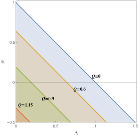
Figure 1: The parameter region that allows the event horizon $r_{+}$ and cosmological horizon $r_{c}$. The region is bounded by $Q^{2}+\alpha+\Lambda<1,$ $-0.5<\alpha$, $\Lambda>0$ and Q>0. As $Q$ increases, the allowed region for $(\Lambda,\alpha)$ shrinks. The extremal value of $Q=\sqrt{3/2}$.

Note that to ensure $f(1)=0$, there must be $\alpha>-1/2$. The parameter region where allows the black hole event horizon $r_{+}$ and the cosmological horizon $r_{c}$ can be determined by requiring $f^{\prime}(r_{+})>0$, which implies the black hole temperature is positive. This leads to

$$Q^{2}+\alpha+\Lambda<1.$$ (2.10)

This formula is very similar to the neutral case [10]. The final parameter region is shown in Fig. 1.

3 The charged scalar perturbation

It is known that fluctuations of order $\mathcal{O}(\epsilon)$ in the scalar field in a given background induce changes in the spacetime geometry of order $\mathcal{O}(\epsilon^{2})$ [26]. To leading order we can study the perturbations on a fixed background geometry. Let us consider a massless charged scalar field $\psi$ on the background (2.6). Its equation of motion is

$$0=D^{\mu}D_{\mu}\psi\equiv g^{\mu\nu}\left(\nabla_{\mu}-iqA_{\mu}\right)\left(\nabla_{\nu}-iqA_{\nu}\right)\psi,$$ (3.1)

where $q$ is the scalar charge and $\nabla_{\mu}$ the covariant derivative. For generic background, we can take the following decomposition

$$\psi=\sum_{lm}\int d\omega e^{-i\omega t}\frac{\Psi(r)}{r}Y_{lm}(\theta,\phi).$$ (3.2)

Here $Y_{lm}(\theta,\phi)$ is the spherical harmonics on the two sphere $S^{2}.$ The angular part and the radial part of the perturbation equation (3.1) decouple. What we are interested in is the radial part which can be written as the Schrödinger-like form

$$0=\frac{\partial^{2}\Psi}{\partial r_{\ast}^{2}}+\left(\omega^{2}-\frac{2qQ}{r}\omega-V_{\text{eff}}\right)\Psi,$$ (3.3)

where the tortoise coordinate $dr_{\ast}=dr/f$ is introduced. The effective potential reads

$$V_{\text{eff}}=-\frac{q^{2}Q^{2}}{r^{2}}+f\left(\frac{l(l+1)}{r^{2}}+\frac{\partial_{r}f}{r}\right).$$ (3.4)

Unlike to the case in asymptotic flat spacetime where only one potential barrier appears between $r_{+}$ and $r_{c}$, here a negative effective potential well may appear between $r_{+}$ and $r_{c}$. We will see that this potential well plays an important role in the instability of charged EGB-dS black hole under perturbations.

The radial equation has following asymptotic behavior near the horizons.

$$\Psi\to\begin{cases}e^{-i\left(\omega-\frac{qQ}{r_{+}}\right)r_{\ast}}\sim\left(r-r_{+}\right)^{-\frac{i}{2\kappa_{+}}\left(\omega-\frac{qQ}{r_{+}}\right)},&r\to r_{+},\\ e^{i\left(\omega-\frac{qQ}{r_{c}}\right)r_{\ast}}\sim\left(r-r_{c}\right)^{-\frac{i}{2\kappa_{c}}\left(\omega-\frac{qQ}{r_{c}}\right)},&r\to r_{c}.\end{cases}$$ (3.5)

Here $\kappa_{+}=\frac{1}{2f^{\prime}(r_{+})}$ is the surface gravity on the event horizon and $\kappa_{c}=-\frac{1}{2f^{\prime}(r_{c})}$ the surface gravity on the cosmological horizon. These asymptotic solution corresponds to ingoing boundary condition near the event horizon and outgoing boundary condition near the cosmological horizon. The system is dissipative and the frequency of the perturbations will be the composition of quasinormal modes (QNMs). With the specific boundary condition (3.5), the radial equation (3.3) can be solved as an eigenvalue problem. Only some discrete eigenfrequencies $\omega$ would satisfy both the radial equation and boundary condition. One can write the eigenfrequency as $\omega=\omega_{R}+i\omega_{I}$. When the imaginary part $\omega_{I}>0$, the amplitude of perturbation will grow exponentially and implies that the black hole is unstable at least in the linear perturbation level.

4 The instability of the 4D charged EGB-dS black hole

The radial equation (3.3) is generally hard to solve analytically, except in the regime where the frequency or the black hole size is very small [26, 28]. Many numerical method for QNMs calculations were thus developed, such as WKB method, shooting method, continued fraction method and Horowitz-Hubeny method [17]. Not all methods keeps high accuracy and efficiency in the charged case [29]. In this work, we adopt the asymptotic iteration method. Also, we testify our results from the asymptotic iteration methods with time evolution.

4.1 The asymptotic iteration method (AIM)

The asymptotic iteration method was used to solve the eigenvalues of the homogeneous second order ordinary derivative functions [30]. Later it was used to look for the quasinormal modes of black holes in asymptotic flat or (A)dS spacetime [31]. Let us first introduce an auxiliary variable

$$\xi=\frac{r-r_{+}}{r_{c}-r_{+}}.$$ (4.1)

It ranges from 0 to 1 as $r$ runs from the event horizon to the cosmological horizon. The radial equation (3.3) then becomes

$$0= \frac{\partial^{2}\Psi}{\partial\xi^{2}}\left(\frac{f}{r_{c}-r_{+}}\right)^{2}+\frac{\partial\Psi}{\partial\xi}\frac{f\partial_{\xi}f}{\left(r_{c}-r_{+}\right)^{2}}$$

$$+\left[\left(\omega-\frac{qQ}{(r_{c}-r_{+})\xi+r_{+}}\right)^{2}-f\left(\frac{l(l+1)+\left(\xi+\frac{r_{+}}{r_{c}-r_{+}}\right)\partial_{\xi}f}{\left[(r_{c}-r_{+})\xi+r_{+}\right]^{2}}\right)\right]\Psi.$$ (4.2)

The above equation is generally hard to solve analytically. We turn to the numerical method. In terms of $\xi$, the asymptotic solution near the horizons can be written as

$$\Psi\to \begin{cases}\xi^{-\frac{i}{2\kappa_{+}}\left(\omega-\frac{qQ}{r_{+}}\right)},&\xi\to 0,\\ \left(\xi-1\right)^{-\frac{i}{2\kappa_{c}}\left(\omega-\frac{qQ}{r_{c}}\right)},&\xi\to 1.\end{cases}$$ (4.3)

Then we can write the full solution of (4.2) satisfying the asymptotic behavior (4.3) in the following form

$$\Psi=\xi^{-\frac{i}{2\kappa_{+}}\left(\omega-\frac{qQ}{r_{+}}\right)}\left(\xi-1\right)^{\frac{i}{2\kappa_{c}}\left(\omega-\frac{qQ}{r_{c}}\right)}\chi(\xi).$$ (4.4)

Here $\chi(\xi)$ is a regular function of $\xi$ in range $(0,1)$ and obeys following homogeneous second order differential equation

$$\frac{\partial^{2}\chi}{\partial\xi^{2}}=\lambda_{0}(\xi)\frac{\partial\chi}{\partial\xi}+s_{0}(\xi)\chi,$$ (4.5)

in which the coefficients

$$-\lambda_{0}(\xi)=\frac{i\left(\omega-\frac{qQ}{r_{c}}\right)}{(\xi-1)\kappa_{c}}-\frac{i\left(\omega-\frac{qQ}{r_{+}}\right)}{\kappa_{+}\xi}+\frac{f^{\prime}(\xi)}{f(\xi)},\\$$ (4.6)

$$-s_{0}(\xi)= -\frac{\left(r_{c}-r_{+}\right)\left((\xi r_{c}-\xi r_{+}+r_{+})f^{\prime}(\xi)+l(l+1)\left(r_{c}-r_{+}\right)\right)}{f(\xi)\left((\xi-1)r_{+}-\xi r_{c}\right){}^{2}}$$ (4.7)

$$-\frac{\left(\omega-\frac{qQ}{r_{c}}\right)\left(\frac{\omega r_{c}-qQ}{2\kappa_{c}r_{c}}+i\right)}{2(\xi-1)^{2}\kappa_{c}}+\frac{\left(\omega-\frac{qQ}{r_{+}}\right)\left(\frac{qQ-r_{+}\omega}{2\kappa_{+}r_{+}}+i\right)}{2\kappa_{+}\xi^{2}}+\frac{\left(\omega-\frac{qQ}{r_{+}}\right)\left(\omega-\frac{qQ}{r_{c}}\right)}{2\kappa_{+}(\xi-1)\xi\kappa_{c}}$$

$$+\frac{if^{\prime}(\xi)\left(\omega-\frac{qQ}{r_{c}}\right)}{2(\xi-1)\kappa_{c}f(\xi)}-\frac{if^{\prime}(\xi)\left(\omega-\frac{qQ}{r_{+}}\right)}{2\kappa_{+}\xi f(\xi)}+\frac{\left(r_{c}-r_{+}\right){}^{2}\left(\omega-\frac{qQ}{\xi r_{c}-\xi r_{+}+r_{+}}\right){}^{2}}{f(\xi)^{2}}.$$

The coefficients $\lambda_{0}(\xi)$ and $s_{0}(\xi)$ are regular functions of $\xi$ in the interval $(0,1)$. Now using the same method described in [11], we can work out the quasinormal modes. We vary the iteration times and the expansion point to ensure the reliability of the results. The results are also checked by using other auxiliary variables such as $\xi=1-\frac{r_{+}}{r}$ or $\xi=\left(1-\frac{r_{+}}{r}\right)/\left(1-\frac{r_{+}}{r_{c}}\right)$. Except some extremal cases ($\Lambda\to 0$ or the black hole becomes extremal), they coincides well. Hereafter we set $q=1$ for convenience.

4.2 The eigenfrequencies of the charged scalar perturbation

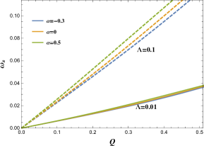
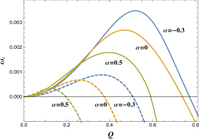
Figure 2: The real part (left) and imaginary part (right) of the fundamental modes of the QNMs when $l=0$. Solid lines for $\Lambda=0.01$, dashed lines for $\Lambda=0.1$

Let us first study the effects of the black hole charge $Q$ on the fundamental modes of the QNMs. It is shown in Fig. 2. From the left panel, we see that $\omega_{R}$ increases with $Q$ almost linearly. The slope is larger for larger $\Lambda$ and $\alpha$. In the right panel, $\omega_{I}$ increases with small $Q$ and then decreases with larger $Q$. For large enough $Q$, the black hole becomes stable. When $Q$ is small, positive $\alpha$ increases $\omega_{I}$ and negative $\alpha$ decreases $\omega_{I}$. This behavior is similar to the case in asymptotic flat spacetime [11] . However, when $Q$ is large, positive $\alpha$ decreases $\omega_{I}$ and negative $\alpha$ increases $\omega_{I}$. This is contrast with the cases in asymptotic flat spacetime. It implies that the positive GB coupling constant can make the black hole more unstable when the black hole charge $Q$ is small and more stable when $Q$ is large. Note further that no matter what values $\Lambda,\alpha$ take, when $Q\to 0$, both $\omega_{R}$ and $\omega_{I}$ tend to 0 from above. This implies the weakly charged black hole in dS spacetime is always unstable. The existence of $\alpha$ does not change this phenomenon qualitatively.

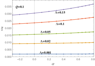
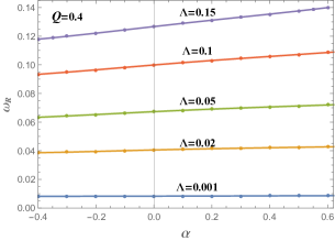
Figure 3: The real part of the fundamental modes of the QNMs when $l=0$. Left panel for $Q=0.1$, right panel for $Q=0.4$.

Now we study the effects of $\alpha$ on the fundamental modes in detail. Fig. 3 shows the real part of the fundamental modes $\omega_{R}$ when $Q=0.1$ and $Q=0.4$. For fixed $Q$, the real part $\omega_{R}$ increases almost linearly with $\alpha$ and $\Lambda$. Combining the results from Fig. 2, we conclude that $\omega_{R}\propto\alpha\Lambda Q$.

The behavior of the imaginary part of the fundamental modes $\omega_{I}$ is more interesting. In Fig. 4 we show the cases when $Q=0.1$ and $Q=0.4$. From the left and right panels, we see that $\omega_{I}$ increases with small $\Lambda$ and decreases with larger $\Lambda$. The effects of $\alpha$ on $\omega_{I}$ is subtle and relevant to the $\Lambda$ and $Q$. When both $Q$ and $\Lambda$ are small (left upper panel), $\omega_{I}$ increases with $\alpha$. For small $Q$ and larger $\Lambda$ (right upper panel), $\omega_{I}$ increases with $\alpha$ first and then decreases with $\alpha$. For larger $Q$ (lower panels), $\omega_{I}$ decreases with $\alpha$. This phenomenon is very different with the case in asymptotic flat spacetime [11], where $\alpha$ roughly increases $\omega_{I}$. This implies that the positive GB coupling constant $\alpha$ can suppress the instability of black hole. As $\alpha$ increase, it can even change the qualitative behavior of black hole under perturbations and render the unstable black hole stable.

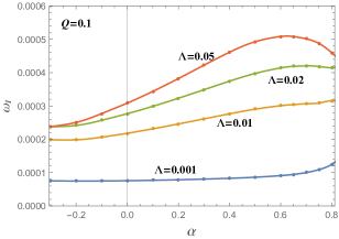
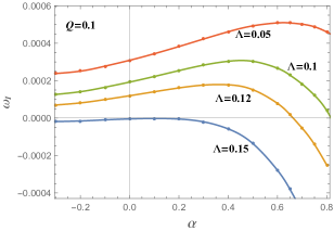
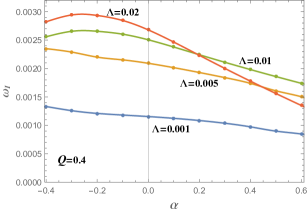
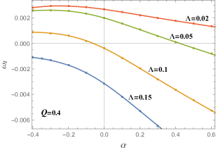
Figure 4: The imaginary part of the fundamental modes of the QNMs when $l=0$. The upper panel for $Q=0.1$, lower panel for $Q=0.4$. Left panel shows the cases for small $\Lambda$, the right panel for larger $\Lambda$.

The instability we found here is very reminiscent of superradiance. However, the case is subtle here. With the similar method used in [11, 24], one can show that superradiance occurs only when

$$\frac{qQ}{r_{+}}>\omega>\frac{qQ}{r_{c}}.$$ (4.8)

We see that some modes satisfying (4.8) are unstable, while there are indeed some modes satisfying (4.8) are stable. See Table 1 for evidence. In fact, as shown in [11, 24], the superradiant condition is the necessary but not sufficient condition for instability. The precise mechanism of the instability found here need more studies and will be addressed in section 5.

$\alpha$	$\frac{qQ}{r_{+}}$	$\frac{qQ}{r_{c}}$	$\omega$ (AIM)	$\omega_{I}$ (time domain)
0.5	0.1	0.0244042	0.0290311+0.0001514$i$	0.0001515
0.6	0.1	0.0248557	0.0297114+0.0000779$i$	0.0000780
0.65	0.1	0.0250987	0.0300692+0.0000191$i$	0.0000192
0.7	0.1	0.0253547	0.0304355–0.0000541$i$	-0.0000547
0.75	0.1	0.0256252	0.0308094–0.0001400$i$	-0.0001390

Table 1: The fundamental modes when $Q=0.1,\Lambda=0.12$ and $l=0$, which corresponds to the orange line in the upper right panel of Fig. 4. The last column is the imaginary part of the frequency extracted from the time evolution.

We also directly compute the time-evolution of the perturbation field $\psi$ to further reveal the instability of the 4D charged EGB-dS black hole. For time evolution, the Schrödinger-like equation becomes,

$$-\frac{\partial^{2}\Psi}{\partial t^{2}}-\frac{2iqQ}{r}\frac{\partial\Psi}{\partial t}+\frac{\partial^{2}\Psi}{\partial r_{*}^{2}}-V(r)\Psi=0,$$ (4.9)

In order to compute the time evolution of $\psi$ we adopt the discretization introduced in [23]. The reliability of this numerical method can be verified by the convergence of computations when increasing the sampling density. We impose the following initial profile,

$$\left\{\begin{aligned} \Psi(r_{*},t)&=0,&t<0,\\ \Psi(r_{*},t)&=\exp\left[{-\frac{(r_{*}-a)^{2}}{2b^{2}}}\right],&t=0.\end{aligned}\right.$$ (4.10)

The discretization of equation (4.9) is implemented in $(r_{*},t)$ plane. Also, we fix $\Delta t/\Delta r_{*}=0.5$ in order to satisfy the von Newmann stability conditions. Unlike some other analytical models where the $r_{*}$ can be solved analytically, here the $r_{*}(r)$ can only be obtained numerically. The $r_{*}(r)$ diverges as $\lim_{r\to r_{+}}\to-\infty$ and $\lim_{r\to r_{c}}\to\infty$, hence the error of the numerical $r_{*}(r)$ can be very large at the near horizon region. Therefore, we introduce a cutoff $\epsilon$ solve the $r_{*}(r)$ relation by solving the below system,

$$r_{*}^{\prime}(r)=1/f(r),\,r_{*}(r_{h}+\epsilon)=0,\,\text{with}\,r\in[r_{h}+\epsilon,r_{c}-\epsilon],$$ (4.11)

Usually the cutoff $\epsilon$ should not be too small, otherwise it leads to significant error of the resultant $r_{*}(r)$.

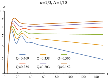
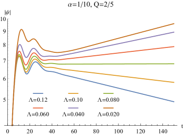
Figure 5: Left panel: the time evolution of the $|\psi(r_{*}=88.4216,t)|$ at $\alpha=2/3,\,\Lambda=1/10$, where each curve corresponds to different values of $Q$. Right panel: the time evolution of the $|\psi(r_{*}=88.4216,t)|$ at $\alpha=1/10,\,Q=2/5$, where each curve corresponds to different values of $\Lambda$. For both plots we fixed $a=88.4216,\,b=1/10$.

In order to obtain the late time evolution of the perturbation, we need to solve a large range or $r_{*}$. Since $1/f$ tends to diverge when $r\to r_{h}$ and $r\to r_{c}$, in near horizon region the $r_{*}(r)$ can be extracted analytically. A direct solution is to expand $1/f(r)$ with respect to $r_{h}$, because the horizon requires that $1/f(r)\sim 1/(r-r_{h})$. However, this direct expansion can lead to very large numerical error. A better solution is to expand $f(r)$ with respect to $r_{h}$, and then obtain the expansion of $1/f$ in terms of the expansion coefficients of the $f(r)$. After solving the analytical expansion coefficients, one may glue the analytical expansion in the near horizon region and the numerical solution of the $r_{*}(r)$ in $r\in[r_{h}+\epsilon,r_{c}-\epsilon]$. In this way, one may obtain a very large range of $r_{*}$ and a long-time evolution can be realized.

We show two examples of $|\psi(t)|$ in log plot in Fig. 5, from which we can see that $\ln|\psi|$ has linear dependence on $t$ for late time evolution. From the left panel of Fig. 5, when $Q$ is small the system is unstable ($\ln|\psi|$ linearly decreases with $t$), while for large values of $Q$ the system becomes stable ($\ln|\psi|$ linearly grows with $t$). This is in accordance with previous results of the frequency analysis (see the right panel of Fig. 2). From the right panel of Fig. 5 we see that when $\Lambda$ is small the system is unstable ($\ln|\psi|$ linearly increases with $t$), while for large values of $\Lambda$ the system becomes stable ($\ln|\psi|$ linearly decreases with $t$). This is in accordance with previous results of the frequency analysis (see the bottom right panel of Fig. 4).

It is also important to verify the validity of the asymptotic iteration method with the time evolution. Specifically, in the time evolution computation, we can extract the $\omega_{R}$ by computing the $\partial_{t}\ln(|\psi|)$ at late time and compare that with those from the frequency analysis. We provide the comparison in Table 1 (see the last two columns), from which we can see that all the time evolution results perfectly matches with those of the asymptotic iteration method.

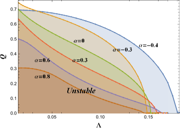
Figure 6: The unstable region of the charged EGB-dS black hole under charged scalar perturbation. The shadows under constant $\alpha$ lines are corresponding unstable regions. We fix $q=1$ here.

Finally, we show the unstable region of the charged EGB-dS black hole under charged scalar perturbation in Fig. 6. The black hole is unstable only when $\Lambda$ and $Q$ are not too large. As $\Lambda$ or $Q$ increase, the black hole becomes less unstable. For positive $\alpha$, the unstable region shrinks. For negative $\alpha$, the unstable region enlarges. Although we do not show the results when $\Lambda\to 0$ due to the limitation of our numerical method, we can expect that there should be sudden drops since we have found that there is no instability for asymptotic flat charged EGB black hole under charged scalar perturbation [11]. This phenomenon was also disclosed for the RN-dS black hole in [24].

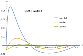
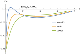
Figure 7: The effective potential when $l=0$. They correspond to the orange line in the upper right panel and orange line in the lower right panel of Fig 4, respectively.

Now let us take a look at the effective potential when $l=0$. In the left panel of Fig. 7, we see that there is a negative potential well between $r_{+}$ and $r_{c}$. This potential well is the key point for the occurrence of instability. However, the negative effective potential does not guarantee $\omega_{I}>0$. For example, the case with $\alpha=0.8$ has a negative potential well, but the corresponding $\omega_{I}<0$. Thus the existence of a negative potential well can be view as the necessary but not sufficient condition for the instability [32]. In the right panel of Fig. 7, the potential well disappears for larger $\alpha$. The perturbation wave can be easily absorbed by the black hole and the corresponding background becomes stable under charged scalar perturbations. Note that the positive cosmological constant is crucial here to creating the necessary potential well.

Now we consider the eigenfrequencies of the charged scalar perturbation when $l=1$. We show the fundamental modes in Fig. 8. The left panel shows that there is still $\omega_{R}\propto Q$ for higher $l$. But $\alpha$ changes $\omega_{R}$ little. All the fundamental modes has $\omega_{R}<\frac{qQ}{r_{c}}$ that live beyond the superradiant condition. The left panel is different from that in Fig. 2. Here $\omega_{I}$ increases with $Q$ and $\alpha$ monotonically. Note that all the modes are stable now.

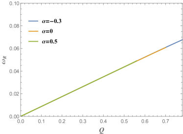
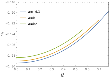
Figure 8: The real part (left) and imaginary part (right) of the fundamental modes when $l=1$. We fix $\Lambda=0.05$ here. The case with other $\Lambda$ are similar.

The stability of the higher $l$ can be explained from the effective potential, as shown in Fig. 9. There is only one potential barrier and not potential well to accumulate the energy to trigger the instability.

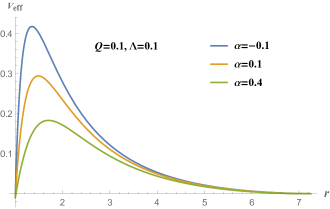
Figure 9: The effective potential when $l=1$. The cases with other $Q,\Lambda$ are similar.

We also provide the detailed time evolution for $l\neq 0$ in Fig. 10. From these two panels we see that the perturbations indeed decays in long time evolution and larger $l$ leads to more significant decay of $\psi$, and hence no instability occurs for higher values of $l$.

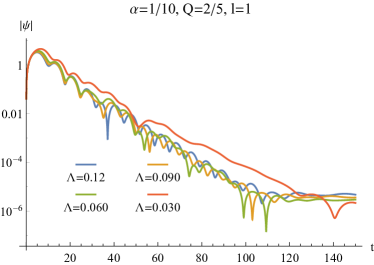
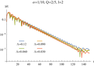
Figure 10: The time evolution of the $|\psi(r_{*}=88.4216,t)|$ in log plot at $\alpha=1/10,\,Q=2/5,\,a=88.4216,\,b=1/10$ and $q=1$, where each curve in both panels corresponds to different values of $\Lambda$. The left and the right panel corresponds to $l=1$ and $l=2$, respectively.

5 Summary and discussion

We studied the instability of charged 4D EGB-dS black hole under the charged massless scalar perturbation. This instability satisfies the superradiant condition. However, not all the modes satisfying the superradiant condition are unstable. The precise mechanism for the this instability is not well understood. But the positive cosmological constant $\Lambda$ should play a crucial role. The instability occurs when the cosmological constant is small. This is reminiscent of the Gregory-Laflamme instability [33] since here exists hierarchy between the black hole event horizon and cosmological horizon. The instability here is different with the “$\Lambda$ instability” found in [12, 21, 22] which occurs when the black hole charge and the cosmological constant are large.

We analyzed this instability from the viewpoint of the effective potential. Higher $l$ has only one potential barrier beyond the event horizon. The perturbation dissipates and leads no instability. The monopole $l=0$ has a negative potential well between the event horizon and cosmological horizon, which can accumulate the energy to trigger the instability. But the negative potential well is just the necessary but not sufficient condition for the instability.

Unlike the cases in asymptotic flat spacetime, the effects of the GB coupling constant $\alpha$ on the perturbation is relevant to the black hole charge and cosmological constant. It makes the unstable black hole more unstable when both the black hole charge and cosmological constant are small, and makes the stable black hole more stable when the black hole charge is large. The weakly charged black hole in dS spacetime is always unstable. The existence of $\alpha$ does not change this phenomenon qualitatively. However, $\alpha$ can change the qualitative behavior when the black hole charge is large, and make the unstable black hole stable. We show that the unstable region of ($\Lambda,Q$) shrinks with positive $\alpha$ can enlarges with negative $\alpha$. Unfortunately, we do not get the accurate enough results when $\Lambda\to 0$ due to the limitation of our numerical method. The case when black hole becomes extremal is also beyond the effectiveness of this method. The stability of extremal black hole may be very different with that of non-extremal black hole. There is “horizon instability” universally [34]. We leave them for further study.

We point out several topics worthy of further investigations. The stability of massive perturbation should be explored in detail to reveal how mass term affects the stability of the charged perturbation. The stability of the 4D charged Einstein-Gauss-Bonnet anti de-Sitter are also definitely interesting to find out. We plan to explore these directions in near future.

6 Acknowledgments

We thanks Peng-Cheng Li, Minyong Guo and Shao-Jun Zhang for helpful discussions. Peng Liu would like to thank Yun-Ha Zha for her kind encouragement during this work. Peng Liu is supported by the Natural Science Foundation of China under Grant No. 11847055, 11905083. Chao Niu is supported by the Natural Science Foundation of China under Grant No. 11805083. C. Y. Zhang is supported by Natural Science Foundation of China under Grant No. 11947067.

References

- [1] D. Lovelock, J.Math.Phys. 12 (1971) 498-501.
- [2] T. Clifton, P. G. Ferreira, A. Padilla and C. Skordis, “Modified Gravity and Cosmology,” Phys. Rept. 513, 1 (2012) [arXiv:1106.2476 [astro-ph.CO]].
- [3] R. P. Woodard, Ostrogradsky’s theorem on Hamiltonian instability, Scholarpedia 10 (2015) no.8, 32243, arXiv:1506.02210 [hep-th]].
- [4] D. J. Gross and J. H. Sloan. The Quartic Effective Action for the Heterotic String. Nucl. Phys., B291:41, 1987.
- [5] D. Glavan and C. Lin, Einstein-Gauss-Bonnet gravity in 4-dimensional space-time, Phys. Rev. Lett. 124, no. 8, 081301 (2020), arXiv:1905.03601 [gr-qc].
- [6] P. G. S. Fernandes, Charged Black Holes in AdS Spaces in 4D Einstein Gauss-Bonnet Gravity, arXiv:2003.05491 [gr-qc].
-
[7]
A. Casalino, A. Colleaux, M. Rinaldi and
S. Vicentini, Regularized Lovelock gravity, arXiv:2003.07068 [gr-qc].
R. A. Konoplya and A. Zhidenko, Black holes in the four-dimensional Einstein-Lovelock gravity, arXiv:2003.07788 [gr-qc].
R. A. Konoplya and A. Zhidenko, BTZ black holes with higher curvature corrections in the 3D Einstein-Lovelock theory, arXiv:2003.12171 [gr-qc].
S. Nojiri and S. D. Odintsov, Novel cosmological and black hole solutions in Einstein and higher-derivative gravity in two dimensions, arXiv:2004.01404 [hep-th].
S.-W. Wei, Y.-X. Liu, Testing the nature of Gauss-Bonnet gravity by four-dimensional rotating black hole shadow, arXiv:2003.07769 [gr-qc].
R. Kumar, S. G. Ghosh, Rotating black holes in the novel 4D Einstein-Gauss-Bonnet gravity, arXiv:2003.08927 [gr-qc].
S. G. Ghosh and S. D. Maharaj, Radiating black holes in the novel 4D Einstein-Gauss-Bonnet gravity, arXiv:2003.09841 [gr-qc].
S. G. Ghosh and R. Kumar, Generating black holes in the novel Einstein-Gauss-Bonnet gravity, arXiv:2003.12291 [gr-qc].
D. V. Singh, S. G. Ghosh and S. D. Maharaj, Clouds of string in novel Einstein-Gauss-Bonnet black holes, arXiv:2003.14136 [gr-qc].
A. Kumar and S. G. Ghosh, Hayward black holes in the novel Einstein-Gauss-Bonnet gravity, arXiv:2004.01131 [gr-qc].
A. Kumar and R. Kumar, Bardeen black holes in the novel Einstein-Gauss-Bonnet gravity, arXiv:2003.13104 [gr-qc].
D. D. Doneva and S. S. Yazadjiev, Relativistic stars in 4D Einstein-Gauss-Bonnet gravity, arXiv:2003.10284 [gr-qc].
W. Y. Ai, A note on the novel 4D Einstein-Gauss-Bonnet gravity, arXiv:2004.02858. -
[8]
T. Kobayashi, Effective scalar-tensor description
of regularized Lovelock gravity in four dimensions, arXiv:2003.12771
[gr-qc].
H. Lu and Y. Pang, Horndeski Gravity as Limit of Gauss-Bonnet, arXiv:2003.11552.
P. G. S. Fernandes, P. Carrilho, T. Clifton, D. J. Mulryne, Derivation of Regularized Field Equations for the Einstein-Gauss-Bonnet Theory in Four Dimensions, arXiv:2004.08362.
Robie A. Hennigar, David Kubiznak, Robert B. Mann, Christopher Pollack, On Taking the limit of Gauss-Bonnet Gravity: Theory and Solutions, arXiv:2004.09472 [gr-qc].
S. Mahapatra, A note on the total action of 4D Gauss-Bonnet theory, arXiv:2004.09214. -
[9]
R. A. Konoplya and A. F. Zinhailo, Quasinormal
modes, stability and shadows of a black hole in the novel 4D Einstein-Gauss-Bonnet
gravity, arXiv:2003.01188 [gr-qc].
R. A. Konoplya and A. Zhidenko, (In)stability of black holes in the 4D Einstein-Gauss-Bonnet and Einstein-Lovelock gravities, arXiv:2003.12492 [gr-qc].
R. A. Konoplya and A. F. Zinhailo, Grey-body factors and Hawking radiation of black holes in 4D Einstein-Gauss-Bonnet gravity, arXiv:2004.02248 [gr-qc].
M. S. Churilova, Quasinormal modes of the Dirac field in the novel 4D Einstein-Gauss-Bonnet gravity, arXiv:2004.00513 [gr-qc].
A. K. Mishra, Quasinormal modes and Strong Cosmic Censorship in the novel 4D Einstein-Gauss-Bonnet gravity, arXiv:2004.01243 [gr-qc].
S. L. Li, P. Wu and H. Yu, Stability of the Einstein Static Universe in 4D Gauss-Bonnet Gravity, arXiv:2004.02080 [gr-qc].
A. Aragón, R. Bécar, P. A. González, Y. Vásquez, Perturbative and nonperturbative quasinormal modes of 4D Einstein-Gauss-Bonnet black holes, arXiv:2004.05632 [gr-qc].
S.-J. Yang, J.-J. Wan, J. Chen, J. Yang, Y.-Q. Wang, Weak cosmic censorship conjecture for the novel 4D charged Einstein-Gauss-Bonnet black hole with test scalar field and particle, arXiv:2004.07934. - [10] C. Y. Zhang, P. C. Li and M. Guo, Greybody factor and power spectra of the Hawking radiation in the novel Einstein-Gauss-Bonnet de-Sitter gravity, arXiv:2003.13068.
- [11] C. Y. Zhang, P. C. Li and M. Guo, Superradiance and stability of the novel 4D charged Einstein-Gauss-Bonnet black hole, arXiv:2004.03141 [gr-qc].
- [12] M.A. Cuyubamba, Stability of asymptotically de Sitter and anti-de Sitter black holes in 4D regularized Einstein-Gauss-Bonnet theory, arXiv:2004.09025 [gr-qc].
-
[13]
M. Guo and P. C. Li, The innermost stable circular
orbit and shadow in the novel Einstein-Gauss-Bonnet gravity,
arXiv:2003.02523 [gr-qc].
M. Heydari-Fard, M. Heydari-Fard and H. R. Sepangi, Bending of light in novel 4D Gauss-Bonnet-de Sitter black holes by Rindler-Ishak method, [arXiv:2004.02140[gr-qc]].
X. h. Jin, Y.-x. Gao and D. j. Liu Strong gravitational lensing of a 4D Einstein-Gauss-Bonnet black hole in homogeneous plasma, [arXiv:2004.02261[gr-qc]].
Y. P. Zhang, S. W. Wei and Y. X. Liu, Spinning test particle in four-dimensional Einstein-Gauss-Bonnet Black Hole, arXiv:2003.10960 [gr-qc].
S. U. Islam, R. Kumar and S. G. Ghosh, Gravitational lensing by black holes in $4D$ Einstein-Gauss-Bonnet gravity, arXiv:2004.01038 [gr-qc].
J. Rayimbaev, A. Abdujabbarov, B. Turimov, F. Atamurotov, Magnetized particle motion around 4-D Einstein-Gauss-Bonnet Black Hole, arXiv:2004.10031 [gr-qc]. -
[14]
K. Hegde, A. N. Kumara, C. L. A. Rizwan, A.
K. M. and M. S. Ali, Thermodynamics, Phase Transition and Joule Thomson
Expansion of novel 4-D Gauss Bonnet AdS Black Hole, arXiv:2003.08778
[gr-qc].
S. W. Wei and Y. X. Liu, Extended thermodynamics and microstructures of four-dimensional charged Gauss-Bonnet black hole in AdS space, arXiv:2003.14275 [gr-qc].
D. V. Singh and S. Siwach, Thermodynamics and P-v criticality of Bardeen-AdS Black Hole in 4-D Einstein-Gauss-Bonnet Gravity, arXiv:2003.11754 [gr-qc].
S. A. Hosseini Mansoori, Thermodynamic geometry of novel 4-D Gauss Bonnet AdS Black Hole, arXiv:2003.13382 [gr-qc].
B. Eslam Panah, Kh. Jafarzade, 4D Einstein-Gauss-Bonnet AdS Black Holes as Heat Engine, arXiv:2004.04058 [hep-th].
S. Ying, Thermodynamics and Weak Cosmic Censorship Conjecture of 4D Gauss-Bonnet-Maxwell Black Holes via Charged Particle Absorption, arXiv:2004.09480 [gr-qc] - [15] D. Malafarina, B. Toshmatov, N. Dadhich, Dust collapse in 4D Einstein-Gauss-Bonnet gravity, arXiv:2004.07089 [gr-qc].
-
[16]
C. Liu, T. Zhu and Q. Wu, Thin Accretion Disk
around a four-dimensional Einstein-Gauss-Bonnet Black Hole, arXiv:2004.01662
[gr-qc].
A. Naveena Kumara, C.L. Ahmed Rizwan, K. Hegde, Md Sabir Ali, Ajith K.M, Rotating 4D Gauss-Bonnet black hole as particle accelerator, arXiv:2004.04521 [gr-qc].
F.-W. Shu, Vacua in novel 4D Eisntein-Gauss-Bonnet Gravity: pathology and instability, arXiv:2004.09339 [gr-qc]. -
[17]
R. A. Konoplya, A. Zhidenko, Quasinormal modes
of black holes: From astrophysics to string theory, Rev.Mod.Phys.
83 (2011) 793-836, arXiv:1102.4014 [gr-qc].
E. Berti, V. Cardoso, A. O. Starinets, Quasinormal modes of black holes and black branes, Class.Quant.Grav. 26 (2009) 163001, arXiv:0905.2975 [gr-qc]. - [18] C. Y. Zhang, S. J. Zhang, and B. Wang, Superradiant instability of Kerr-de Sitter black holes in scalar-tensor theory, J. High Energy Phys. 08 (2014) 011. arXiv:1405.3811.
-
[19]
V. Cardoso, J. a. L. Costa, K. Destounis, P.
Hintz, and A. Jansen, Quasinormal modes and Strong Cosmic Censorship,
Phys. Rev. Lett. 120 (2018) no. 3, 031103, arXiv:1711.10502.
Y. Mo, Y. Tian, B. Wang, H. Zhang, Z. Zhong, Strong cosmic censorship for the massless charged scalar field in the Reissner-Nordstrom-de Sitter spacetime, Phys. Rev. D 98, 124025 (2018), arXiv:1808.03635 [gr-qc].
H. Liu, Z. Tang, K. Destounis, B. Wang, E. Papantonopoulos, H. Zhang, Strong Cosmic Censorship in higher-dimensional Reissner-Nordström-de Sitter spacetime, JHEP 03 (2019) 187, arXiv:1902.01865 [gr-qc]. - [20] H. Zhang, Z. Zhong, Strong cosmic censorship in de Sitter space: As strong as ever, arXiv:1910.01610 [hep-th].
-
[21]
R. A. Konoplya and A. Zhidenko, Instability
of higher dimensional charged black holes in the de-Sitter world,
Phys. Rev. Lett. 103 (2009) 161101, arXiv:0809.2822 [hep-th].
R. A. Konoplya and A. Zhidenko, Instability of D-dimensional extremally charged ReissnerNordstrom(-de Sitter) black holes: Extrapolation to arbitrary D, Phys. Rev. D 89, no. 2, 024011 (2014) [arXiv:1309.7667 [hep-th]].
M. A. Cuyubamba, R. A. Konoplya and A. Zhidenko, Quasinormal modes and a new instability of Einstein-Gauss-Bonnet black holes in the de Sitter world, Phys.Rev. D 93 (2016) no.10, 104053, arXiv:1604.03604 [gr-qc]. -
[22]
P.-C. Li, C.-Y. Zhang, B. Chen, The Fate of Instability
of de Sitter Black Holes at Large D, JHEP 1911 (2019) 042, arXiv:1909.02685
[hep-th].
C. Y. Zhang, S. J. Zhang, D. C. Zou, B. Wang, Charged scalar gravitational collapse in de Sitter spacetime, Phys.Rev. D93 (2016) no.6, 064036, arXiv:1512.06472 [gr-qc]. - [23] Z. Zhu, S.-J. Zhang, C. E. Pellicer, B. Wang, Elcio Abdalla, Stability of Reissner-Nordström black hole in de Sitter background under charged scalar perturbation, Phys.Rev. D90 (2014) no.4, 044042, Addendum: Phys.Rev. D90 (2014) no.4, 049904, arXiv:1405.4931 [hep-th].
- [24] R. A. Konoplya, A. Zhidenko, Charged scalar field instability between the event and cosmological horizons, Phys. Rev. D 90, 064048 (2014), arXiv:1406.0019 [hep-th].
- [25] K. Destounis, Superradiant instability of charged scalar fields in higher-dimensional Reissner Nordstrom de Sitter black holes, Phys. Rev. D100 (2019) no. 4, 044054, arXiv:1908.06117 [gr-qc].
- [26] R. Brito, V. Cardoso, P. Pani, Superradiance – the 2020 Edition, Lect.Notes Phys. 906 (2015) pp.1-237, arXiv:1501.06570 [gr-qc].
-
[27]
R. G. Cai, L. M. Cao and N. Ohta, “Black Holes
in Gravity with Conformal Anomaly and Logarithmic Term in Black Hole
Entropy,” JHEP 1004, 082 (2010), arXiv:0911.4379.
Y. Tomozawa, “Quantum corrections to gravity,” arXiv:1107.1424 [gr-qc].
G. Cognola, R. Myrzakulov, L. Sebastiani and S. Zerbini, “Einstein gravity with GaussBonnet entropic corrections,” Phys. Rev. D 88, no. 2, 024006 (2013), arXiv:1304.1878. -
[28]
C.-Y. Zhang, P.-C. Li, B. Chen, Greybody factors
for Spherically Symmetric Einstein-Gauss-Bonnet-de Sitter black hole,
Phys.Rev. D97 (2018) no.4, 044013, arXiv:1712.00620.
P.-C. Li, C.-Y. Zhang, Hawking radiation for scalar fields by Einstein-Gauss-Bonnet-de Sitter black holes, Phys.Rev. D99 (2019) no.2, 024030, arXiv:1901.05749 [hep-th]. - [29] C. Y. Zhang, S. J. Zhang, and B. Wang, Charged scalar perturbations around Garfinkle–Horowitz–Strominger black holes, Nucl. Phys. B899, 37 (2015). arXiv:1501.03260.
-
[30]
R. L. H. H. Ciftci and N. Saad. Asymptotic iteration
method for eigenvalue problems, Journal of Physics A, 2003, vol.36,
no. 47: 11807–11816, arXiv:math-ph/0309066.
R. L. H. H. Ciftci and N. Saad. Perturbation theory in a framework of iteration methods, Physics Letters A, 2005, vol. 340, no. 5-6: 388–396, arXiv:math-ph/0504056. -
[31]
H. T. Cho, A. S. Cornell, J. Doukas, W. Naylor,
Black hole quasinormal modes using the asymptotic iteration method.
Class. Quant. Grav. 2010, 27: 155004, arXiv:0912.2740.
H. T. Cho, A. S. Cornell, J. Doukas, T. R. Huang, W. Naylor, A New Approach to Black Hole Quasinormal Modes: A Review of the Asymptotic Iteration Method. Adv. Math. Phys. 2012, 2012: 281705, arXiv:1111.5024 [gr-qc]. - [32] K. A. Bronnikov, R. A. Konoplya and A. Zhidenko, Instabilities of wormholes and regular black holes supported by a phantom scalar field, Phys. Rev. D 86, 024028 (2012) [arXiv:1205.2224].
-
[33]
R. Gregory and R. Laflamme, Black strings and
p-branes are unstable, Phys.Rev.Lett. 70 (1993) 2837-2840, arXiv:hep-th/9301052
[hep-th].
R.Gregory, R.Laflamme, Black Strings and p-Branes are Unstable, Phys.Rev.Lett.70:2837-2840,1993, arXiv:hep-th/9301052. -
[34]
S. Aretakis, Decay of Axisymmetric Solutions of the Wave Equation on Extreme Kerr Backgrounds, J. Funct. Anal. 263, 2770 (2012) [arXiv:1110.2006 [gr-qc]]
S. Aretakis, Horizon Instability of Extremal Black Holes, Adv.Theor.Math.Phys. 19 (2015) 507-530, arXiv:1206.6598 [gr-qc]
S.-J. Zhang, Q. Pan, B. Wang, Elcio Abdalla, Horizon instability of massless scalar perturbations of an extreme Reissner-Nordström-AdS black hole, JHEP 1309 (2013) 101, arXiv:1308.0635 [hep-th].