The role of Coherent Structures and Inhomogeneity in Near-Field Inter-Scale Turbulent Energy Transfers

Abstract

We use Direct Numerical Simulation (DNS) data to study inter-scale and inter-space energy exchanges in the near-field of a turbulent wake of a square prism in terms of a Kármán-Howarth-Monin-Hill (KHMH) equation written for a triple decomposition of the velocity field which takes into account the presence of quasi-periodic vortex shedding coherent structures. Concentrating attention on the plane of the mean flow and on the geometric centreline, we calculate orientation-averages of every term in the KHMH equation. The near-field considered here ranges between 2 and 8 times the width $d$ of the square prism and is very inhomogeneous and out of equilibrium so that non-stationarity and inhomogeneity contributions to the KHMH balance are dominant. The mean flow produces kinetic energy which feeds the vortex shedding coherent structures. In turn, these coherent structures transfer their energy to the stochastic turbulent fluctuations over all length-scales $r$ from the Taylor length $\lambda$ to $d$ and dominate spatial turbulent transport of small-scale two-point stochastic turbulent fluctuations. The orientation-averaged non-linear inter-scale transfer rate $\Pi^{a}$ which was found to be approximately independent of $r$ by Alves Portela et al. (2017) in the range $\lambda\leq r\leq 0.3d$ at a distance $x_{1}=2d$ from the square prism requires an inter-scale transfer contribution of coherent structures for this approximate constancy. However, the near-constancy of $\Pi^{a}$ in the range $\lambda\leq r\leq d$ at $x_{1}=8d$ which was also found by Alves Portela et al. (2017) is mostly attributable to stochastic fluctuations. Even so, the proximity of $-\Pi^{a}$ to the turbulence dissipation rate $\varepsilon$ in the range $\lambda\leq r\leq d$ at $x_{1}=8d$ does require inter-scale transfer contributions of the coherent structures. Spatial inhomogeneity also makes a direct and distinct contribution to $\Pi^{a}$, and the constancy of $-\Pi^{a}/\varepsilon$ close to $1$ would not have been possible without it either in this near-field flow. Finally, the pressure-velocity term is also an important contributor to the KHMH balance in this near-field, particularly at scales $r$ larger than about $0.4d$, and appears to correlate with the purely stochastic non-linear inter-scale transfer rate when the orientation average is lifted.

1 Introduction

Coherent flow structures are present in most turbulent flows. Coherent structures associated with vortex shedding, in particular, are clearly present in turbulent wakes. One can expect these structures to have some impact on a two-point energy balance which takes into account both inter-scale and inter-space energy transfers. Such an energy balance which can be applied to turbulent flows which are not necessarily homogeneous and isotropic has already been used by various authors to analyse turbulent flows starting with Marati et al. (2004) who applied it to turbulent channel flow. This energy balance, first derived by Hill (2002b) (but see also Duchon & Robert (2000)), is sometimes referred to as the Kármán-Howarth-Monin-Hill (KHMH) equation because it fully generalises the Kármán-Howarth-Monin equation (see Frisch (1995)) which is limited to homogeneous and to periodic turbulence. To our knowledge, there has been, to date, only one study of such an energy balance in a boundary free turbulent shear flow which takes account of coherent structures. This is the study of Thiesset et al. (2014) who derived a KHMH equation written for a triple decomposition, where the coherent quasi-periodic part of the fluctuating velocity field is explicitly treated in the analysis as distinct from the stochastic turbulent fluctuations. Thiesset et al. (2014) applied their two-point equation to a turbulent wake of a cylinder and concentrated attention at downstream distances between $10d$ and $40d$, where $d$ is the diameter of the cylinder. They found that the coherent structures impose a forcing on the stochastic fluctuations and proposed an analytical model which describes the energy content of such structures in scale space.

The one other study of the KHMH equation in a planar turbulent wake is that of Alves Portela et al. (2017) who looked at inter-scale and inter-space exchanges in the near wake of a square prism of side width $d$ but did not consider the effects of vortex shedding coherent structures. They found that $\Pi^{a}$, the rate at which turbulent energy is transferred across scales when averaged over orientations in the plane of the mean-flow (plane normal to coordinate $x_{3}$), is roughly constant, and in fact close to the turbulence dissipation rate $\varepsilon$, over a wide range of scales at a distance $8d$ from the square prism. Their Direct Numerical Simulation (DNS) showed that this is also true, albeit over a much reduced range of length-scales, at a distance $2d$ from the square prism. Their KHMH analysis made it clear that this Kolmogorov-sounding constancy of $\Pi^{a}$ cannot be the result of a Kolmogorov equilibrium cascade given that the near-field region of the flow where it is observed is very inhomogeneous, anisotropic and out of equilibrium. One is therefore naturally faced with the question of the role of the coherent structures in establishing $-\Pi^{a}/\varepsilon\approx 1$ and the extent in which this approximate constancy is due to the stochastic component of the turbulent fluctuations. We also attempt to address the direct contribution of spatial inhomogeneity to the behaviour of $\Pi^{a}$.

In this paper we use the triple decomposition KHMH equations of Thiesset et al. (2014) which we slightly generalise to include mean flow velocity differences. We analyse the data obtained by Alves Portela et al. (2017) from their DNS of the turbulent planar wake of a square prism of side length $d$. The inlet free-stream velocity $U_{\infty}$ in this DNS is such that $U_{\infty}d/\nu=3900$ where $\nu$ is the fluid’s kinematic viscosity. We refer to Alves Portela et al. (2017) for details of this DNS.

In § 2 we explain how the triple decomposition is carried out and how we extract from the time-varying fields of velocity and pressure a contribution associated with the vortex shedding. In § 3 we detail the scale-by-scale KHMH budgets that we use in this paper to explore combined inter-scale and inter-space transfers in the near wake of a square prism and in § 4 we report on the various terms in our KHMH budgets in an orientation-averaged sense. § 5 presents our results on inter-scale energy transfers and scale-space fluxes and we conclude in § 6.

2 Triply Decomposed Velocity Field

The Reynolds decomposition distinguishes between the mean field and the fluctuating field. When the flow exhibits a well-defined non-stochastic (e.g. periodic) flow feature, one can further decompose the fluctuating field into a coherent field and a stochastic field (Reynolds & Hussain, 1972; Hussain & Reynolds, 1970). The velocity field is therefore the sum of three fields: ${\bf{u}_{full}}=\bf{U}+\tilde{\bf{u}}+\bf{u}^{\prime}$ where $\bf{U}$ is the mean velocity field obtained by time-averaging ${\bf{u}_{full}}$, and where $\tilde{\bf{u}}$ and $\bf{u}^{\prime}$ are the coherent and stochastic parts, respectively, of the fluctuating velocity field. The coherent fluctuating velocity $\tilde{\bf{u}}$ is obtained by phase-averaging ${\bf{u}_{full}}-\bf{U}$ and the stochastic fluctuating velocity is the remainder and is obtained from $\bf{u}^{\prime}={\bf{u}_{full}}-\bf{U}-\tilde{\bf{u}}$. If ${\bf{u}_{full}}$ is incompressible, $\bf{U}$, $\tilde{\bf{u}}$ and $\bf{u}^{\prime}$ are incompressible too. With similar notation one also decomposes the pressure field: $p=P+\tilde{p}+p^{\prime}$. In the present work which is concerned with the planar wake of a square prism, both time- and phase-averaging operations also involve averaging in the span-wise direction, i.e. in the direction $x_{3}$ which is normal to the plane of the average wake flow. Fluid velocities and spatial coordinates in the stream-wise direction are denoted by $U_{1}$, $\tilde{u}_{1}$, $u^{\prime}_{1}$, and $x_{1}$ respectively; in the cross-stream direction they are $U_{2}$, $\tilde{u}_{2}$, $u^{\prime}_{2}$, and $x_{2}$. The span-wise fluid velocity components are $U_{3}$, $\tilde{u}_{3}$, $u^{\prime}_{3}$.

The definitions of $\tilde{\bf{u}}$ and $\tilde{p}$ require a reference phase. One can obtain a reference phase from a pressure tap on the cylinder (see e.g. Braza et al., 2006) or from the fluctuating velocity signal, either from within the turbulent flow after appropriately filtering (see e.g. Thiesset et al., 2014) or from the outside of the turbulent core (see e.g. Davies, 1976). Wlezien & Way (1979) provide an extensive comparison of different methods with focus on experimental techniques.

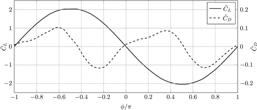
In the present analysis, the phase angle $\phi$ used to compute phase-averages is extracted from the Hilbert transform of the lift coefficient $C_{L}$ (see Feldman, 2011, for details on the Hilbert transform). This choice follows naturally from the fact that the lift on the square prism in our flow closely follows a sinusoid in time.

The data being discrete in time, $\phi$ was binned into $32$ groups. A smaller bin size would have improved phase-resolution but would have reduced statistical convergence (as fewer samples would have fallen within each bin). Thus, each time instant is associated with a value $\phi=-\pi+n\frac{2\pi}{32}$ where $0<n<31$. The resulting phase-averaged lift and drag coefficients are plotted in fig. 1 versus the phase angle $\phi$, where $\phi=0$ has been chosen such that $\tilde{C}_{L}(\phi=0)=0$.

Figure 1: Evolution of phase-averaged lift and drag coefficients $\tilde{C}_{L}$ and $\tilde{C}_{D}$ along the normalised phase $\phi/\pi$.

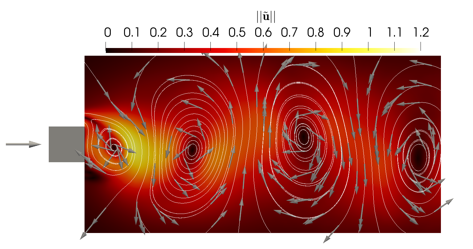
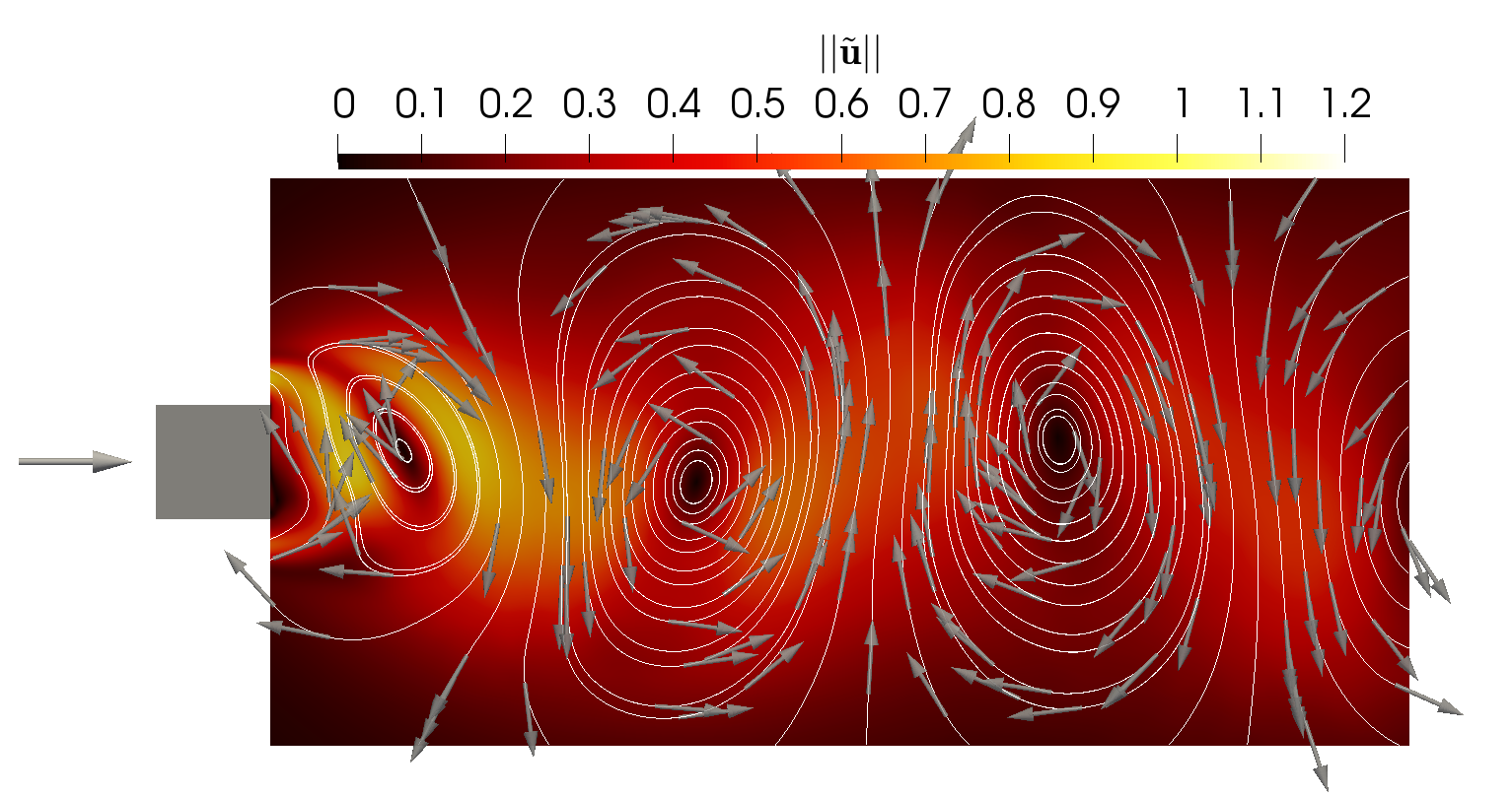
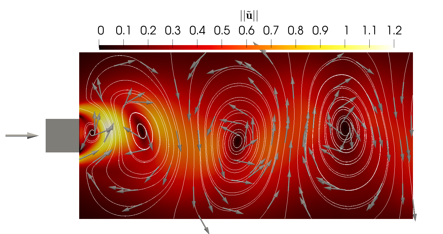
The phase-averaged velocity field $\tilde{\mathbf{u}}$ is shown in fig. 2 for four different values of $\phi$: $0$, $\frac{1}{4}\pi$, $\frac{1}{2}\pi$ and $\frac{3}{4}\pi$.

It clearly displays a structure similar to that of the von Kármán vortex street where the alternating vortices display opposite circulation, the positive ones travelling slightly above and the negative ones slightly below the centreline. Note that $\tilde{u}_{3}=0$ uniformly and that $\tilde{u}_{1}$ and $\tilde{u}_{2}$ depend on $x_{1}$ and $x_{2}$ but not on $x_{3}$.

Figure 2: Contours of the magnitude of the phase-averaged velocity $\tilde{\mathbf{u}}$ (normalised by $U_{\infty}$), and white unit vectors locally parallel to $\tilde{\mathbf{u}}$. The large arrow on the left indicates the direction of the free-stream velocity $U_{\infty}$. Using the phase angles shown in fig. 1, on the top row $\phi=0$ (left) and $\phi=\frac{1}{4}\pi$ (right); on the bottom row $\phi=\frac{1}{2}\pi$ (left) and $\phi=\frac{3}{4}\pi$ (right).

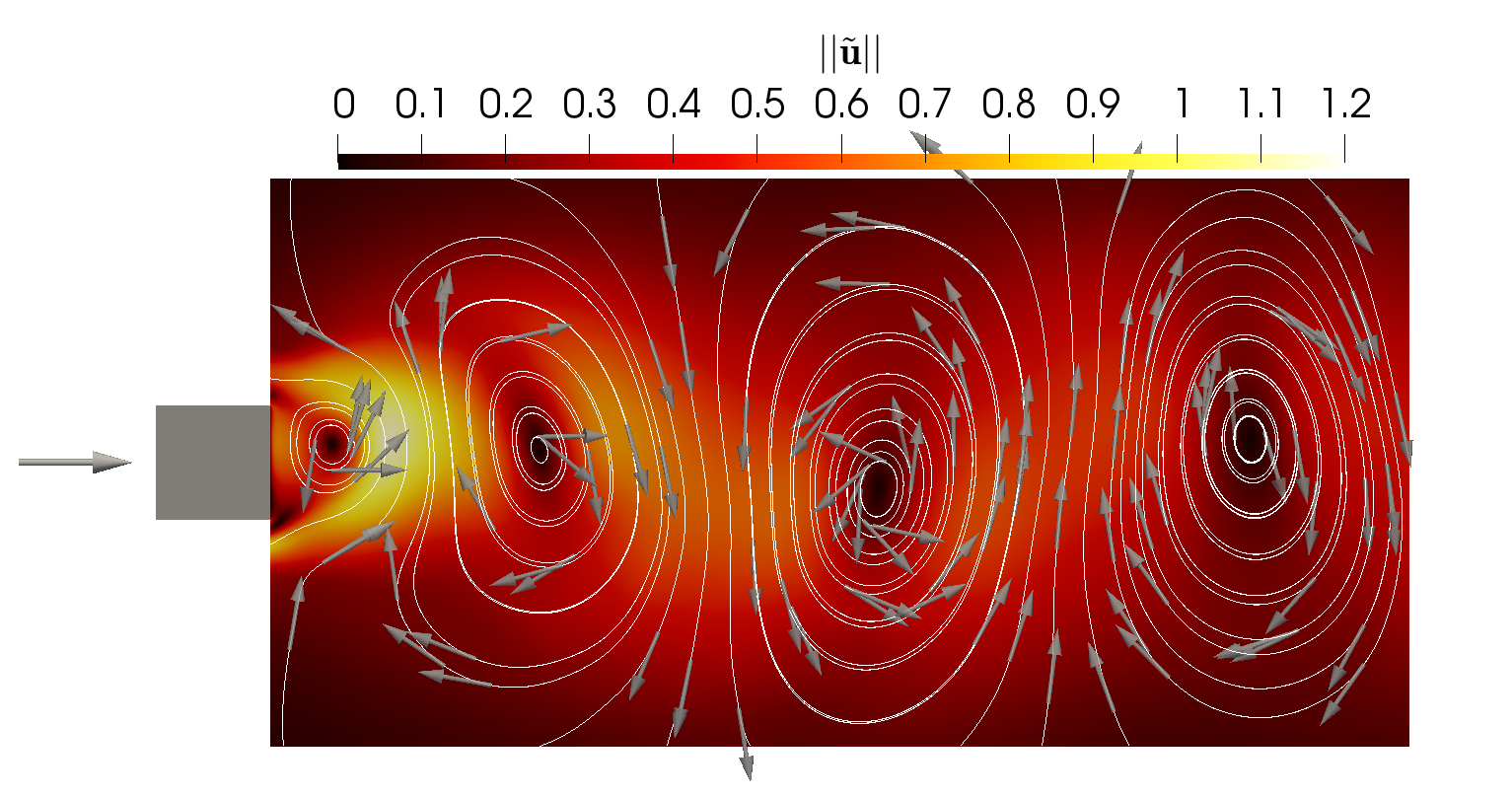
The coherent vorticity field ${\bf\nabla}\times\tilde{\bf{u}}$ is aligned with the span-wise direction and therefore has only one non-zero component $\tilde{\omega}_{3}$. As shown in Alves Portela et al. (2018) for this exact same flow (see their fig. 3), lines of constant vorticity approximately coincide with streamlines of $\tilde{\bf{u}}$. As discussed in Hussain (1983), the streamlines are not necessarily good indicators of the presence of coherent structures, but Lyn et al. (1995) argue that, apart from the base region in the very near wake where the coherent structures are formed, there is indeed a correspondence between iso-vorticity and streamlines in identifying coherent structures.

The spectra of the full fluctuating velocity component $\tilde{u}_{1}+u^{\prime}_{1}$ and $\tilde{u}_{2}+u^{\prime}_{2}$ are compared to those of their stochastic counterparts $u^{\prime}_{1}$ and $u^{\prime}_{2}$ in fig. 3. As is well known, the shedding frequency is double in the spectrum of $\tilde{u}_{1}+u^{\prime}_{1}$ compared to the spectrum of $\tilde{u}_{2}+u^{\prime}_{2}$, and we checked that it corresponds to the distance between coherent vortices in fig. 2 (the distance between successive such vortices does not vary much). Note that the energetic peak present at the shedding frequency in the spectrum of $\tilde{u}_{1}+u^{\prime}_{1}$ is absent in the spectrum of $u^{\prime}_{1}$ and that the energetic peak present at the shedding frequency in the spectrum of $\tilde{u}_{2}+u^{\prime}_{2}$ is absent in the spectrum of $u^{\prime}_{2}$.

Figure 3: Power spectrum densities normalised by $U_{\infty}d$ of stream-wise (left) and cross-stream (right) fluctuating velocities, before (dashed lines) and after (full lines) removing the phase component, between $x_{1}/d=1$ (blue/top) and $x_{1}/d=8$ (dark green/bottom) offset by one decade every $d$. The dashed line indicates a slope of $-5/3$ and the dotted line indicates $f=2f_{s}$ (left) and $f=f_{s}$ (right).

Figure 4: Profiles of kinetic energies $\tilde{k}$ and $k^{\prime}$ computed from the phase and stochastic components, respectively, along the centreline. The total kinetic energy $k=\tilde{k}+k^{\prime}$ is also shown for comparison.

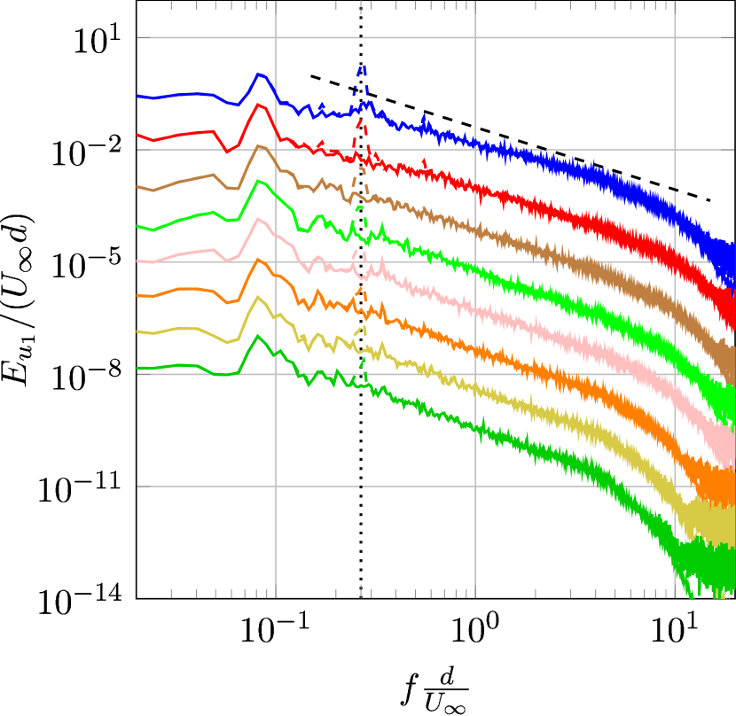
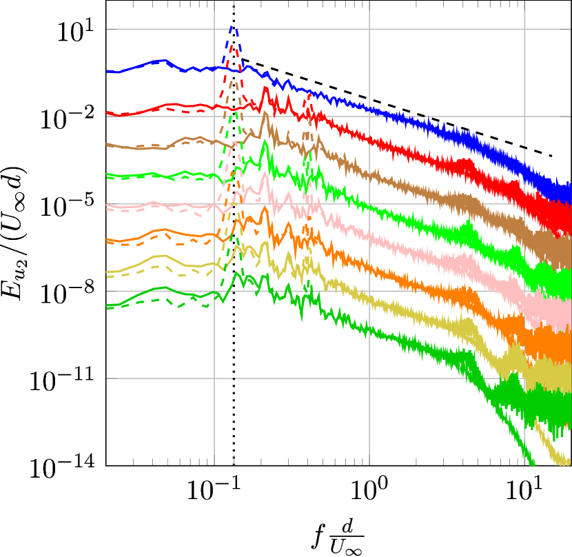
In conclusion, the phase-averaged fluctuating velocity $\tilde{\mathbf{u}}$ is representative of the coherent structures in the present flow as it contains the shedding’s characteristic time signature, and its spatial distribution (fig. 2) is one of approximately periodic large scale vortices.

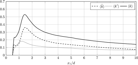
In Hussain (1983); Hussain et al. (1987) it is argued that these coherent structures do not necessarily provide a large contribution to the turbulent kinetic energy. Of course, the regions of the flow considered by these authors are much further downstream than the region of the flow studied here. Figure 4 makes it clear that the coherent structures contribute most of the turbulent kinetic energy $k\equiv{1\over 2}\langle|\tilde{\mathbf{u}}+\mathbf{u}^{\prime}|^{2}\rangle$ in the near wake considered here and that their contribution ($\tilde{k}\equiv{1\over 2}\langle|\tilde{\mathbf{u}}|^{2}\rangle$) decreases, in the direction of the mean flow, at a faster rate than the kinetic energy associated with the stochastic motions ($k^{\prime}\equiv{1\over 2}\langle|\mathbf{u}^{\prime}|^{2}\rangle$) in-line with Hussain (1983); Hussain et al. (1987). (The brackets $\langle...\rangle$ symbolise combined time- and span-wise-average operations using approximately $10^{3}$ snapshots spanning just over $32$ shedding cycles. The additional span-wise average involves $150$ planes in the span-wise direction which is statistically homogeneous. This level of statistics proved sufficient to converge the averages of all the quantities presented in this paper.) Note that $k=\tilde{k}+k^{\prime}$. Note also that the Taylor length-based Reynolds number $Re_{\lambda}$ varies on the centreline from about 120 at $x_{1}/d=2$ to about 170 at $x_{1}/d=10$ if it is defined on the basis of $\sqrt{\langle{u^{\prime}_{1}}^{2}\rangle}$ and from about 100 at $x_{1}/d=2$ to about 190 at $x_{1}/d=10$ if it is defined on the basis of $\sqrt{2k^{\prime}/3}$.

In the following section we introduce scale-by-scale energy budgets adapted to the triple decomposition of a velocity field into its mean and its coherent and stochastic fluctuations.

3 Scale-by-scale Energy Budgets

The most general forms of scale-by-scale energy budget have been derived by Hill (1997, 2001, 2002a) and Duchon & Robert (2000) without making any assumption on the nature of the turbulence. Using the Reynolds decomposition and averaging over time in general but also in the span-wise direction for this paper’s particular flow, this equation (which we refer to as Kármán-Howarth-Monin-Hill (KHMH) equation) follows from the Navier-Stokes equation and incompressibility and takes the form

$$\frac{U_{i}^{+}+U_{i}^{-}}{2}{\frac{\partial\langle\delta q^{2}\rangle}{\partial x_{i}}}+{\frac{\partial\langle\delta u_{i}\delta q^{2}\rangle}{\partial r_{i}}}+{\frac{\partial\delta U_{i}\langle\delta q^{2}\rangle}{\partial r_{i}}}=-2\langle{\delta u_{i}\delta u_{j}}\rangle\frac{\partial\delta U_{j}}{\partial r_{i}}-\\ -\langle{\left(u_{i}^{+}+u_{i}^{-}\right)\delta u_{j}}\rangle\frac{\partial\delta U_{j}}{\partial x_{i}}-{\frac{\partial\langle\frac{u_{i}^{+}+u_{i}^{-}}{2}\delta q^{2}\rangle}{\partial x_{i}}}-2\frac{\partial\langle{\delta u_{i}\delta p\rangle}}{\partial x_{i}}+\nu\frac{1}{2}\frac{\partial^{2}\langle{\delta q^{2}}\rangle}{\partial x_{i}\partial x_{i}}+\\ +2\nu\frac{\partial^{2}\langle{\delta q^{2}}\rangle}{\partial r_{i}\partial r_{i}}-4\nu\left(\langle{\frac{\partial\delta u_{j}}{\partial x_{i}}\frac{\partial\delta u_{j}}{\partial x_{i}}}\rangle+\frac{1}{4}\langle{\frac{\partial\delta u_{j}}{\partial r_{i}}\frac{\partial\delta u_{j}}{\partial r_{i}}}\rangle\right)$$ (1)

where $\delta q^{2}\equiv\delta u_{i}\delta u_{i}$ in terms of the fluctuating velocity differences $\delta u_{i}\equiv(\tilde{u}_{i}^{+}+{u^{\prime}_{i}}^{+})-(\tilde{u}_{i}^{-}+{u^{\prime}_{i}}^{-})$ (for components $i=1,2,3$), $\delta U_{i}\equiv U_{i}^{+}-U_{i}^{-}$, $\delta p\equiv(\tilde{p}^{+}+p^{\prime+})-(\tilde{p}^{-}+p^{\prime-})$, and the superscripts $+$ and $-$ distinguish quantities evaluated at positions ${\bf\xi}^{+}\equiv{\bf x}+{\bf r}/2$ and ${\bf\xi}^{-}\equiv{\bf x}-{\bf r}/2$, respectively; e.g. $u^{+}_{i}\equiv\tilde{u}_{i}^{+}+{u^{\prime}_{i}}^{+}$ and $u^{-}_{i}\equiv\tilde{u}_{i}^{-}+{u^{\prime}_{i}}^{-}$ are the full fluctuating velocity components at ${{\bf\xi}^{+}}$ and ${{\bf\xi}^{-}}$ respectively. Equation (1) is written in a six-dimensional reference frame $x_{i},r_{i}$ where coordinates $x_{i}$ of ${\bf x}$ are associated with a location in physical space and the scale space is the space of all separations and orientations ${\bf r}=(r_{1},r_{2},r_{3})$ between two-points (we refer to $r=|{\bf r}|$ as a scale). If the average operation is not over time but over realisations, then the extra term $\frac{\partial\langle\delta q^{2}\rangle}{\partial t}$ can also be present on the left hand side of equation (1). (Note that an even more general form of the KHMH equation can be obtained without any decomposition and without any averaging operation, see Duchon & Robert (2000), Hill (2002a) and Yasuda & Vassilicos (2018).)

Following Valente & Vassilicos (2015); Gomes-Fernandes et al. (2015); Alves Portela et al. (2017), each term in (1), re-written as

$$\mathcal{A}+\Pi+\Pi_{U}=\mathcal{P}+\mathcal{T}_{u}+\mathcal{T}_{p}+\mathcal{D}_{x}+\mathcal{D}_{r}-\varepsilon_{r},$$ (2)

is associated with a physical process in the budget of $\langle\delta q^{2}\rangle$ as follows:

• $4\mathcal{A}=\frac{U_{i}^{+}+U_{i}^{-}}{2}{\frac{\partial\langle\delta q^{2}\rangle}{\partial x_{i}}}$ is the mean advection term.

• $4\Pi=\frac{\partial\langle\delta u_{i}\delta q^{2}\rangle}{\partial r_{i}}$ is the non-linear inter-scale transfer rate which accounts for the effect of non-linear interactions in redistributing $\delta q^{2}$ within the $r_{i}$ space and is given by the divergence in scale space of the flux $\langle\delta u_{i}\delta q^{2}\rangle$.

• $4\Pi_{U}=\frac{\partial\delta U_{i}\langle\delta q^{2}\rangle}{\partial r_{i}}$ is the linear inter-scale transfer rate. (The term “linear” used here does not mean that a linearisation of the Navier-Stokes equation has been performed.)

• $4\mathcal{P}=-2\langle{\delta u_{i}\delta u_{j}}\rangle\frac{\partial\delta U_{j}}{\partial r_{i}}-\langle{\left(u_{i}^{+}+u_{i}^{-}\right)\delta u_{j}}\rangle\frac{\partial\delta U_{j}}{\partial x_{i}}$ can be associated with the production of $\langle\delta q^{2}\rangle$ by mean flow gradients. (See Alves Portela et al. (2017) for more details.)

• $4\mathcal{T}_{u}=-\frac{\partial\langle\frac{u_{i}^{+}+u_{i}^{-}}{2}\delta q^{2}\rangle}{\partial x_{i}}$ is the transport of $\delta q^{2}$ in physical space due to turbulent fluctuations.

• $4\mathcal{T}_{p}=-2\frac{\partial\langle{\delta u_{i}\delta p\rangle}}{\partial x_{i}}$ is the pressure-velocity term, equal to $-2$ times the correlation between fluctuating velocity differences and differences of fluctuating pressure gradient.

• $4\mathcal{D}_{x}=\nu\frac{1}{2}\frac{\partial^{2}\langle{\delta q^{2}}\rangle}{\partial x_{i}\partial x_{i}}$ is the viscous diffusion in physical space.

• $4\mathcal{D}_{r}=2\nu\frac{\partial^{2}\langle{\delta q^{2}}\rangle}{\partial r_{i}\partial r_{i}}$ is the viscous diffusion in scale space. This term is equal to the dissipation $\varepsilon$ when the two points coincide ($r=0$) and can be shown (see Appendix B in Valente & Vassilicos, 2015) to be negligible for separations larger than the Taylor micro-scale.

• $4\varepsilon_{r}=4\nu\left(\langle{\frac{\partial\delta u_{j}}{\partial x_{i}}\frac{\partial\delta u_{j}}{\partial x_{i}}}\rangle+\frac{1}{4}\langle{\frac{\partial\delta u_{j}}{\partial r_{i}}\frac{\partial\delta u_{j}}{\partial r_{i}}}\rangle\right)$ and $\varepsilon_{r}$ is actually the two-point average dissipation rate $\varepsilon_{r}=\frac{\varepsilon^{+}+\varepsilon^{-}}{2}$ as it equals $\frac{1}{2}\nu\left(\langle{\frac{\partial u_{j}^{+}}{\partial x_{i}^{+}}\frac{\partial u_{j}^{+}}{\partial x_{i}^{+}}}\rangle+\langle{\frac{\partial u_{j}^{-}}{\partial x_{i}^{-}}\frac{\partial u_{j}^{-}}{\partial x_{i}^{-}}}\rangle\right)$.

With the triple decomposition introduced in § 2 one can decompose the second order structure function $\langle\delta{q}^{2}\rangle$ into a stochastic and coherent part, i.e. $\langle\delta{q}^{2}\rangle=\langle\delta\tilde{q}^{2}\rangle+\langle\delta{q^{\prime}}^{2}\rangle$ where $\delta\tilde{q}^{2}\equiv\delta\tilde{u}_{i}\delta\tilde{u}_{i}$ with $\delta\tilde{u}_{i}\equiv\tilde{u}_{i}^{+}-\tilde{u}_{i}^{-}$ and $\delta{q^{\prime}}^{2}\equiv\delta u^{\prime}_{i}\delta u^{\prime}_{i}$ with $\delta u^{\prime}_{i}\equiv{u^{\prime}_{i}}^{+}-{u^{\prime}_{i}}^{-}$. The fluctuating pressure difference $\delta p$ is also decomposed in a similar way, i.e. $\delta p=\delta\tilde{p}+\delta p^{\prime}$ where $\delta\tilde{p}\equiv\tilde{p}^{+}-\tilde{p}^{-}$ and $\delta p^{\prime}\equiv p^{\prime+}-p^{\prime-}$.

This decomposition into stochastic and coherent fluctuations warrants new scale-by-scale energy budgets to be derived and this was done by Thiesset et al. (2014) by neglecting mean flow velocity differences $\delta U_{i}$. The resulting slightly more general equations for $\langle\delta{q^{\prime}}^{2}\rangle$ and $\langle\delta\tilde{q}^{2}\rangle$ without neglecting $\delta U_{i}$ are, respectively,

$$\frac{U_{i}^{+}+U_{i}^{-}}{2}\frac{\partial}{\partial x_{i}}\langle\delta{q^{\prime}}^{2}\rangle+\frac{\partial}{\partial r_{i}}\langle\delta u^{\prime}_{i}\delta{q^{\prime}}^{2}\rangle+\frac{\partial}{\partial r_{i}}\langle\delta\tilde{u}_{i}\delta{q^{\prime}}^{2}\rangle+\frac{\partial}{\partial r_{i}}\langle\delta U_{i}\delta{q^{\prime}}^{2}\rangle=\\ -\langle\delta u^{\prime}_{i}({u^{\prime}_{j}}^{+}+{u^{\prime}_{j}}^{-})\rangle\frac{\partial\delta U_{i}}{\partial x_{j}}-2\langle\delta u^{\prime}_{i}\delta u^{\prime}_{j}\rangle\frac{\partial\delta U_{i}}{\partial r_{j}}-\langle\delta u^{\prime}_{i}({u^{\prime}_{j}}^{+}+{u^{\prime}_{j}}^{-})\frac{\partial\delta\tilde{u}_{i}}{\partial x_{j}}\rangle-2\langle\delta{u^{\prime}_{i}}\delta{u^{\prime}_{j}}\frac{\partial\delta\tilde{u}_{i}}{\partial r_{j}}\rangle\\ -\langle\frac{\tilde{u}_{i}^{+}+\tilde{u}_{i}^{-}}{2}\frac{\partial\delta{q^{\prime}}^{2}}{\partial x_{i}}\rangle-\langle\frac{{u^{\prime}_{i}}^{+}+{u^{\prime}_{i}}^{-}}{2}\frac{\partial\delta{q^{\prime}}^{2}}{\partial x_{i}}\rangle-2\langle\delta u^{\prime}_{i}\delta\frac{\partial p^{\prime}}{\partial x_{i}}\rangle\\ +\nu\langle\frac{1}{2}\frac{\partial^{2}\delta{q^{\prime}}^{2}}{\partial x_{j}\partial x_{j}}\rangle+2\nu\langle\frac{\partial^{2}\delta{q^{\prime}}^{2}}{\partial r_{j}\partial r_{j}}\rangle-4\nu\left(\langle{\frac{\partial\delta u^{\prime}_{j}}{\partial x_{i}}\frac{\partial\delta u^{\prime}_{j}}{\partial x_{i}}}\rangle+\frac{1}{4}\langle{\frac{\partial\delta u^{\prime}_{j}}{\partial r_{i}}\frac{\partial\delta u^{\prime}_{j}}{\partial r_{i}}}\rangle\right)$$ (3)

and

$$\phantom{.}\frac{U_{i}^{+}+U_{i}^{-}}{2}\frac{\partial}{\partial x_{i}}\langle\delta\tilde{q}^{2}\rangle+\frac{\partial}{\partial r_{i}}\langle\delta\tilde{u}_{i}\delta\tilde{q}^{2}\rangle+2\frac{\partial}{\partial r_{i}}\langle\delta u^{\prime}_{i}\delta u^{\prime}_{j}\delta\tilde{u}_{j}\rangle+\frac{\partial}{\partial r_{i}}\langle\delta U_{i}\delta\tilde{q}^{2}\rangle=\\ -\langle\delta\tilde{u}_{i}(\tilde{u}_{j}^{+}+\tilde{u}_{j}^{-})\rangle\frac{\partial\delta U_{i}}{\partial x_{j}}-2\langle\delta\tilde{u}_{i}\delta\tilde{u}_{j}\rangle\frac{\partial\delta U_{i}}{\partial r_{j}}+\langle\delta u^{\prime}_{i}({u^{\prime}_{j}}^{+}+{u^{\prime}_{j}}^{-})\frac{\partial\delta\tilde{u}_{i}}{\partial x_{j}}\rangle+\langle 2\delta{u^{\prime}_{i}}\delta{u^{\prime}_{j}}\frac{\partial\delta\tilde{u}_{i}}{\partial r_{j}}\rangle\\ -\langle\frac{\tilde{u}_{i}^{+}+\tilde{u}_{i}^{-}}{2}\frac{\partial\delta\tilde{q}^{2}}{\partial x_{i}}\rangle-\langle\frac{\partial}{\partial x_{i}}[({u^{\prime}_{i}}^{+}+{u^{\prime}_{i}}^{-})\delta u^{\prime}_{j}\delta\tilde{u}_{j}]\rangle-2\langle\delta\tilde{u}_{i}\delta\frac{\partial\tilde{p}}{\partial x_{i}}\rangle\\ +\nu\langle\frac{1}{2}\frac{\partial^{2}\delta\tilde{q}^{2}}{\partial x_{j}\partial x_{j}}\rangle+2\nu\langle\frac{\partial^{2}\delta\tilde{q}^{2}}{\partial r_{j}\partial r_{j}}\rangle-4\nu\left(\langle{\frac{\partial\delta\tilde{u}_{j}}{\partial x_{i}}\frac{\partial\delta\tilde{u}_{j}}{\partial x_{i}}}\rangle+\frac{1}{4}\langle{\frac{\partial\delta\tilde{u}_{j}}{\partial r_{i}}\frac{\partial\delta\tilde{u}_{j}}{\partial r_{i}}}\rangle\right).$$ (4)

Evidently both eq. 3 and eq. 4 are rather similar to the KHMH eq. 1 and we therefore make use of similar notation to identify the individual terms:

$$\mathcal{A}^{\prime}+\Pi^{\prime}+\Pi_{\tilde{u}}^{\prime}+\Pi_{U}^{\prime}=\mathcal{P}_{U}^{\prime}+\mathcal{P}_{\tilde{u}}^{\prime}+\mathcal{T}_{\tilde{u}}^{\prime}+\mathcal{T}_{u^{\prime}}^{\prime}+\mathcal{T}_{p^{\prime}}^{\prime}+\mathcal{D}_{x}^{\prime}+\mathcal{D}_{r}^{\prime}-\varepsilon^{\prime}_{r}$$ (5)

for eq. 3 and

$$\mathcal{\tilde{A}}+\tilde{\Pi}_{\tilde{u}}+\tilde{\Pi}_{\mathcal{P}_{\tilde{u}}}+\tilde{\Pi}_{U}=\mathcal{\tilde{P}}_{U}-\mathcal{P}_{\tilde{u}}^{\prime}+\mathcal{\tilde{T}}_{\tilde{u}}+\mathcal{\tilde{T}}_{\mathcal{P}_{\tilde{u}}}+\mathcal{\tilde{T}}_{\tilde{p}}+\mathcal{\tilde{D}}_{x}+\mathcal{\tilde{D}}_{r}-\tilde{\varepsilon}_{r}$$ (6)

for eq. 4. $4\mathcal{A}^{\prime}$, $4\Pi^{\prime}$, $4\Pi_{\tilde{u}}^{\prime}$ and $4\Pi_{U}^{\prime}$ correspond to the first, second, third and fourth terms in the first line of eq. 3 and $4\mathcal{\tilde{A}}$, $4\tilde{\Pi}_{\tilde{u}}$, $4\tilde{\Pi}_{\mathcal{P}_{\tilde{u}}}$ and $4\tilde{\Pi}_{U}$ correspond to the first, second, third and fourth terms in the first line of eq. 4. $4\mathcal{P}_{U}^{\prime}$ and $4\mathcal{\tilde{P}}_{U}$ correspond to the sum of the first and second terms in the second line of eq. 3 and eq. 4 respectively. For the same reasons given for $4\mathcal{P}$ by Alves Portela et al. (2017), $4\mathcal{P}_{U}^{\prime}$ and $4\mathcal{\tilde{P}}_{U}$ are production terms of $\langle\delta q^{\prime 2}\rangle$ and $\langle\delta\tilde{q}^{2}\rangle$ respectively, and $4\mathcal{P}=4\mathcal{P}_{U}^{\prime}+4\mathcal{\tilde{P}}_{U}$. The term $4\mathcal{P}_{\tilde{u}}^{\prime}\equiv-\langle\delta u^{\prime}_{i}({u^{\prime}_{j}}^{+}+{u^{\prime}_{j}}^{-})\frac{\partial\delta\tilde{u}_{i}}{\partial x_{j}}\rangle-\langle 2\delta{u^{\prime}_{i}}\delta{u^{\prime}_{j}}\frac{\partial\delta\tilde{u}_{i}}{\partial r_{j}}\rangle$ appears with opposite signs in eq. 3 and eq. 4 and is therefore the production term which exchanges energy at given ${\bf x}$ and ${\bf r}$ between the stochastic and the coherent fluctuating motions. The spatial transport terms $4\mathcal{T}_{\tilde{u}}^{\prime}$ and $4\mathcal{T}_{u^{\prime}}^{\prime}$ are the first and second terms in the third line of eq. 3 and the stochastic pressure-stochastic velocity term $4\mathcal{T}_{p^{\prime}}^{\prime}$ is the third term on this line. Similarly, the transport terms $4\mathcal{\tilde{T}}_{\tilde{u}}$ and $4\mathcal{\tilde{T}}_{\mathcal{P}_{\tilde{u}}}$ are the first and second terms in the third line of eq. 4 and the coherent pressure-coherent velocity term $4\mathcal{\tilde{T}}_{\tilde{p}}$ is the third term on this line. The remaining terms are the diffusion terms $4\mathcal{\tilde{D}}_{x}$, $4\mathcal{\tilde{D}}_{r}$, $4\mathcal{D}_{x}^{\prime}$ and $4\mathcal{D}_{r}^{\prime}$ and the dissipation terms $4\tilde{\varepsilon}_{r}$ and $4\varepsilon^{\prime}_{r}$ which are defined exactly as the diffusion and dissipation terms in the KHMH eqs. 1 and 2 but for the coherent and stochastic velocity fields, respectively, rather than for the total fluctuating velocity field.

Adding eq. 5 with eq. 6 results in the KHMH equation by combining terms with tilde and primes together (e.g. $\mathcal{A}=\mathcal{A}^{\prime}+\mathcal{\tilde{A}}$, $\Pi_{U}=\Pi_{U}^{\prime}+\tilde{\Pi}_{U}$, etc) but also by noticing that

$$\Pi=\Pi^{\prime}+\Pi_{\tilde{u}}^{\prime}+\tilde{\Pi}_{\tilde{u}}+\tilde{\Pi}_{\mathcal{P}_{\tilde{u}}}$$ (7)

and

$$\mathcal{T}_{u}=\mathcal{T}_{u^{\prime}}^{\prime}+\mathcal{T}_{\tilde{u}}^{\prime}+\tilde{\mathcal{T}}_{\tilde{u}}+\tilde{\mathcal{T}}_{\mathcal{P}_{\tilde{u}}}$$ (8)

which are the non-linear inter-scale and inter-space transfer terms.

The terms $\Pi^{\prime}$, $\Pi_{\tilde{u}}^{\prime}$ and $\tilde{\Pi}_{\tilde{u}}$ can be interpreted as inter-scale transfer terms of either $\delta{q^{\prime}}^{2}$ or $\delta\tilde{q}^{2}$. $4\Pi^{\prime}\equiv\frac{\partial}{\partial r_{i}}\langle\delta u^{\prime}_{i}\delta{q^{\prime}}^{2}\rangle$ represents the inter-scale transfer of energy associated with the stochastic motions by the stochastic motions (i.e. inter-scale transfer of $\delta{q^{\prime}}^{2}$ by $\delta{\bf u}^{\prime}$). Similarly, $4\Pi^{\prime}_{\tilde{u}}\equiv\frac{\partial}{\partial r_{i}}\langle\delta\tilde{u}_{i}\delta{q^{\prime}}^{2}\rangle$ represents the inter-scale transfer of the energy associated with the stochastic motions by the coherent motions (i.e. inter-scale transfer of $\delta{q^{\prime}}^{2}$ by $\delta\tilde{\mathbf{u}}$), and $4\tilde{\Pi}_{\tilde{u}}\equiv\frac{\partial}{\partial r_{i}}\langle\delta\tilde{u}_{i}\delta\tilde{q}^{2}\rangle$ represents the inter-scale transfer of the energy associated with the coherent motions by the coherent motions (i.e. inter-scale transfer of $\delta\tilde{q}^{2}$ by $\delta\tilde{u}_{i}$). The term $4\tilde{\Pi}_{\mathcal{P}_{\tilde{u}}}$ can be written as the difference between two inter-scale transfer terms: the inter-scale transfer by the stochastic velocity field of the total fluctuating energy and $4\Pi^{\prime}$, i.e. $4\tilde{\Pi}_{\mathcal{P}_{\tilde{u}}}=4\Pi_{u^{\prime}}-4\Pi^{\prime}$ where $4\Pi_{u^{\prime}}\equiv\frac{\partial}{\partial r_{i}}\langle\delta u^{\prime}_{i}|\delta\mathbf{u}^{\prime}+\delta\mathbf{\tilde{u}}|^{2}\rangle$. Hence, combining $\tilde{\Pi}_{\mathcal{P}_{\tilde{u}}}$ with $\Pi^{\prime}$ results in the inter-scale transfer of the total fluctuating energy by the stochastic motions (i.e. inter-scale transfer of $\delta q^{2}$ by $\delta\mathbf{u}^{\prime}$) so that eq. 7 can be written as

$$\Pi=\Pi_{u^{\prime}}+\Pi_{\tilde{u}}^{\prime}+\tilde{\Pi}_{\tilde{u}}$$ (9)

This proves to be an important equation in § 5.

The terms $\mathcal{T}_{u^{\prime}}^{\prime}$, $\mathcal{T}_{\tilde{u}}^{\prime}$, $\mathcal{\tilde{T}}_{\tilde{u}}$ represent turbulent transport in physical space. Specifically, $4\mathcal{T}_{u^{\prime}}^{\prime}\equiv-\langle\frac{{u^{\prime}_{i}}^{+}+{u^{\prime}_{i}}^{-}}{2}\frac{\partial\delta{q^{\prime}}^{2}}{\partial x_{i}}\rangle$ represents inter-space transport of stochastic turbulent energy by stochastic fluctuations, $4\mathcal{T}_{\tilde{u}}^{\prime}\equiv-\langle\frac{{\tilde{u}_{i}}^{+}+{\tilde{u}_{i}}^{-}}{2}\frac{\partial\delta{q^{\prime}}^{2}}{\partial x_{i}}\rangle$, represents inter-space transport of stochastic turbulent energy by coherent fluctuations, and $\mathcal{\tilde{T}}_{\tilde{u}}\equiv-\langle\frac{{\tilde{u}_{i}}^{+}+{\tilde{u}_{i}}^{-}}{2}\frac{\partial\delta{\tilde{q}}^{2}}{\partial x_{i}}\rangle$ represents inter-space transport of coherent fluctuating energy by coherent fluctuations. The term $-4\mathcal{\tilde{T}}_{\mathcal{P}_{\tilde{u}}}$ is the difference between $4\mathcal{T}_{u^{\prime}}^{\prime}$ and the spatial transport of the total fluctuating energy by the two-point-average stochastic velocity, i.e. $4\mathcal{\tilde{T}}_{\mathcal{P}_{\tilde{u}}}=4\mathcal{T}_{u^{\prime}}-4\mathcal{T}_{u^{\prime}}^{\prime}$ were $4\mathcal{T}_{u^{\prime}}\equiv\langle\frac{{u^{\prime}_{i}}^{+}+{u^{\prime}_{i}}^{-}}{2}\frac{\partial|\delta\mathbf{u}^{\prime}+\delta\mathbf{\tilde{u}}|^{2}}{\partial x_{i}}\rangle$. This allows rewriting eq. 8 as follows:

$$\mathcal{T}_{u}=\mathcal{T}_{u^{\prime}}+\mathcal{T}_{\tilde{u}}^{\prime}+\tilde{\mathcal{T}}_{\tilde{u}}.$$ (10)

In the following section we compare the signs and magnitudes of the orientation-averaged terms in eq. 5 and eq. 6 in the near field turbulent planar wake.

4 Orientation-averaged scale-by-scale energy budgets in the near wake of a square prism

Each term, $Q$, in eq. 5 and eq. 6 is an average in time and span-wise direction and is therefore a function of planar coordinates $(x_{1},x_{2})$ and two-point separation vector ${\bf r}$, i.e. $Q=Q(x_{1},x_{2},{\bf r})$. We set $r_{3}=0$ and define the orientation-averaged quantity $Q^{a}$ by integrating $Q$ over the angle $\theta$ defined by $r_{1}=r\cos\theta$, $r_{2}=r\sin\theta$ which also defines the radius (and length-scale) $r$: $Q^{a}(x_{1},x_{2},r)\equiv{1\over 2\pi}\int_{0}^{2\pi}Qd\theta$. Such scale-space orientation-averaging has already been used by Alves Portela et al. (2017) and Gomes-Fernandes et al. (2015) to study the terms in the KHMH eq. 2. We verified that the KHMH equation eq. 1 is sufficiently well balanced numerically, as the difference between its left hand and right hand sides is two orders of magnitude smaller than $\varepsilon_{r}$ for all $r$ investigated here, and even smaller than that when the two sides are orientation-averaged in scale-space plane $r_{3}=0$. We also checked that every term in eq. 1 is indeed equal to the sum of its two corresponding terms in equations eq. 3 and eq. 4, for example $\mathcal{A}=\mathcal{A}^{\prime}+\mathcal{\tilde{A}}$, $\Pi_{U}=\Pi_{U}^{\prime}+\tilde{\Pi}_{U}$, etc.

In fig. 5 we plot all the orientation-averaged terms in eq. 5 versus $r/d$ in the range $0\leq r/d\leq 1.1$ at two centreline positions, $(x_{1},x_{2})=(2d,0)$ and $(8d,0)$. These terms are plotted normalised by $\varepsilon_{r}^{a}$ which, for $r$ not much larger than $d$, is approximately equal to $\varepsilon_{r}^{\prime a}$ (see Alves Portela et al., 2018) and to the one-point dissipation rate $\varepsilon$ in the region of the centreline that we study. The range $0\leq r\leq 1.1d$ has also been chosen because the average distance between consecutively shed coherent vortices is comparable to $3d$.

The first observation to make in fig. 5 is that the near wake region is so inhomogeneous that most of the terms in the scale-by-scale energy budget eq. 5 are active. The terms dominating the range $0.4\leq r/d\leq 1.1$ at $x_{1}/d=2$ are $-\mathcal{A}^{\prime a}$ ($\mathcal{A}^{\prime}\equiv\frac{U_{i}^{+}+U_{i}^{-}}{2}\frac{\partial}{\partial x_{i}}\langle\delta{q^{\prime}}^{2}\rangle$) and $\mathcal{P}_{\tilde{u}}^{\prime a}$ ($\mathcal{P}_{\tilde{u}}^{\prime}\equiv-\langle\delta u^{\prime}_{i}({u^{\prime}_{j}}^{+}+{u^{\prime}_{j}}^{-})\frac{\partial\delta\tilde{u}_{i}}{\partial x_{j}}\rangle-2\langle\delta{u^{\prime}_{i}}\delta{u^{\prime}_{j}}\frac{\partial\delta\tilde{u}_{i}}{\partial r_{j}}\rangle$) which are both positive, and $\mathcal{T}_{\tilde{u}}^{\prime a}$ ($\mathcal{T}_{\tilde{u}}^{\prime}\equiv-\langle\frac{\tilde{u}_{i}^{+}+\tilde{u}_{i}^{-}}{2}\frac{\partial\delta{q^{\prime}}^{2}}{\partial x_{i}}\rangle-\langle\frac{{u^{\prime}_{i}}^{+}+{u^{\prime}_{i}}^{-}}{2}\frac{\partial\delta{q^{\prime}}^{2}}{\partial x_{i}}\rangle$) and $\mathcal{T}_{p^{\prime}}^{\prime a}$ ($\mathcal{T}_{p^{\prime}}^{\prime}\equiv-2\langle\delta u^{\prime}_{i}\delta\frac{\partial p^{\prime}}{\partial x_{i}}\rangle$) which are both negative (positive/negative terms correspond to a gain/loss in the budget). These terms are closely followed by the production of stochastic turbulent fluctuations by mean flow gradients, $\mathcal{P}_{U}^{\prime a}$ ($\mathcal{P}_{U}^{\prime}\equiv-\langle\delta u^{\prime}_{i}({u^{\prime}_{j}}^{+}+{u^{\prime}_{j}}^{-})\rangle\frac{\partial\delta U_{i}}{\partial x_{j}}-2\langle\delta u^{\prime}_{i}\delta u^{\prime}_{j}\rangle\frac{\partial\delta U_{i}}{\partial r_{j}}$), which is positive, and by the inter-scale transfer of stochastic fluctuating energy by coherent motions, plotted with a minus sign as $-\Pi_{\tilde{u}}^{\prime a}$ ($\Pi_{\tilde{u}}^{\prime}\equiv\frac{\partial}{\partial r_{i}}\langle\delta\tilde{u}_{i}\delta{q^{\prime}}^{2}\rangle$), which is negative. The term which is in fact the largest in this scale-range at $x_{1}/d=2$ is $\mathcal{P}_{\tilde{u}}^{\prime a}$, the rate of energy transfer between the coherent and stochastic fluctuating motions. This term being positive for all values of $r$ in fig. 5, the coherent motions feed energy to the stochastic ones at all these scales. At the same time, the coherent fluctuations are responsible for removing energy from the stochastic ones by spatial transport; $\mathcal{T}_{\tilde{u}}^{\prime a}$ is negative and dominant at all scales $r$ too. Recall that these scale-dependent energy exchanges happen at $x_{1}/d=2$ on the centreline where the energy spectra have a broad well-defined power law range with exponent close to $-5/3$ (see figure fig. 3) as already shown by Alves Portela et al. (2017).

Figure 5: Orientation-averaged terms of eq. 5 (equivalently eq. 3) normalised by $\varepsilon^{a}$ at $x_{1}/d=2$ (top) and $x_{1}/d=8$ (bottom) on the geometric centreline. The vertical dotted line gives the position of $r=\lambda$.

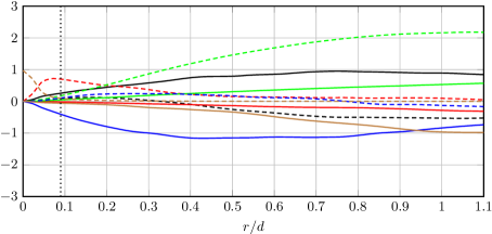
Note that the orientation-averaged non-linear inter-scale transfer rate, plotted with a minus sign as $-\Pi^{\prime a}$ ($\Pi^{\prime}\equiv\frac{\partial}{\partial r_{i}}\langle\delta u^{\prime}_{i}\delta{q^{\prime}}^{2}\rangle$), is not too significant in the range $0.4\leq r/d\leq 1.1$ at $(x_{1},x_{2})=(2d,0)$. However it is one of the four dominant terms in the range $\lambda/d\leq r/d\leq 0.4$ at this location. These four dominant terms are $-\mathcal{A}^{\prime a}$, $-\Pi^{\prime a}$, $\mathcal{P}_{\tilde{u}}^{\prime a}$ and $\mathcal{T}_{u^{\prime}}^{\prime a}$, and $\lambda$ is the Taylor microscale defined as $\lambda^{2}\equiv 2\langle u_{3}^{2}\rangle/\langle(\frac{\partial}{\partial x_{3}}u_{3})^{2}\rangle$. At $(x_{1},x_{2})=(2d,0)$ $\lambda$ is 0.09d and at $(x_{1},x_{2})=(8d,0)$ $\lambda$ is $0.15d$. The diffusion terms $\mathcal{D}_{x}^{\prime a}$ and $\mathcal{D}_{r}^{\prime a}$ effectively vanish at length-scales $r$ larger than $\lambda$, and they equal $\varepsilon^{\prime a}$ at $r=0$, as expected (see Valente & Vassilicos, 2015).

It is worth stressing that, at $(x_{1},x_{2})=(2d,0)$, the orientation-averaged non-linear inter-scale transfer rate $\Pi^{\prime a}$ is mainly balanced by the advection term $-\mathcal{A}^{\prime a}$ and coherent motion production and transport processes, i.e. $\mathcal{P}_{\tilde{u}}^{\prime a}$ and $\mathcal{T}_{\tilde{u}}^{\prime a}$, in the range $\lambda\leq r\leq 0.4d$. Even though energy spectra have well-defined power law ranges with exponents close to $-5/3$ at $(x_{1},x_{2})=(2d,0)$, $\Pi^{\prime a}$ is not constant with length-scale $r$.

Further downstream, at $(x_{1},x_{2})=(8d,0)$, the orientation-averaged non-linear inter-scale transfer rate $\Pi^{\prime a}$ is mainly balanced by the advection term $-\mathcal{A}^{\prime a}$ and coherent motion transport , i.e. $\mathcal{T}_{\tilde{u}}^{\prime a}$, in the range $\lambda\leq r\leq 0.3d$. All the other orientation-averaged terms in eq. 5 are less significant in this scale-range and at this position. The orientation-averaged impact of the coherent motions on the scale-by-scale budget eq. 5 gradually diminishes with increasing distance from the square prism. In the range $0.3d\leq r\leq 1.1d$ at $(x_{1},x_{2})=(8d,0)$, the dominant terms are now $-\mathcal{A}^{\prime a}$, $\mathcal{P}_{\tilde{u}}^{\prime a}$ and $-\Pi^{\prime a}$ which are all still positive, and $\mathcal{T}_{p^{\prime}}^{\prime a}$ which is still negative. The term $\mathcal{T}_{\tilde{u}}^{\prime a}$ has greatly reduced in relative importance from $(x_{1},x_{2})=(2d,0)$ to $(x_{1},x_{2})=(8d,0)$, but the presence of the pressure-velocity term $\mathcal{T}_{p^{\prime}}^{\prime a}$ has remained significant and about the same, if not even grown a little. Perhaps most striking of all is the fact that $-\Pi^{\prime a}$ has grown to become closer to an approximate constant fraction of $\varepsilon_{r}^{a}$ in the range $\lambda\leq r\leq 1.1d$ at $(x_{1},x_{2})=(8d,0)$ which is downstream of the point where the near $-5/3$ power law spectra appeared.

Figure 6: Orientation-averaged terms of eq. 6 (equivalently eq. 4) normalised by $\varepsilon_{r}^{a}$ at $x_{1}/d=2$ (top) and $x_{1}/d=8$ (bottom) on the geometric centreline. The vertical dotted line gives the position of $r=\lambda$.

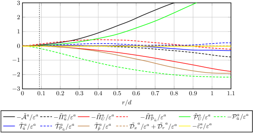
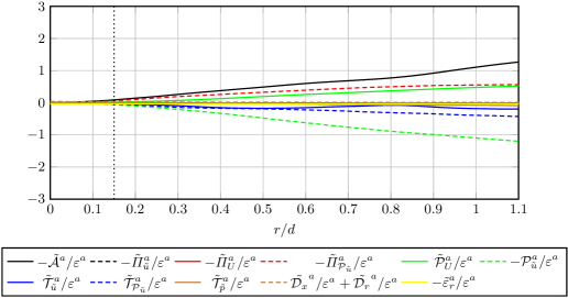
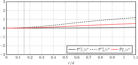
Production of stochastic fluctuation energy by mean flow gradients, namely $\mathcal{P}_{U}^{\prime a}$, is a minor contributor to the scale-by-scale stochastic fluctuation balance eq. 5 at $(x_{1},x_{2})=(2d,0)$ and effectively inexistent at $(x_{1},x_{2})=(8d,0)$ (see fig. 5). However, fig. 6 shows that production of coherent scale-by-scale energy by mean flow gradients, specifically $\mathcal{\tilde{P}}_{U}^{a}$ ($\mathcal{\tilde{P}}_{U}\equiv-\langle\delta\tilde{u}_{i}(\tilde{u}_{j}^{+}+\tilde{u}_{j}^{-})\rangle\frac{\partial\delta U_{i}}{\partial x_{j}}-2\langle\delta\tilde{u}_{i}\delta\tilde{u}_{j}\rangle\frac{\partial\delta U_{i}}{\partial r_{j}}$), is an important source of scale-by-scale energy in the coherent fluctuations balance eq. 6 at both positions $(x_{1},x_{2})=(2d,0)$ and $(8d,0)$. A clear picture emerges whereby, in an orientation-averaged sense, the mean flow gradients do not significantly feed the stochastic fluctuations directly but do feed the coherent motions which, in turn, feed the stochastic fluctuations via $\mathcal{P}_{\tilde{u}}^{\prime a}$. Indeed, the term $\mathcal{P}_{\tilde{u}}^{\prime a}$ appears as a dominant term in the orientation-averaged versions of both budgets eq. 5 and eq. 6 (see fig. 7, and also fig. 5 and fig. 6) but with opposite signs. This holds over a wide range of scales as small as $\lambda$ for the transfer of energy from the coherent to the stochastic fluctuations at $(x_{1},x_{2})=(2d,0)$ and as small as about $2\lambda$ or less for the production by mean flow gradients at $(x_{1},x_{2})=(2d,0)$ and for both $\mathcal{P}_{\tilde{u}}^{\prime a}$ and $\mathcal{\tilde{P}}_{U}^{a}$ at $(x_{1},x_{2})=(8d,0)$ (see figure fig. 7).

Figure 7: Orientation-averaged production terms normalised by $\varepsilon_{r}^{a}$ at $x_{1}/d=2$ (top) and $x_{1}/d=8$ (bottom) on the geometric centreline. The vertical dotted line gives the position of $r=\lambda$.

Figure 8: Orientation-averaged spatial transport terms normalised by $\varepsilon_{r}^{a}$ at $x_{1}/d=2$ (top) and $x_{1}/d=8$ (bottom) on the geometric centreline. The vertical dotted line gives the position of $r=\lambda$.

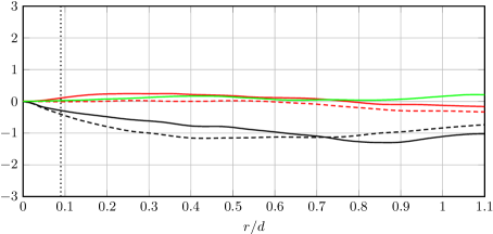
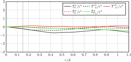
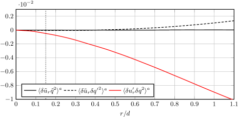
The terms in eq. 6 mostly decay with stream-wise distance from the prism along the centreline (see fig. 6), but they remain overall comparable to the terms in eq. 5 at the two positions $(x_{1},x_{2})$ examined here, particularly at length-scales $r\geq 0.2d$ or $0.3d$. Looking at eq. 8 and fig. 8 we can see that the orientation-averaged turbulent transport of $\delta q^{2}$ in physical space ($\mathcal{T}_{u}^{a}\equiv-{\frac{\partial\langle\frac{u_{i}^{+}+u_{i}^{-}}{2}\delta q^{2}\rangle}{\partial x_{i}}}$) is dominated by the orientation-averaged transport of stochastic fluctuations by coherent flow, i.e. $\mathcal{T}^{\prime a}_{\tilde{u}}$, at $(x_{1},x_{2})=(2d,0)$ over all plotted length-scales $r$ and at $(x_{1},x_{2})=(8d,0)$ up to $r/d\approx 0.5$. Indeed, the fluid between alternate coherent vortices (of opposite circulation) has large cross-stream velocities which dominate turbulent transport in space. $\mathcal{T}\textquoteright^{a}_{\tilde{u}}$ is negative because turbulent eddies smaller than the separation between these large-scale coherent vortices are transported away from the centreline. We expect this dominance of coherent flow transport to subside with downstream distance as the large coherent structures weaken.

((a))                                                                                                                     

((b))

Figure 9: Distribution of $\Pi^{\prime}$ and $\mathcal{T}_{p^{\prime}}^{\prime}$ normalised by $\varepsilon_{r}$ in scale space on the geometrical centreline at $x_{1}/d=8$ in (a) and (b), respectively.

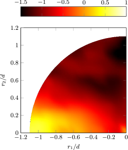
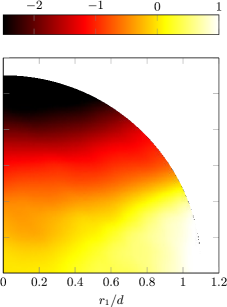
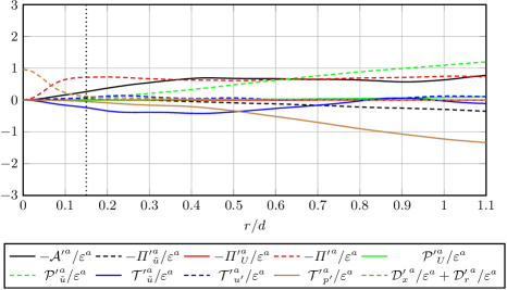
The results reported in this section concern orientation-averaged terms of equations (6) and (5). The picture is of course more complex if these orientation averages are lifted. For example, the orientation-averaged fully stochastic non-linear inter-scale transfer rate $\Pi^{\prime a}$ is negative at all length-scales $r$ sampled here, yet $\Pi^{\prime}$ can be either negative or positive in the $(r_{1},r_{2})$ plane, depending on orientation (see fig. 9). Similarly, the orientation-averaged fully stochastic pressure-velocity term $\mathcal{T}_{p^{\prime}}^{\prime a}$ is also negative at all the length-scales $r$ that we sampled, yet $\mathcal{T}_{p^{\prime}}^{\prime}$ can also be either negative or positive in the $(r_{1},r_{2})$ plane depending on orientation, as shown in fig. 9. The study of the distribution in the $(r_{1},r_{2})$ plane of the various terms in equations (6) and (5) is beyond this paper’s scope, but it is worth noting the correlation that seems to exist between $\Pi^{\prime}$ and $\mathcal{T}_{p^{\prime}}^{\prime}$: fig. 9 shows a significant tendency for these two terms to be positive or negative together. A correlation between fluctuations of the non-linear inter-scale transfer rate and the pressure-velocity term has also been observed in DNS of periodic turbulence by Yasuda & Vassilicos (2018) where it is discussed in more detail.

5 Effects of the Coherent motion and inhomogeneity on the Inter-scale Energy Transfer

Alves Portela et al. (2017) showed how the average non-linear inter-scale transfer rate of $\delta{q}^{2}$ is roughly constant when the orientations of $\mathbf{r}$ are averaged out in the $r_{3}=0$ plane, despite this transfer rate’s distribution being far from uniform in this plane. This was in fact observed in spite of the severe inhomogeneities and anisotropies evidenced in the previous section by the various non-zero terms in the KHMH equations (6) and (5), and even at $x_{1}/d=2$ (albeit for a small range of separations) where the coherent motions contribute a large portion of the total fluctuating kinetic energy (recall fig. 4). In this section we start by determining how this constancy of $\Pi^{a}$ observed in Alves Portela et al. (2017) and in Gomes-Fernandes et al. (2015) depends on contributions arising from the coherent and stochastic motions individually (§ 5.1), but also on statistical inhomogeneity (§ 5.2). We close the section by checking the signs of inter-scale fluxes in § 5.3.

5.1 Constant Non-linear Inter-scale Transfer as a Combined Effect

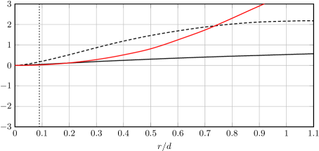
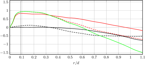
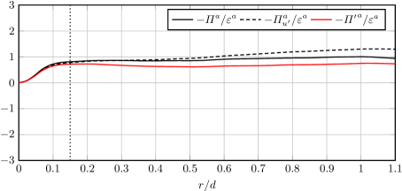
As mentioned in the previous section, the orientation-averaged inter-scale transfer rate of stochastic fluctuating energy by stochastic motions, $\Pi^{\prime a}$, is not independent of length-scale $r$ at $x_{1}/d=2$ on the centreline. However, fig. 10 shows that $\Pi_{u^{\prime}}^{a}$, the orientation-averaged inter-scale transfer rate of total fluctuating energy by the stochastic motions is close to being constant with $r$ in the range $\lambda<r<0.3d$ at this point ($x_{1}/d=2$, $x_{2}/d=0$). Furthermore, this approximate constant is closer to $-\varepsilon_{r}^{a}$ if $\Pi_{\tilde{u}}^{\prime a}$ is taken into account, i.e. at $(x_{1},x_{2})=(2d,0)$, $\Pi_{u^{\prime}}^{a}+\Pi_{\tilde{u}}^{\prime a}$ is also approximately constant in the range $\lambda<r<0.3d$ and closer to $-\varepsilon_{r}^{a}$ than $\Pi_{u^{\prime}}^{a}$. In fact, at this location, $\tilde{\Pi}_{\tilde{u}}^{a}\approx 0$ and eq. 9 reduces to

$$\Pi^{a}\approx\Pi_{u^{\prime}}^{a}+{\Pi_{\tilde{u}}^{\prime}}^{a}$$ (11)

in this range where $\Pi^{a}$ is approximately constant and close to $-\varepsilon_{r}^{a}$ (which is, in fact, very closely equal to $-\varepsilon$ in this range). This eq. 11 also holds further downstream on the centreline, but over a longer range of scales, e.g. $\lambda<r<d$ at $(x_{1},x_{2})=(8d,0)$ (see fig. 10).

The fact that a scale-range exists where $\Pi^{a}/\varepsilon^{a}_{r}$ is approximately constant and relatively close to $-1$ would not have been possible without the presence of coherent structures at $(x_{1},x_{2})=(2d,0)$. Whilst these coherent structures are non-dynamic in this scale-range, in the sense that $\tilde{\Pi}_{\tilde{u}}^{a}\approx 0$, they contribute to this clearly non-Kolmogorov yet Kolmogorov-sounding approximately constant value of $\Pi^{a}/\epsilon_{r}^{a}$ close to $-1$ in two ways: predominantly through $\Pi_{u^{\prime}}^{a}$ for the constancy of $\Pi^{a}/\varepsilon^{a}_{r}$, and through ${\Pi_{\tilde{u}}^{\prime}}^{a}$, the inter-scale transfer rate of stochastic energy by coherent fluctuations which improves the proximity of $\Pi^{a}/\varepsilon^{a}_{r}$ to $-1$.

Further downstream, at $(x_{1},x_{2})=(8d,0)$, $\Pi^{a}\approx\Pi_{u^{\prime}}^{a}$ in the range $\lambda<r<0.4d$. In this range and at this position, the orientation-averaged inter-scale transfer rate of stochastic energy by coherent fluctuations is zero, and the near-constancy with scale $r$ of $\Pi^{a}$ is in fact, to a significant extent, accountable to $\Pi^{\prime a}$, the orientation-averaged inter-scale transfer rate of stochastic energy by stochastic fluctuations (see fig. 5). But the coherent structures also contribute significantly because $\Pi^{a}$ is slightly but not insignificantly different from $\Pi^{\prime a}$, in such a way that $\Pi^{a}\approx\Pi_{u^{\prime}}^{a}$ is markedly closer to a constant than $\Pi^{\prime a}$ in this scale range; compare $\Pi^{\prime a}$ to $\Pi^{a}$ and $\Pi_{u^{\prime}}^{a}$ in fig. 11.

The orientation-averaged inter-scale transfer of total fluctuating energy by the stochastic fluctuations, $\Pi_{u^{\prime}}^{a}$, ceases to be constant at scales $r$ larger than $0.4d$: indeed, at this point $(x_{1},x_{2})=(8d,0)$, $-\Pi_{u^{\prime}}^{a}$ is an increasing positive function of $r$ in the range $0.4d<r<d$, mirroring the decrease of $-{\Pi_{\tilde{u}}^{\prime}}^{a}$ as a function of $r$ towards increasingly negative values (see fig. 10). These two contributions add up in eq. 11 to give a total inter-scale transfer rate $\Pi^{a}$ which is approximately constant over a range of scales extended well beyond $r=0.4d$, as evidenced in fig. 10. The correcting action of $-{\Pi^{\prime}_{\tilde{u}}}^{a}$ (orientation-averaged energy transfer rate of stochastic energy by coherent fluctuations), via its positive values at length-scales $r>0.4d$, is the essential ingredient for the extension of the near-constancy of $\Pi^{a}$ and its near-equality to $-\varepsilon$ over a range of scales which reaches as far out as $r=d$. Note that the fully stochastic inter-scale transfer rate $\Pi^{\prime a}$ also shows a tendency for being approximately constant over this range at $(x_{1},x_{2})=(8d,0)$ (see fig. 5) but its values are less close to $-\varepsilon$ and less constant than ${\Pi}^{a}_{u^{\prime}}+{\Pi^{\prime}_{\tilde{u}}}^{a}$. The coherent structures play a definite role in bringing $\Pi^{a}$ closer to a constant equal to $-\varepsilon$ at larger separations in this near-field flow.

In summary, at both locations $(x_{1},x_{2})=(2d,0)$ and $(8d,0)$, the reference equality

$$-{\Pi}^{a}_{u^{\prime}}-{\Pi^{\prime}_{\tilde{u}}}^{a}\approx\varepsilon^{a}_{r}$$ (12)

is not too far from our observations in the range where $\Pi^{a}\approx\mathrm{const}$. This equality re-writes $\Pi^{a}\approx\mathrm{const}$ with more information and this range increases as one moves downstream along the centreline reaching at least $\lambda<r<d$ at $(x_{1},x_{2})=(8d,0)$. We stress that eq. 12 is not exactly true. It might be more accurate to introduce a coefficient multiplying the right hand side $\varepsilon^{a}_{r}$ that is slightly smaller than 1 and not perfectly constant with $r$; but eq. 12 is an important reference formula for our discussion which is not concerned, at this stage, with exact details. The coherent structures play an important role in both terms of the left hand side of eq. 12 at both locations $(x_{1},x_{2})=(2d,0)$ and $(8d,0)$, but the stochastic fluctuations do too and more so at $(x_{1},x_{2})=(8d,0)$ than $(x_{1},x_{2})=(2d,0)$.

The approximate balance $\Pi^{a}\approx-\varepsilon$ may be reminiscent of a Kolmogorov equilibrium cascade but the Kolmogorov theory is applicable to statistically homogeneous equilibrium turbulence which is far from the kind of turbulence in the present near-field wake. This approximate balance follows here from the approximate balance eq. 12 and is partly supported by the effects of the coherent motions on the inter-scale turbulent energy transfers. The inter-scale transfer rate $\Pi^{a}$ must therefore depend on the inlet/boundary conditions because of the memory carried by the coherent motions, as it also of course depends on the kinetic energy and size of the local large scale turbulent eddies. It is therefore not possible to derive a scaling for $\Pi^{a}$ dimensionally, which means that it is not so easy to use the approximate balance $\Pi^{a}\approx-\varepsilon$ to derive a scaling for $\varepsilon$ either. One can derive a scaling for the turbulence dissipation rate in the context of Kolmogorov equilibrium turbulence precisely because the inter-scale transfer rate is taken to be independent of inlet/initial/boundary conditions in this context. Goto & Vassilicos (2016) have proposed a dissipation balance from which to derive turbulence dissipation scalings in non-stationary turbulence with a non-equilibrium cascade, and Alves Portela et al. (2018) have successfully adapted and applied this balance to the present near-field turbulent wake.

Figure 10: Orientation averaged non-linear inter-scale transfer terms from eqs. 4 and 3 normalised by $\varepsilon_{r}^{a}$ at $x_{1}/d=2$ (top) and $x_{1}/d=8$ (bottom). The vertical dotted line gives the position of $r=\lambda$.

Figure 11: Orientation-averaged inter-scale transfer terms normalised by $\varepsilon_{r}^{a}$ at $x_{1}/d=8$ on the geometric centreline. The vertical dotted line gives the position of $r=\lambda$.

5.2 Inhomogeneity Contributions to the Non-linear Inter-scale Energy Transfer

In interpreting our results, it is relevant to dissociate the potential contribution of inhomogeneity to the inter-scale transfer rates. Given that

$$\delta{\bf u}\delta q^{2}={\bf u}^{+}|{\bf u}^{+}|^{2}-{\bf u}^{-}|{\bf u}^{-}|^{2}+{\bf u}^{+}|{\bf u}^{-}|^{2}-{\bf u}^{-}|{\bf u}^{+}|^{2}-2\delta{\bf u}({\bf u}^{-}\cdot{\bf u}^{+})$$ (13)

one can see that statistical inhomogeneity can make a contribution to the average of $\delta{\bf u}\delta q^{2}$, at the very least from a non-zero average of ${\bf u}^{+}|{\bf u}^{+}|^{2}-{\bf u}^{-}|{\bf u}^{-}|^{2}$. However, we are mainly concerned with the non-linear inter-scale transfer rate ${\partial\over\partial r_{i}}(\delta u_{i}\delta q^{2})$ which has the property of being $0$ at ${\bf r}=0$ because it is equal to $\delta u_{i}{\partial\over\partial r_{i}}\delta q^{2}$ by incompressibility. We seek a decomposition of ${\partial\over\partial r_{i}}(\delta u_{i}\delta q^{2})$ into an inhomogeneity term and a term unaffected by inhomogeneity such that both vanish at ${\bf r}=0$. Given that ${\partial\over\partial r_{i}}(u^{+}_{i}|{\bf u}^{+}|^{2}-u^{-}_{i}|{\bf u}^{-}|^{2})={1\over 2}{\partial\over\partial\xi^{+}_{i}}(u^{+}_{i}|{\bf u}^{+}|^{2})+{1\over 2}{\partial\over\partial\xi^{-}_{i}}(u^{-}_{i}|{\bf u}^{-}|^{2})$ where $\xi^{+}_{i}=x_{i}+r_{i}/2$ and $\xi^{-}_{i}=x_{i}-r_{i}/2$, it is clear that ${\partial\over\partial r_{i}}(u^{+}_{i}|{\bf u}^{+}|^{2}-u^{-}_{i}|{\bf u}^{-}|^{2})$ is not $0$ at ${\bf r}=0$. We must therefore complement the inhomogeneity term ${\partial\over\partial r_{i}}(u^{+}_{i}|{\bf u}^{+}|^{2}-u^{-}_{i}|{\bf u}^{-}|)$ in such a way that the resulting inhomogeneity term cancels when ${\bf r}=0$. Starting from

$${\partial\over\partial r_{i}}(\delta u_{i}\delta q^{2})={\partial\over\partial r_{i}}[\delta u_{i}(|{\bf u}^{+}|^{2}+|{\bf u}^{-}|^{2})]-2{\partial\over\partial r_{i}}(\delta u_{i}{\bf u}^{-}\cdot{\bf u}^{+})$$ (14)

it rigorously follows that

$${\partial\over\partial r_{i}}(\delta u_{i}\delta q^{2})={1\over 2}{\partial\over\partial x_{i}}[u^{+}_{i}|{\bf u}^{+}|^{2}+u^{-}_{i}|{\bf u}^{-}|^{2}-u^{-}_{i}|{\bf u}^{+}|^{2}-u^{+}_{i}|{\bf u}^{-}|^{2}]-2{\partial\over\partial r_{i}}(\delta u_{i}{\bf u}^{-}\cdot{\bf u}^{+})$$ (15)

where both the inhomogeneity term ${1\over 2}{\partial\over\partial x_{i}}[u^{+}_{i}|{\bf u}^{+}|^{2}+u^{-}_{i}|{\bf u}^{-}|^{2}-u^{-}_{i}|{\bf u}^{+}|^{2}-u^{+}_{i}|{\bf u}^{-}|^{2}]$ and the inter-scale transfer term $-2{\partial\over\partial r_{i}}(\delta u_{i}{\bf u}^{-}\cdot{\bf u}^{+})$ vanish at ${\bf r}=0$ (by virtue of incompressibility in the case of the inter-scale transfer term). The average value of the inhomogeneity term, $4\Pi_{I}\equiv{1\over 2}{\partial\over\partial x_{i}}\langle u^{+}_{i}|{\bf u}^{+}|^{2}+u^{-}_{i}|{\bf u}^{-}|^{2}-u^{-}_{i}|{\bf u}^{+}|^{2}-u^{+}_{i}|{\bf u}^{-}|^{2}\rangle$ can be non-zero in inhomogeneous turbulence but equals zero in homogeneous turbulence. It is clear that $\Pi_{I}=0$ when the turbulence is statistically homogeneous. Unlike $\Pi_{I}$, the average value of the pure inter-scale term, $4\Pi_{H}\equiv-2{\partial\over\partial r_{i}}\langle\delta u_{i}{\bf u}^{-}\cdot{\bf u}^{+}\rangle$ can take non-zero values when the turbulence is statistically homogeneous.

We therefore have the decomposition

$$\Pi=\Pi_{I}+\Pi_{H}$$ (16)

where (i) all three terms ($\Pi$, $\Pi_{I}$ and $\Pi_{H}$) vanish at ${\bf r}=0$, (ii) $\Pi_{I}$ can only be non-zero in the presence of inhomogeneity and (iii) $\Pi_{H}$ has the exact same form as $\Pi$ in the case of homogeneous turbulence because $\frac{\partial\langle\delta u_{i}\delta q^{2}\rangle}{\partial r_{i}}=-2{\partial\over\partial r_{i}}\langle\delta u_{i}{\bf u}^{-}\cdot{\bf u}^{+}\rangle$ in such turbulence. This decomposition distinguishes between a term, $\Pi_{I}$, that is clearly directly accountable to spatial inhomogeneities, and an inter-scale transfer rate $\Pi_{H}$ which we may conjecture to be unaffected by spatial inhomogeneities. In relation to such a conjecture, we must ask whether our decomposition is unique.

Other such decompositions should take the form

$$\Pi=(\Pi_{I}+\Pi_{IH})+(\Pi_{H}-\Pi_{IH})$$ (17)

where $\Pi_{IH}$ must meet two conditions: (i) it must equal zero at ${\bf r}=0$ and (ii) it must vanish when the turbulence is statistically homogeneous. On account of this second condition, we write $\Pi_{IH}={\partial\over\partial x_{i}}\Phi^{x}_{i}$. Because we are dealing with third order statistics we assume that $\Phi^{x}_{i}$ can only be a sum of products of three velocity components and the most general way to write this is as follows:

$$\Phi^{x}_{i}=\alpha_{1}\langle u^{+}_{i}|{\bf u}^{+}|^{2}\rangle+\alpha_{2}\langle u^{+}_{i}{\bf u}^{-}\cdot{\bf u}^{+}\rangle+\alpha_{3}\langle u^{+}_{i}|{\bf u}^{-}|^{2}\rangle\\ +\beta_{1}\langle u^{-}_{i}|{\bf u}^{-}|^{2}\rangle+\beta_{2}\langle u^{-}_{i}{\bf u}^{-}\cdot{\bf u}^{+}\rangle+\beta_{3}\langle u^{-}_{i}|{\bf u}^{+}|^{2}\rangle$$ (18)

where $\alpha_{1}$, $\alpha_{2}$, $\alpha_{3}$, $\beta_{1}$, $\beta_{2}$, $\beta_{3}$ are dimensionless constants. With some care it easily follows that the condition $\Pi_{IH}=0$ for ${\bf r}=0$ implies

$$\alpha_{1}+\alpha_{2}+\alpha_{3}+\beta_{1}+\beta_{2}+\beta_{3}=0.$$ (19)

Given that $\Pi_{IH}$ contributes to the part $(\Pi_{H}-\Pi_{IH})$ of the decomposition, it must be possible to express it in the form $\Pi_{IH}={\partial\over\partial r_{i}}\Phi^{r}_{i}$. To find the conditions for this to be possible, we use ${\partial\over\partial x_{i}}={\partial\over\partial\xi^{+}_{i}}+{\partial\over\partial\xi^{-}_{i}}$ and use $\Pi_{IH}={\partial\over\partial x_{i}}\Phi^{x}_{i}$ to write

$$\Pi_{IH}=\alpha_{1}{\partial\over\partial\xi^{+}_{i}}\langle u^{+}_{i}|{\bf u}^{+}|^{2}\rangle+\alpha_{2}{\partial\over\partial\xi^{+}_{i}}\langle u^{+}_{i}{\bf u}^{-}\cdot{\bf u}^{+}\rangle+\beta_{2}{\partial\over\partial\xi^{+}_{i}}\langle u^{-}_{i}{\bf u}^{-}\cdot{\bf u}^{+}\rangle+\beta_{3}{\partial\over\partial\xi^{+}_{i}}\langle u^{-}_{i}|{\bf u}^{+}|^{2}\rangle\\ +\alpha_{2}{\partial\over\partial\xi^{-}_{i}}\langle u^{+}_{i}{\bf u}^{-}\cdot{\bf u}^{+}\rangle+\alpha_{3}{\partial\over\partial\xi^{-}_{i}}\langle u^{+}_{i}|{\bf u}^{-}|^{2}\rangle+\beta_{1}{\partial\over\partial\xi^{-}_{i}}\langle u^{-}_{i}|{\bf u}^{-}|^{2}\rangle+\beta_{2}{\partial\over\partial\xi^{-}_{i}}\langle u^{-}_{i}{\bf u}^{-}\cdot{\bf u}^{+}\rangle.$$ (20)

Note that $\alpha_{1}{\partial\over\partial\xi^{+}_{i}}\langle u^{+}_{i}|{\bf u}^{+}|^{2}\rangle=2\alpha_{1}{\partial\over\partial r_{i}}\langle u^{+}_{i}|{\bf u}^{+}|^{2}\rangle$ because ${\partial\over\partial\xi^{-}_{i}}\langle u^{+}_{i}|{\bf u}^{+}|^{2}\rangle=0$ and ${\partial\over\partial r_{i}}={1\over 2}({\partial\over\partial\xi^{+}_{i}}-{\partial\over\partial\xi^{-}_{i}})$. For the same reason, $\beta_{1}{\partial\over\partial\xi^{-}_{i}}\langle u^{-}_{i}|{\bf u}^{-}|^{2}\rangle=-2\beta_{1}{\partial\over\partial r_{i}}\langle u^{-}_{i}|{\bf u}^{-}|^{2}\rangle$. All the other terms and combinations of other terms cannot be rephrased in ${\partial\over\partial r_{i}}$ form. The necessary form $\Pi_{IH}={\partial\over\partial r_{i}}\Phi^{r}_{i}$ then implies $\alpha_{2}=\alpha_{3}=\beta_{2}=\beta_{3}=0$. From eq. 19 follows $\alpha_{1}=-\beta_{1}$ and therefore

$$\Pi_{IH}=\alpha{\partial\over\partial r_{i}}(\langle u^{+}_{i}|{\bf u}^{+}|^{2}\rangle+\langle u^{-}_{i}|{\bf u}^{-}|^{2}\rangle)=\alpha{\partial\over\partial x_{i}}(\langle u^{+}_{i}|{\bf u}^{+}|^{2}\rangle-\langle u^{-}_{i}|{\bf u}^{-}|^{2}\rangle).$$ (21)

where we also made use of $\Pi_{IH}={\partial\over\partial x_{i}}\Phi^{x}_{i}$ with eq. 18 and eq. 19, and where we set $\alpha\equiv 2\alpha_{1}$.

In conclusion, the decomposition eq. 16 is not unique as one can always use $\Pi_{IH}$ given by eq. 21 to obtain another equally valid decomposition eq. 17. However, if one averages over scale-space orientations, the decomposition

$$\Pi^{a}=\Pi_{I}^{a}+\Pi_{H}^{a}$$ (22)

is unique because $\Pi_{IH}^{a}=0$ given that $\Pi_{IH}$ in eq. 21 is such that $\Pi_{IH}({\bf r})=-\Pi_{IH}(-{\bf r})$. The conjecture that the orientation-averaged inter-scale transfer rate $\Pi_{H}^{a}$ may be unaffected by spatial inhomogeneities is more likely to hold than the conjecture that $\Pi_{H}$ is unaffected by spatial inhomogeneities. This conjecture and the decomposition introduced in this subsection are an attempt at introducing a tool which can help make some analytic sense of the concept of an inhomogeneous turbulence cascade.

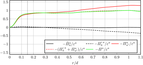
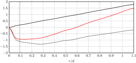
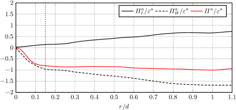
In fig. 12 we plot the orientation averaged inter-scale transfer rates $\Pi^{a}$, $\Pi_{I}^{a}$ and $\Pi_{H}^{a}$ at the two centreline positions $(x_{1},x_{2})=(2d,0)$ and $(8d,0)$. Inhomogeneity inter-scale transfer is present and positive at all scales, but may be considered negligible at dissipative scales $r$ smaller than $0.1d$, i.e. smaller than the Taylor microscale $\lambda$. However, it does make a significant contribution to the total inter-scale energy transfer rate $\Pi^{a}$ at scales $r$ larger than $\lambda$, particularly at $(x_{1},x_{2})=(2d,0)$ where $\Pi_{I}^{a}$ is commensurate throughout these scales with the negative inter-scale transfer $\Pi_{H}^{a}$. In fact $\Pi^{a}$ changes sign from negative to positive as $r$ increases beyond $r\approx 0.6d$ because of the influence of the positive inhomogeneity inter-scale energy transfer rate.

In fig. 12 one can also see that the contribution of the inhomogeneity part of the inter-scale energy transfer weakens with downstream distance, while remaining positive throughout the scales. $\Pi^{a}$ and $\Pi_{H}^{a}$ are both negative throughout the scales and significantly closer to each other than to $\Pi_{I}^{a}$ at $(x_{1},x_{2})=(8d,0)$, which is not the case at $(x_{1},x_{2})=(2d,0)$.

It is particularly intriguing that $\Pi^{a}$ would not have been approximately constant across the scales, from about $\lambda$ to about $0.3d$ at $(x_{1},x_{2})=(2d,0)$ and from about $\lambda$ to about $d$ at $(x_{1},x_{2})=(8d,0)$, without the inhomogeneity contribution coming from $\Pi_{I}^{a}$. It is in fact this inhomogeneity contribution which returns a near-constancy of $\Pi^{a}$ all the way up to scales $r$ equal to $d$ at $(x_{1},x_{2})=(8d,0)$ and imparts on the orientation-averaged inter-scale energy transfer $\Pi^{a}$ a Kolmogorov-seeming behaviour over a decade of scales $r$.

The results of these two subsections suggest that the approximate balance $\Pi^{a}\approx-\varepsilon$ observed in our turbulent wake’s very near field, even if reminiscent of a Kolmogorov equilibrium for homogeneous turbulence, is in fact possible in this near-field turbulence because of the presence of spatial inhomogeneity and coherent structures.

Figure 12: Orientation averaged inter-scale energy transfer terms $\Pi_{I}^{a}$, $\Pi_{H}^{a}$ and $\Pi^{a}$ (see equations 15 and 16) at $x_{1}/d=2$ (top) and $x_{1}/d=8$ (bottom). The vertical dotted line gives the position of $r=\lambda$.

5.3 Inter-scale fluxes

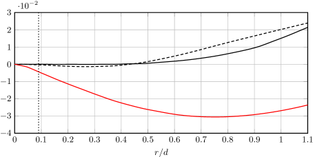
In order to interpret the inter-scale physics behind the negative sign of $\Pi^{a}$ it is necessary to also consider the inter-scale flux $\langle\delta{\bf u}\delta q^{2}\rangle$ given that $\Pi$ is the divergence of this flux in scale space ${\bf r}$. In particular, it is necessary to consider the sign of the radial component of the orientation-averaged inter-scale flux. One cannot claim that the inter-scale energy transfer proceeds from large to small scales on average if this sign is not negative too.

The inter-scale flux vectors which correspond to each term in eq. 7 are related by

$$\langle\delta{\bf u}\delta q^{2}\rangle=\langle\delta{\bf u}^{\prime}\delta q^{\prime 2}\rangle+\langle\delta{\bf\tilde{u}}\delta q^{\prime 2}\rangle+\langle\delta{\bf\tilde{u}}\delta\tilde{q}^{2}\rangle+2\langle\delta{\bf u}^{\prime}(\delta{\bf u}^{\prime}\cdot\delta{\bf\tilde{u}})\rangle.$$ (23)

The flux vectors are placed in this equation in exactly the same way as their corresponding inter-scale transfer rates are placed in eq. 7. The inter-scale flux identity which reflects $\tilde{\Pi}_{\mathcal{P}_{\tilde{u}}}=\Pi_{u^{\prime}}-\Pi^{\prime}$ is $2\langle\delta{\bf u}^{\prime}(\delta{\bf u}^{\prime}\cdot\delta{\bf\tilde{u}})\rangle=\langle\delta{\bf u}^{\prime}\delta q^{2}\rangle-\langle\delta{\bf u}^{\prime}\delta q^{\prime 2}\rangle$. Combined with eq. 23 it yields

$$\langle\delta{\bf u}\delta q^{2}\rangle=\langle\delta{\bf u}^{\prime}\delta q^{2}\rangle+\langle\delta{\bf\tilde{u}}\delta q^{\prime 2}\rangle+\langle\delta{\bf\tilde{u}}\delta\tilde{q}^{2}\rangle$$ (24)

which corresponds to eq. 9.

We are interested in the orientation-averaged radial components of these fluxes in the $r_{3}=0$ plane. In fig. 13 we plot, as functions of $r$, the orientation-averaged radial components (in the $r_{3}=0$ plane) $\langle\delta{u^{\prime}}_{r}\delta{q}^{2}\rangle^{a}$, $\langle\delta\tilde{u}_{r}\delta{q^{\prime}}^{2}\rangle^{a}$ and $\langle\delta\tilde{u}_{r}\delta\tilde{q}^{2}\rangle^{a}$. The latter is zero where eq. 12 is relevant. Concentrating our attention on the scale range where eq. 12 is relevant, the signs of these orientation-averaged radial fluxes and of the corresponding orientation-averaged inter-scale transfer rates therefore suggest the following: (i) concerning $\Pi_{u^{\prime}}^{a}$, the stochastic fluctuations transfer, on average, total (stochastic and coherent) fluctuating energy from large to small scales in the range $r<0.3d$ at $(x_{1},x_{2})=(2d,0)$ and $r<d$ at $(x_{1},x_{2})=(8d,0)$; (ii) concerning ${\Pi^{\prime}_{\tilde{u}}}^{a}$, the coherent fluctuations transfer, on average, stochastic energy from large to small scales at length-scales $r<0.3d$ at both spatial locations, but from small to large scales at $(x_{1},x_{2})=(8d,0)$ in the range $0.4d<r<d$. The contribution of ${\Pi^{\prime}_{\tilde{u}}}^{a}$ is the smallest of the two inter-scale transfer rate terms, $\Pi_{u^{\prime}}^{a}$ and ${\Pi^{\prime}_{\tilde{u}}}^{a}$, in eq. 11 and eq. 12. The inter-scale fluctuating energy transfer proceeds, therefore, from large to small scales on average, mostly because of the large to small scale transfer of total fluctuating energy by stochastic fluctuations.

Figure 13: Orientation averaged non-linear inter-scale radial fluxes terms at $x_{1}/d=2$ (top) and $x_{1}/d=8$ (bottom). The vertical dotted line gives the position of $r=\lambda$.

6 Conclusions

By conditionally sampling the fluctuating velocity and pressure fields in the wake generated by a square prism (as introduced in the classical work of Hussain & Reynolds (1970)), those fluctuating fields were decomposed into two components: a phase averaged component whose time signature follows the vortex shedding and a stochastic component which can be interpreted as the turbulent fluctuations which are superimposed onto the organised motion associated with the vortex shedding. Taking also into account the corresponding mean fields, we used the inter-scale and inter-space energy balance, the KHMH equation, written for a triple decomposition and we analysed DNS data of a near-field turbulent wake. Our study has been limited to the geometric centreline and the plane of the mean flow. The turbulence in this near wake, at a distance between $2d$ and $8d$ of the square prism, is very inhomogeneous and very unsteady. Unsurprisingly, the non-stationarity and inhomogeneity contributions to the KHMH balance dominate. The pressure-velocity term is sizeable too, particularly at scales $r$ larger than about $0.4d$, and has an orientation signature which appears similar to that of the purely stochastic non-linear inter-scale transfer rate.

We reduced the amount of information by taking orientation averages of every term in the KHMH equation. In an orientation-averaged sense, the production of kinetic energy by the mean flow does not feed the stochastic turbulent fluctuations directly. Instead, energy is transferred from the mean flow to the coherent fluctuations which in turn transfer energy to the stochastic fluctuations. The coherent structures also dominate spatial turbulent transport of small-scale two-point stochastic turbulent fluctuations.

Alves Portela et al. (2017) found that the orientation-averaged non-linear inter-scale transfer rate $\Pi^{a}$ is approximately independent of $r$ in the scale-ranges $\lambda\leq r\leq 0.3d$ and $\lambda\leq r\leq d$, respectively, at stream-wise distances $x_{1}=2d$ and $x_{1}=8d$ from the square prism. We have shown here that this requires a definite inter-scale transfer contribution by the coherent structures at $x_{1}=2d$ but not at $x_{1}=8d$ where it is mostly attributable to stochastic fluctuations. However, at $x_{1}=8d$, $-\Pi^{a}$ is also very close to $\varepsilon$ in the range $\lambda\leq r\leq d$ and the contribution of the coherent structure’s inter-scale energy transfer is a significant factor in achieving this approximate equality. The later contribution, albeit relatively small, appears to resist the energy transfer in the direct sense since ${\Pi^{\prime}_{\tilde{u}}}^{a}>0$ at large enough scales. The self-interaction of the coherent motions plays a negligible role in the inter-scale energy transfer.

The inter-scale energy transfer rate can be decomposed in two terms, one which is absent in homogeneous turbulence and therefore relates directly to spatial inhomogeneity, and another which remains present in homogeneous turbulence. One might be able to consider the concept of inhomogeneity-induced inter-scale energy transfers alongside the usual homogeneous inter-scale energy transfers. Perhaps most surprisingly and most importantly, a very significant direct contribution to the inter-scale energy transfer rate turns out to come from spatial inhomogeneity without which the approximate equality $-\Pi^{a}\approx\varepsilon$ would not have been possible in this very near field..

References

- Alves Portela et al. (2017) Alves Portela, F., Papadakis, G. & Vassilicos, J. C. 2017 The turbulence cascade in the near wake of a square prism. Journal of Fluid Mechanics 825, 315–352.
- Alves Portela et al. (2018) Alves Portela, F., Papadakis, G. & Vassilicos, J. C. 2018 Turbulence dissipation and the role of coherent structures in the near wake of a square prism. Phys. Rev. Fluids 3, 124609.
- Braza et al. (2006) Braza, M., Perrin, R. & Hoarau, Y. 2006 Turbulence properties in the cylinder wake at high Reynolds numbers. Journal of Fluids and Structures 22 (6-7), 757–771.
- Davies (1976) Davies, M. E. 1976 A comparison of the wake structure of a stationary and oscillating bluff body, using a conditional averaging technique. Journal of Fluid Mechanics 75 (02), 209.
- Duchon & Robert (2000) Duchon, J. & Robert, R. 2000 Inertial energy dissipation for weak solutions of incompressible Euler and Navier-Stokes equations. Nonlinearity 13 (1), 249–255.
- Feldman (2011) Feldman, M. 2011 Hilbert Transform Applications in Mechanical Vibration. John Wiley & Sons.
- Frisch (1995) Frisch, U. 1995 Turbulence: The Legacy of A. N. Kolmogorov. Cambridge University Press.
- Gomes-Fernandes et al. (2015) Gomes-Fernandes, R., Ganapathisubramani, B. & Vassilicos, J. C. 2015 The energy cascade in near-field non-homogeneous non-isotropic turbulence. Journal of Fluid Mechanics 771, 676–705.
- Goto & Vassilicos (2016) Goto, S. & Vassilicos, J. C. 2016 Unsteady turbulence cascades. Physical Review E - Statistical, Nonlinear, and Soft Matter Physics 94 (5), 1–3.
- Hill (1997) Hill, R. J. 1997 Applicability of Kolmogorov’s and Monin’s equations of turbulence. Journal of Fluid Mechanics 353, 67–81.
- Hill (2001) Hill, R. J. 2001 Equations relating structure functions of all orders. Journal of Fluid Mechanics 434, 379–388.
- Hill (2002a) Hill, R. J. 2002a Exact second-order structure-function relationships. Journal of Fluid Mechanics 468, 317–326.
- Hill (2002b) Hill, R. J. 2002b The Approach of Turbulence to the Locally Homogeneous Asymptote as Studied using Exact Structure-Function Equations. Arxiv pp. 1–24, arXiv: 0206034.
- Hussain (1983) Hussain, A. K. M. F. 1983 Coherent structures—reality and myth. Physics of Fluids 26 (10), 2816.
- Hussain et al. (1987) Hussain, A. K. M. F., Jeong, J. & Kim, J. 1987 Structure of turbulent shear flows. In Center for Turbulent Research. Proceedings of the summer program 1987.
- Hussain & Reynolds (1970) Hussain, A. K. M. F. & Reynolds, W. C. 1970 The mechanics of an organized wave in turbulent shear flow. Journal of Fluid Mechanics 41 (02), 241–258.
- Lyn et al. (1995) Lyn, D. A., Einav, S., Rodi, W. & Park, J. H. 1995 A laser-Doppler velocimetry study of ensemble-averaged characteristics of the turbulent near wake of a square cylinder. Journal of Fluid Mechanics 304, 285.
- Marati et al. (2004) Marati, N., Casciola, C. M. & Piva, R. 2004 Energy cascade and spatial fluxes in wall turbulence. Journal of Fluid Mechanics 521, 191–215.
- Reynolds & Hussain (1972) Reynolds, W. C. & Hussain, A. K. M. F. 1972 The mechanics of an organized wave in turbulent shear flow. Part 3. Theoretical models and comparisons with experiments. Journal of Fluid Mechanics 54 (02), 263.
- Thiesset et al. (2014) Thiesset, F., Danaila, L. & Antonia, R. A. 2014 Dynamical interactions between the coherent motion and small scales in a cylinder wake. Journal of Fluid Mechanics 749 (April 2016), 201–226.
- Valente & Vassilicos (2015) Valente, P. C. & Vassilicos, J. C. 2015 The energy cascade in grid-generated non-equilibrium decaying turbulence. Physics of Fluids 27 (4), 045103.
- Wlezien & Way (1979) Wlezien, R. W. & Way, J. L. 1979 Techniques for the experimental investigation of the near wake of a circular cylinder. AIAA Journal 17 (6), 563–570.
- Yasuda & Vassilicos (2018) Yasuda, T. & Vassilicos, J. C. 2018 Spatio-temporal intermittency of the turbulent energy cascade. Journal of Fluid Mechanics 853, 235–252.