Broadband Synchronization and Compressive Channel Estimation for Hybrid mmWave MIMO Systems

Abstract

Synchronization is a fundamental procedure in cellular systems whereby an user equipment (UE) acquires the time and frequency information required to decode the data transmitted by a base station (BS). Due to the necessity of using large antenna arrays to obtain the beamforming gain required to compensate for small antenna aperture, synchronization must be performed either jointly with beam training as in 5G New Radio (NR), or at the low signal-to-noise ratio (SNR) regime if the high-dimensional millimeter wave (mmWave) multiple-input multiple-output (MIMO) channel is to be estimated. To circumvent this problem, this work proposes the first synchronization framework for mmWave MIMO that is robust to both timing offset (TO), carrier frequency offset (CFO), and phase noise (PN) synchronization errors and, unlike prior work, implicitly considers the use of multiple RF chains at both transmitter and receiver. I provide a theoretical analysis of the estimation problem and derive the hybrid Cramér-Rao lower bound (HCRLB) for the estimation of both the CFO, PN, and equivalent beamformed channels seen by the different receive RF chains. I also propose two novel algorithms to estimate the different unknown parameters, which rely on approximating the minimum mean square error (MMSE) estimator for the PN and the maximum likelihood (ML) estimators for both the CFO and the equivalent beamformed channels. Thereafter, I propose to use the estimates for the equivalent beamformed channels to perform compressive estimation of the high-dimensional frequency-selective mmWave MIMO channel and thus undergo data transmission. For performance evaluation, I consider the QuaDRiGa channel simulator, which implements the 5G NR channel model, and show that both compressive channel estimation without prior synchronization is possible, and the proposed approaches outperform current solutions for joint beam training and synchronization currently considered in 5G NR.

I Introduction

Time-frequency synchronization is one of the most important design aspects in cellular systems. In mmWave systems, however, acquiring synchronization information is significantly more challenging than for traditional sub-$6$ GHz MIMO systems. Due to the necessity of using large antenna arrays to obtain the beamforming gain required to compensate for small antenna aperture, time and frequency synchronization must be performed either jointly with beam training as in 5G NR, or at the low SNR regime if the high-dimensional mmWave MIMO channel is to be estimated. Unfortunately, at such high operating frequency bands, synchronization, channel estimation, and data transmission are impacted by PN impairments, which consist of random fluctuations in the phase of the carrier generated by local oscillators.

I-A Prior work and Motivation

In the context of mmWave MIMO systems, synchronization parameters need to be properly estimated and compensated for before channel state information (CSI) can be acquired. This sets new challenges as synchronization acquisition must be performed at the low SNR regime, before transmit and receive communication beams can be aligned for data transmission.

The problem of compressed sensing (CS)-based joint beam training and synchronization is studied in [1, 2]. In [1], the problem of beam training under PN errors and unknown CFO was studied for narrowband mmWave MIMO systems using analog architectures. Therein, an extended Kalman filter (EKF)-based solution is proposed to track the joint phase of the unknown PN and beamformed narrowband channel, the phase of the received signal is compensated, and then matching pursuit (MP) is used to estimate the dominant angle-of-departure (AoD) and angle-of-arrival (AoA), thereby discovering a single communication path. In [2], a compressive initial access approach based on omnidirectional pseudorandom analog beamforming is proposed as an alternative to the directional initial access procedure used during beam management in 5G NR, and the effects of imperfect TO and CFO are studied therein. The main limitations of the algorithm proposed in [2] are: i) the algorithm is tailored to line-of-sight (LOS) channel models, thereby implicitly ignoring the presence of spatio-temporal clusters in the propagation environment; ii) the proposed signal model assumes the presence of phase measurement errors only due to CFO, thereby ignoring the PN impairment. Prior work on joint broadband channel estimation and synchronization for mmWave MIMO is limited, since much (if not most) of the prior work on channel estimation assumes perfect synchronization at the receiver side [3], [4], [5], [6], [7].

In the context of broadband channel models, prior work is limited to [8, 9, 10, 11]. In [8], the problem of joint channel and PN estimation for a single-input single-output (SISO) system is considered, which is unrealistic at mmWave, and the proposed algorithms are only evaluated in very high SNR regime. In [9], analog-only architectures with a single RF chain are assumed, and an autocorrelation-based iterative algorithm is proposed to jointly estimate the CFO and the mmWave channel. Prior work in [9] assumes that analog beamformers and combiners can be instantaneously reconfigured for two consecutive transmitted time-domain samples, which is unrealistic since phase-shifters need an adjustment time for phase reconfiguration [12]. Further, the algorithm proposed in [9] has only been evaluated for mmWave channels having a very small number of non-clustered multipath components, which is not realistic at mmWave [13]. In addition, owing to the nature of the autocorrelation function, the proposed algorithm does not perform both well when the CFO is considerably large and the SNR is low. In [10], a CFO-robust beam alignment technique is developed to find the beam pairs maximizing the received SNR. The main limitation of [10] is that the algorithm proposed therein can only be applied to analog MIMO architectures, and its CFO correction capability is limited by both the number of delay taps in the mmWave MIMO channel, as well as the length of the training sequence, thereby making the algorithm impractical for practical mmWave deployments with more significant CFO. In [11], the joint CFO and broadband channel estimation problem is formulated as a sparse bilinear optimization problem, which is solved using the parametric bilinear generalized approximate message passing (PBiGAMP) algorithm in [14]. The main limitation of [11] is that the proposed estimation strategy is tailored to all-digital MIMO architectures with low-resolution analog-to-digital converter (ADC) converters, thereby not being directly applicable to hybrid MIMO architectures. In [15], a similar strategy to the one in [11] is followed, in which the joint CFO and channel estimation problem is studied for all-digital MIMO architectures. The problem is formulated as a quantized sparse bilinear optimization problem, which is solved using sparse lifting to increase the dimension of the CFO and channel estimation problem [16], and then applying the generalized approximate message passing (GAMP) algorithm in [17] to solve the lifted problem.

II Contributions

In this paper, I develop efficient and robust solutions to the problem of estimating the TO, CFO, PN, and frequency-selective channel for hybrid mmWave MIMO systems. The proposed solutions can leverage the spatial design degrees of freedom brought by having several RF chains at both the transmitter and receiver to perform synchronization and compressive channel estimation, without relying on any prior channel knowledge. The contributions of this paper are summarized hereinafter:

• Based on a protocol of forwarding several training frames from the transmitter to the receiver [18], [2], [3], [19], I formulate and find a solution to the problem of TO, CFO, PN and frequency-selective mmWave MIMO channel estimation for systems employing hybrid architectures. Further, the focus is on analyzing the synchronization problem at the low SNR regime.

• I propose to forward several training frames using Zadoff-Chu (ZC)-based beamforming in combination with random subarray switching and antenna selection in order to both acquire synchronization and enable compressive channel estimation at the low SNR regime.

• For every training frame, which comprises several orthogonal frequency division multiplexing (OFDM) symbols, as in the 5G NR wireless standard [20], I theoretically analyze the hybrid Cramér-Rao lower bound (CRLB) for the problem of estimating the CFO, PN, and equivalent frequency-selective beamformed channel collecting the joint effect of the transmit hybrid precoders, frequency-selective mmWave MIMO channel, receive hybrid combiners, and equivalent transmit-receive pulse-shaping that bandlimits the complex baseband equivalent channel.

• I propose two novel iterative algorithms based on the expectation-maximization (EM) method, which aim at finding the ML estimates for the CFO and beamformed equivalent channels, as well as the linear minimum mean square error (LMMSE) estimates for the PN samples that impair the receive signals. The first proposed algorithm exhibits very good performance, yet it exhibits high computational complexity. The second proposed algorithm, conversely, offers a trade-off between estimation performance and computational complexity, and exhibits a very small performance gap with respect to the first algorithm.

• Using estimates of the unknown parameters for every training frame, I formulate the problem of estimating the high-dimensional frequency-selective mmWave MIMO channel, and find a solution to this problem using a variation of the simultaneous weighted - orthogonal matching pursuit (SW-OMP) algorithm in [21].

I evaluate the performance of the proposed algorithms in terms of normalized mean square error (NMSE) and spectral efficiency. I use all-digital precoders and combiners to show the effectiveness of the proposed algorithms. Simulation results obtained from the estimated channel show that both the TO, CFO, and equivalent channels can be accurately estimated even in the presence of strong PN, and when the MIMO channel has several clusters with non-negligible angular spread (AS). Furthermore, I show that near-optimum spectral efficiency can be attained, without incurring in significant overhead and/or computational complexity. To the best of my knowledge, this is the first work that theoretically analyzes and provides solutions to the problem of joint synchronization and compressive channel estimation at mmWave considering hybrid MIMO architectures, and that is robust to both CFO, PN, and low SNR regime.

III System model with synchronization impairments

I consider a single-user mmWave MIMO-OFDM communications link in which a transmitter equipped with $N_{\mathrm{t}}$ antennas sends $N_{\mathrm{s}}$ data streams to a receiver having $N_{\mathrm{r}}$ antennas. Both transmitter and receiver are assumed to use partially-connected hybrid MIMO architectures [22], as shown in Fig. 1, with $L_{\mathrm{t}}$ and $L_{\mathrm{r}}$ RF chains. A frequency-selective hybrid precoder is used at the transmitter, with $\bm{\mathsf{F}}[k]=\bm{\mathsf{F}}_{\text{RF}}\bm{\mathsf{F}}_{\text{BB}}[k]\in{\mathbb{C}}^{N_{\mathrm{t}}\times N_{\mathrm{s}}}$, where $\bm{\mathsf{F}}_{\text{RF}}\in\mathbb{C}^{N_{\mathrm{t}}\times L_{\mathrm{t}}}$ is the analog precoder and $\bm{\mathsf{F}}_{\text{BB}}[k]\in\mathbb{C}^{L_{\mathrm{t}}\times N_{\mathrm{s}}}$ is the digital one at subcarrier $k$, $0\leq k\leq K-1$. The Radio-Frequency (RF) precoder and combiner are implemented using a partially-connected network of phase-shifters and switches, as described in [22]. Likewise, the receiver applies a hybrid linear combiner $\bm{\mathsf{W}}[k]=\bm{\mathsf{W}}_{\text{RF}}\bm{\mathsf{W}}_{\text{BB}}[k]\in{\mathbb{C}}^{N_{\mathrm{r}}\times L_{\mathrm{r}}}$, where $\bm{\mathsf{W}}_{\text{RF}}\in\mathbb{C}^{N_{\mathrm{r}}\times L_{\mathrm{r}}}$ is the analog combiner, and $\bm{\mathsf{W}}_{\text{BB}}[k]\in\mathbb{C}^{L_{\mathrm{r}}\times N_{\mathrm{s}}}$ is the baseband combiner at the $k$-th subcarrier.

Without loss of generality, I assume that the transmitted signal comprises $N_{\mathrm{tr}}$ OFDM symbols with a cyclic prefix (CP) of length $L_{\mathrm{c}}$, similarly to the 5G NR wireless standard [20]. Let us define the rectangular pulse-shape $w_{N}[n]=1$ for $n\in[0,N-1]$, and $w_{N}[n]=0$ otherwise. Then, the hybrid-precoded transmitted signal can be expressed as

$$\begin{split}{\mathbf{x}}[n]&=\frac{1}{K}\bm{\mathsf{F}}_{\text{RF}}\sum_{k=0}^{K-1}\sum_{t=0}^{N_{\mathrm{tr}}-1}\bm{\mathsf{F}}_{\text{BB}}[k]{\bm{\mathsf{s}}}_{t}[k]e^{{\mathsf{j}}\frac{2\pi k(n-L_{\mathrm{c}}-t(K+L_{\mathrm{c}}))}{K}}w_{K+L_{\mathrm{c}}}[n-t(K+L_{\mathrm{c}})],\\ &\quad n=0,\ldots,(N_{\mathrm{tr}}-1)(K+L_{\mathrm{c}})-1,\end{split}$$ (1)

Then, let $n_{0}\in\mathbb{K}_{+}$, $\Delta f\in\mathbb{R}$, $\theta[n]\in\mathbb{R}$ denote the unknown TO, CFO normalized to the sampling rate $f_{\text{s}}=1/T_{\mathrm{s}}$, and $n$-th receive PN sample. Also, let $\{{\mathbf{W}}[\ell]\}_{\ell=0}^{K-1}$ denote the time-domain hybrid combiner, given by the IFFT of the frequency-selective hybrid combiner $\{\bm{\mathsf{W}}[k\}_{k=0}^{K-1}$. Then, the received signal at discrete time instant $n$ can be written as

$${\mathbf{y}}[n]=\left\{{\mathbf{W}}^{*}[\ell]\right\}_{\ell=0}^{K-1}*\left(\sum_{d=0}^{D-1}{\mathbf{H}}[d]{\mathbf{x}}[n-d-n_{0}]e^{{\mathsf{j}}(2\pi\Delta fn+\theta[n])}\right)+{\mathbf{v}}[n],$$ (2)

for $n=0,\ldots,N+D+n_{0}-1$, with $N$ being the length of the time-domain transmitted signal ${\mathbf{x}}[n]$, and ${\mathbf{v}}[n]\sim{\cal CN}\left(\bm{0},\sigma^{2}\sum_{\ell=0}^{K-1}{\mathbf{W}}^{*}[\ell]{\mathbf{W}}[\ell]\right)$ is the post-combining received noise, where $\sigma^{2}$ denotes the variance of the noise at any receive antenna.

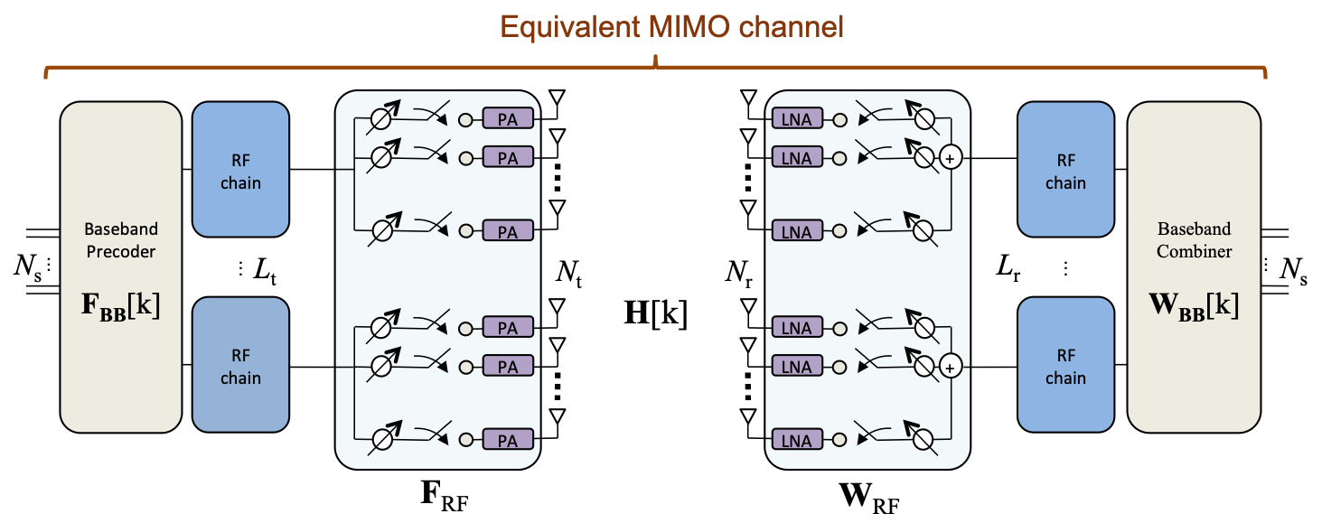
Figure 1: Illustration of the structure of a partially-connected hybrid MIMO architecture, which includes analog and digital precoders and combiners. This figure has been taken from [26].

In this paper, I focus on the problem of estimating the unknown CFO $\Delta f$, PN samples $\theta[n]$, and frequency-selective mmWave MIMO channel $\{{\mathbf{H}}[d]\}_{d=0}^{D-1}$. Given the high dimensionality of the channel matrices, I consider a training protocol in which the transmitter forwards $M$ training frames to the receiver [19], [3], [18], [21], which must estimate the different unknown synchronization parameters. In view of this, for the $m$-th training frame, $1\leq m\leq M$, I set $\bm{\mathsf{F}}^{(m)}[k]=\bm{\mathsf{F}}_{\text{tr}}^{(m)}$, and $\bm{\mathsf{W}}^{(m)}[k]=\bm{\mathsf{W}}_{\text{tr}}^{(m)}$, for every $0\leq k\leq K-1$. Furthermore, I design the training symbols in (1) as ${\bm{\mathsf{s}}}_{t}^{(m)}[k]={\bm{\mathsf{q}}}^{(m)}{\bm{\mathsf{s}}}_{t}^{(m)}[k]$, where ${\bm{\mathsf{q}}}^{(m)}$ operates as an equivalent baseband precoder for this particular design of the training sequence [19]. Therefore, for the transmission of the $m$-th training frame, comprising of $N_{\mathrm{tr}}$ OFDM symbols, the received signal reads as

$${\mathbf{y}}^{(m)}[n]=\bm{\mathsf{W}}_{\text{tr}}^{(m)*}\sum_{d=0}^{D-1}{\mathbf{H}}[d]\bm{\mathsf{F}}_{\text{tr}}^{(m)}{\bm{\mathsf{q}}}^{(m)}s[n-d-n_{0}]e^{{\mathsf{j}}(2\pi\Delta f^{(m)}n+\theta^{(m)}[n])}+{\mathbf{v}}^{(m)}[n],$$ (3)

in which ${\mathbf{v}}^{(m)}[n]\sim{\cal CN}\left(\bm{0},\sigma^{2}\bm{\mathsf{W}}_{\text{tr}}^{(m)*}\bm{\mathsf{W}}_{\text{tr}}^{(m)}\right)$ is the received post-combining circularly-symmetric complex additive Gaussian noise. As shown in [23], [19], the ML criterion establishes that the baseband combiner must whiten the received signal to estimate the different unknown parameters. For this purpose, let us consider the Cholesky decomposition of $\bm{\mathsf{C}}_{\text{w}}^{(m)}=\bm{\mathsf{W}}_{\text{tr}}^{(m)*}\bm{\mathsf{W}}_{\text{tr}}^{(m)}$ as $\bm{\mathsf{C}}_{\text{w}}^{(m)}=\bm{\mathsf{D}}_{\text{w}}^{(m)*}\bm{\mathsf{D}}_{\text{w}}^{(m)}$, with $\bm{\mathsf{D}}_{\text{w}}^{(m)}\in\mathbb{C}^{L_{\mathrm{r}}\times L_{\mathrm{r}}}$ an upper triangular matrix. Now, let us define a vector ${\mathbf{g}}^{(m)}[d]\in\mathbb{C}^{L_{\mathrm{r}}\times 1}$, ${\mathbf{g}}^{(m)}[d]=\bm{\mathsf{D}}_{\text{w}}^{(m)-*}\bm{\mathsf{W}}_{\text{tr}}^{(m)*}{\mathbf{H}}[d]\bm{\mathsf{F}}_{\text{tr}}^{(m)}{\bm{\mathsf{q}}}^{(m)}$, containing the complex equivalent channel samples for a given training step $1\leq m\leq M$. Accordingly, for the $m$-th transmitted frame, the received signal in (3) can be expressed as [26]

$$\begin{split}{\mathbf{y}}^{(m)}[n]&=e^{{\mathsf{j}}(2\pi\Delta f^{(m)}n+\theta^{(m)}[n])}\sum_{d=0}^{D-1}\underbrace{{\mathbf{g}}^{(m)}[d]s^{(m)}[n-d-n_{0}]}_{{\mathbf{x}}^{(m)}[n,d,n_{0}]}\\ &+{\mathbf{v}}^{(m)}[n],\quad n=0,\ldots,n_{0}+(L_{\mathrm{c}}+K)N_{\mathrm{tr}}+D-1\end{split}$$ (4)

with ${\mathbf{v}}^{(m)}[n]\sim{\cal CN}(\bm{0},\sigma^{2}{\mathbf{I}}_{L_{\mathrm{r}}})$ being the post-whitened spatially white received noise vector, and ${\mathbf{g}}^{(m)}[d]=[\alpha_{1}[d]e^{j\beta_{1}[d]},\ldots,\alpha_{L_{\mathrm{r}}}[d]e^{j\beta_{L_{\mathrm{r}}}[d]}]^{T}$ is the complex equivalent beamformed channel for the $m$-th training step and $d$-th delay tap. Therefore, the interest here lies on estimating the vector of parameters $\bm{\xi}^{(m)}\triangleq\left[\left\{{\mathbf{g}}^{(m)T}[d]\right\}_{d=0}^{D-1},\Delta f^{(m)},\{\theta^{(m)}[n]\}_{n=0}^{N+n_{0}+D-1},n_{0},\sigma^{2}\right]^{T}$ for every training frame. In the next section, I theoretically analyze this estimation problem and find the hybrid CRLB for the different parameters in $\bm{\xi}^{(m)}$.

The PN impairment is modeled according to the IEEE 802.11ad wireless standard, whose details are given in [24]. The power spectral density (PSD) of the PN is given in [25], [26], and the reader is referred therein for more details regarding the mathematical model of this parameter.

The discrete-time MIMO channel between the transmitter and the receiver is modeled as a set of $N_{\mathrm{r}}\times N_{\mathrm{t}}$ matrices denoted as ${\mathbf{H}}[d]$, for a given delay tap $d=0,\ldots,D-1$, with $D$ the delay tap length of the channel. Each of the matrices ${\mathbf{H}}[d]$ is assumed to be a sum of the contributions of $C$ spatial clusters, each contributing with $R_{c}$ rays, $c=1,\ldots,C$. I use $\rho_{\mathrm{L}}$ to denote the pathloss, $\alpha_{c,r}\in\mathbb{C}$ is the complex gain of the $r$-th ray within the $c$-th cluster, $\tau_{c,r}\in\mathbb{R}_{+}$ is the time delay of the $r$-th ray within the $c$-th cluster, $\phi_{c,r},\theta_{c,r}\in[0,2\pi)$ are the AoA and AoD, ${\mathbf{a}}_{\mathrm{R}}(\cdot)\in{\mathbb{C}}^{N_{\mathrm{r}}\times 1}$ and ${\mathbf{a}}_{\mathrm{T}}(\cdot)\in{\mathbb{C}}^{N_{\mathrm{t}}\times 1}$ denote the receive and transmit array steering vectors, $p_{\text{RC}}(\tau)$ is the equivalent transmit-receive baseband pulse shape including analog filtering effects evaluated at $\tau$ [27], and $T_{\mathrm{s}}$ is the sampling interval. Using this notation, the frequency-domain channel matrix at the $k$-th subcarrier is given by

$$\begin{split}\bm{\mathsf{H}}[k]&=\sqrt{\frac{N_{\mathrm{r}}N_{\mathrm{t}}}{\rho_{\text{L}}\sum_{c=1}^{C}{R_{c}}}}\sum_{k=0}^{K-1}\sum_{c=1}^{C}\sum_{r=1}^{R_{c}}\alpha_{c,r}p_{\text{RC}}(dT_{\mathrm{s}}-\tau_{c,r})\times\\ &\times{\mathbf{a}}_{\mathrm{R}}\left(\phi_{c,r}\right){\mathbf{a}}_{\mathrm{T}}^{*}(\theta_{c,r})e^{-{\mathsf{j}}\frac{2\pi k}{K}}.\end{split}$$ (5)

Taking the inverse Fourier transform of (5) allows obtaining the discrete-time MIMO channel used in (3). The channel matrix can be represented more compactly as

$$\begin{split}\bm{\mathsf{H}}[k]&=\bm{\mathsf{A}}_{\text{R}}\bm{\mathsf{G}}[k]\bm{\mathsf{A}}_{\text{T}}^{*},\end{split}$$ (6)

where $\bm{\mathsf{G}}[k]\in\mathbb{C}^{\sum_{c=1}^{C}{R_{c}}\times\sum_{c=1}^{C}{R_{c}}}$ is a diagonal matrix containing the path gains and the equivalent pulse-shaping effect, and $\bm{\mathsf{A}}_{\text{T}}\in\mathbb{C}^{N_{\mathrm{t}}\times\sum_{c=1}^{C}R_{c}}$, $\bm{\mathsf{A}}_{\text{R}}\in\mathbb{C}^{N_{\mathrm{r}}\times\sum_{c=1}^{C}R_{c}}$ are the frequency-selective array response matrices evaluated on the AoD and AoA, respectively. Finally, the matrix $\bm{\mathsf{H}}[k]$ in (6) can be approximated using the extended virtual channel model [28] as

$$\bm{\mathsf{H}}[k]\approx\tilde{\bm{\mathsf{A}}}_{\text{R}}\bm{\mathsf{G}}^{\text{v}}[k]\tilde{\bm{\mathsf{A}}}_{\text{T}}^{*},$$ (7)

where $\bm{\mathsf{G}}^{\text{v}}[k]\in\mathbb{C}^{G_{\mathrm{r}}\times G_{\mathrm{t}}}$ is a sparse matrix containing the path gains of the quantized spatial frequencies in the non-zero elements, and the dictionary matrices $\tilde{\bm{\mathsf{A}}}_{\text{T}}\in\mathbb{C}^{N_{\mathrm{t}}\times G_{\mathrm{t}}}$, $\tilde{\bm{\mathsf{A}}}_{\text{R}}\in\mathbb{C}^{N_{\mathrm{r}}\times G_{\mathrm{r}}}$ contain the transmit and receive array response vectors evaluated on spatial grids of sizes $G_{\mathrm{t}}$ and $G_{\mathrm{r}}$, respectively.

IV Theoretical analysis of the estimation problem

In this section, I theoretically analyze the problem of estimating the unknown parameters in $\bm{\xi}^{(m)}$. Let us assume, without loss of generality, that $N_{\mathrm{tr}}$ OFDM symbols are transmitted for the $m$-th training frame, and that the number of available received time-domain samples of ${\mathbf{r}}^{(m)}[n]$ is given by $N=n_{0}+(L_{\mathrm{c}}+K)N_{\mathrm{tr}}+D$. Assuming that the received time-domain noise samples in (4) are independent and identically distributed, the received signal in (4) has log-likelihood function (LLF) given by

$$\begin{split}&\log{p\left(\{{\mathbf{r}}^{(m)}[n]\}_{n=0}^{N-1};\bm{\xi}^{(m)}\right)}=-N\log{(\pi\sigma^{2})}-\frac{1}{\sigma^{2}}\sum_{n=0}^{N-1}\left\|{\mathbf{r}}^{(m)}[n]\right\|_{2}^{2}\\ &+2\sum_{n=0}^{N-1}\mathop{\mathrm{Re}}\left\{{\mathbf{r}}^{(m)*}e^{{\mathsf{j}}(2\pi\Delta f^{(m)}n+\theta^{(m)}[n])}\sum_{d=0}^{D-1}{\mathbf{x}}^{(m)}[n,d,n_{0}]\right\}-\sum_{n=0}^{N-1}\left\|\sum_{d=0}^{D-1}{\mathbf{x}}^{(m)}[n,d,n_{0}]\right\|_{2}^{2}.\end{split}$$ (8)

To ensure robustness of the synchronization algorithm, I will focus on finding the ML estimators for the different unknown parameters in $\bm{\xi}^{(m)}$. From (8), it is observed that maximizing ${\cal L}(\bm{\xi}^{(m)})=\log{p\left(\{{\mathbf{r}}^{(m)}[n]\}_{n=0}^{N-1};\bm{\xi}^{(m)}\right)}$ as a function of $n_{0}$ requires knowledge of the other parameters contained in $\bm{\xi}^{(m)}$, which suggests that the ML estimator exhibits high computational complexity. To reduce computational complexity, I propose to exploit the good correlation properties of Golay sequences [12], [29], and append a $64$-point $G_{\text{a},64}$ sequence at the beginning of the training frame, which has been shown to offer excellent performance in the absence of PN [30]. Thereby, a practical TO estimator can be devised by maximizing the third term in (8), which is given by [30, 2]

$$\begin{split}\hat{n}_{0}&=\underset{n_{0}}{\arg\,\max}\sum_{i=1}^{L_{\mathrm{r}}}\sum_{n=0}^{63}\left|r_{i}^{(m)*}[n]s^{(m)}[n-d-n_{0}]\right|,\end{split}$$ (9)

which explicitly exploits the information coming from having $L_{\mathrm{r}}\geq 1$ at the receiver side. Assuming that the TO has been estimated perfectly using (9), this parameter can be compensated by advancing the receive signal by $\hat{n}_{0}$ as ${\mathbf{r}}^{(m)}[n]={\mathbf{y}}^{(m)}[n+n_{0}]$, $n=0,\ldots,(L_{\mathrm{c}}+K)N_{\mathrm{tr}}+D-1$. Now, let the initial sample of the $t$-th OFDM symbol after CP removal be defined as $k_{0}[t]\triangleq L_{\mathrm{c}}+n_{0}+t(K+L_{\mathrm{c}})$, let $\phi^{(m)}[n_{0},t]\triangleq e^{{\mathsf{j}}2\pi\Delta f^{(m)}k_{0}[t]}$ be the common phase change at the $t$-th OFDM symbol due to TO, let $\bm{\Omega}_{t}\left(\Delta f^{(m)}\right)\triangleq\phi^{(m)}[n_{0},t]\bigoplus_{n=0}^{K-1}e^{{\mathsf{j}}2\pi\Delta f^{(m)}n}$ be the CFO matrix impairing the $t$-th OFDM symbol, and let $\bm{\mathsf{S}}_{t}^{(m)}\triangleq\bigoplus_{k=0}^{K-1}{\mathsf{s}}_{t}^{(m)}[k]$ and $\bm{\mathsf{S}}^{(m)}\triangleq\left[\begin{array}[]{ccc}\bm{\mathsf{S}}_{0}^{(m)T}&\ldots&\bm{\mathsf{S}}_{N_{\mathrm{tr}}}^{(m)T}\\ \end{array}\right]^{T}$ be matrices containing the $t$-th OFDM training symbol and the $N_{\mathrm{tr}}$ OFDM training symbols, respectively. Also, let ${\bm{\mathsf{g}}}_{i}^{(m)}\triangleq\left[\begin{array}[]{ccc}{\mathsf{g}}_{i}^{(m)}[0]&\ldots&{\mathsf{g}}_{i}^{(m)}[K-1]\\ \end{array}\right]$ be the frequency-response of the equivalent beamformed channel seen by the $i$-th receive RF chain, let ${\mathbf{v}}_{i,t}^{(m)}\triangleq\left[\begin{array}[]{ccc}v_{i}^{(m)}[k_{0}[t]]&\ldots&v_{i}^{(m)}[k_{0}[t]+K-1]\\ \end{array}\right]$ contain the time-domain noise samples impairing the $t$-th OFDM symbol, let $\bm{\theta}_{t}^{(m)}=\left[\begin{array}[]{ccc}\theta^{(m)}[k_{0}[t]]&\ldots&\theta^{(m)}[k_{0}[t]+K-1]\\ \end{array}\right]^{T}$ be the PN vector corresponding to the $t$-th OFDM symbol, and let ${\mathbf{P}}\left(\bm{\theta}_{t}^{(m)}\right)\triangleq\bigoplus_{n=0}^{K-1}e^{{\mathsf{j}}\theta^{(m)}[k_{0}[t]+n]}$ be the diagonal PN matrix impairing the received $t$-th OFDM symbol. Letting ${\mathbf{F}}\in\mathbb{C}^{K\times K}$ denote the $K$-point DFT matrix, the received time synchronized signal ${\mathbf{r}}^{(m)}[n]$ can be vectorized as

$$\begin{split}\underbrace{\left[\begin{array}[]{c}r_{i}^{(m)}[k_{0}[t]]\\ \vdots\\ r_{i}^{(m)}[k_{0}[t]+K-1]\\ \end{array}\right]}_{{\mathbf{r}}_{i,t}^{(m)}}&=\bm{\Omega}_{t}\left(\Delta f^{(m)}\right){\mathbf{P}}_{t}\left(\bm{\theta}_{t}^{(m)}\right)\underbrace{\frac{1}{\sqrt{K}}\left[\begin{array}[]{ccc}e^{{\mathsf{j}}\frac{2\pi 0}{K}}&\ldots&e^{{\mathsf{j}}\frac{2\pi 0(K-1)}{K}}\\ \vdots&\ddots&\vdots\\ e^{{\mathsf{j}}\frac{2\pi 0(K-1)}{K}}&\ldots&e^{{\mathsf{j}}\frac{2\pi(K-1)(K-1)}{K}}\\ \end{array}\right]}_{{\mathbf{F}}^{*}}\\ &\times\underbrace{\left(\bigoplus_{k=0}^{K-1}{\mathsf{s}}_{t}^{(m)}[k]\right)}_{\bm{\mathsf{S}}_{t}^{(m)}}\underbrace{\left[\begin{array}[]{c}{\mathsf{g}}_{i}^{(m)}[0]\\ \vdots\\ {\mathsf{g}}_{i}^{(m)}[K-1]\\ \end{array}\right]}_{{\bm{\mathsf{g}}}_{i}^{(m)}}+\underbrace{\left[\begin{array}[]{c}v_{i}^{(m)}[k_{0}[t]]\\ \vdots\\ v_{i}^{(m)}[k_{0}[t]+K-1]\\ \end{array}\right]}_{{\mathbf{v}}_{i,t}^{(m)}},\end{split}$$ (10)

such that the vectorized received signal can be simplified as

$${\mathbf{r}}_{i,t}^{(m)}=\bm{\Omega}_{t}\left(\Delta f^{(m)}\right){\mathbf{P}}_{t}\left(\bm{\theta}_{t}^{(m)}\right){\mathbf{F}}^{*}\bm{\mathsf{S}}_{t}^{(m)}{\bm{\mathsf{g}}}_{i}^{(m)}+{\mathbf{v}}_{i,t}^{(m)}.$$ (11)

Now, the $K\times 1$ random vector ${\mathbf{r}}_{i,t}^{(m)}$ can be stacked for the different received OFDM symbols $1\leq t\leq N_{\mathrm{tr}}$ and RF chains $1\leq i\leq L_{\mathrm{r}}$ as

$$\begin{split}\underbrace{\left[\begin{array}[]{c}{\mathbf{r}}_{i,1}^{(m)}\\ \vdots\\ {\mathbf{r}}_{i,N_{\mathrm{tr}}}^{(m)}\\ \end{array}\right]}_{{\mathbf{r}}_{i}^{(m)}}&=\underbrace{\left(\bigoplus_{t=1}^{N_{\mathrm{tr}}}\bm{\Omega}_{t}\left(\Delta f^{(m)}\right)\right)}_{\bm{\Omega}\left(\Delta f^{(m)}\right)}\underbrace{\left(\bigoplus_{t=1}^{N_{\mathrm{tr}}}{\mathbf{P}}_{t}\left(\bm{\theta}_{t}^{(m)}\right)\right)}_{{\mathbf{P}}\left(\bm{\theta}^{(m)}\right)}\underbrace{\left({\mathbf{I}}_{N_{\mathrm{tr}}}\otimes{\mathbf{F}}^{*}\right)}_{{\mathbf{F}}_{\otimes}^{*}}\\ &\times\underbrace{\left[\begin{array}[]{c}\bm{\mathsf{S}}_{1}^{(m)}\\ \vdots\\ \bm{\mathsf{S}}_{N_{\mathrm{tr}}}^{(m)}\\ \end{array}\right]}_{\bm{\mathsf{S}}^{(m)}}{\bm{\mathsf{g}}}_{i}^{(m)}+\underbrace{\left[\begin{array}[]{c}{\mathbf{v}}_{i,1}^{(m)}\\ \vdots\\ {\mathbf{v}}_{i,N_{\mathrm{tr}}}^{(m)}\\ \end{array}\right]}_{{\mathbf{v}}_{i}^{(m)}}.\end{split}$$ (12)

Therefore, the received signal ${\mathbf{r}}_{i}^{(m)}$ is distributed according to ${\cal CN}\left(\bm{\mu}_{i}^{(m)}\left(\bm{\xi}^{(m)}\right),\sigma^{2}{\mathbf{I}}_{KN_{\mathrm{tr}}}\right)$, where $\bm{\mu}_{i}^{(m)}\left(\bm{\xi}^{(m)}\right)=\bm{\Omega}\left(\Delta f^{(m)}\right){\mathbf{P}}\left(\bm{\theta}^{(m)}\right){\mathbf{F}}_{\otimes}^{*}\bm{\mathsf{S}}^{(m)}{\bm{\mathsf{g}}}_{i}^{(m)}$. Finally, stacking the received signals ${\mathbf{r}}_{i}^{(m)}$ for the different RF chains yields

$$\left[\begin{array}[]{c}{\mathbf{r}}_{1}^{(m)}\\ \vdots\\ {\mathbf{r}}_{L_{\mathrm{r}}}^{(m)}\\ \end{array}\right]=\left({\mathbf{I}}_{L_{\mathrm{r}}}\otimes\bm{\Omega}\left(\Delta f^{(m)}\right){\mathbf{P}}\left(\bm{\theta}^{(m)}\right){\mathbf{F}}_{\otimes}^{*}\bm{\mathsf{S}}^{(m)}\right)\left[\begin{array}[]{c}{\bm{\mathsf{g}}}_{1}^{(m)}\\ \vdots\\ {\bm{\mathsf{g}}}_{L_{\mathrm{r}}}^{(m)}\\ \end{array}\right]+\left[\begin{array}[]{c}{\mathbf{v}}_{1}^{(m)}\\ \vdots\\ {\mathbf{v}}_{L_{\mathrm{r}}}^{(m)}\\ \end{array}\right].$$ (13)

For the purpose of theoretically analyzing the estimation problem of finding the unknown parameters, let ${\mathsf{g}}_{i}^{(m)}[k]$ be further expressed as ${\mathsf{g}}_{i}^{(m)}[k]=\alpha_{i}^{(m)}[k]e^{{\mathsf{j}}\beta_{i}^{(m)}[k]}$, and let $\tilde{{\bm{\mathsf{g}}}}_{i}^{(m)}[k]\in\mathbb{C}^{2}$ be defined as $\tilde{{\bm{\mathsf{g}}}}_{i}^{(m)}[k]\triangleq[\alpha_{i}^{(m)}[k],\beta_{i}^{(m)}[k]]^{T}$. Finally, let $\tilde{{\bm{\mathsf{g}}}}_{i}^{(m)}\in\mathbb{C}^{2K\times 1}$ be given by $\tilde{{\bm{\mathsf{g}}}}_{i}^{(m)}\triangleq[\tilde{{\bm{\mathsf{g}}}}_{i}^{(m)T}[0],\ldots,\tilde{{\bm{\mathsf{g}}}}_{i}^{(m)T}[K-1]]^{T}$, and $\tilde{{\bm{\mathsf{g}}}}^{(m)}\triangleq[\tilde{{\bm{\mathsf{g}}}}_{1}^{(m)T},\ldots,\tilde{{\bm{\mathsf{g}}}}_{L_{\mathrm{r}}}^{(m)T}]^{T}$. Likewise, let $\bm{\theta}^{(m)}\triangleq[\bm{\theta}_{0}^{(m)T},\ldots,\bm{\theta}_{N_{\mathrm{tr}}-1}^{(m)T}]T$. Now, the vector of parameters to be estimated is defined as $\bm{\xi}^{(m)}\in\mathbb{C}^{(K(L_{\mathrm{r}}+N_{\mathrm{tr}})+1)\times 1}$, given by $\bm{\xi}^{(m)}\triangleq[\Delta f^{(m)},\tilde{{\bm{\mathsf{g}}}}^{(m)T},\bm{\theta}^{(m)T}]^{T}$.

IV-A Computation of the hybrid information matrix (HIM)

In this section, I derive the HIM of the vector of parameters $\bm{\xi}^{(m)}$ and derive the hybrid CRLB for any unbiased estimator of $\bm{\xi}^{(m)}$. Since there is prior knowledge on the PN parameters in $\bm{\theta}_{t}^{(m)}$, $0\leq t\leq N_{\mathrm{tr}}$, the HIM ${\mathbf{H}}\left(\bm{\xi}^{(m)}\right)$ can be defined as [31]

$${\mathbf{H}}\left(\bm{\xi}^{(m)}\right)={\mathbf{I}}_{\text{D}}\left(\bm{\xi}^{(m)}\right)+{\mathbf{I}}_{\text{P}}\left(\bm{\xi}^{(m)}\right),$$ (14)

where

$${\mathbf{I}}_{\text{D}}\left(\bm{\xi}^{(m)}\right)\triangleq\mathbb{E}_{\bm{\theta}^{(m)}}\left\{{\mathbf{I}}\left(\bm{\xi}^{(m)}\right)\right\},$$ (15)

with ${\mathbf{I}}\left(\bm{\xi}^{(m)}\right)$ denoting the Fisher information matrix (FIM) and

$${\mathbf{I}}_{\text{P}}\left(\bm{\xi}^{(m)}\right)\triangleq-\mathbb{E}_{\bm{\theta}^{(m)}|\tilde{{\bm{\mathsf{g}}}}^{(m)},\Delta f^{(m)}}\left\{\frac{\partial^{2}\log{p\left(\bm{\theta}^{(m)}|\tilde{{\bm{\mathsf{g}}}}^{(m)},\Delta f^{(m)}\right)}}{\partial\bm{\xi}^{(m)}\bm{\xi}^{(m)T}}\right\}$$ (16)

is the prior information matrix with $p\left(\bm{\theta}^{(m)}|\tilde{{\bm{\mathsf{g}}}}^{(m)},\Delta f^{(m)}\right)$ denoting the prior distribution of the PN vector given the equivalent beamformed channels $\tilde{{\bm{\mathsf{g}}}}^{(m)}$ and the CFO $\Delta f^{(m)}$.

The FIM associated to $\bm{\xi}^{(m)}$, ${\mathbf{I}}\left(\bm{\xi}^{(m)}\right)\in\mathbb{R}^{(K(L_{\mathrm{r}}+N_{\mathrm{tr}})+1)\times(K(L_{\mathrm{r}}+N_{\mathrm{tr}})+1)}$, can be expressed as [32]

$$[{\mathbf{I}}\left(\bm{\xi}^{(m)}\right)]_{r,c}=\frac{2}{\sigma^{2}}\sum_{i=1}^{L_{\mathrm{r}}}\mathop{\mathrm{Re}}\left\{\frac{\partial\bm{\mu}_{i}^{(m)*}\left(\bm{\xi}^{(m)}\right)}{\partial\xi_{r}^{(m)}}\frac{\partial\bm{\mu}_{i}^{(m)}\left(\bm{\xi}^{(m)}\right)}{\partial\xi_{c}^{(m)}}\right\},\quad 1\leq r,c\leq K(L_{\mathrm{r}}+N_{\mathrm{tr}})+1.$$ (17)

Let ${\mathbf{e}}_{m}^{n}\in\mathbb{R}^{n}$ denote the $m$-th canonical vector in $\mathbb{R}^{n}$, and let $p[t,\ell]=n_{0}+L_{\mathrm{c}}+(t-1)(K+L_{\mathrm{c}})+\ell$. Then, the terms $\frac{\partial\bm{\mu}_{i}^{(m)}\left(\bm{\xi}^{(m)}\right)}{\partial\xi_{r}^{(m)}}$ are given by

$$\begin{split}\frac{\partial\bm{\mu}_{i}^{(m)}\left(\bm{\xi}^{(m)}\right)}{\partial\xi_{r}^{(m)}}=\left\{\begin{array}[]{cc}{\mathsf{j}}{\mathbf{M}}\bm{\Omega}\left(\Delta f^{(m)}\right){\mathbf{P}}\left(\bm{\theta}^{(m)}\right){\mathbf{F}}_{\otimes}^{*}\bm{\mathsf{S}}^{(m)}{\bm{\mathsf{g}}}_{i}^{(m)}&\xi_{r}^{(m)}=\Delta f^{(m)}\\ {\mathsf{j}}\mathop{\mathrm{diag}}\left\{\bm{\Omega}\left(\Delta f^{(m)}\right){\mathbf{F}}_{\otimes}^{*}\bm{\mathsf{S}}^{(m)}{\bm{\mathsf{g}}}_{i}^{(m)}\right\}e^{{\mathsf{j}}\theta_{t}^{(m)}[\ell]}{\mathbf{e}}_{p[t,\ell]}^{KN_{\mathrm{tr}}}&\xi_{r}^{(m)}=\theta_{t}^{(m)}[\ell]\\ e^{{\mathsf{j}}\beta_{i}^{(m)}[k]}\bm{\Omega}\left(\Delta f^{(m)}\right){\mathbf{P}}\left(\bm{\theta}^{(m)}\right){\mathbf{F}}_{\otimes}^{*}\bm{\mathsf{S}}^{(m)}{\mathbf{e}}_{k}^{K}&\xi_{r}^{(m)}=\alpha_{i}^{(m)}[k]\\ {\mathsf{j}}{\mathsf{g}}_{i}^{(m)}[k]\bm{\Omega}\left(\Delta f^{(m)}\right){\mathbf{P}}\left(\bm{\theta}^{(m)}\right){\mathbf{F}}_{\otimes}^{*}\bm{\mathsf{S}}^{(m)}{\mathbf{e}}_{k}^{K}&\xi_{r}^{(m)}=\beta_{i}^{(m)}[k].\\ \end{array}\right.\end{split}$$ (18)

where ${\mathbf{M}}\in\mathbb{C}^{K\times K}$ is given by ${\mathbf{M}}\triangleq\bigoplus_{t=0}^{N_{\mathrm{tr}}-1}{\mathbf{M}}[t]$, with ${\mathbf{M}}[t]$ given by ${\mathbf{M}}[t]=2\pi\bigoplus_{n=0}^{K-1}(k_{0}[t]+n)$. The FIM can be structured as

$${\mathbf{I}}\left(\bm{\xi}^{(m)}\right)=\frac{2}{\sigma^{2}}\mathop{\mathrm{Re}}\left\{\left[\begin{array}[]{ccccccc}i_{\Delta f^{(m)},\Delta f^{(m)}}\left(\bm{\xi}^{(m)}\right)&{\mathbf{i}}_{\Delta f^{(m)},\tilde{{\bm{\mathsf{g}}}}^{(m)}}\left(\bm{\xi}^{(m)}\right)&{\mathbf{i}}_{\Delta f^{(m)},\bm{\theta}^{(m)}}\left(\bm{\xi}^{(m)}\right)\\ {\mathbf{i}}_{\tilde{{\bm{\mathsf{g}}}}^{(m)},\Delta f^{(m)}}\left(\bm{\xi}^{(m)}\right)&{\mathbf{I}}_{\tilde{{\bm{\mathsf{g}}}}^{(m)},\tilde{{\bm{\mathsf{g}}}}^{(m)}}\left(\bm{\xi}^{(m)}\right)&{\mathbf{I}}_{\tilde{{\bm{\mathsf{g}}}}^{(m)},\bm{\theta}^{(m)}}\left(\bm{\xi}^{(m)}\right)\\ {\mathbf{i}}_{\bm{\theta}^{(m)},\Delta f^{(m)}}\left(\bm{\xi}^{(m)}\right)&{\mathbf{I}}_{\bm{\theta}^{(m)},\tilde{{\bm{\mathsf{g}}}}^{(m)}}\left(\bm{\xi}^{(m)}\right)&{\mathbf{I}}_{\bm{\theta}^{(m)},\bm{\theta}^{(m)}}\left(\bm{\xi}^{(m)}\right)\\ \end{array}\right]\right\}.$$ (19)

The element $i_{\Delta f^{(m)},\Delta f^{(m)}}\left(\bm{\xi}^{(m)}\right)$ is given by

$$\begin{split}i_{\Delta f^{(m)},\Delta f^{(m)}}\left(\bm{\xi}^{(m)}\right)&=\sum_{i=1}^{L_{\mathrm{r}}}{\bm{\mathsf{g}}}_{i}^{(m)*}\bm{\mathsf{S}}^{(m)*}{\mathbf{F}}_{\otimes}{\mathbf{M}}^{*}{\mathbf{M}}{\mathbf{F}}_{\otimes}^{*}\bm{\mathsf{S}}^{(m)}{\bm{\mathsf{g}}}_{i}^{(m)}\\ &=\sum_{i=1}^{L_{\mathrm{r}}}\sum_{t=0}^{N_{\mathrm{tr}}-1}{\bm{\mathsf{g}}}_{i}^{(m)*}\bm{\mathsf{S}}_{t}^{(m)*}{\mathbf{F}}{\mathbf{M}}^{*}[t]{\mathbf{M}}[t]{\mathbf{F}}^{*}\bm{\mathsf{S}}_{t}^{(m)}{\bm{\mathsf{g}}}_{i}^{(m)}.\end{split}$$ (20)

The vector ${\mathbf{i}}_{\Delta f^{(m)},\tilde{{\bm{\mathsf{g}}}}^{(m)}}\left(\bm{\xi}^{(m)}\right)$ can be expressed as

$${\mathbf{i}}_{\Delta f^{(m)},\tilde{{\bm{\mathsf{g}}}}^{(m)}}\left(\bm{\xi}^{(m)}\right)=\left[\begin{array}[]{ccc}{\mathbf{i}}_{\Delta f^{(m)},\tilde{{\bm{\mathsf{g}}}}_{1}^{(m)}}\left(\bm{\xi}^{(m)}\right)&\ldots&{\mathbf{i}}_{\Delta f^{(m)},\tilde{{\bm{\mathsf{g}}}}_{L_{\mathrm{r}}}^{(m)}}\left(\bm{\xi}^{(m)}\right)\\ \end{array}\right],$$ (21)

with ${\mathbf{i}}_{\Delta f^{(m)},\tilde{{\bm{\mathsf{g}}}}_{i}^{(m)}}\left(\bm{\xi}^{(m)}\right)$, $1\leq i\leq L_{\mathrm{r}}$, being given by

$${\mathbf{i}}_{\Delta f^{(m)},\tilde{{\bm{\mathsf{g}}}}_{i}^{(m)}}\left(\bm{\xi}^{(m)}\right)=\left[\begin{array}[]{ccc}{\mathbf{i}}_{\Delta f^{(m)},\tilde{{\bm{\mathsf{g}}}}_{i}^{(m)}[0]}\left(\bm{\xi}^{(m)}\right)&\ldots&{\mathbf{i}}_{\Delta f^{(m)},\tilde{{\bm{\mathsf{g}}}}_{i}^{(m)}[K-1]}\left(\bm{\xi}^{(m)}\right)\\ \end{array}\right],$$ (22)

and the vector ${\mathbf{i}}_{\Delta f^{(m)},\tilde{{\bm{\mathsf{g}}}}_{i}^{(m)}[k]}\left(\bm{\xi}^{(m)}\right)$, $0\leq k\leq K-1$, is given by

$$\begin{split}{\mathbf{i}}_{\Delta f^{(m)},\tilde{{\bm{\mathsf{g}}}}_{i}^{(m)}[k]}\left(\bm{\xi}^{(m)}\right)&=\left[\begin{array}[]{ccc}i_{\Delta f^{(m)},\alpha_{i}^{(m)}[k]}\left(\bm{\xi}^{(m)}\right)&i_{\Delta f^{(m)},\beta_{i}^{(m)}[k]}\left(\bm{\xi}^{(m)}\right)\\ \end{array}\right]\\ &=\sum_{t=0}^{N_{\mathrm{tr}}-1}\left[\begin{array}[]{cc}-{\mathsf{j}}e^{{\mathsf{j}}\beta_{i}^{(m)}[k]}&{\mathsf{g}}_{i}^{(m)}[k]\\ \end{array}\right]{\bm{\mathsf{g}}}_{i}^{(m)*}\bm{\mathsf{S}}_{t}^{(m)*}{\mathbf{F}}{\mathbf{M}}[t]{\mathbf{F}}^{*}\bm{\mathsf{S}}_{t}^{(m)}{\mathbf{e}}_{k}^{K}.\end{split}$$ (23)

Furthermore, the vector ${\mathbf{i}}_{\Delta f^{(m)},\bm{\theta}^{(m)}}\left(\bm{\xi}^{(m)}\right)$ can be written as

$${\mathbf{I}}_{\Delta f^{(m)},\bm{\theta}^{(m)}}\left(\bm{\xi}^{(m)}\right)=\left[\begin{array}[]{ccc}{\mathbf{I}}_{\Delta f^{(m)},\bm{\theta}_{0}^{(m)}}\left(\bm{\xi}^{(m)}\right)&\ldots&{\mathbf{I}}_{\Delta f^{(m)},\bm{\theta}_{N_{\mathrm{tr}}-1}^{(m)}}\left(\bm{\xi}^{(m)}\right)\\ \end{array}\right],$$ (24)

where ${\mathbf{i}}_{\Delta f^{(m)},\bm{\theta}_{t}^{(m)}}\left(\bm{\xi}^{(m)}\right)$, $0\leq t\leq N_{\mathrm{tr}}-1$, is given by

$${\mathbf{i}}_{\Delta f^{(m)},\bm{\theta}_{t}^{(m)}}\left(\bm{\xi}^{(m)}\right)=\left[\begin{array}[]{ccc}i_{\Delta f^{(m)},\theta_{t}^{(m)}[0]}\left(\bm{\xi}^{(m)}\right)&\ldots&i_{\Delta f^{(m)},\theta_{t}^{(m)}[K-1]}\left(\bm{\xi}^{(m)}\right)\\ \end{array}\right].$$ (25)

Each of the terms in (25) can be expressed as

$$i_{\Delta f^{(m)},\theta_{t}^{(m)}[\ell]}\left(\bm{\xi}^{(m)}\right)=\sum_{i=1}^{L_{\mathrm{r}}}{\bm{\mathsf{g}}}_{i}^{(m)*}\bm{\mathsf{S}}_{t}^{(m)*}{\mathbf{F}}{\mathbf{M}}[t]\mathop{\mathrm{diag}}\left\{{\mathbf{F}}^{*}\bm{\mathsf{S}}_{t}^{(m)}{\bm{\mathsf{g}}}_{i}^{(m)}\right\}{\mathbf{e}}_{\ell}^{K}.$$ (26)

The submatrix ${\mathbf{I}}_{\tilde{{\bm{\mathsf{g}}}}^{(m)},\tilde{{\bm{\mathsf{g}}}}^{(m)}}\left(\bm{\xi}^{(m)}\right)$ can be expressed as

$${\mathbf{I}}_{\tilde{{\bm{\mathsf{g}}}}^{(m)},\tilde{{\bm{\mathsf{g}}}}^{(m)}}\left(\bm{\xi}^{(m)}\right)=\left[\begin{array}[]{ccc}{\mathbf{I}}_{\tilde{{\bm{\mathsf{g}}}}_{1}^{(m)},\tilde{{\bm{\mathsf{g}}}}_{L_{\mathrm{r}}}^{(m)}}\left(\bm{\xi}^{(m)}\right)&\ldots&{\mathbf{I}}_{\tilde{{\bm{\mathsf{g}}}}_{1}^{(m)},\tilde{{\bm{\mathsf{g}}}}_{L_{\mathrm{r}}}^{(m)}}\left(\bm{\xi}^{(m)}\right)\\ \vdots&\ddots&\vdots\\ {\mathbf{I}}_{\tilde{{\bm{\mathsf{g}}}}_{L_{\mathrm{r}}}^{(m)},\tilde{{\bm{\mathsf{g}}}}_{1}^{(m)}}\left(\bm{\xi}^{(m)}\right)&\ldots&{\mathbf{I}}_{\tilde{{\bm{\mathsf{g}}}}_{L_{\mathrm{r}}}^{(m)},\tilde{{\bm{\mathsf{g}}}}_{L_{\mathrm{r}}}^{(m)}}\left(\bm{\xi}^{(m)}\right)\\ \end{array}\right],$$ (27)

which has a particularly interesting structure from an estimation theoretic perspective. By observing the Kronecker structure in (13), as well as the derivatives in (18), it is clear that ${\mathbf{I}}_{\tilde{{\bm{\mathsf{g}}}}_{i}^{(m)},\tilde{{\bm{\mathsf{g}}}}_{j}^{(m)}}\left(\bm{\xi}^{(m)}\right)=\bm{0}$ for $i\neq j$. Therefore, only the terms ${\mathbf{I}}_{\tilde{{\bm{\mathsf{g}}}}_{i}^{(m)},\tilde{{\bm{\mathsf{g}}}}_{i}^{(m)}}\left(\bm{\xi}^{(m)}\right)$ are non-zero valued, which can be computed as

$${\mathbf{I}}_{\tilde{{\bm{\mathsf{g}}}}_{i}^{(m)},\tilde{{\bm{\mathsf{g}}}}_{i}^{(m)}}\left(\bm{\xi}^{(m)}\right)=\left[\begin{array}[]{ccc}{\mathbf{I}}_{\tilde{{\bm{\mathsf{g}}}}_{i}^{(m)}[0],\tilde{{\bm{\mathsf{g}}}}_{i}^{(m)}[0]}\left(\bm{\xi}^{(m)}\right)&\ldots&{\mathbf{I}}_{\tilde{{\bm{\mathsf{g}}}}i^{(m)}[0],\tilde{{\bm{\mathsf{g}}}}_{i}^{(m)}[K-1]}\left(\bm{\xi}^{(m)}\right)\\ \vdots&\ddots&\vdots\\ {\mathbf{I}}_{\tilde{{\bm{\mathsf{g}}}}_{i}^{(m)}[K-1],\tilde{{\bm{\mathsf{g}}}}_{i}^{(m)}[0]}\left(\bm{\xi}^{(m)}\right)&\ldots&{\mathbf{I}}_{\tilde{{\bm{\mathsf{g}}}}_{i}^{(m)}[K-1],\tilde{{\bm{\mathsf{g}}}}^{(m)}[K-1]}\left(\bm{\xi}^{(m)}\right)\\ \end{array}\right].$$ (28)

The matrix in (28) has a similar structure to that of (27). From (18) and (12), it is observed that ${\mathbf{I}}_{\tilde{{\bm{\mathsf{g}}}}_{i}^{(m)}[k_{1}],\tilde{{\bm{\mathsf{g}}}}_{i}^{(m)}[k_{2}]}\left(\bm{\xi}^{(m)}\right)=\bm{0}$ if $k_{1}\neq k_{2}$. The non-zero matrices ${\mathbf{I}}_{\tilde{{\bm{\mathsf{g}}}}_{i}^{(m)}[k],\tilde{{\bm{\mathsf{g}}}}_{i}^{(m)}[k]}\left(\bm{\xi}^{(m)}\right)$ can be written as

$${\mathbf{I}}_{\tilde{{\bm{\mathsf{g}}}}_{i}^{(m)}[k],\tilde{{\bm{\mathsf{g}}}}_{i}^{(m)}[k]}\left(\bm{\xi}^{(m)}\right)=\left[\begin{array}[]{cc}{\mathbf{I}}_{\alpha_{i}^{(m)}[k],\alpha_{i}^{(m)}[k]}\left(\bm{\xi}^{(m)}\right)&{\mathbf{I}}_{\alpha_{i}^{(m)}[k],\beta_{i}^{(m)}[k]}\left(\bm{\xi}^{(m)}\right)\\ {\mathbf{I}}_{\beta_{i}^{(m)}[k],\alpha_{i}^{(m)}[k]}\left(\bm{\xi}^{(m)}\right)&{\mathbf{I}}_{\beta_{i}^{(m)}[k],\beta_{i}^{(m)}[k]}\left(\bm{\xi}^{(m)}\right)\\ \end{array}\right].$$ (29)

By plugging the corresponding partial derivatives in (18) into (17), the matrix in (29) is given by

$${\mathbf{I}}_{\tilde{{\bm{\mathsf{g}}}}_{i}^{(m)}[k],\tilde{{\bm{\mathsf{g}}}}_{i}^{(m)}[k]}\left(\bm{\xi}^{(m)}\right)=\sum_{t=0}^{N_{\mathrm{tr}}-1}\left|[\bm{\mathsf{S}}_{t}^{(m)}]_{k,k}\right|^{2}\underbrace{\left[\begin{array}[]{cc}1&0\\ 0&\alpha_{i}^{(m)2}[k]\\ \end{array}\right]}_{\bm{\Lambda}_{i}^{(m)}[k]},$$ (30)

which shows that estimation of both the amplitude and phase of a given subchannel ${\mathsf{g}}_{i}^{(m)}[k]$ do not interfere with each other, a result that has been shown in [19]. Let ${\bm{\mathsf{s}}}_{k}^{(m)}\in\mathbb{C}^{N_{\mathrm{tr}}\times 1}$ be the vector containing the training pilots for a given subcarrier and all the transmitted OFDM symbols, ${\bm{\mathsf{s}}}_{k}^{(m)}=[{\mathsf{s}}_{0}^{(m)}[k],\ldots,{\mathsf{s}}_{N_{\mathrm{tr}}-1}^{(m)}[k]]^{T}$. Then, the matrix in (28) can be expressed as

$${\mathbf{I}}_{\tilde{{\bm{\mathsf{g}}}}_{i}^{(m)},\tilde{{\bm{\mathsf{g}}}}_{i}^{(m)}}\left(\bm{\xi}^{(m)}\right)=\bigoplus_{k=0}^{K-1}\left\|{\bm{\mathsf{s}}}_{k}^{(m)}\right\|_{2}^{2}\bm{\Lambda}_{i}^{(m)}[k],$$ (31)

and (27) can be written as

$${\mathbf{I}}_{\tilde{{\bm{\mathsf{g}}}}^{(m)},\tilde{{\bm{\mathsf{g}}}}^{(m)}}\left(\bm{\xi}^{(m)}\right)=\bigoplus_{i=1}^{L_{\mathrm{r}}}\bigoplus_{k=0}^{K-1}\left\|{\bm{\mathsf{s}}}_{k}^{(m)}\right\|_{2}^{2}\bm{\Lambda}_{i}^{(m)}[k].$$ (32)

Now, the block ${\mathbf{I}}_{\tilde{{\bm{\mathsf{g}}}}^{(m)},\bm{\theta}^{(m)}}\left(\bm{\xi}^{(m)}\right)$ can be expressed as

$${\mathbf{I}}_{\tilde{{\bm{\mathsf{g}}}}^{(m)},\bm{\theta}^{(m)}}\left(\bm{\xi}^{(m)}\right)=\left[\begin{array}[]{ccc}{\mathbf{I}}_{\tilde{{\bm{\mathsf{g}}}}_{1}^{(m)},\bm{\theta}_{0}^{(m)}}\left(\bm{\xi}^{(m)}\right)&\ldots&{\mathbf{I}}_{\tilde{{\bm{\mathsf{g}}}}_{1}^{(m)},\bm{\theta}_{N_{\mathrm{tr}}-1}^{(m)}}\left(\bm{\xi}^{(m)}\right)\\ \vdots&\ddots&\vdots\\ {\mathbf{I}}_{\tilde{{\bm{\mathsf{g}}}}_{L_{\mathrm{r}}}^{(m)},\bm{\theta}_{0}^{(m)}}\left(\bm{\xi}^{(m)}\right)&\ldots&{\mathbf{I}}_{\tilde{{\bm{\mathsf{g}}}}_{L_{\mathrm{r}}}^{(m)},\bm{\theta}_{N_{\mathrm{tr}}-1}^{(m)}}\left(\bm{\xi}^{(m)}\right)\\ \end{array}\right],$$ (33)

wherein the blocks ${\mathbf{I}}_{\tilde{{\bm{\mathsf{g}}}}_{i}^{(m)},\bm{\theta}_{t}^{(m)}}\left(\bm{\xi}^{(m)}\right)$ are of the form

$${\mathbf{I}}_{\tilde{{\bm{\mathsf{g}}}}_{i}^{(m)},\bm{\theta}_{t}^{(m)}}\left(\bm{\xi}^{(m)}\right)=\left[\begin{array}[]{c}{\mathbf{I}}_{\tilde{{\bm{\mathsf{g}}}}_{i}^{(m)}[0],\bm{\theta}_{t}^{(m)}}\left(\bm{\xi}^{(m)}\right)\\ \vdots\\ {\mathbf{I}}_{\tilde{{\bm{\mathsf{g}}}}_{i}^{(m)}[K-1],\bm{\theta}_{t}^{(m)}}\left(\bm{\xi}^{(m)}\right)\\ \end{array}\right],$$ (34)

with ${\mathbf{I}}_{\tilde{{\bm{\mathsf{g}}}}_{i}^{(m)}[k],\bm{\theta}_{t}^{(m)}}\left(\bm{\xi}^{(m)}\right)$ given by

$${\mathbf{I}}_{\tilde{{\bm{\mathsf{g}}}}_{i}^{(m)}[k],\bm{\theta}_{t}^{(m)}}\left(\bm{\xi}^{(m)}\right)=\left[\begin{array}[]{ccc}{\mathbf{i}}_{\tilde{{\bm{\mathsf{g}}}}_{i}^{(m)}[k],\theta_{t}^{(m)}[0]}\left(\bm{\xi}^{(m)}\right)&\ldots&{\mathbf{i}}_{\tilde{{\bm{\mathsf{g}}}}_{i}^{(m)}[k],\theta_{t}^{(m)}[K-1]}\left(\bm{\xi}^{(m)}\right)\\ \end{array}\right].$$ (35)

Let ${\bm{\mathsf{s}}}_{t}^{(m)}\in\mathbb{C}^{K\times K}$ be the column vector containing the training pilots for the $t$-th transmitted OFDM symbol. This vector is given by ${\bm{\mathsf{s}}}_{t}^{(m)}=\mathop{\mathrm{vec}}\{\mathop{\mathrm{diag}}\{\bm{\mathsf{S}}_{t}^{(m)}\}\}$. Furthermore, let ${\mathbf{f}}_{\ell}\in\mathbb{C}^{K\times 1}$ be the $\ell$-th column in the Discrete Fourier Transform (DFT) matrix ${\mathbf{F}}$. Then, plugging the corresponding derivatives from (18) into (17) allows expressing each column in (35) as

$${\mathbf{I}}_{\tilde{{\bm{\mathsf{g}}}}_{i}^{(m)}[k],\theta_{t}^{(m)}[\ell]}\left(\bm{\xi}^{(m)}\right)=\mathop{\mathrm{Re}}\left\{\left[\begin{array}[]{c}{\mathsf{j}}e^{-{\mathsf{j}}\beta_{i}^{(m)}[k]}\\ {\mathsf{g}}_{i}^{(m)\text{C}}[k]\\ \end{array}\right]\left({\mathbf{e}}_{k}^{K}\right)^{T}\left({\bm{\mathsf{s}}}_{t}^{(m)\text{C}}\circ{\mathbf{f}}_{\ell}\right)\left({\bm{\mathsf{s}}}_{t}^{(m)T}\circ{\mathbf{f}}_{\ell}^{*}\right){\bm{\mathsf{g}}}_{i}^{(m)}\right\}.$$ (36)

Finally, the block matrix ${\mathbf{I}}_{\bm{\theta}^{(m)},\bm{\theta}^{(m)}}\left(\bm{\xi}^{(m)}\right)$ can be expressed in the form

$${\mathbf{I}}_{\bm{\theta}^{(m)},\bm{\theta}^{(m)}}\left(\bm{\xi}^{(m)}\right)=\left[\begin{array}[]{ccc}{\mathbf{I}}_{\bm{\theta}_{0}^{(m)},\bm{\theta}_{0}^{(m)}}\left(\bm{\xi}^{(m)}\right)&\ldots&{\mathbf{I}}_{\bm{\theta}_{0}^{(m)},\bm{\theta}_{N_{\mathrm{tr}}-1}^{(m)}}\left(\bm{\xi}^{(m)}\right)\\ \vdots&\ddots&\vdots\\ {\mathbf{I}}_{\bm{\theta}_{N_{\mathrm{tr}}-1}^{(m)},\bm{\theta}_{0}^{(m)}}\left(\bm{\xi}^{(m)}\right)&\ldots&{\mathbf{I}}_{\bm{\theta}_{N_{\mathrm{tr}}-1}^{(m)},\bm{\theta}_{N_{\mathrm{tr}}-1}^{(m)}}\left(\bm{\xi}^{(m)}\right)\\ \end{array}\right].$$ (37)

Owing to the structure of the partial derivative of $\bm{\mu}_{i}^{(m)}\left(\bm{\xi}^{(m)}\right)$ with respect to $\theta_{t}^{(m)}[\ell]$ in (18), the different matrices ${\mathbf{I}}_{\bm{\theta}_{t}^{(m)},\bm{\theta}_{u}^{(m)}}\left(\bm{\xi}^{(m)}\right)$ can be checked to be zero-valued for $t\neq u$. Further, the matrices in the main block diagonal of ${\mathbf{I}}_{\bm{\theta}^{(m)},\bm{\theta}^{(m)}}\left(\bm{\xi}^{(m)}\right)$ can be expressed as

$${\mathbf{I}}_{\bm{\theta}_{t}^{(m)},\bm{\theta}_{t}^{(m)}}\left(\bm{\xi}^{(m)}\right)=\left[\begin{array}[]{ccc}i_{\theta_{t}^{(m)}[0],\theta_{t}^{(m)}[0]}\left(\bm{\xi}^{(m)}\right)&\ldots&i_{\theta_{t}^{(m)}[0],\theta_{t}^{(m)}[K-1]}\left(\bm{\xi}^{(m)}\right)\\ \vdots&\ddots&\vdots\\ i_{\theta_{t}^{(m)}[K-1],\theta_{t}^{(m)}[0]}\left(\bm{\xi}^{(m)}\right)&\ldots&i_{\theta_{t}^{(m)}[K-1],\theta_{t}^{(m)}[K-1]}\left(\bm{\xi}^{(m)}\right)\\ \end{array}\right],$$ (38)

which again, due to the structure of the partial derivative of $\bm{\mu}_{i}^{(m)}\left(\bm{\xi}^{(m)}\right)$ with respect to $\theta_{t}^{(m)}[\ell]$ in (18), is a diagonal matrix given by

$${\mathbf{I}}_{\bm{\theta}_{t}^{(m)},\bm{\theta}_{t}^{(m)}}\left(\bm{\xi}^{(m)}\right)=\bigoplus_{k=0}^{K-1}\left(\sum_{i=1}^{L_{\mathrm{r}}}\left\|\mathop{\mathrm{diag}}\left\{{\mathbf{F}}^{*}\bm{\mathsf{S}}_{t}^{(m)}{\bm{\mathsf{g}}}_{i}^{(m)}\right\}{\mathbf{e}}_{p[t,k]}^{KN_{\mathrm{tr}}}\right\|_{2}^{2}\right).$$ (39)

Using (39), the matrix in (37) can be expressed as

$${\mathbf{I}}_{\bm{\theta}^{(m)},\bm{\theta}^{(m)}}\left(\bm{\xi}^{(m)}\right)=\bigoplus_{t=0}^{N_{\mathrm{tr}}-1}\bigoplus_{k=0}^{K-1}\left(\sum_{i=1}^{L_{\mathrm{r}}}\left\|\mathop{\mathrm{diag}}\left\{{\mathbf{F}}^{*}\bm{\mathsf{S}}_{t}^{(m)}{\bm{\mathsf{g}}}_{i}^{(m)}\right\}{\mathbf{e}}_{p[t,k]}^{KN_{\mathrm{tr}}}\right\|_{2}^{2}\right).$$ (40)

Due to the structure of the FIM, the matrices below the main block diagonal in (19) are given by ${\mathbf{I}}_{\tilde{{\bm{\mathsf{g}}}}^{(m)},\Delta f^{(m)}}\left(\bm{\xi}^{(m)}\right)={\mathbf{I}}_{\Delta f^{(m)},\tilde{{\bm{\mathsf{g}}}}^{(m)}}^{T}\left(\bm{\xi}^{(m)}\right)$, ${\mathbf{I}}_{\bm{\theta}^{(m)},\Delta f^{(m)}}\left(\bm{\xi}^{(m)}\right)={\mathbf{I}}_{\Delta f^{(m)},\bm{\theta}^{(m)}}^{T}\left(\bm{\xi}^{(m)}\right)$, and ${\mathbf{I}}_{\bm{\theta}^{(m)},\tilde{{\bm{\mathsf{g}}}}^{(m)}}\left(\bm{\xi}^{(m)}\right)={\mathbf{I}}_{\tilde{{\bm{\mathsf{g}}}}^{(m)},\bm{\theta}^{(m)}}^{T}\left(\bm{\xi}^{(m)}\right)$.

Finally, to obtain ${\mathbf{I}}_{\text{D}}\left(\bm{\xi}^{(m)}\right)$, notice that the terms in (20), (23), (26), (32), (36) and (40) do not depend on $\bm{\theta}^{(m)}$ since the PN exponentials get canceled by their conjugates. Hence, there is no need to calculate the explicit expectation of ${\mathbf{I}}\left(\bm{\xi}^{(m)}\right)$ over $\bm{\theta}^{(m)}$, and ${\mathbf{I}}_{\text{D}}\left(\bm{\xi}^{(m)}\right)={\mathbf{I}}\left(\bm{\xi}^{(m)}\right)$.

Now, the only matrix left to compute in order to find the HIM ${\mathbf{H}}\left(\bm{\xi}^{(m)}\right)$ is ${\mathbf{I}}_{\text{P}}\left(\bm{\xi}^{(m)}\right)$ in (14). From the expression in (16), since no prior knowledge on either $\tilde{{\bm{\mathsf{g}}}}^{(m)}$ or $\Delta f^{(m)}$ is assumed, ${\mathbf{I}}_{\text{P}}\left(\bm{\xi}^{(m)}\right)$ is structured as

$$\begin{split}{\mathbf{I}}_{\text{P}}\left(\bm{\xi}^{(m)}\right)&\triangleq-\left[\begin{array}[]{ccc}\mathbb{E}_{\bm{\theta}^{(m)}}\left\{\frac{\partial^{2}\log{p\left(\bm{\theta}^{(m)}\right)}}{\partial\Delta f^{(m)2}}\right\}&\mathbb{E}_{\bm{\theta}^{(m)}}\left\{\frac{\partial^{2}\log{p\left(\bm{\theta}^{(m)}\right)}}{\partial\Delta f^{(m)}\partial\tilde{{\bm{\mathsf{g}}}}^{(m)T}}\right\}&\mathbb{E}_{\bm{\theta}^{(m)}}\left\{\frac{\partial^{2}\log{p\left(\bm{\theta}^{(m)}\right)}}{\partial\Delta f^{(m)}\bm{\theta}^{(m)T}}\right\}\\ \mathbb{E}_{\bm{\theta}^{(m)}}\left\{\frac{\partial^{2}\log{p\left(\bm{\theta}^{(m)}\right)}}{\partial\tilde{{\bm{\mathsf{g}}}}^{(m)}\partial\Delta f^{(m)}}\right\}&\mathbb{E}_{\bm{\theta}^{(m)}}\left\{\frac{\partial^{2}\log{p\left(\bm{\theta}^{(m)}\right)}}{\partial\tilde{{\bm{\mathsf{g}}}}^{(m)}\partial\tilde{{\bm{\mathsf{g}}}}^{(m)T}}\right\}&\mathbb{E}_{\bm{\theta}^{(m)}}\left\{\frac{\partial^{2}\log{p\left(\bm{\theta}^{(m)}\right)}}{\partial\tilde{{\bm{\mathsf{g}}}}^{(m)}\bm{\theta}^{(m)T}}\right\}\\ \mathbb{E}_{\bm{\theta}^{(m)}}\left\{\frac{\partial^{2}\log{p\left(\bm{\theta}^{(m)}\right)}}{\partial\bm{\theta}^{(m)}\partial\Delta f^{(m)}}\right\}&\mathbb{E}_{\bm{\theta}^{(m)}}\left\{\frac{\partial^{2}\log{p\left(\bm{\theta}^{(m)}\right)}}{\partial\bm{\theta}^{(m)}\partial\tilde{{\bm{\mathsf{g}}}}^{(m)T}}\right\}&\mathbb{E}_{\bm{\theta}^{(m)}}\left\{\frac{\partial^{2}\log{p\left(\bm{\theta}^{(m)}\right)}}{\partial\bm{\theta}^{(m)}\bm{\theta}^{(m)T}}\right\}\\ \end{array}\right]\\ &=-\left[\begin{array}[]{ccc}\bm{0}&\bm{0}&\bm{0}\\ \bm{0}&\bm{0}&\bm{0}\\ \bm{0}&\bm{0}&\mathbb{E}_{\bm{\theta}^{(m)}}\left\{\frac{\partial^{2}\log{p\left(\bm{\theta}^{(m)}\right)}}{\partial\bm{\theta}^{(m)}\bm{\theta}^{(m)T}}\right\}\\ \end{array}\right],\end{split}$$ (41)

where the last equality comes from the probability density function (PDF) of the PN being independent of the CFO and equivalent channel gains. The LLF of the PN is given by

$$\log{p\left(\bm{\theta}^{(m)}\right)}=-\frac{KN_{\mathrm{tr}}}{2}\log{(2\pi)}-\frac{N_{\mathrm{tr}}}{2}\log{\det\{{\mathbf{C}}_{\bm{\theta}^{(m)},\bm{\theta}^{(m)}}\}}-\frac{1}{2}\bm{\theta}^{(m)T}{\mathbf{C}}_{\bm{\theta}^{(m)},\bm{\theta}^{(m)}}^{-1}\bm{\theta}^{(m)},$$ (42)

and its Hessian reads

$$\frac{\partial^{2}\log{p\left(\bm{\theta}^{(m)}\right)}}{\partial\bm{\theta}^{(m)}\bm{\theta}^{(m)T}}=-{\mathbf{C}}_{\bm{\theta}^{(m)},\bm{\theta}^{(m)}}^{-1}.$$ (43)

Therefore, by combining ${\mathbf{I}}_{\text{D}}\left(\bm{\xi}^{(m)}\right)$ and ${\mathbf{I}}_{\text{P}}\left(\bm{\xi}^{(m)}\right)$, the HIM ${\mathbf{H}}\left(\bm{\xi}^{(m)}\right)$ is obtained as

$$\begin{split}{\mathbf{H}}\left(\bm{\xi}^{(m)}\right)&=\left[\begin{array}[]{ccc}i_{\text{H},1,1}\left(\bm{\xi}^{(m)}\right)&{\mathbf{i}}_{\text{H},1,2}^{T}\left(\bm{\xi}^{(m)}\right)&{\mathbf{i}}_{\text{H},1,3}\left(\bm{\xi}^{(m)}\right)\\ {\mathbf{i}}_{\text{H},2,1}\left(\bm{\xi}^{(m)}\right)&{\mathbf{I}}_{\text{H},2,2}\left(\bm{\xi}^{(m)}\right)&{\mathbf{I}}_{\text{H},2,3}\left(\bm{\xi}^{(m)}\right)\\ {\mathbf{i}}_{\text{H},3,1}\left(\bm{\xi}^{(m)}\right)&{\mathbf{I}}_{\text{H},3,2}\left(\bm{\xi}^{(m)}\right)&{\mathbf{I}}_{\text{H},3,3}\left(\bm{\xi}^{(m)}\right)\\ \end{array}\right]\\ &=\left[\begin{array}[]{ccc}i_{\Delta f^{(m)},\Delta f^{(m)}}\left(\bm{\xi}^{(m)}\right)&{\mathbf{i}}_{\Delta f^{(m)},\tilde{{\bm{\mathsf{g}}}}^{(m)}}\left(\bm{\xi}^{(m)}\right)&{\mathbf{i}}_{\Delta f^{(m)},\bm{\theta}^{(m)}}\left(\bm{\xi}^{(m)}\right)\\ {\mathbf{i}}_{\tilde{{\bm{\mathsf{g}}}}^{(m)},\Delta f^{(m)}}\left(\bm{\xi}^{(m)}\right)&{\mathbf{I}}_{\tilde{{\bm{\mathsf{g}}}}^{(m)},\tilde{{\bm{\mathsf{g}}}}^{(m)}}\left(\bm{\xi}^{(m)}\right)&{\mathbf{I}}_{\tilde{{\bm{\mathsf{g}}}}^{(m)},\bm{\theta}^{(m)}}\left(\bm{\xi}^{(m)}\right)\\ {\mathbf{i}}_{\bm{\theta}^{(m)},\Delta f^{(m)}}\left(\bm{\xi}^{(m)}\right)&{\mathbf{I}}_{\bm{\theta}^{(m)},\tilde{{\bm{\mathsf{g}}}}^{(m)}}\left(\bm{\xi}^{(m)}\right)&{\mathbf{I}}_{\bm{\theta}^{(m)},\bm{\theta}^{(m)}}\left(\bm{\xi}^{(m)}\right)+{\mathbf{C}}_{\bm{\theta}^{(m)},\bm{\theta}^{(m)}}^{-1}\\ \end{array}\right].\end{split}$$ (44)

Finally, the hybrid CRLB is given by the inverse of the HIM, ${\mathbf{H}}^{-1}\left(\bm{\xi}^{(m)}\right)$. In particular, using the formula for the inverse of block matrices [32], the hybrid CRLB for the CFO can be found as follows. Let $\tilde{i}_{{\Delta f}^{(m)},{\Delta f}^{(m)}}\left(\bm{\xi}^{(m)}\right)\in\mathbb{R}$, $\tilde{{\mathbf{I}}}_{\tilde{{\bm{\mathsf{g}}}}^{(m)},\tilde{{\bm{\mathsf{g}}}}^{(m)}}\left(\bm{\xi}^{(m)}\right)\in\mathbb{R}^{2KL_{\mathrm{r}}\times 2KL_{\mathrm{r}}}$ and ${\mathbf{x}}\left(\bm{\xi}^{(m)}\right)\in\mathbb{R}^{2KL_{\mathrm{r}}\times 1}$ denote the HIM for the CFO parameter when the channel $\tilde{{\bm{\mathsf{g}}}}$ is known, the HIM for the channels when the CFO is known, and a vector accounting for the coupling between the PN, channel, and CFO parameters. These parameters are given by

$$\tilde{i}_{{\Delta f}^{(m)},{\Delta f}^{(m)}}\left(\bm{\xi}^{(m)}\right)=i_{\text{H},1,1}\left(\bm{\xi}^{(m)}\right)-{\mathbf{i}}_{\text{H},1,3}\left(\bm{\xi}^{(m)}\right){\mathbf{I}}_{\text{H},3,3}^{-1}\left(\bm{\xi}^{(m)}\right){\mathbf{i}}_{\text{H},3,1}\left(\bm{\xi}^{(m)}\right)$$ (45)

$$\tilde{{\mathbf{I}}}_{\tilde{{\bm{\mathsf{g}}}}^{(m)},\tilde{{\bm{\mathsf{g}}}}^{(m)}}\left(\bm{\xi}^{(m)}\right)={\mathbf{I}}_{\text{H},2,2}\left(\bm{\xi}^{(m)}\right)-{\mathbf{I}}_{\text{H},2,3}\left(\bm{\xi}^{(m)}\right){\mathbf{I}}_{\text{H},3,3}\left(\bm{\xi}^{(m)}\right){\mathbf{I}}_{\text{H},3,2}\left(\bm{\xi}^{(m)}\right).$$ (46)

$${\mathbf{x}}\left(\bm{\xi}^{(m)}\right)={\mathbf{i}}_{\text{H},1,2}\left(\bm{\xi}^{(m)}\right)-{\mathbf{i}}_{\text{H},2,3}\left(\bm{\xi}^{(m)}\right){\mathbf{I}}_{\text{H},3,3}^{-1}\left(\bm{\xi}^{(m)}\right){\mathbf{I}}_{\text{H},2,3}\left(\bm{\xi}^{(m)}\right).$$ (47)

Then, the hybrid CRLB for any unbiased estimator of $\Delta f^{(m)}$, $\tilde{{\bm{\mathsf{g}}}}^{(m)}$ are given by

$$\mathop{\mathrm{var}}\left\{\widehat{\Delta f}^{(m)}\right\}\geq\frac{1}{\tilde{i}_{\Delta f}^{(m)}\left(\bm{\xi}^{(m)}\right)-{\mathbf{x}}^{T}\left(\bm{\xi}^{(m)}\right){\mathbf{I}}_{\tilde{{\bm{\mathsf{g}}}}^{(m)},\tilde{{\bm{\mathsf{g}}}}^{(m)}}^{-1}\left(\bm{\xi}^{(m)}\right){\mathbf{x}}\left(\bm{\xi}^{(m)}\right)},$$ (48)

$$\mathop{\mathrm{covar}}\left\{\hat{\tilde{{\bm{\mathsf{g}}}}}^{(m)},\hat{\tilde{{\bm{\mathsf{g}}}}}^{(m)}\right\}\geq\tilde{{\mathbf{I}}}_{\tilde{{\bm{\mathsf{g}}}}^{(m)},\tilde{{\bm{\mathsf{g}}}}^{(m)}}^{-1}\left(\bm{\xi}^{(m)}\right)+\frac{{\mathbf{I}}_{\tilde{{\bm{\mathsf{g}}}}^{(m)},\tilde{{\bm{\mathsf{g}}}}^{(m)}}^{-1}\left(\bm{\xi}^{(m)}\right){\mathbf{x}}\left(\bm{\xi}^{(m)}\right){\mathbf{x}}^{T}\left(\bm{\xi}^{(m)}\right){\mathbf{I}}_{\tilde{{\bm{\mathsf{g}}}}^{(m)},\tilde{{\bm{\mathsf{g}}}}^{(m)}}^{-1}\left(\bm{\xi}^{(m)}\right)}{\tilde{i}_{\Delta f}^{(m)}\left(\bm{\xi}^{(m)}\right)-{\mathbf{x}}^{T}\left(\bm{\xi}^{(m)}\right){\mathbf{I}}_{\tilde{{\bm{\mathsf{g}}}}^{(m)},\tilde{{\bm{\mathsf{g}}}}^{(m)}}^{-1}\left(\bm{\xi}^{(m)}\right){\mathbf{x}}\left(\bm{\xi}^{(m)}\right)}.$$ (49)

V Estimation of beamformed channels and high-dimensional MIMO channel

In this section, I formulate and present novel solutions to the problem of estimating both the CFO, the equivalent frequency-selective beamformed channels, and the PN vector for the signal model in Section III. Then, I formulate the problem of estimating the high-dimensional frequency-selective mmWave MIMO channel $\{\bm{\mathsf{H}}[k]\}_{k=0}^{K-1}$ from the estimates of the equivalent channel accounting for both the estimates for these parameters and their hybrid CRLB. Since prior statistical information on the PN vector is available, it is well-known that the optimum estimator for the PN is the MMSE estimator, which is well-known to be unbiased and attain the hybrid CRLB. The main problem concerning applying the MMSE estimator is that it requires knowledge of the CFO and the equivalent channels, which is not available a priori. Another strategy to find the PN vector relies on using the maximum a posteriori (MAP) estimator, which is attractive due to its simplicity, but it present the drawback of being, in general, biased. Due to this, the application of the MAP estimator may well lead to the different estimates $\hat{{\bm{\mathsf{g}}}}_{i}^{(m)}$, $1\leq i\leq L_{\mathrm{r}}$, $1\leq m\leq M$ having random phase errors that could destroy incoherence in the measurements, thereby invalidating the application of CS-based algorithms to retrieve the frequency-selective channel $\{\bm{\mathsf{H}}[k]\}_{k=0}^{K-1}$. For this reason, it is crucial to consider an unbiased estimator for the different parameters. Owing to the difficulty in finding a closed-form solution for the estimation of $\Delta f^{(m)}$, $\{{\bm{\mathsf{g}}}_{i}^{(m)}\}_{i=1}^{L_{\mathrm{r}}}$, and $\{\bm{\theta}_{t}^{(m)}\}_{t=0}^{N_{\mathrm{tr}}-1}$, I propose to use the EM approach [32] to find these estimators. I will show that this leads to finding the MMSE estimator for the PN impairment, parameterized by the current estimates of the unknown CFO and equivalent channels, which can be computed as it will soon become apparent. The EM method is a well-known iterative approach to find the ML estimators for unknown parameters when the LLF is unknown, and hence impossible to optimize directly. The first proposed algorithm aims at finding the LMMSE estimator for the PN by batch processing the $L_{\mathrm{r}}KN_{\mathrm{tr}}$ received measurements at once, thereby providing very good performance. The second proposed algorithm also aims at finding the LMMSE estimator for the PN but, unlike the first proposed algorithm, it processes the received measurements in sets of $L_{\mathrm{r}}$ samples to reduce computational complexity.

V-A LMMSE-EM Algorithm

In this subsection, I present the first proposed algorithm to find the ML estimates for the CFO and the equivalent beamformed channels using the EM iterative estimation approach. At each iteration, this algorithm processes all the $L_{\mathrm{r}}KN_{\mathrm{tr}}$ received measurements using single-shot estimation to find a closed-form solution to the problem of estimating the PN vector. The EM algorithm consists of two steps:

• E-step: in the first step of the EM algorithm, the posterior expected value of the joint LLF of ${\mathbf{r}}^{(m)}$ and $\bm{\xi}_{\text{R}}^{(m)}$ is computed. Let us consider a partition of the vector of parameters to be estimated, $\bm{\xi}^{(m)}$, into a vector of deterministic parameters $\bm{\xi}_{\text{D}}^{(m)}=[\Delta f^{(m)},{\bm{\mathsf{g}}}_{1}^{(m)T},\ldots,{\bm{\mathsf{g}}}_{L_{\mathrm{r}}}^{(m)T}]^{T}$, and a vector of random parameters $\bm{\xi}_{\text{R}}^{(m)}=[\bm{\theta}_{0}^{(m)T},\ldots,\bm{\theta}_{N_{\mathrm{tr}}-1}^{(m)T}]^{T}$. Then, the expectation step for the $n$-th step can be formalized as

  $$Q\left(\bm{\xi}_{\text{D}}^{(m)},\hat{\bm{\xi}}_{\text{D}}^{(m,n-1)}\right)\triangleq\mathbb{E}_{\bm{\xi}_{\text{R}}^{(m)}|{\mathbf{r}}^{(m)},\hat{\bm{\xi}}_{\text{D}}^{(m,n-1)}}\left\{\log{p\left({\mathbf{r}}^{(m)},\bm{\xi}_{\text{R}}^{(m)};\bm{\xi}_{\text{D}}^{(m)}\right)}\right\},$$ (50)

  where $\hat{\bm{\xi}}_{\text{D}}^{(m,n)}$ is the estimate of $\bm{\xi}_{\text{D}}^{(m)}$ found at the $n$-th iteration of the algorithm.

• M-step: this step consists of finding $\hat{\bm{\xi}}_{\text{D}}^{(m,n)}$, which is defined as the maximizer of the function found during the E-step. The maximization step is formalized as

  $$\hat{\bm{\xi}}_{\text{D}}^{(m,n)}=\underset{\bm{\xi}_{\text{D}}^{(m)}}{\arg\,\max\,}Q\left(\bm{\xi}_{\text{D}}^{(m)},\hat{\bm{\xi}}_{\text{D}}^{(m,n-1)}\right).$$ (51)

  Due to the independence of the PN sequence on the deterministic parameters in $\bm{\xi}_{\text{D}}^{(m)}$, the $Q$ function in (50) can be expressed as

  $$Q\left(\bm{\xi}_{\text{D}}^{(m)},\hat{\bm{\xi}}_{\text{D}}^{(m,n)}\right)=-\frac{1}{\sigma^{2}}\sum_{i=1}^{L_{\mathrm{r}}}\left\|{\mathbf{r}}_{i}^{(m)}-\bm{\Omega}\left(\Delta f^{(m)}\right){\mathbf{P}}\left(\hat{\bm{\theta}}_{\text{MMSE}}^{(m,n)}\right){\mathbf{F}}_{\otimes}^{*}\bm{\mathsf{S}}^{(m)}{\bm{\mathsf{g}}}_{i}^{(m)}\right\|_{2}^{2},$$ (52)

  where $\hat{\bm{\theta}}_{\text{MMSE}}^{(m,n)}\triangleq\mathbb{E}_{\bm{\xi}_{\text{R}}^{(m)}|{\mathbf{r}}^{(m)},\hat{\bm{\xi}}_{\text{D}}^{(m,n-1)}}\{\bm{\theta}^{(m)}\}$ is the MMSE estimator of the PN sequence found during the $n$-th E-step.

Finding the MMSE estimator of the PN sequence requires finding the posterior PDF of the PN sequence, given the received measurements ${\mathbf{r}}_{i}^{(m)}$, $1\leq i\leq L_{\mathrm{r}}$. Finding this PDF, however, requires multi-dimensional integration over the joint PDF of the received measurements and the PN sequence, which is difficult to find, in general. For this reason, I propose another approach to estimate the PN as follows. Exploiting the fact that the PN sequence typically has small amplitude [2], I use a first-order Taylor series approximation to linearize the received measurement with respect to the PN sequence around the expected value of $\bm{\theta}^{(m)}$, given by $\bm{\mu}_{\bm{\theta}^{(m)}}$, as

$${\mathbf{r}}^{(m)}\approx\underbrace{\left({\mathbf{I}}_{L_{\mathrm{r}}}\otimes\bm{\Omega}\left(\Delta f^{(m)}\right){\mathbf{P}}\left(\bm{\theta}^{(m)}\right){\mathbf{F}}_{\otimes}^{*}\bm{\mathsf{S}}^{(m)}\right){\bm{\mathsf{g}}}^{(m)}}_{{\mathbf{h}}\left(\bm{\theta}^{(m)},\bm{\xi}_{\text{D}}^{(m)}\right)}+\bm{\nabla}_{\mathbf{f}}\left(\bm{\theta}^{(m)}\right){\bigg{|}}_{\bm{\theta}^{(m)}=\bm{\mu}_{\bm{\theta}^{(m)}}}\bm{\theta}^{(m)}+{\mathbf{v}}^{(m)},$$ (53)

where $\bm{\nabla}_{\mathbf{f}}\left(\bm{\theta}^{(m)},\bm{\xi}_{\text{D}}^{(m)}\right)$ is the Jacobian matrix of ${\mathbf{f}}\left(\bm{\theta}^{(m)},\bm{\xi}_{\text{D}}^{(m)}\right):\mathbb{R}^{KL_{\mathrm{r}}N_{\mathrm{tr}}}\to\mathbb{C}^{KL_{\mathrm{r}}N_{\mathrm{tr}}}$, ${\mathbf{f}}\left(\bm{\theta}^{(m)},\bm{\xi}_{\text{D}}^{(m)}\right)=\left({\mathbf{I}}_{L_{\mathrm{r}}}\otimes\bm{\Omega}\left(\Delta f^{(m)}\right)\right){\mathbf{P}}\left(\bm{\theta}^{(m)}\right)\left({\mathbf{I}}_{L_{\mathrm{r}}}\otimes{\mathbf{F}}_{\otimes}^{*}\bm{\mathsf{S}}^{(m)}\right){\bm{\mathsf{g}}}^{(m)}$, which is given by

$$\bm{\nabla}_{\mathbf{f}}\left(\bm{\theta}^{(m)}\right)=\left[\begin{array}[]{ccc}\frac{\partial{\mathbf{f}}\left(\bm{\theta}^{(m)},\bm{\xi}_{\text{D}}^{(m)}\right)}{\partial\bm{\theta}_{0}^{(m)T}}&\ldots&\frac{\partial{\mathbf{f}}\left(\bm{\theta}^{(m)},\bm{\xi}_{\text{D}}^{(m)}\right)}{\partial\bm{\theta}_{N_{\mathrm{tr}}-1}^{(m)T}}\\ \end{array}\right].$$ (54)

Each of the submatrices $\frac{\partial{\mathbf{f}}\left(\bm{\theta}^{(m)},\bm{\xi}_{\text{D}}^{(m)}\right)}{\partial\bm{\theta}_{t}^{(m)T}}\in\mathbb{C}^{KL_{\mathrm{r}}N_{\mathrm{tr}}\times K}$ is given by

$$\frac{\partial{\mathbf{f}}\left(\bm{\theta}^{(m)},\bm{\xi}_{\text{D}}^{(m)}\right)}{\partial\bm{\theta}_{t}^{(m)T}}=\left[\begin{array}[]{ccc}\frac{\partial{\mathbf{f}}\left(\bm{\theta}^{(m)},\bm{\xi}_{\text{D}}^{(m)}\right)}{\partial\theta_{t,0}^{(m)}}&\ldots&\frac{\partial{\mathbf{f}}\left(\bm{\theta}^{(m)},\bm{\xi}_{\text{D}}^{(m)}\right)}{\partial\theta_{t,K-1}^{(m)}}\\ \end{array}\right],$$ (55)

wherein $\frac{\partial{\mathbf{f}}\left(\bm{\theta}^{(m)}\right)}{\partial\theta_{t,k}^{(m)}}$ is given by

$$\begin{split}\frac{\partial{\mathbf{f}}\left(\bm{\theta}^{(m)},\bm{\xi}_{\text{D}}^{(m)}\right)}{\partial\theta_{t,k}^{(m)}}&={\mathsf{j}}e^{{\mathsf{j}}\theta_{t,k}^{(m)}}\left({\mathbf{I}}_{L_{\mathrm{r}}}\otimes{\mathbf{e}}_{p[t,\ell]}^{KN_{\mathrm{tr}}}\left({\mathbf{e}}_{p[t,\ell]}^{KN_{\mathrm{tr}}}\right)^{T}\bm{\Omega}\left(\Delta f^{(m)}\right){\mathbf{F}}_{\otimes}^{*}\bm{\mathsf{S}}^{(m)}\right){\bm{\mathsf{g}}}^{(m)}\\ &={\mathsf{j}}e^{{\mathsf{j}}\theta_{t,k}^{(m)}}\left[\begin{array}[]{c}\mathop{\mathrm{diag}}\left\{\bm{\Omega}\left(\Delta f^{(m)}\right){\mathbf{F}}_{\otimes}^{*}\bm{\mathsf{S}}^{(m)}{\bm{\mathsf{g}}}_{1}^{(m)}\right\}{\mathbf{e}}_{p[t,\ell]}^{KN_{\mathrm{tr}}}\\ \vdots\\ \mathop{\mathrm{diag}}\left\{\bm{\Omega}\left(\Delta f^{(m)}\right){\mathbf{F}}_{\otimes}^{*}\bm{\mathsf{S}}^{(m)}{\bm{\mathsf{g}}}_{L_{\mathrm{r}}}^{(m)}\right\}{\mathbf{e}}_{p[t,\ell]}^{KN_{\mathrm{tr}}}\\ \end{array}\right]\end{split}$$ (56)

Using (54)-(56), the time and measurement update equations for the estimation of $\bm{\xi}_{\text{R}}^{(m)}=\bm{\theta}^{(m)}$ at the $n$-th E-step are given by

• Time update

  $$\begin{split}\hat{\bm{\theta}}_{\text{TU}}^{(m,n)}&=\bm{\mu}_{\bm{\theta}}^{(m)}\\ \hat{{\mathbf{C}}}_{\hat{\bm{\theta}}_{\text{TU}}^{(m)},\hat{\bm{\theta}}_{\text{TU}}^{(m)}}^{(n)}&={\mathbf{C}}_{\bm{\theta}^{(m)},\bm{\theta}^{(m)}}^{(m)}.\end{split}$$ (57)

• Measurement update

  $$\begin{split}\hat{{\mathbf{C}}}_{\bm{\theta}^{(m)},{\mathbf{r}}^{(m)}}^{(n)}&=\hat{{\mathbf{C}}}_{\hat{\bm{\theta}}_{\text{TU}}^{(m)},\hat{\bm{\theta}}_{\text{TU}}{(m)}}^{(n)}\bm{\nabla}_{\mathbf{f}}^{*}\left(\hat{\bm{\theta}}_{\text{TU}}^{(m,n)},\hat{\bm{\xi}}_{\text{D}}^{(m,n-1)}\right)\\ \hat{{\mathbf{C}}}_{{\mathbf{r}}^{(m)},{\mathbf{r}}^{(m)}}^{(n)}&=\bm{\nabla}_{\mathbf{f}}\left(\hat{\bm{\theta}}_{\text{TU}}^{(m,n)},\hat{\bm{\xi}}_{\text{D}}^{(m,n-1)}\right)\hat{{\mathbf{C}}}_{\hat{\bm{\theta}}_{\text{TU}}^{(m)},\hat{\bm{\theta}}_{\text{TU}}^{(m)}}^{(n)}\bm{\nabla}_{\mathbf{f}}^{*}\left(\hat{\bm{\theta}}_{\text{TU}}^{(m,n)},\hat{\bm{\xi}}_{\text{D}}^{(m,n-1)}\right)+\sigma^{2}{\mathbf{I}}_{KN_{\mathrm{tr}}L_{\mathrm{r}}}\\ \hat{\bm{\theta}}_{\text{MU}}^{(m,n)}&=\hat{\bm{\theta}}_{\text{TU}}^{(m,n)}+\hat{{\mathbf{C}}}_{\bm{\theta}^{(m)},{\mathbf{r}}^{(m)}}^{(n)}\left(\hat{{\mathbf{C}}}_{{\mathbf{r}}^{(m)},{\mathbf{r}}^{(m)}}^{(n)}\right)^{-1}\left({\mathbf{r}}^{(m)}-{\mathbf{h}}\left(\hat{\bm{\theta}}_{\text{TU}}^{(m)},\hat{\bm{\xi}}_{\text{D}}^{(m,n-1)}\right)\right)\\ \hat{{\mathbf{C}}}_{\hat{\bm{\theta}}_{\text{MU}}^{(m)},\hat{\bm{\theta}}_{\text{MU}}^{(m)}}^{(n)}&=\hat{{\mathbf{C}}}_{\hat{\bm{\theta}}_{\text{TU}}^{(m)},\hat{\bm{\theta}}_{\text{TU}}^{(m)}}^{(n)}-\hat{{\mathbf{C}}}_{\bm{\theta}^{(m)},{\mathbf{r}}^{(m)}}^{(n)}\left(\hat{{\mathbf{C}}}_{{\mathbf{r}}^{(m)},{\mathbf{r}}^{(m)}}^{(n)}\right)^{-1}\hat{{\mathbf{C}}}_{{\mathbf{r}}^{(m)},\bm{\theta}^{(m)}}.\end{split}$$ (58)

Finally, motivated by the linearization in (53) and the assumption that the PN sequence is Gaussian [33, 34], the MMSE estimator for the PN sequence at the $n$-th E-step is substituted by the approximate LMMSE estimate obtained by the EKF recursions in (57)-(58).

Then, the optimum ML estimator found during the $n$-th M-step is found by maximizing (50). Optimizing (50) directly is, however, computationally complex because of the lack of closed-form solutions for the estimation of $\Delta f^{(m)}$ [30]. Therefore, to circumvent this issue, I propose to reduce the complexity associated with the M-step by carrying out the optimization in (51) with respect to one of the parameters while keeping the remaining parameters at their most recently updated values. First, by using the equivalent channel estimates at the $(n-1)$-th E-step, $\hat{{\bm{\mathsf{g}}}}^{(m,n-1)}$, and the PN vector estimate from the E-step, $\hat{\bm{\theta}}_{\text{MU}}^{(m,n)}$, the function in (50) is maximized with respect to $\Delta f^{(m)}$ to obtain the estimate for the $n$-th iteration, $\widehat{\Delta f}^{(m,n)}$ as

$$\widehat{\Delta f}_{\text{ML}}^{(m,n)}=\underset{\Delta f^{(m)}}{\arg\,\min\,}\sum_{i=1}^{L_{\mathrm{r}}}\left\|{\mathbf{r}}_{i}^{(m)}-\bm{\Omega}\left(\Delta f^{(m)}\right){\mathbf{P}}\left(\hat{\bm{\theta}}_{\text{MU}}^{(m,n)}\right){\mathbf{F}}_{\otimes}^{*}\bm{\mathsf{S}}^{(m)}\hat{{\bm{\mathsf{g}}}}_{i}^{(m,n-1)}\right\|_{2}^{2}.$$ (59)

After simplifying (59), it is obtained that

$$\widehat{\Delta f}_{\text{ML}}^{(m,n)}=\underset{\Delta f^{(m)}}{\arg\,\max\,}\sum_{i=1}^{L_{\mathrm{r}}}\sum_{t=0}^{N_{\mathrm{tr}}-1}\mathop{\mathrm{Re}}\left\{{\mathbf{r}}_{i,t}^{(m)*}\bm{\Omega}_{t}\left(\Delta f^{(m)}\right){\mathbf{P}}_{t}\left(\hat{\bm{\theta}}_{t,\text{MU}}^{(m,n)}\right){\mathbf{F}}^{*}\bm{\mathsf{S}}_{t}^{(m)}\hat{{\bm{\mathsf{g}}}}_{i,\text{ML}}^{(m,n-1)}\right\}.$$ (60)

To resolve the nonlinearity in (60), I resort to a second-order Taylor series expansion of the function in (60) around the previous CFO estimate, $\widehat{\Delta f}^{(m,n-1)}$. For this purpose, let ${\mathbf{h}}_{i,t}^{(m,n)}\triangleq\bm{\Omega}_{t}\left(\widehat{\Delta f}_{\text{ML}}^{(m,n-1)}\right){\mathbf{P}}_{t}\left(\hat{\bm{\theta}}_{t,\text{MU}}^{(m,n)}\right){\mathbf{F}}^{*}\bm{\mathsf{S}}_{t}^{(m)}\hat{{\bm{\mathsf{g}}}}_{i,\text{ML}}^{(m,n-1)}$. Then, (60) can be approximated as

$$\begin{split}\widehat{\Delta f}_{\text{ML}}^{(m,n)}=&\underset{\Delta f^{(m)}}{\arg\,\max\,}\sum_{i=1}^{L_{\mathrm{r}}}\sum_{t=0}^{N_{\mathrm{tr}}-1}\mathop{\mathrm{Re}}\left\{{\mathbf{r}}_{i,t}^{(m)*}{\mathbf{h}}_{i,t}^{(m,n)}\right\}\\ &+\left(\Delta f^{(m)}-\widehat{\Delta f}^{(m,n-1)}\right)\sum_{i=1}^{L_{\mathrm{r}}}\sum_{t=0}^{N_{\mathrm{tr}}-1}\mathop{\mathrm{Re}}\left\{{\mathbf{r}}_{i,t}^{(m)*}{\mathsf{j}}{\mathbf{M}}{\mathbf{h}}_{i,t}^{(m,n)}\right\}\\ &+\frac{1}{2}\left(\Delta f^{(m)}-\widehat{\Delta f}^{(m,n-1)}\right)^{2}\sum_{i=1}^{L_{\mathrm{r}}}\sum_{t=0}^{N_{\mathrm{tr}}-1}\mathop{\mathrm{Re}}\left\{{\mathbf{r}}_{i,t}^{(m)*}{\mathsf{j}}^{2}{\mathbf{M}}^{2}{\mathbf{h}}_{i,t}^{(m,n)}\right\}.\end{split}$$ (61)

Setting the partial derivative of (61) to zero allows finding the estimate of $\Delta f^{(m)}$ at the $n$-th iteration as

$$\widehat{\Delta f}_{\text{ML}}^{(m,n)}=\widehat{\Delta f}_{\text{ML}}^{(m,n-1)}-\frac{\sum_{i=1}^{L_{\mathrm{r}}}\sum_{t=0}^{N_{\mathrm{tr}}}\mathop{\mathrm{Im}}\left\{{\mathbf{r}}_{i,t}^{(m)*}{\mathbf{M}}{\mathbf{h}}_{i,t}^{(m,n)}\right\}}{\sum_{i=1}^{L_{\mathrm{r}}}\sum_{t=0}^{N_{\mathrm{tr}}}\mathop{\mathrm{Re}}\left\{{\mathbf{r}}_{i,t}^{(m)*}{\mathbf{M}}^{2}{\mathbf{h}}_{i,t}^{(m,n)}\right\}}.$$ (62)

Finally, using (59), we can find the estimator of ${\bm{\mathsf{g}}}_{i}^{(m)}$ at the $n$-th M-step as

$$\hat{{\bm{\mathsf{g}}}}_{i,\text{ML}}^{(m,n)}=\left(\bm{\mathsf{S}}^{(m)*}\bm{\mathsf{S}}^{(m)}\right)^{-1}\bm{\mathsf{S}}^{(m)*}{\mathbf{F}}_{\otimes}{\mathbf{P}}^{*}\left(\hat{\bm{\theta}}_{\text{MU}}^{(m,n)}\right)\bm{\Omega}^{*}\left(\widehat{\Delta f}_{\text{ML}}^{(m,n)}\right){\mathbf{r}}_{i}^{(m)}.$$ (63)

Therefore, using (57), (58), (62), and (63), the proposed algorithm iteratively updates the PN, CFO, and equivalent channel gains respectively. The algorithm is terminated when the difference between the likelihood function (LF) at two iterations is smaller than a threshold $\eta$, i.e.,

$$\begin{split}&{\bigg{|}}\sum_{i=1}^{L_{\mathrm{r}}}\left\|{\mathbf{r}}_{i}^{(m)}-\bm{\Omega}\left(\widehat{\Delta f}^{(m,n)}\right){\mathbf{P}}\left(\hat{\bm{\theta}}_{\text{MU}}^{(m,n)}\right){\mathbf{F}}_{\otimes}^{*}\bm{\mathsf{S}}^{(m)}\hat{{\bm{\mathsf{g}}}}_{i}^{(m,n)}\right\|_{2}^{2}\\ &\qquad-\left\|{\mathbf{r}}_{i}^{(m)}-\bm{\Omega}\left(\widehat{\Delta f}^{(m,n-1)}\right){\mathbf{P}}\left(\hat{\bm{\theta}}_{\text{MU}}^{(m,n-1)}\right){\mathbf{F}}_{\otimes}^{*}\bm{\mathsf{S}}^{(m)}\hat{{\bm{\mathsf{g}}}}_{i}^{(m,n-1)}\right\|_{2}^{2}{\bigg{|}}\leq\eta.\end{split}$$ (64)

The overall LMMSE-EM estimation algorithm is summarized in Algorithm 2.

Algorithm 1 LMMSE-EM algorithm

1:Initialize CFO, beamformed channel estimates, and initial difference in LLF

2:    $\widehat{\Delta f}^{(0)}=\underset{\Delta f}{\arg\,\max}\,\sum_{i=1}^{L_{\mathrm{r}}}\|\bm{\Omega}(\Delta f){\mathbf{F}}_{\otimes}^{*}\bm{\mathsf{S}}^{(m)}\bm{\mathsf{S}}^{(m)*}{\mathbf{F}}_{\otimes}\bm{\Omega}^{*}(\Delta f){\mathbf{r}}_{i}^{(m)}\|_{2}^{2}$

3:    $\hat{{\bm{\mathsf{g}}}}_{i}^{(m,0)}=\left(\bm{\mathsf{S}}^{(m)*}\bm{\mathsf{S}}^{(m)}\right)^{-1}\bm{\mathsf{S}}^{(m)*}{\mathbf{F}}_{\otimes}\bm{\Omega}\left(\widehat{\Delta f}^{(0)}\right){\mathbf{r}}_{i}^{(m)}$, $i=1,\ldots,L_{\mathrm{r}}$

4:    $\hat{\eta}^{(m,n)}=\infty$, $n=1$

5:while $\hat{\eta}^{(m,n)}>\eta$ do   

6:     Update PN estimate

7:      (54)-(58)   

8:     Update CFO estimate

9:      ${\mathbf{h}}_{i,t}^{(m,n)}\triangleq\bm{\Omega}_{t}\left(\widehat{\Delta f}_{\text{ML}}^{(m,n-1)}\right){\mathbf{P}}_{t}\left(\hat{\bm{\theta}}_{t,\text{MU}}^{(m,n)}\right){\mathbf{F}}^{*}\bm{\mathsf{S}}_{t}^{(m)}\hat{{\bm{\mathsf{g}}}}_{i,\text{ML}}^{(m,n-1)}$

10:      $\widehat{\Delta f}_{\text{ML}}^{(m,n)}=\widehat{\Delta f}_{\text{ML}}^{(m,n-1)}-\frac{\sum_{i=1}^{L_{\mathrm{r}}}\sum_{t=0}^{N_{\mathrm{tr}}}\mathop{\mathrm{Im}}\left\{{\mathbf{r}}_{i,t}^{(m)*}{\mathbf{M}}{\mathbf{h}}_{i,t}^{(m,n)}\right\}}{\sum_{i=1}^{L_{\mathrm{r}}}\sum_{t=0}^{N_{\mathrm{tr}}}\mathop{\mathrm{Re}}\left\{{\mathbf{r}}_{i,t}^{(m)*}{\mathbf{M}}^{2}{\mathbf{h}}_{i,t}^{(m,n)}\right\}}$   

11:     Update the beamformed channel estimates

12:      $\hat{{\bm{\mathsf{g}}}}_{i,\text{ML}}^{(m,n)}=\left(\bm{\mathsf{S}}^{(m)*}\bm{\mathsf{S}}^{(m)}\right)^{-1}\bm{\mathsf{S}}^{(m)*}{\mathbf{F}}{\mathbf{P}}^{*}\left(\hat{\bm{\theta}}_{\text{MU}}^{(m,n)}\right)\bm{\Omega}^{*}\left(\widehat{\Delta f}_{\text{ML}}^{(m,n)}\right){\mathbf{r}}_{i}^{(m)}$, $i=1,\ldots,L_{\mathrm{r}}$   

13:     Iteration update

14:      $n=n+1$   

15:     Update difference in likelihood function

16:      $\hat{\eta}^{(m,n)}={\bigg{|}}\sum_{i=1}^{L_{\mathrm{r}}}\left\|{\mathbf{r}}_{i}^{(m)}-\bm{\Omega}\left(\widehat{\Delta f}^{(m,n)}\right){\mathbf{P}}\left(\hat{\bm{\theta}}_{\text{MU}}^{(m,n)}\right){\mathbf{F}}_{\otimes}^{*}\bm{\mathsf{S}}^{(m)}\hat{{\bm{\mathsf{g}}}}_{i}^{(m,n)}\right\|_{2}^{2}-\left\|{\mathbf{r}}_{i}^{(m)}-\bm{\Omega}\left(\widehat{\Delta f}^{(m,n-1)}\right){\mathbf{P}}\left(\hat{\bm{\theta}}_{\text{MU}}^{(m,n-1)}\right){\mathbf{F}}_{\otimes}^{*}\bm{\mathsf{S}}^{(m)}\hat{{\bm{\mathsf{g}}}}_{i}^{(m,n-1)}\right\|_{2}^{2}$

17:end while

Figure 2: Detailed steps of the first proposed LMMSE-EM algorithm.

V-B EKF-RTS-EM Algorithm

In this subsection, I present an alternative strategy to using our first proposed LMMSE-EM algorithm. Despite the simplicity of (59) and (63), the algorithm introduced in the previous subsection exhibits high computational complexity. The main computational bottleneck of the LMMSE-EM algorithm is the inversion of $\hat{{\mathbf{C}}}_{{\mathbf{r}}^{(m)},{\mathbf{r}}^{(m)}}^{(n)}$ in (58), which has complexity $\mathcal{O}(\left(KN_{\mathrm{tr}}L_{\mathrm{r}})^{3}\right)$ in the worst case. This high complexity comes at the cost of batch processing the $L_{\mathrm{r}}KN_{\mathrm{tr}}$ measurements at once to find the LMMSE estimator for the PN, which exhibits very good performance but it may not be computationally feasible if the number of subcarriers is in the order of a few thousands. However, a trade-off between estimation performance and computational complexity can be achieved if the size of the matrix inversion in (58) is reduced. To reduce computational complexity, I propose to sequentially process every set of $L_{\mathrm{r}}$ received measurements to reduce complexity to be ${\cal O}\left(L_{\mathrm{r}}^{3}\right)$ at most, which is computationally affordable since $L_{\mathrm{r}}$ is usually a small number [35]. The PN estimate can be found using a combination of the EKF and the Rauch-Tung-Striebel (RTS) smoother [36], which exploits a first-order linearization of the received measurement vector and uses the RTS smoother on the linearized vector as follows.

Using (11), the $L_{\mathrm{r}}$-dimensional time-domain received measurement can be expressed as

$$\underbrace{\left[\begin{array}[]{c}r_{1,t}^{(m)}[k_{0}[t]+\ell]\\ \vdots\\ r_{L_{\mathrm{r}},t}^{(m)}[k_{0}[t]+\ell]\\ \end{array}\right]}_{{\mathbf{r}}_{t}^{(m)}[k_{0}[t]+\ell]}=\underbrace{e^{{\mathsf{j}}2\pi\Delta f^{(m)}(k_{0}[t]+\ell)}e^{{\mathsf{j}}\theta_{t}^{(m)}[k_{0}[t]+\ell]}\left[\begin{array}[]{c}{\mathbf{f}}_{\ell}^{*}\bm{\mathsf{S}}_{t}^{(m)}{\bm{\mathsf{g}}}_{1}^{(m)}\\ \vdots\\ {\mathbf{f}}_{\ell}^{*}\bm{\mathsf{S}}_{t}^{(m)}{\bm{\mathsf{g}}}_{L_{\mathrm{r}}}^{(m)}\\ \end{array}\right]}_{{\mathbf{h}}_{\ell,t}\left(\bm{\xi}_{\text{D}}^{(m)},\theta_{t}^{(m)}[k_{0}[t]+\ell]\right)}+\left[\begin{array}[]{c}v_{1,t}^{(m)}[k_{0}[t]+\ell]\\ \vdots\\ v_{L_{\mathrm{r}},t}^{(m)}[k_{0}[t]+\ell]\\ \end{array}\right].$$ (65)

The RTS smoother consists of a backward filter that follows the EKF recursion given by the following:

• Forward recursion: Time Update Equations:

  $$\begin{split}\hat{\theta}_{t,\text{TU}}^{(m)}[k_{0}[t]+\ell]&=\left\{\begin{array}[]{cc}0&t=0,\ell=0\\ \hat{\theta}_{t,\text{MU}}^{(m)}[k_{0}[t]+\ell-1]&\ell>0,\\ \hat{\theta}_{t-1,\text{MU}}^{(m)}[k_{0}[t-1]+K-1]&\ell=0,t>0,\\ \end{array}\right.\\ \left(\hat{\sigma}_{\hat{\theta}_{t,\text{TU}}}^{(\ell)}\right)^{2}&=\left\{\begin{array}[]{cc}\left\|\left[{\mathbf{C}}_{\bm{\theta}^{(m)},\bm{\theta}^{(m)}}\right]_{1,:}\right\|_{2}^{2}&\ell=0,t=0,\\ \left(\hat{\sigma}_{\hat{\theta}_{t,\text{MU}}}^{(\ell-1)}\right)^{2}+\left\|\bm{\Delta}{\mathbf{d}}_{t,k-1}^{t,k}\right\|_{2}^{2}&\ell>0\\ \left(\hat{\sigma}_{t-1,\text{MU}}^{(K-1)}\right)^{2}&\ell=0,t>0,\\ \end{array}\right.\end{split}$$ (66)

  Measurement Update Equations:

  $$\begin{split}\hat{\theta}_{t,\text{MU}}^{(m)}[k_{0}[t]+\ell]&=\hat{\theta}_{t,\text{TU}}^{(m)}[k_{0}[t]+\ell]+\mathop{\mathrm{Re}}{\bigg{\{}}\hat{{\mathbf{c}}}_{\theta_{t}^{(m)},{\mathbf{r}}_{t}^{(m)}}^{(\ell)}\left(\hat{{\mathbf{C}}}_{{\mathbf{r}}_{t}^{(m)},{\mathbf{r}}_{t}^{(m)}}^{(\ell)}\right)^{-1}\\ &\times\left({\mathbf{r}}_{t}^{(m)}[k_{0}[t]+\ell]-{\mathbf{h}}_{\ell,t}\left(\hat{\bm{\xi}}_{\text{D}}^{(m,n-1)},\hat{\theta}_{t,\text{TU}}^{(m)}[k_{0}[t]+\ell]\right)\right){\bigg{\}}}\\ \left(\hat{\sigma}_{\hat{\theta}_{t,\text{MU}}^{(m)}}^{(\ell,t)}\right)^{2}&=\mathop{\mathrm{Re}}\left\{\left(\hat{\sigma}_{\hat{\theta}_{t,\text{TU}}}^{(\ell)}\right)^{2}-\left(\hat{{\mathbf{c}}}_{{\mathbf{r}}_{t}^{(m)},\theta_{t}^{(m)}}^{(\ell)}\right)^{*}\left(\hat{{\mathbf{C}}}_{{\mathbf{r}}_{t}^{(m)},{\mathbf{r}}_{t}^{(m)}}^{(\ell)}\right)^{-1}\hat{{\mathbf{c}}}_{{\mathbf{r}}_{t}^{(m)},\theta_{t}^{(m)}}^{(\ell)}\right\},\end{split}$$ (67)

  where $\hat{{\mathbf{c}}}_{{\mathbf{r}}_{t}^{(m)},\theta_{t}^{(m)}}^{(\ell)}\in\mathbb{C}^{L_{\mathrm{r}}\times 1}$, $\hat{{\mathbf{C}}}_{{\mathbf{r}}_{t}^{(m)},{\mathbf{r}}_{t}^{(m)}}^{(\ell)}\in\mathbb{C}^{L_{\mathrm{r}}\times L_{\mathrm{r}}}$ are the covariance matrix of ${\mathbf{r}}_{t}^{(m)}[k_{0}[t]+\ell]$ and $\theta_{t}^{(m)}[k_{0}[t]+\ell]$, and the autocovariance matrix of ${\mathbf{r}}_{t}^{(m)}[k_{0}[t]+\ell]$, which are given by

  $$\begin{split}\hat{{\mathbf{c}}}_{{\mathbf{r}}_{t}^{(m)},\theta_{t}^{(m)}}^{(\ell)}&={\mathsf{j}}{\mathbf{h}}_{\ell,t}\left(\hat{\bm{\xi}}_{\text{D}}^{(m,n-1)},\hat{\theta}_{t,\text{TU}}^{(m)}[k_{0}[t]+\ell]\right)\left(\hat{\sigma}_{\hat{\theta}_{\text{MU}}}^{(\ell,t)}\right)^{2}\\ \hat{{\mathbf{C}}}_{{\mathbf{r}}_{t}^{(m)},{\mathbf{r}}_{t}^{(m)}}^{(\ell)}&={\mathbf{h}}_{\ell,t}\left(\hat{\bm{\xi}}_{\text{D}}^{(m,n-1)},\hat{\theta}_{t,\text{TU}}^{(m)}[k_{0}[t]+\ell]\right)\left(\hat{\sigma}_{\hat{\theta}_{\text{MU}}}^{(\ell,t)}\right)^{2}{\mathbf{h}}_{\ell,t}^{*}\left(\hat{\bm{\xi}}_{\text{D}}^{(m,n-1)},\hat{\theta}_{t,\text{TU}}^{(m)}[k_{0}[t]+\ell]\right)+\sigma^{2}{\mathbf{I}}_{L_{\mathrm{r}}}.\end{split}$$ (68)

• Backward recursion:

  $$\begin{split}G_{t}^{(\ell)}&=\frac{\left(\hat{\sigma}_{\hat{\theta}_{t,\text{MU}}^{(m)}}^{(\ell,t)}\right)^{2}}{\left(\hat{\sigma}_{\hat{\theta}_{t,\text{MU}}^{(m)}}^{(\ell,t)}\right)^{2}+\left\|\bm{\Delta}{\mathbf{d}}_{t,k}^{t,k+1}\right\|_{2}^{2}}\\ \hat{\theta}_{t,\text{RTS}}^{(m)}[k_{0}[t]+\ell]&=\hat{\theta}_{t,\text{MU}}^{(m)}[k_{0}[t]+\ell]+G_{t}^{(\ell)}\left(\hat{\theta}_{t,\text{RTS}}^{(m)}[k_{0}[t]+\ell+1]-\hat{\theta}_{t,\text{MU}}[k_{0}[t]+\ell+1]\right)\\ \left(\hat{\sigma}_{\hat{\theta}_{t,\text{RTS}}^{(m)}}^{(\ell,t)}\right)^{2}&=\left(\hat{\sigma}_{\hat{\theta}_{t,\text{MU}}^{(m)}}^{(\ell,t)}\right)^{2}+\left(G_{t}^{(\ell)}\right)^{2}\left(\left(\hat{\sigma}_{\hat{\theta}_{t,\text{RTS}}^{(m)}}^{(\ell+1,t)}\right)^{2}-\left(\hat{\sigma}_{\hat{\theta}_{t,\text{MU}}^{(m)}}^{(\ell+1,t)}\right)^{2}-\left\|\bm{\Delta}{\mathbf{d}}_{t,k}^{t,k+1}\right\|_{2}^{2}\right).\end{split}$$ (69)

In (66), the proposed algorithm is initialized as $\hat{\theta}_{t,\text{TU}}[k_{0}[0]]=0$ since the PN vector is assumed to have zero mean, and the predicted variance is initialized as $\left(\hat{\sigma}_{\hat{\theta}_{0,\text{TU}}^{(m)}}^{(0)}\right)^{2}=\left\|\left[{\mathbf{C}}_{\bm{\theta}^{(m)},\bm{\theta}^{(m)}}\right]_{1,:}\right\|_{2}^{2}$. Also, notice that the CP is removed after timing offset synchronization, which requires properly updating the PN predicted statistics from the last sample of the $t$-th OFDM symbol to the first sample of the $(t+1)$-th OFDM symbol, as reflected in (66).

Thereby, using (66)-(69), and then (62) and (63), the second proposed algorithm can iteratively update the PN sample estimates, CFO, and equivalent channel gains, respectively. The termination criterion for the proposed algorithm is analogous to the termination criterion for the first proposed LMMSE-EM algorithm, given in (64). The detailed steps the proposed EKF-RTS algorithm follows are summarized in Algorithm 3.

Algorithm 2 EKF-RTS-EM algorithm

1:Initialize CFO, beamformed channel estimates, and initial difference in LF

2:    $\widehat{\Delta f}^{(0)}=\underset{\Delta f}{\arg\,\max}\,\sum_{i=1}^{L_{\mathrm{r}}}\|\bm{\Omega}(\Delta f){\mathbf{F}}_{\otimes}^{*}\bm{\mathsf{S}}^{(m)}\bm{\mathsf{S}}^{(m)*}{\mathbf{F}}_{\otimes}\bm{\Omega}^{*}(\Delta f){\mathbf{r}}_{i}^{(m)}\|_{2}^{2}$

3:    $\hat{{\bm{\mathsf{g}}}}_{i}^{(m,0)}=\left(\bm{\mathsf{S}}^{(m)*}\bm{\mathsf{S}}^{(m)}\right)^{-1}\bm{\mathsf{S}}^{(m)*}{\mathbf{F}}_{\otimes}\bm{\Omega}\left(\widehat{\Delta f}^{(0)}\right){\mathbf{r}}_{i}^{(m)}$, $i=1,\ldots,L_{\mathrm{r}}$

4:    $\hat{\eta}^{(m,n)}=\infty$, $n=1$

5:while $\hat{\eta}^{(m,n)}>\eta$ do   

6:     Update PN estimate

7:      (66)-(69)   

8:     Update CFO estimate

9:      ${\mathbf{h}}_{i,t}^{(m,n)}\triangleq\bm{\Omega}_{t}\left(\widehat{\Delta f}_{\text{ML}}^{(m,n-1)}\right){\mathbf{P}}_{t}\left(\hat{\bm{\theta}}_{t,\text{RTS}}^{(m,n)}\right){\mathbf{F}}^{*}\bm{\mathsf{S}}_{t}^{(m)}\hat{{\bm{\mathsf{g}}}}_{i,\text{ML}}^{(m,n-1)}$

10:      $\widehat{\Delta f}_{\text{ML}}^{(m,n)}=\widehat{\Delta f}_{\text{ML}}^{(m,n-1)}-\frac{\sum_{i=1}^{L_{\mathrm{r}}}\sum_{t=0}^{N_{\mathrm{tr}}}\mathop{\mathrm{Im}}\left\{{\mathbf{r}}_{i,t}^{(m)*}{\mathbf{M}}{\mathbf{h}}_{i,t}^{(m,n)}\right\}}{\sum_{i=1}^{L_{\mathrm{r}}}\sum_{t=0}^{N_{\mathrm{tr}}}\mathop{\mathrm{Re}}\left\{{\mathbf{r}}_{i,t}^{(m)*}{\mathbf{M}}^{2}{\mathbf{h}}_{i,t}^{(m,n)}\right\}}$   

11:     Update the beamformed channel estimates

12:      $\hat{{\bm{\mathsf{g}}}}_{i,\text{ML}}^{(m,n)}=\left(\bm{\mathsf{S}}^{(m)*}\bm{\mathsf{S}}^{(m)}\right)^{-1}\bm{\mathsf{S}}^{(m)*}{\mathbf{F}}{\mathbf{P}}^{*}\left(\hat{\bm{\theta}}_{\text{RTS}}^{(m,n)}\right)\bm{\Omega}^{*}\left(\widehat{\Delta f}_{\text{ML}}^{(m,n)}\right){\mathbf{r}}_{i}^{(m)}$, $i=1,\ldots,L_{\mathrm{r}}$   

13:     Iteration update

14:      $n=n+1$   

15:     Update difference in likelihood function

16:      $\hat{\eta}^{(m,n)}={\bigg{|}}\sum_{i=1}^{L_{\mathrm{r}}}\left\|{\mathbf{r}}_{i}^{(m)}-\bm{\Omega}\left(\widehat{\Delta f}^{(m,n)}\right){\mathbf{P}}\left(\hat{\bm{\theta}}_{\text{RTS}}^{(m,n)}\right){\mathbf{F}}_{\otimes}^{*}\bm{\mathsf{S}}^{(m)}\hat{{\bm{\mathsf{g}}}}_{i}^{(m,n)}\right\|_{2}^{2}-\left\|{\mathbf{r}}_{i}^{(m)}-\bm{\Omega}\left(\widehat{\Delta f}^{(m,n-1)}\right){\mathbf{P}}\left(\hat{\bm{\theta}}_{\text{RTS}}^{(m,n-1)}\right){\mathbf{F}}_{\otimes}^{*}\bm{\mathsf{S}}^{(m)}\hat{{\bm{\mathsf{g}}}}_{i}^{(m,n-1)}\right\|_{2}^{2}$

17:end while

Figure 3: Detailed steps of the second proposed EKF-RTS-EM algorithm.

V-C Initialization and Convergence

Appropriate initialization of the CFO, $\Delta f^{(m)}$, and equivalent beamformed channels, $\{{\bm{\mathsf{g}}}_{i}^{(m)}\}_{i=1}^{L_{\mathrm{r}}}$, is essential to ensure global convergence of the proposed algorithms. The initialization process can be summarized as follows:

• Similar to [34], an initial CFO estimate $\widehat{\Delta f}^{(m,0)}$ is obtained by applying an exhaustive search for the value of $\Delta f^{(m)}$ that minimizes the cost function in the absence of PN. This cost function is given in ([30], equation (17)). Simulation results in Section VI show that an exhaustive search with a coarse step size of $0.02$ is sufficient to initialize the proposed algorithms.

• Using $\widehat{\Delta f}^{(m,0)}$, the initial channel estimates $\{\hat{{\bm{\mathsf{g}}}}_{i}^{(m,0)}\}_{i=1}^{L_{\mathrm{r}}}$ are obtained by applying $\hat{{\bm{\mathsf{g}}}}_{i}^{(m,0)}=\left(\bm{\mathsf{S}}^{(m)*}\bm{\mathsf{S}}^{(m)}\right)^{-1}\bm{\mathsf{S}}^{(m)*}{\mathbf{F}}\bm{\Omega}^{*}\left(\widehat{\Delta f}^{(m,0)}\right){\mathbf{r}}_{i}^{(m)}$.

Based on the equivalent system model in (11) and the simulation results in Section VI, it can be concluded that the proposed LMMSE-EM and EKF-RTS-EM algorithms converge globally when the PN vector is initialized as $\hat{\bm{\theta}}^{(m,0)}=\bm{0}_{KN_{\mathrm{tr}}\times 1}$.

V-D Dictionary-Constrained Channel Estimation

In this section, I formulate the problem of estimating the frequency-selective mmWave MIMO channel using the ML statistics already estimated using the proposed LMMSE-EM and EKF-RTS-EM algorithms. Once $M$ training frames are processed, each comprising of $N_{\mathrm{tr}}$ OFDM symbols, the estimated equivalent beamformed channels can be stacked to form the signal model

$$\underbrace{\left[\begin{array}[]{c}\hat{{\bm{\mathsf{g}}}}_{\text{ML}}^{(1,N)}[k]\\ \vdots\\ \hat{{\bm{\mathsf{g}}}}_{\text{ML}}^{(M,N)}[k]\\ \end{array}\right]}_{\hat{{\bm{\mathsf{g}}}}_{\text{ML}}^{(N)}}=\underbrace{\left[\begin{array}[]{c}{\bm{\mathsf{q}}}^{(1)T}\bm{\mathsf{F}}_{\text{tr}}^{(1)T}\otimes\bm{\mathsf{D}}_{\text{w}}^{(1)-*}\bm{\mathsf{W}}_{\text{tr}}^{(1)*}\\ \vdots\\ {\bm{\mathsf{q}}}^{(M)T}\bm{\mathsf{F}}_{\text{tr}}^{(M)T}\otimes\bm{\mathsf{D}}_{\text{w}}^{(M)-*}\bm{\mathsf{W}}_{\text{tr}}^{(M)*}\\ \end{array}\right]}_{\bm{\Phi}_{\text{w}}}\mathop{\mathrm{vec}}\{\bm{\mathsf{H}}[k]\}+\underbrace{\left[\begin{array}[]{c}\tilde{{\bm{\mathsf{v}}}}^{(1,N)}[k]\\ \vdots\\ \tilde{{\bm{\mathsf{v}}}}^{(M,N)}[k]\\ \end{array}\right]}_{\tilde{{\bm{\mathsf{v}}}}^{(N)}[k]},$$ (70)

where $\tilde{{\bm{\mathsf{v}}}}^{(m,N)}\in\mathbb{C}^{L_{\mathrm{r}}\times 1}$ is the estimation error of $\hat{{\bm{\mathsf{g}}}}_{\text{ML}}^{(m,N)}[k]$, $1\leq m\leq M$, and $\bm{\Phi}_{\text{w}}\in\mathbb{C}^{ML_{\mathrm{r}}\times N_{\mathrm{t}}N_{\mathrm{r}}}$ is the post-whitened measurement matrix. Now, the channel matrix in (7) can be vectorized and plugged into (70) to obtain

$$\hat{{\bm{\mathsf{g}}}}_{\text{ML}}^{(N)}[k]\approx\bm{\Phi}_{\text{w}}\underbrace{\left(\tilde{\bm{\mathsf{A}}}_{\text{T}}^{\text{C}}\otimes\tilde{\bm{\mathsf{A}}}_{\text{R}}\right)}_{\bm{\Psi}}\underbrace{\mathop{\mathrm{vec}}\{\bm{\mathsf{G}}^{\text{v}}[k]\}}_{{\bm{\mathsf{g}}}^{\text{v}}[k]}+\tilde{{\bm{\mathsf{v}}}}^{(N)}[k],$$ (71)

where $\bm{\Psi}\in\mathbb{C}^{N_{\mathrm{t}}N_{\mathrm{r}}\times G_{\mathrm{t}}G_{\mathrm{r}}}$ is the angular dictionary matrix, and ${\bm{\mathsf{g}}}^{\text{v}}[k]\in\mathbb{C}^{G_{\mathrm{r}}G_{\mathrm{t}}\times 1}$ is the sparse vector containing the complex channel path gains in its non-zero coefficients [21]. To estimate the frequency-selective sparse vectors $\{{\bm{\mathsf{g}}}^{\text{v}}[k]\}_{k=0}^{K-1}$, the design of the measurement matrix $\bm{\Phi}_{\text{w}}$ in (71) needs to be such that this matrix has as small correlation between columns as possible, which is a result proven in the CS literature to ensure that the estimation of the channel’s support will be robust, and this depends on the design of the precoding and combining matrices $\bm{\mathsf{F}}_{\text{tr}}^{(m)}$, ${\bm{\mathsf{q}}}^{(m)}$, and $\bm{\mathsf{W}}_{\text{tr}}^{(m)}$. As discussed in [30], the precoders and combiners should be designed accounting for the lack of timing synchronization, such that the equivalent measurement matrix design is suitable for compressive estimation and the estimated timing offset $\hat{n}_{0}$ matches the actual timing offset. For this reason, I adopt the design method in [30] to generate hybrid precoders and combiners, which has been shown to offer excellent performance at the low SNR regime.

Another issue to overcome when estimating the sparse channel vectors is how to obtain prior information on either the sparsity level of the channel or the variance of the noise in (71). As discussed in [19], knowing the sparsity level is unrealistic in practice, and even if it were known, there is no guarantee that the best sparse approximation of $\{{\bm{\mathsf{g}}}^{\text{v}}[k]\}_{k=0}^{K-1}$ has as many non-zero components as the actual number of multipath components in the frequency-selective channel. This mismatch is even more severe in the frequency-selective scenario, in which transmit and receive pulse-shaping bandlimit the channel, thereby limiting the resolution to detect multipath components at baseband level [37]. For this reason, I will focus on finding the variance of the estimation error in (71).

From the property of asymptotic efficiency of ML estimators it is known that, if the SNR is not too low, and the number of samples used to estimate the different parameters is large enough, the estimation errors $\tilde{{\bm{\mathsf{v}}}}^{(m,N)}[k]$ are Gaussian, with zero mean and covariance given by the hybrid CRLB matrix for the estimation of the complex path gains $\hat{{\bm{\mathsf{g}}}}_{\text{ML}}^{(m,N)}[k]$. Since the received noise vectors ${\mathbf{v}}^{(m)}[n]$ in (4) are independent and identically distributed, it is clear that estimation errors for $\hat{{\bm{\mathsf{g}}}}_{\text{ML}}^{(m,N)}[k]$ are independent as well, although not identically distributed. For this reason, it is necessary to compute the covariance matrix for each of the estimation error vectors corresponding to the $M$ different training frames. Let ${\mathbf{C}}_{\hat{{\mathbf{g}}}_{i}^{(m)},\hat{{\mathbf{g}}}_{i}^{(m)}}\in\mathbb{C}^{L_{\mathrm{c}}\times L_{\mathrm{c}}}$ denote the hybrid CRLB matrix for the estimation of ${\mathbf{g}}_{i}^{(m)}$. Using that $g_{i}^{(m)}[d]=[{\mathbf{g}}_{i}^{(m)}]_{d}=\alpha_{i}^{(m)}[d]e^{{\mathsf{j}}\beta_{i}^{(m)}[d]}$, it follows that

$$\underbrace{\left[\begin{array}[]{c}g_{1}^{(m)}[0]\\ \vdots\\ g_{1}^{(m)}[L_{\mathrm{c}}-1]\\ \vdots\\ g_{L_{\mathrm{r}}}^{(m)}[0]\\ \vdots\\ g_{L_{\mathrm{r}}}^{(m)}[L_{\mathrm{c}}-1]\\ \end{array}\right]}_{{\mathbf{g}}^{(m)}}=\underbrace{\left[\begin{array}[]{c}\alpha_{1}^{(m)}[0]e^{{\mathsf{j}}\beta_{1}^{(m)}[0]}\\ \vdots\\ \alpha_{1}^{(m)}[L_{\mathrm{c}}-1]e^{{\mathsf{j}}\beta_{1}^{(m)}[L_{\mathrm{c}}-1]}\\ \vdots\\ \alpha_{L_{\mathrm{r}}}^{(m)}[0]e^{{\mathsf{j}}\beta_{L_{\mathrm{r}}}^{(m)}[0]}\\ \vdots\\ \alpha_{L_{\mathrm{r}}}^{(m)}[L_{\mathrm{c}}-1]e^{{\mathsf{j}}\beta_{L_{\mathrm{r}}}^{(m)}[L_{\mathrm{c}}-1]}\\ \end{array}\right]}_{{\mathbf{f}}\left(\bm{\alpha}^{(m)},\bm{\beta}^{(m)}\right)}.$$ (72)

Using (72), the covariance matrix of any unbiased estimator $\hat{{\mathbf{g}}}^{(m)}$ of ${\mathbf{g}}^{(m)}$ is lower bounded by the hybrid CRLB as

$${\mathbf{C}}_{\hat{{\mathbf{g}}}^{(m)},\hat{{\mathbf{g}}}^{(m)}}\geq{\mathbf{J}}_{{\mathbf{f}}}\left(\bm{\alpha}^{(m)},\bm{\beta}^{(m)}\right){\mathbf{C}}_{\hat{\tilde{{\mathbf{g}}}}^{(m)},\hat{\tilde{{\mathbf{g}}}}^{(m)}}{\mathbf{J}}_{{\mathbf{f}}}\left(\bm{\alpha}^{(m)},\bm{\beta}^{(m)}\right)^{*},$$ (73)

where ${\mathbf{J}}_{{\mathbf{f}}}\left(\bm{\alpha}^{(m)},\bm{\beta}^{(m)}\right)\in\mathbb{C}^{L_{\mathrm{r}}L_{\mathrm{c}}\times 2L_{\mathrm{r}}L_{\mathrm{c}}}$ is the Jacobian matrix of ${\mathbf{f}}\left(\bm{\alpha}^{(m)},\bm{\beta}^{(m)}\right)$

$${\mathbf{J}}_{{\mathbf{f}}}\left(\bm{\alpha}^{(m)},\bm{\beta}^{(m)}\right)=\bigoplus_{i=1}^{L_{\mathrm{r}}}\bigoplus_{d=0}^{D-1}\left[\begin{array}[]{cc}e^{{\mathsf{j}}\beta_{i}^{(m)}[d]}&{\mathsf{j}}g_{i}^{(m)}[d]\\ \end{array}\right].$$ (74)

Next, the hybrid CRLB for the estimation of ${\bm{\mathsf{g}}}^{(m)}$ is computed as follows. Notice that the different frequency-domain channel vectors ${\bm{\mathsf{g}}}_{i}^{(m)}$ are related to their time-domain counterparts through a Fourier transform, mathematically represented using ${\mathbf{F}}_{1}\in\mathbb{C}^{K\times L_{\mathrm{c}}}$, which comprises of the first $L_{\mathrm{c}}$ in ${\mathbf{F}}$. Thereby, using (73) the covariance for any unbiased estimator $\hat{{\bm{\mathsf{g}}}}^{(m)}$ is simply given by

$${\mathbf{C}}_{\hat{{\bm{\mathsf{g}}}}^{(m)},\hat{{\bm{\mathsf{g}}}}^{(m)}}\geq\left({\mathbf{I}}_{L_{\mathrm{r}}}\otimes{\mathbf{F}}_{1}\right){\mathbf{C}}_{\hat{{\mathbf{g}}}^{(m)},\hat{{\mathbf{g}}}^{(m)}}\left({\mathbf{I}}_{L_{\mathrm{r}}}\otimes{\mathbf{F}}_{1}\right)^{*}.$$ (75)

Now, the hybrid CRLB for the estimation of ${\mathbf{g}}^{(m)}[k]=\left[\begin{array}[]{ccc}{\mathsf{g}}_{1}^{(m)}[k]&\ldots&{\mathsf{g}}_{L_{\mathrm{r}}}^{(m)}[k]\\ \end{array}\right]^{T}$ is related to the hybrid CRLB in (75) through a selection matrix as

$$\begin{split}{\bm{\mathsf{g}}}^{(m)}[k]&=\left[\begin{array}[]{c}{\mathbf{e}}_{k}^{T}{\bm{\mathsf{g}}}_{1}^{(m)}\\ \vdots\\ {\mathbf{e}}_{k}^{T}{\bm{\mathsf{g}}}_{L_{\mathrm{r}}}^{(m)}\\ \end{array}\right]\\ &=\left({\mathbf{I}}_{L_{\mathrm{r}}}\otimes{\mathbf{e}}_{k}^{T}\right){\bm{\mathsf{g}}}^{(m)},\end{split}$$ (76)

whereby the hybrid CRLB for any unbiased estimator $\hat{{\bm{\mathsf{g}}}}^{(m)}[k]$ of ${\bm{\mathsf{g}}}^{(m)}[k]$ is given by

$${\mathbf{C}}_{\hat{{\bm{\mathsf{g}}}}^{(m)}[k],\hat{{\bm{\mathsf{g}}}}^{(m)}[k]}\geq\left({\mathbf{I}}_{L_{\mathrm{r}}}\otimes{\mathbf{e}}_{k}^{T}\right){\mathbf{C}}_{\hat{{\bm{\mathsf{g}}}}^{(m)},\hat{{\bm{\mathsf{g}}}}^{(m)}}\left({\mathbf{I}}_{L_{\mathrm{r}}}\otimes{\mathbf{e}}_{k}\right).$$ (77)

Finally, the overall covariance matrix for the estimation error vector $\tilde{{\bm{\mathsf{v}}}}^{(N)}[k]$ in (71) needs to be found. Using the fact that the received noise at the antenna level is temporally white, the covariance matrix of $\tilde{{\bm{\mathsf{v}}}}^{(N)}[k]$ is given by the hybrid CRLB for any unbiased estimator of ${\bm{\mathsf{g}}}[k]=\left[\begin{array}[]{ccc}{\bm{\mathsf{g}}}^{(1)T}[k]&\ldots&{\bm{\mathsf{g}}}^{(M)T}[k]\\ \end{array}\right]^{T}$. The final hybrid CRLB is given by

$${\mathbf{C}}_{\hat{{\bm{\mathsf{g}}}}[k],\hat{{\bm{\mathsf{g}}}}[k]}\geq\bigoplus_{m=1}^{M}{\mathbf{C}}_{\hat{{\bm{\mathsf{g}}}}^{(m)}[k],\hat{{\bm{\mathsf{g}}}}^{(m)}[k]}.$$ (78)

Then, the estimation error is distributed as $\tilde{{\bm{\mathsf{v}}}}^{(N)}[k]\sim{\cal CN}\left(\bm{0},\bm{\mathsf{C}}_{\tilde{{\bm{\mathsf{v}}}}^{(N)}[k],\tilde{{\bm{\mathsf{v}}}}^{(N)}[k]}\right)$. Let $\bm{\mathsf{D}}_{\tilde{{\bm{\mathsf{v}}}}^{(N)}[k]}\in\mathbb{C}^{ML_{\mathrm{r}}\times ML_{\mathrm{r}}}$ be the Cholesky factor of $\bm{\mathsf{C}}_{\tilde{{\bm{\mathsf{v}}}}^{(N)}[k],\tilde{{\bm{\mathsf{v}}}}^{(N)}[k]}$, i.e., $\bm{\mathsf{C}}_{\tilde{{\bm{\mathsf{v}}}}^{(N)}[k],\tilde{{\bm{\mathsf{v}}}}^{(N)}[k]}=\bm{\mathsf{D}}_{\tilde{{\bm{\mathsf{v}}}}^{(N)}[k]}^{*}\bm{\mathsf{D}}_{\tilde{{\bm{\mathsf{v}}}}^{(N)}[k]}$. Thereby, the problem of estimating $\{{\bm{\mathsf{g}}}^{\text{v}}[k]\}_{k=0}^{K-1}$ can be formulated as

$$\hat{{\bm{\mathsf{g}}}}^{\text{v}}[k]=\underset{\{{\bm{\mathsf{g}}}^{\text{v}}[\ell]\}_{\ell=0}^{K-1}}{\arg\,\min\,}\sum_{k=0}^{K-1}\left\|{\bm{\mathsf{g}}}^{\text{v}}[k]\right\|^{1},\qquad\text{subject to }\frac{1}{K}\sum_{k=0}^{K-1}\left\|\bm{\mathsf{D}}_{\tilde{{\bm{\mathsf{v}}}}^{(N)}[k]}^{-*}\left(\hat{{\bm{\mathsf{g}}}}_{\text{ML}}^{(N)}[k]-\bm{\Phi}_{\text{w}}\bm{\Psi}{\bm{\mathsf{g}}}^{\text{v}}[k]\right)\right\|_{2}^{2}\leq\epsilon,$$ (79)

where $\epsilon\in\mathbb{R}$ is a design parameter defining the maximum allowable reconstruction error for the sparse vectors $\{{\bm{\mathsf{g}}}^{\text{v}}[k]\}_{k=0}^{K-1}$. From a computational complexity standpoint, the main difficulty in (79) comes from the fact that post-whitening the proxy estimates $\hat{{\bm{\mathsf{g}}}}_{\text{ML}}^{(n)}[k]$ results in frequency-dependent measurement matrices $\bm{\Upsilon}[k]=\bm{\mathsf{D}}_{{\bm{\mathsf{v}}}^{(N)}[k]}^{-*}\bm{\Phi}_{\text{w}}\bm{\Psi}$, which increases the complexity of sparse recovery algorithms by a factor of $K$. Since $K$ can be in the order of hundreds or thousands of subcarriers, using frequency-dependent measurement matrices results in high-complexity channel estimation algorithms. To circumvent this issue, I propose to find a covariance matrix $\bm{\mathsf{C}}_{{\bm{\mathsf{v}}}^{(N)},{\bm{\mathsf{v}}}^{(N)}}$ that accurately represents the covariance matrix of the estimation error for every subcarrier in the MMSE sense. Let $\hat{\tilde{{\bm{\mathsf{g}}}}}_{\text{ML}}^{(N)}[k]\in\mathbb{C}^{ML_{\mathrm{r}}\times 1}$ denote an approximate estimate of $\hat{{\bm{\mathsf{g}}}}_{\text{ML}}^{(N)}[k]$ given by

$$\hat{\tilde{{\bm{\mathsf{g}}}}}_{\text{ML}}^{(N)}[k]\approx{\bm{\mathsf{g}}}[k]+\tilde{{\bm{\mathsf{v}}}}^{(N)}[k],$$ (80)

in which $\tilde{{\bm{\mathsf{v}}}}^{(N)}[k]\sim{\cal CN}\left(\bm{0},\bm{\mathsf{C}}_{{\bm{\mathsf{v}}}^{(N)},{\bm{\mathsf{v}}}^{(N)}}\right)$. Then, the problem of finding the covariance matrix $\bm{\mathsf{C}}_{{\bm{\mathsf{v}}}^{(N)},{\bm{\mathsf{v}}}^{(N)}}$ can be stated as

$$\bm{\mathsf{C}}_{{\bm{\mathsf{v}}}^{(N)},{\bm{\mathsf{v}}}^{(N)}}=\underset{\bm{\mathsf{C}}}{\arg\,\min}\,\sum_{k=0}^{K-1}\mathbb{E}\left\{\left\|\hat{\tilde{{\bm{\mathsf{g}}}}}_{\text{ML}}^{(N)}[k]-\hat{{\bm{\mathsf{g}}}}_{\text{ML}}^{(N)}\right\|_{2}^{2}\right\}.$$ (81)

Upon developing the cost function in (81), and letting $\bm{\mathsf{D}}\in\mathbb{C}^{ML_{\mathrm{r}}\times ML_{\mathrm{r}}}$ be the Cholesky factor of $\bm{\mathsf{C}}$, i.e., $\bm{\mathsf{C}}=\bm{\mathsf{D}}^{*}\bm{\mathsf{D}}$, the optimal covariance matrix can be found as the solution to the problem

$$\bm{\mathsf{C}}_{{\bm{\mathsf{v}}}^{(N)},{\bm{\mathsf{v}}}^{(N)}}=\underset{\bm{\mathsf{C}}}{\arg\,\min}\,\sum_{k=0}^{K-1}\mathbb{E}\left\{\left\|\bm{\mathsf{D}}-\bm{\mathsf{D}}_{{\bm{\mathsf{v}}}^{(N)}[k],{\bm{\mathsf{v}}}^{(N)}[k]}\right\|_{F}^{2}\right\},$$ (82)

which is a least squares (LS) problem with solution given by

$$\bm{\mathsf{C}}_{{\bm{\mathsf{v}}}^{(N)},{\bm{\mathsf{v}}}^{(N)}}=\left(\frac{1}{K}\sum_{k=0}^{K-1}\bm{\mathsf{D}}_{{\bm{\mathsf{v}}}^{(N)}[k],{\bm{\mathsf{v}}}^{(N)}[k]}\right)^{*}\left(\frac{1}{K}\sum_{k=0}^{K-1}\bm{\mathsf{D}}_{{\bm{\mathsf{v}}}^{(N)}[k],{\bm{\mathsf{v}}}^{(N)}[k]}\right).$$ (83)

The result in (83) indicates that the covariance matrix that best represents the covariance of every estimation error vector in the MMSE sense has a Cholesky decomposition with Cholesky factor given by the average of the Cholesky factors for the covariance matrices of the estimation error at the different subcarriers.

The last step to close the estimation problem in (79) is the definition of $\epsilon$. Since the training precoders and combiners might lead, in general, to different covariance matrices $\bm{\mathsf{C}}_{\tilde{{\bm{\mathsf{v}}}}^{(N)}[k],\tilde{{\bm{\mathsf{v}}}}^{(N)}[k]}$, an overall representative for the noise variance of the entire vector $\tilde{{\bm{\mathsf{v}}}}^{(N)}=[\tilde{{\bm{\mathsf{v}}}}^{(N)T}[0],\ldots,\tilde{{\bm{\mathsf{v}}}}^{(N)T}[K-1]]^{T}$ is needed. To overcome this issue, similarly to [19], I propose to design $\epsilon$ as a convex combination of the hybrid CRLB for the different ${\mathsf{g}}_{i}^{(m)}[k]$, $1\leq L_{\mathrm{r}}$, $0\leq k\leq K-1$, $1\leq m\leq M$, using estimates of the SNR per RF chain. Using the property of asymptotic invariance of ML estimators, the ML estimate of the SNR per RF chain can be written as $\hat{\gamma}_{i,\text{ML}}^{(m)}[k]=\hat{\alpha}_{i,\text{ML}}^{(m)2}[k]/\sigma^{2}$. Letting $\hat{\bm{\Gamma}}^{(m)}[k]=\bigoplus_{i=1}^{L_{\mathrm{r}}}\hat{\gamma}_{i,\text{ML}}^{(m)}[k]$, the parameter $\epsilon$ can be set as

$$\epsilon=\sum_{m=1}^{M}\sum_{k=0}^{K-1}\frac{\mathop{\mathrm{trace}}\left\{\hat{\bm{\Gamma}}^{(m)}[k]{\mathbf{C}}_{\hat{{\bm{\mathsf{g}}}}^{(m)}[k],\hat{{\bm{\mathsf{g}}}}^{(m)}[k]}\right\}}{\sum_{m=1}^{M}\sum_{k=0}^{K-1}\mathop{\mathrm{trace}}\left\{\hat{\bm{\Gamma}}^{(m)}[k]\right\}}.$$ (84)

Then, the SW-OMP or subcarrier selection - simultaneous weighted - orthogonal matching pursuit + thresholding (SS-SW-OMP+Th) algorithms in [21] can be used to solve the problem in (79). These algorithms have been shown to offer very good performance even when the mmWave MIMO channel has several clusters with non-negligible AS. It is important to highlight that the hybrid CRLB for the estimation of the channel matrices $\{\bm{\mathsf{H}}[k]\}_{k=0}^{K-1}$ is not computed. The reason is that, for realistic mmWave MIMO channel models such as NYUSIM [38], quasi deterministic radio channel generator (QuaDRiGa) [39], [40], and the 5G NR channel model [41], the finite antenna resolution, bandlimitedness of the baseband equivalent channel, and lack of knowledge of the number of multipath components, make it impossible to assume that an unbiased estimator for the channel can be found. For this reason, the estimates $\{\hat{{\bm{\mathsf{g}}}}^{\text{v}}[k]\}_{k=0}^{K-1}$ will, in general, have a different number of entries than the number of multipath components the channel actually comprises of. Consequently, the theory of CRLB cannot be directly applied to this problem.

VI Numerical Results

This section includes preliminar numerical results obtained with the proposed synchronization algorithms. These results are obtained after performing Monte Carlo simulations averaged over $100$ trials to evaluate the NMSE, ergodic spectral efficiency, and bit error rate (BER).

Unless otherwise stated, the typical parameters for the system configuration are as follows. Both the transmitter and the receiver are assumed to use a uniform linear array (ULA) with half-wavelength separation. Such a ULA has array response vectors given by $\left[{\mathbf{a}}_{\text{T}}(\theta_{\ell})\right]_{n}=\sqrt{\frac{1}{N_{\text{t}}}}e^{{\mathrm{j}}n\pi\cos{(\theta_{\ell})}},\quad n=0,\ldots,N_{\text{t}}-1$ and $\left[{\mathbf{a}}_{\text{R}}(\phi_{\ell})\right]_{m}=\sqrt{\frac{1}{N_{\text{r}}}}e^{{\mathrm{j}}m\pi\cos{(\phi_{\ell})}},\quad m=0,\ldots,N_{\text{r}}-1$, for both transmitter and receiver, respectively. The I take $N_{\text{t}}=64$ and $N_{\text{r}}=32$ for illustration, and $G_{\text{t}}=G_{\text{r}}=128$. The phase-shifters used in both the transmitter and the receiver are assumed to have $N_{\text{Q}}$ quantization bits, so that the entries of the analog training precoders and combiners $\bm{\mathsf{F}}_{\text{tr}}^{(m)}$, $\bm{\mathsf{W}}_{\text{tr}}^{(m)}$, $m=1,2,\ldots,M$ are drawn from a set ${\cal A}=\left\{0,\frac{2\pi}{2^{N_{\text{Q}}}},\ldots,\frac{2\pi(2^{N_{\text{Q}}}-1)}{2^{N_{\text{Q}}}}\right\}$. The number of quantization bits is set to $N_{\text{Q}}=6$. The number of RF chains is set to $L_{\text{t}}=8$ at the transmitter and $L_{\text{r}}=4$ at the receiver. The number of OFDM subcarriers is set to $K=256$, and the carrier frequency is set to $60$ GHz.

The frequency-selective mmWave MIMO channel is generated using (5) with small-scale parameters taken from the QuaDRiGa channel simulator [39], [40], which implements the 3GPP 38.901 urban micro cell (UMi) channel model in [41]. The channel samples are generated with an average Rician factor of $-10$ dB, and the distance between the transmitter and the receiver is set to $d=30$ meters for illustration.

In Fig. 4, I show the evolution of the NMSE of the CFO estimates versus $\mathop{\mathrm{SNR}}$ for the proposed LMMSE-EM and EKF-RTS-EM algorithms. The hybrid CRLB is also provided as an estimation performance bound. I evaluate both algorithms using two different values for the PN variance, which are $G_{\theta}=-85$ dBc/Hz and $G_{\theta}=-95$ dBc/Hz. In Fig. 4 (a), I set the number of receive RF chains to $L_{\mathrm{r}}=4$ and sweep $N_{\mathrm{tr}}$ within the range $\{1,2,4\}$ OFDM training symbols. Conversely, in Fig. 4 (b), the number of OFDM training symbols is set to $N_{\mathrm{tr}}=4$, and the number of receive RF chains is swept within the range $\{1,2,4\}$.

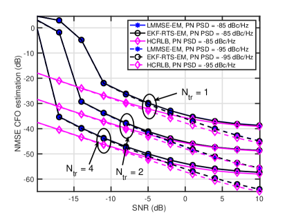
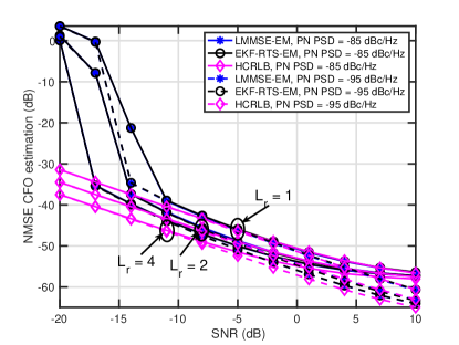
(a)	(b)

Figure 4: Evolution of the NMSE of the CFO estimates obtained using the proposed algorithms versus $\mathop{\mathrm{SNR}}$. The hybrid CRLB is also provided as a performance bound.

Several observations can be made from Fig. 4:

• The proposed LMMSE-EM and EKF-RTS-EM algorithms exhibit very similar estimation performance, which suggests that the proposed EKF-RTS-EM algorithm does not compromise estimation performance while dramatically reducing computational complexity during the measurement update in PN estimation.

• The estimation performance of the proposed algorithms exhibits a small gap with respect to the hybrid CRLB. At low SNR, the gap between the NMSE and the hybrid CRLB is more noticeable, but it shrinks as $\mathop{\mathrm{SNR}}\to\infty$. It is also observed that the NMSE and the hybrid CRLB are monotonically decreasing proportionally to the $\mathop{\mathrm{SNR}}$. There is, however, a certain $\mathop{\mathrm{SNR}}$ value beyond which both the performance of the proposed algorithms and the hybrid CRLB saturate and exhibit a plateau effect. This behavior sets the distinction between the noise-limited regime and the PN-limited regime, whereby estimation performance cannot longer improve even if $\mathop{\mathrm{SNR}}\to\infty$. This behavior is shown in Fig. 5 for $N_{\mathrm{tr}}=4$ and $L_{\mathrm{r}}=4$.

• The estimation performance in the low SNR regime does not depend on the PSD of the PN, which indicates that the synchronization performance is limited by the additive white Gaussian noise (AWGN). Notice, however, that as $\mathop{\mathrm{SNR}}\to\infty$,

• The estimation performance in the low SNR regime does not depend on the PSD of the PN, which indicates that the synchronization performance is limited by the AWGN. Notice, however, that as $\mathop{\mathrm{SNR}}\to\infty$, both the estimation performance of the proposed algorithms and the hybrid CRLB are different for the two values of the PSD $G_{\theta}$ of the PN. Intuitively, as $G_{\theta}$ increases, the information coupling between the PN and the CFO impairments increases, thereby reducing both the achievable CFO estimation performance of the proposed algorithms and the hybrid CRLB. Conversely, reducing $G_{\theta}$ reduces this information coupling, which results in better CFO estimates and lower hybrid CRLB.

• When the $\mathop{\mathrm{SNR}}$ is very low, the NMSE of the proposed algorithms is high. However, when the SNR increases, a waterfall effect is observed, and the $\mathop{\mathrm{SNR}}$ at which this effect happens depends on both the number of RF chains $L_{\mathrm{r}}$ and the number of OFDM training symbols $N_{\mathrm{tr}}$. More especifically, increasing $N_{\mathrm{tr}}$ or $L_{\mathrm{r}}$ shifts the minimum $\mathop{\mathrm{SNR}}$ at which this waterfall effect is observed. Thereby, increasing $N_{\mathrm{tr}}$ and $L_{\mathrm{r}}$ results in more accurate estimates of the CFO parameter, even for $\mathop{\mathrm{SNR}}<-10$ dB.

• Last, increasing the number of OFDM training symbols $N_{\mathrm{tr}}$ and the number of receive RF chains $L_{\mathrm{r}}$ have a different impact on both the CFO estimation performance and the hybrid CRLB. More especifically, doubling $N_{\mathrm{tr}}$ results in a performance gain of approximately $9$ dB, which indicates that the estimation performance depends on $N_{\mathrm{tr}}^{3}$, which is a similar result to the CFO estimation performance and CRLB in [19]. Regarding the number of receive RF chains, doubling $L_{\mathrm{r}}$ enhances estimation performance by a factor of $3$ dB, which indicates that the estimation approach averages the receive noise across multiple receive RF chains, thereby exhibiting an NMSE estimation performance proportional to $L_{\mathrm{r}}^{-1}$.

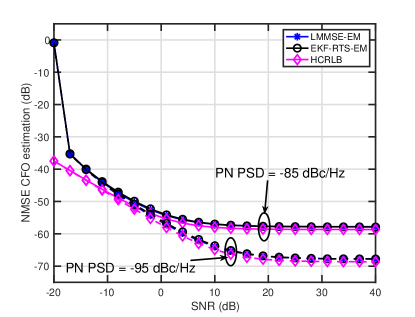
Figure 5: Asymptotic evolution of the NMSE of the CFO estimates obtained using the proposed algorithms versus $\mathop{\mathrm{SNR}}$. The hybrid CRLB is also provided as a performance bound.

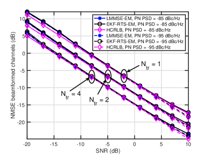
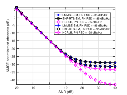
(a)	(b)

Figure 6: Evolution of the NMSE of the beamformed channel estimates obtained using the proposed algorithms versus $\mathop{\mathrm{SNR}}$. The hybrid CRLB is also provided as a performance bound.

In Fig. 6 (a), I show the NMSE evolution of the equivalent beamformed channels versus $\mathop{\mathrm{SNR}}$, for both the proposed LMMSE-EM and the EKF-RTS-EM algorithms. The number of receive RF chains is set to $L_{\mathrm{r}}=4$, and the number of OFDM training symbols $N_{\mathrm{tr}}$ is swept within $\{1,2,4\}$. A similar behavior to that in Fig. 4 is observed. For both proposed algorithms, the estimation performance is very close to the hybrid CRLB, although there is a more noticeable performance gap for $\mathop{\mathrm{SNR}}<10$ dB. Similar to Fig. 4, it is observed that the reduction in computational complexity of the second proposed EKF-RTS-EM algorithm does not compromise estimation performance, thereby showing that synchronization in the low SNR regime can be successfully accomplished with reduced computational complexity. It is also observed that doubling the number of OFDM training symbols $N_{\mathrm{tr}}$ results in enhanced estimation performance by a factor of $3$ dB, which is expected since it was observed that the Fisher information of the channel coefficients increases linearly with the number of training samples.

Furthermore, the performance of the proposed algorithms, as well as the hybrid CRLB, do not depend on the PSD of the PN in both the mid and low SNR regimes. Notice, however, that for $\mathop{\mathrm{SNR}}>0$ dB, the estimation performance and hybrid CRLB depend on the PSD of the PN, similar to Fig. 4. This behavior sets the beginning of the PN-limited regime, which is more pronounced as $\mathop{\mathrm{SNR}}\to\infty$, as shown in Fig. 6 (b). In Fig. 6, the number of OFDM training symbols is set to $N_{\mathrm{tr}}=4$. It is observed that the estimation performance gap between the proposed algorithms and the hybrid CRLB increases as $\mathop{\mathrm{SNR}}\to\infty$, and it is more pronounced for smaller values of the PSD of the PN. This behavior is due to two different factors: i) instead of using the MMSE estimator for the PN, the proposed algorithms attempt to approximate this estimator using statistical linearization (LMMSE), such that non-linearities are not dealt with, and ii) for smaller values of the PSD of the PN, the covariance matrix of the PN has smaller eigenvalues, thereby reducing the amount of prior information on this parameter. This second fact makes the covariance after propagation update be significantly larger than the AWGN impairment, thereby making the Kalman gain for the PN estimator rely more heavily on the measurement and less on the AWGN. Consequently, the PN impairment is more difficult to estimate, which affects the estimation of the equivalent beamformed channels.

Last, I show the estimation performance of the proposed LMMSE-EM and EKF-RTS-EM algorithms versus $\mathop{\mathrm{SNR}}$ in Fig. 7 and Fi.g 8. In Fig. 7, the number of receive RF chains is swept within $\{1,2,4\}$, and it is set to $L_{\mathrm{r}}=4$ in Fig. 8. The PSD of the PN is set to $G_{\theta}=-85$ dB in Fig. 7, which corresponds to a stronger PN process. The number of OFDM training symbols is set to $N_{\mathrm{tr}}=4$ in both Fig. 7 and Fig. 8.

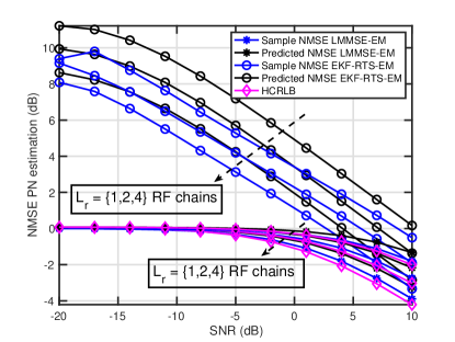
Figure 7: Evolution of the NMSE of the PN estimates obtained using the proposed algorithms versus $\mathop{\mathrm{SNR}}$. The hybrid CRLB is also provided as a performance bound.

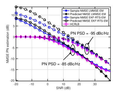
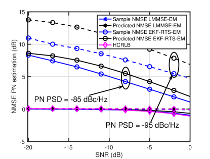
(a)	(b)
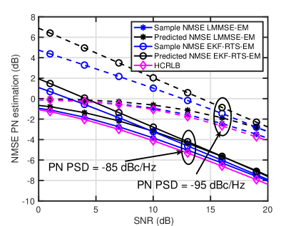
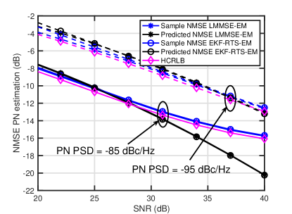
(c)	(d)

Figure 8: Asymptotic evolution of the NMSE of the PN estimates obtained using the proposed algorithms versus $\mathop{\mathrm{SNR}}$. The curves in (a) show this asymptotic evolution for $\mathop{\mathrm{SNR}}$ values between $-20$ and $40$ dB. Magnified curves of the asymptotic evolution are also shown for $\mathop{\mathrm{SNR}}\in[-20,0]$ dB in (b), $\mathop{\mathrm{SNR}}\in[0,20]$ dB in (c), and $\mathop{\mathrm{SNR}}\in[20,40]$ dB in (d). The hybrid CRLB is also provided as a performance bound.

The first observation from both Fig. 7 and Fig. 8 is that the PN estimation performance of the first proposed LMMSE-EM algorithm significantly outperforms that of the second proposed EKF-RTS-EM algorithm. This is not surprising, since the estimation approach in both cases comes from a linearization of the measurement signal through its Jacobian matrix, which is very sensitive to AWGN if a small number of measurements are processed. If a single $L_{\mathrm{r}}$-dimensional measurement is processed, as in the EKF-RTS-EM algorithm, the Jacobian matrix of the measurement varies significantly depending on the AWGN variance and the PSD of the PN process, thereby making it harder for the second proposed algorithm to track the PN variations. If every measurement is processed in a larger-dimensional batch, as in the first proposed LMMSE-EM algorithm, the Kalman measurement update is performed taking the multiple measurements into account, thereby contributing to stabilizing the Jacobian matrix and making it easier to track the PN variations. This is a significant effect only in the low SNR regime, and the performances of both proposed algorithms exhibit convergence as $\mathop{\mathrm{SNR}}$ increases, as shown in Fig. 8.

It is also observed that increasing $L_{\mathrm{r}}$ results in a noise averaging effect, which results in an estimation performance improvement of approximately $3$ dB. This is a similar effect to that in Fig. 6 as a function of $N_{\mathrm{tr}}$, which indicates that the AWGN can be more effectively filtered out as $L_{\mathrm{r}}$ increases.

It is also observed that, for a wide range of $\mathop{\mathrm{SNR}}$ values, the first proposed LMMSE-EM algorithm exhibits estimation performance lying very close to the hybrid CRLB, and divergence from the bound is observed as $\mathop{\mathrm{SNR}}\to\infty$, for similar reasons as with Fig. 6 (b). It is also observed that the NMSE predicted from the first proposed LMMSE-EM algorithm is very close to the actual NMSE performance, while for the second proposed EKF-RTS-EM algorithm it is more difficult to predict the NMSE performance in the low SNR regime, which is expected due to the varying nature of the Jacobian matrix of the measurement when the received samples are sequentially processed, instead of performing simultaneous batch-processing, as in the first proposed LMMSE-EM algorithm.

Finally, in Fig. 9 I show the spectral efficiency evolution as a function of $M$, for $\mathop{\mathrm{SNR}}=\{-10,0\}$ dB, and for PN PSD $G_{\theta}=-85$ dBc/Hz. It is observed that the proposed algorithms cannot accurately estimate the dominant components of the column and row spaces of the broadband channels for $M<32$, and there is slight performance improvement for $M>32$. By comparing $M=32$ with $M=64$, it is observed that the proposed algorithms are able to unlock higher spectral efficiency as the training length increases, but the marginal increase in spectral efficiency does not compensate for doubling the training overhead and computational complexity. This behavior is more pronounced at $\mathop{\mathrm{SNR}}=-10$ dB in Fig. 9 (a), but the same trend can be observed in Fig. 9 (b), for $\mathop{\mathrm{SNR}}=0$ dB.

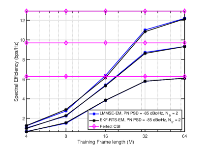
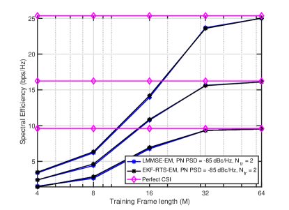
(a)	(b)

Figure 9: Evolution of the spectral efficiency versus number of training frames $M$, obtained using the proposed algorithms for $\mathop{\mathrm{SNR}}=-10$ dB (a) and $\mathop{\mathrm{SNR}}=0$ dB (b). The number of OFDM training symbols is set to $N_{\mathrm{tr}}=2$.

VII Conclusions

In this paper, I proposed a joint synchronization and compressive channel estimation strategy suitable for mmWave MIMO systems using hybrid architectures. Leveraging the available information on the received data, I analyzed and provided closed-form expressions for the hybrid CRLB associated to the synchronization problem, and designed two low-complexity EM-based algorithms to iteratively estimate the TO, CFO, PN and channel impairments. Furthermore, fully leveraging information on the estimates of the unknown parameters, I showed how the obtained channel estimates can be exploited to estimate the high-dimensional frequency-selective mmWave MIMO channel. The numerical results show that the proposed algorithms can be used to estimate the communication channel under the 5G NR wireless channel model, and that near-optimum data rates can be achieved while keeping overhead low and regardless of lack of synchronization.

References

• [1] H. Yan and D. Cabria, “Compressive sensing based initial beamforming training for massive MIMO millimeter-wave systems,” in 2016 IEEE Global Conference on Signal and Information Processing (GlobalSIP), Dec 2016, pp. 620–624.
• [2] H. Yan and D. Cabric, “Compressive initial access and beamforming training for millimeter-wave cellular systems,” IEEE Journal of Selected Topics in Signal Processing, vol. 13, no. 5, pp. 1151–1166, Sep. 2019.
• [3] K. Venugopal, A. Alkhateeb, N. González Prelcic, and R. W. Heath, “Channel estimation for hybrid architecture-based wideband millimeter wave systems,” IEEE Journal on Selected Areas in Communications, vol. 35, no. 9, pp. 1996–2009, Sep. 2017.
• [4] Z. Xiao, P. Xia, and X. G. Xia, “Channel estimation and hybrid precoding for millimeter-wave MIMO systems: A low-complexity overall solution,” IEEE Access, vol. PP, no. 99, pp. 1–1, 2017.
• [5] Z. Marzi, D. Ramasamy, and U. Madhow, “Compressive channel estimation and tracking for large arrays in mm-wave picocells,” IEEE Journal of Selected Topics in Signal Processing, vol. 10, no. 3, pp. 514–527, April 2016.
• [6] Z. Gao, L. Dai, and Z. Wang, “Channel estimation for mmwave massive MIMO based access and backhaul in ultra-dense network,” in Proc. IEEE Int. Conf. on Commun. (ICC), May 2016, pp. 1–6.
• [7] Z. Gao, C. Hu, L. Dai, and Z. Wang, “Channel estimation for millimeter-wave massive MIMO with hybrid precoding over frequency-selective fading channels,” IEEE Communications Letters, vol. 20, no. 6, pp. 1259–1262, June 2016.
• [8] C. Zhang, Z. Xiao, L. Su, L. Zeng, and D. Jin, “Iterative channel estimation and phase noise compensation for SC-FDE based mmwave systems,” in Proc. of 2015 IEEE Int. Conf. on Communication Workshop (ICCW), June 2015, pp. 2133–2138.
• [9] M. Pajovic, P. Wang, T. Koike-Akino, and P. Orlik, “Estimation of frequency unsynchronized millimeter-wave channels,” in 2017 IEEE Global Conference on Signal and Information Processing (GlobalSIP), Nov 2017, pp. 1205–1209.
• [10] N. J. Myers, A. Mezghani, and R. W. Heath, “Swift-link: A compressive beam alignment algorithm for practical mmwave radios,” IEEE Transactions on Signal Processing, vol. 67, no. 4, pp. 1104–1119, Feb 2019.
• [11] N. J. Myers and R. W. Heath, “Message passing-based joint CFO and channel estimation in mmwave systems with one-bit ADCs,” IEEE Transactions on Wireless Communications, vol. 18, no. 6, pp. 3064–3077, June 2019.
• [12] E. Perahia et al, “IEEE 802.11ad: Defining the next generation multi-Gbps Wi-Fi,” in Proc. of IEEE Consumer Commun. and Networking Conf., pp. 1–5, Jan. 2010.
• [13] J. Ko, Y. Cho, S. Hur, T. Kim, J. Park, A. F. Molisch, K. Haneda, M. Peter, D. Park, and D. Cho, “Millimeter-wave channel measurements and analysis for statistical spatial channel model in in-building and urban environments at 28 GHz,” IEEE Transactions on Wireless Communications, vol. 16, no. 9, pp. 5853–5868, Sep. 2017.
• [14] J. T. Parker and P. Schniter, “Parametric bilinear generalized approximate message passing,” IEEE Journal of Selected Topics in Signal Processing, vol. 10, no. 4, pp. 795–808, June 2016.
• [15] N. J. Myers and R. W. Heath, “Joint CFO and channel estimation in millimeter wave systems with one-bit ADCs,” in 2017 IEEE 7th International Workshop on Computational Advances in Multi-Sensor Adaptive Processing (CAMSAP), Dec 2017, pp. 1–5.
• [16] S. Ling and T. Strohmer, “Self-calibration and biconvex compressive sensing,” Inverse Problems, vol. 31, no. 11, p. 115002, 2015.
• [17] J. P. Vila and P. Schniter, “Expectation-maximization Gaussian-mixture approximate message passing,” IEEE Transactions on Signal Processing, vol. 61, no. 19, pp. 4658–4672, Oct 2013.
• [18] A. Alkhateeb, O. El Ayach, G. Leus, and R. W. Heath, “Channel estimation and hybrid precoding for millimeter wave cellular systems,” IEEE Journal of Selected Topics in Signal Processing, vol. 8, no. 5, pp. 831–846, Oct 2014.
• [19] J. Rodríguez-Fernández and N. González-Prelcic, “Channel estimation for hybrid mmwave MIMO systems with CFO uncertainties,” IEEE Transactions on Wireless Communications, vol. 18, no. 10, pp. 4636–4652, Oct 2019.
• [20] 3GPP, “Physical channels and modulation (release 15),” Tech. Rep. v15.1.0, 2017.
• [21] J. Rodríguez-Fernández, N. González-Prelcic, K. Venugopal, and R. W. Heath, “Frequency-domain compressive channel estimation for frequency-selective hybrid millimeter wave MIMO systems,” IEEE Transactions on Wireless Communications, vol. 17, no. 5, pp. 2946–2960, May 2018.
• [22] R. M. Rial, C. Rusu, A. Alkhateeb, N. G. Prelcic, and R. W. Heath Jr., “Hybrid MIMO architectures for millimeter wave communications: Phase shifters or switches?” IEEE Access, no. 99, Jan 2016.
• [23] J. Rodríguez-Fernández, N. González-Prelcic, and R. W. Heath, “A compressive sensing-maximum likelihood approach for off-grid wideband channel estimation at mmwave,” in 2017 IEEE 7th International Workshop on Computational Advances in Multi-Sensor Adaptive Processing (CAMSAP), Dec 2017, pp. 1–5.
• [24] “IEEE draft standard for local and metropolitan area networks - specific requirements - part 11: Wireless lan medium access control (mac) and physical layer (phy) specifications - amendment 3: Enhancements for very high throughput in the 60 ghz band,” IEEE P802.11ad/D8.0, May 2012 (Draft Amendment based on IEEE 802.11-2012), pp. 1–667, June 2012.
• [25] T. A. Thomas, M. Cudak, and T. Kovarik, “Blind phase noise mitigation for a 72 GHz millimeter wave system,” in 2015 IEEE International Conference on Communications (ICC), June 2015, pp. 1352–1357.
• [26] J. Rodriguez-Fernandez and N. Gonzalez-Prelcic, “Joint synchronization, phase noise and compressive channel estimation in hybrid frequency-selective mmwave MIMO systems,” available at arXiv, 2019.
• [27] P. Schniter and A. Sayeed, “Channel estimation and precoder design for millimeter-wave communications: The sparse way,” in Proc. Asilomar Conf. Signals, Syst., Comput., Nov 2014, pp. 273–277.
• [28] R. W. Heath, N. González-Prelcic, S. Rangan, W. Roh, and A. M. Sayeed, “An Overview of Signal Processing Techniques for Millimeter Wave MIMO Systems,” IEEE J. Sel.Topics Signal Process., vol. 10, no. 3, pp. 436–453, April 2016.
• [29] Y. Ghasempour, C. R. C. M. da Silva, C. Cordeiro, and E. W. Knightly, “IEEE 802.11ay: Next-generation 60 GHz communication for 100 Gb/s Wi-Fi,” IEEE Communications Magazine, vol. 55, no. 12, pp. 186–192, Dec 2017.
• [30] J. Rodríguez-Fernández and N. González-Prelcic, “Joint synchronization and compressive estimation for frequency-selective mmwave MIMO systems,” in in Proc. of IEEE Asilomar Conference on Signals, Systems, and Computers, 2018.
• [31] H. L. V. Trees and K. L. Bell, Bayesian Bounds for Parameter Estimation and Nonlinear Filtering/Tracking.   Wiley-IEEE Press, 2007.
• [32] S. M. Kay, Fundamentals of Statistical Signal Processing, Volume I: Estimation Theory.   Prentice Hall PTR, 1993.
• [33] D. D. Lin, R. A. Pacheco, T. J. Lim, and D. Hatzinakos, “Joint estimation of channel response, frequency offset, and phase noise in OFDM,” IEEE Transactions on Signal Processing, vol. 54, no. 9, pp. 3542–3554, Sep. 2006.
• [34] O. H. Salim, A. A. Nasir, H. Mehrpouyan, W. Xiang, S. Durrani, and R. A. Kennedy, “Channel, phase noise, and frequency offset in OFDM systems: Joint estimation, data detection, and hybrid Cramér-Rao lower bound,” IEEE Transactions on Communications, vol. 62, no. 9, pp. 3311–3325, Sep. 2014.
• [35] O. E. Ayach, S. Rajagopal, S. Abu-Surra, Z. Pi, and R. W. Heath, “Spatially sparse precoding in millimeter wave MIMO systems,” IEEE Transactions on Wireless Communications, vol. 13, no. 3, pp. 1499–1513, March 2014.
• [36] S. Särkkä, Bayesian Filtering and Smoothing.   Cambridge University Press, 2013.
• [37] R. W. Heath, Introduction to Wireless Digital Communication: A Signal Processing Perspective.   Prentice Hall, 2017.
• [38] S. Sun, G. R. MacCartney, and T. S. Rappaport, “A novel millimeter-wave channel simulator and applications for 5g wireless communications,” in 2017 IEEE International Conference on Communications (ICC), May 2017, pp. 1–7.
• [39] S. Jaeckel, L. Raschkowski, K. Börner, and L. Thiele, “QuaDRiGa: A 3-D Multi-Cell Channel Model With Time Evolution for Enabling Virtual Field Trials,” IEEE Trans. on Antennas and Propagation, vol. 62, no. 6, pp. 3242–3256, June 2014.
• [40] S. Jaeckel, L. Raschkowski, K. Börner, L. Thiele, F. Burkhardt, and E. Eberlein, “QuaDRiGa: QuaDRiGa - Quasi Deterministic Ratio Channel Generator, User Manual and Documentation,” Fraunhofer Heinrich Hertz Institute, Tech. Rep. v2.0.0, 2017.
• [41] 3GPP, “Study on channel model for frequencies from 0.5 to 100 GHz (release 14.3.0),” Technical Report, Dec 2017.