Disease spreading with social distancing: A prevention strategy in disordered multiplex networks

Abstract

The frequent emergence of diseases with the potential to become threats at local and global scales, such as influenza A(H1N1), SARS, MERS, and recently COVID-19 disease, makes it crucial to keep designing models of disease propagation and strategies to prevent or mitigate their effects in populations. Since isolated systems are exceptionally rare to find in any context, especially in human contact networks, here we examine the susceptible-infected-recovered model of disease spreading in a multiplex network formed by two distinct networks or layers, interconnected through a fraction $q$ of shared individuals (overlap). We model the interactions through weighted networks, because person-to-person interactions are diverse (or disordered); weights represent the contact times of the interactions. Using branching theory supported by simulations, we analyze a social distancing strategy that reduces the average contact time in both layers, where the intensity of the distancing is related to the topology of the layers. We find that the critical values of the distancing intensities, above which an epidemic can be prevented, increase with the overlap $q$. Also we study the effect of the social distancing on the mutual giant component of susceptible individuals, which is crucial to keep the functionality of the system. In addition, we find that for relatively small values of the overlap $q$, social distancing policies might not be needed at all to maintain the functionality of the system.

I Introduction

Localized outbreaks of resurgent or new diseases often have the potential to become epidemics, affecting a relevant proportion of a given region, if no preventive measures are undertaken or mitigation strategies are implemented. Worse still, the high interconnection between cities and also between countries extremely favors the spreading of a disease throughout the entire world, which may turn an outbreak into a pandemic in a matter of months, weeks, or even days. This is what recently happened with COVID-19 disease, declared a pandemic on March 11, 2020, by the World Health Organization World Health Organization (2020a); Cucinotta and Vanelli (2020). Over the last decades researchers across multiple disciplines have been modeling disease propagation to develop strategies that could prevent or at least curtail epidemics (and pandemics, in the worst cases). Infectious diseases usually propagate through physical contacts among individuals Bailey (1975); Anderson and May (1992), and researchers have found that modeling these contact patterns Gonzalez et al. (2008); Cattuto et al. (2010) is best achieved using complex networks Boccaletti et al. (2006); Barrat et al. (2004); Newman (2010); Pastor-Satorras et al. (2015), in which individuals and their interactions are represented by nodes and links, respectively. Numerous disease propagation models have made use of complex networks, including the susceptible-infected-susceptible (SIS) Bailey (1975); Boccaletti et al. (2006); Pastor-Satorras et al. (2015) and susceptible-infected-recovered (SIR) Kermack and McKendrick (1927); Grassberger (1983); Anderson and May (1992); Newman (2002); Boccaletti et al. (2006); Pastor-Satorras et al. (2015) models. In these epidemic models, individuals can be in different states. For example, infected (I) individuals carry the disease and can transmit it to susceptible (S) neighbors that are not immune to the disease, while recovered (R) individuals do not participate in the propagation process because they have either recovered from a previous infection or because they have died. The SIR model, in which individuals acquire permanent immunity after recovering from an illness, is the simplest and most used to study non-recurrent diseases. In the discrete-time version of this model Bailey (1975), at each time step I individuals spread the disease to their S neighbors with the same probability $\beta\in[0,1]$, and switch to the R state $t_{r}$ time steps after being infected, where $t_{r}$ is the recovery time of the disease. The propagation reaches the final stage when the number of I individuals goes to zero. At this stage, the fraction $R$ of recovered individuals indicates the extent of the infection, since all recovered individuals were once infected. In this model, the spreading is controlled by the effective probability of infection $T=1-(1-\beta)^{t_{r}}$, the transmissibility, with $T\in[0,1]$. When $T$ is below a critical value $T_{c}$, also called the epidemic threshold, the fraction $R$ of recovered individuals, which is the order parameter of a continuous phase transition, is negligible compared to the system size $N$, and therefore the system is in a non-epidemic phase. On the other hand, above $T_{c}$ the fraction $R$ is comparable to $N$ and thus it is said that the disease becomes an epidemic Newman (2002); Miller (2007); Kenah and Robins (2007); Lagorio et al. (2009).

In countries such as Italy or Spain, COVID-19 disease spread uncontrollably, causing tens of thousands of deaths, not only because of the intrinsic virulence of the disease, but also due to the collapse of the health system. On the other hand, in countries where the disease arrived after spreading over Europe and the United States, such as Argentina, authorities immediately implemented a preventive massive lockdown, limiting the contact between people. The goal was to avoid the collapse of the health system, to be able to provide rapid and effective medical response to those affected by the disease. Nonetheless, due to the vulnerable economic and social conditions of a vast portion of the Argentinian society, it was practically impossible to completely cut off the interactions between people, which enabled the disease to keep disseminating through the population. Therefore, not only is it important to understand how a disease spreads under different isolation conditions, but it is also crucial to evaluate how it can be mitigated. Vaccination Cohen et al. (2003); Ferrari et al. (2006); Bansal et al. (2006); Pastor-Satorras et al. (2015); Buono and Braunstein (2015); Alvarez-Zuzek et al. (2015); Merler et al. (2016); Di Muro et al. (2018); Alvarez-Zuzek et al. (2019) is regarded as the most efficient measure to prevent or attenuate an epidemic, providing individuals with immunity against a disease. In addition, this pharmacological intervention avoids the negative consequences that society may face after implementing strict and detrimental policies such as partial or complete lockdown and quarantine (e.g., social and economic disruption). However, in emergency situations such as the ongoing COVID-19 pandemic, a vaccine is not yet available and therefore, it is necessary to take other types of countermeasures.

On the other hand, there is a group of strategies less severe than quarantine and lockdown, but in the same spirit. “Social distancing” strategies Gross et al. (2006); Eastwood et al. (2010); Lagorio et al. (2011); Buono et al. (2012); Valdez et al. (2012); Buono et al. (2013); Perez et al. (2020) are a set of actions intended to reduce contact between individuals (shorten the interaction times, maintain a minimum physical distance, avoid crowded places, etc.), with the aim of decreasing the probability of disease transmission. These kinds of strategies respond to the direct transmission mechanism of the virus that causes the COVID-19 disease, although they also apply to diseases that spread in a similar way. The SARS-CoV-2 virus is expelled in the form of droplets from an infected individual through mouth and nose (when talking, exhaling, or coughing), and can enter a healthy individual (located within a 1-2 m range, approximately, and facing the infected individual) through the mucous membranes (eyes, nose, and mouth) World Health Organization (2020b). Therefore, as individuals are more deeply interconnected, the probability of infection significantly increases. Social distancing, along with partial or complete lockdown, has been undertaken in many countries to face the COVID-19 pandemic. Researchers believe that, until a vaccine is widely available, social distancing will remain one of the primary measures to combat the spread of the disease Badr et al. (2020).

One way of modeling social distancing measures is by reducing contact times between individuals. In real-world networks, contact times usually span a broad distribution Cattuto et al. (2010); Karsai et al. (2011); Stehlé et al. (2011). These kinds of systems are known as disordered networks, which are characterized by the existing diversity in the strength or intensity of the interactions among the different parts of the system. Disordered networks have been receiving much attention recently Barrat et al. (2004); Buono et al. (2012, 2013); Perez et al. (2020). In Ref. Perez et al. (2020) disorder is implemented using a weighted complex network Barrat et al. (2004), in which the weights associated with links represent the normalized contact times $\omega$ of the interaction between two individuals. These contact times follow a power-law distribution, $W(\omega)=1/(a\omega)$ that resembles experimental results Cattuto et al. (2010); Karsai et al. (2011); Stehlé et al. (2011). The parameter $a$ is the disorder intensity, which controls the range of contact times in the distribution along with its average value. Also, the interactions between individuals are categorized as either close (larger average contact time) or distant (shorter average contact time), each representing complementary fractions ($f_{1}$ and $1-f_{1}$, respectively) of the total number of interactions. This is carried out by controlling the corresponding disorder intensity of the contact time distributions. Researchers have found that for a system in an epidemic phase, when the fraction $f_{1}$ of close contacts is sufficiently small, increasing the disorder intensity of the distant interactions to decrease their average contact time may switch the system to a non-epidemic phase.

A significantly relevant magnitude to also consider is the size GCS of the giant component of susceptible individuals, or largest connected cluster, at the final stage. This cluster is formed by all the remaining susceptible (healthy) individuals that are connected with each other, and it is the network that sustains the functionality of a society, e.g., the economy of a region. Using a generating function formalism, Newman Newman (2005) showed that in the SIR model there exists a second threshold $T^{*}$ above which the giant cluster of susceptible individuals vanishes at the final stage. On the other hand, Valdez et al. Valdez et al. (2012) showed that $T^{*}$ is an important parameter to determine the efficiency of a mitigation or control strategy, because any strategy that manages to decrease the transmissibility below $T^{*}$ can protect a large and connected cluster of susceptible individuals, even when the system is in an epidemic state.

The previously mentioned studies were carried out using isolated networks, i.e., networks that do not interact with other different networks. Researchers have noted that isolated network models ignore the “external” connections that real-world systems use to communicate with their environment, which usually affect the behavior of the dynamical processes that take place on complex systems Gao et al. (2014); Kivelä et al. (2014); Boccaletti et al. (2014); Kenett et al. (2015). Thus, the modeling of interconnected networks, i.e., networks of networks (NoN) or multilayer networks, has become extremely relevant as it allows a more accurate representation of real systems. The ubiquity of the NoN has encouraged researchers to use them in the study of several topics such as cascading failure Buldyrev et al. (2010); Brummitt et al. (2012); Di Muro et al. (2016), social dynamics Castellano et al. (2009); Galam (2008), and disease propagation Saumell-Mendiola et al. (2012); Cozzo et al. (2013); De Domenico et al. (2016). In particular, the SIR model was simulated and solved theoretically in an overlapped multiplex network Buono et al. (2014) system consisting of two individual networks or layers, in which a fraction $q$ of shared nodes ($q$ overlap) is present in both layers. These shared individuals connect the different layers, and their presence makes diseases more likely to spread as $q$ increases Buono et al. (2014).

We believe that the aforementioned aspects are rather relevant to consider, especially taking into account the ongoing COVID-19 pandemic. We aim to include them in a model that reflects, to some extent, the situation that many regions are facing nowadays. In this paper we study a disease-spreading process using the SIR model in an overlapped two-layer multiplex network. The layers, $A$ and $B$, have definite degree distributions and are connected through a fraction $q$ of shared nodes. They also have a distribution of normalized contact times, with disorder intensities $a_{A}$ and $a_{B}$, which are related through the topology of both layers. Based on this model, we implement a social distancing strategy in which the average contact times between individuals in both layers are reduced, and the disorder intensities may be different in each layer. This could reflect the fact that people within their homes have more prolonged interactions, while protective measures increase to reduce the contact times when they go to work or they use public transport. We use the branching theory, supported by extensive simulations, to study this social distancing strategy, and evaluate its effectiveness in preventing the onset of an epidemic. In addition, the ultimate goal is to analyze how the social distancing policies can protect the mutual giant component of susceptible individuals, formed by the healthy individuals participating in both layers, which is what keeps the economy of a region running. We apply this strategy in a variety of multiplex networks with different degree distributions, to explore the effect of network structure.

II Model: Social distancing strategy

We use an overlapped multiplex network formed by two layers, $A$ and $B$, in which a fraction $q$ of nodes, called shared nodes, are present in both layers. For the construction of the layers, both of which are of size $N$, we use the Molloy-Reed algorithm Molloy and Reed (1995). Each layer has its own uncorrelated degree distribution $P_{i}(k)$, which gives the probability that a node has $k$ neighbors in layer $i=A,B$. The connectivity $k$ is limited by a minimum and a maximum value, which we denote as $k^{i}_{\rm min}$ and $k^{i}_{\rm max}$ respectively. On the one hand, we use a homogeneous Poisson distribution $P(k)=e^{-\langle k\rangle}\langle k\rangle^{k}/k!$, in which the average connectivity $\langle k\rangle$ is also the most likely value. A network with such degree distribution is known as an ER (Erdős-Rényi) network Erdős and Rényi (1959). In addition, we use a heterogeneous power-law or scale-free (SF) distribution with exponential cutoff $k_{c}$, $P(k)\propto k^{-\lambda}e^{-k/k_{c}}$, which is more representative of real-world networks as usually some individuals may have a high number of contacts, while the majority may have only a few Newman (2002). We consider the exponential cutoff $k_{c}$ in the power-law distribution as real-world networks are finite and the maximum number of connections of a node is limited by the size of the system. Additionally, each layer is a weighted network in which a link $j$ of layer $i$ has associated a weight $\omega_{ij}$, where $\omega_{ij}$ is a normalized contact time that defines the intensity of the interaction between the two individuals connected by that link. The $\omega_{ij}$ values are taken from the theoretical distribution $W_{i}(\omega_{i})=1/(a_{i}\,\omega_{i})$ Buono et al. (2012); Perez et al. (2020), $\omega_{i}\,\epsilon\,[e^{-a_{i}},1]$, where $a_{i}$ is the disorder intensity of layer $i=A,B$. Therefore, each link of the network is assigned a weight $\omega_{ij}=e^{-a_{i}r_{j}}$ Braunstein et al. (2007), where $r_{j}$ is a random number within the interval $[0,1]$.

To simulate the disease spread, we use the SIR model taking into account that the probability of infection depends not only on the type of disease, but also on the intensity of the interactions between individuals. All individuals are initially susceptible (S), except for one that randomly becomes infected, called patient zero. At each time step, infected individuals (I) spread the disease to susceptible neighbors with a probability $\beta\omega_{i}$, where $\beta$ is the intrinsic infectivity of the disease, and infected individuals recover (R) after $t_{r}$ time steps. We remark that bridge nodes, i.e., the individuals present in both layers, change their state (if they become infected or get recovered) simultaneously in both layers. The propagation stops when the number of infected individuals is zero in both layers. By using the model described above, we can write the transmissibility of the disease in layer $i=A,B$ as $T_{a_{i}}=\sum_{t=1}^{t_{r}}[(1-\beta e^{-a_{i}})^{t}-(1-\beta)^{t}]/(a_{i}t)$ Valdez et al. (2013). Note that $T_{a_{i}}$ is a decreasing function of the disorder intensity $a_{i}$ because, since $\omega_{i}\,\epsilon\,[e^{-a_{i}},1]$, for higher $a_{i}$ values shorter contact times become more probable, and hence the disease is less likely to propagate. In the limit $a_{i}\rightarrow\infty$ we have that $T_{a_{i}}\rightarrow 0$, which is a complete lockdown scenario where each individual is isolated from the rest. On the other hand, in the limit $a_{i}\rightarrow 0$ there is no disorder in layer $i$, then the infection probabilities throughout layer $i$ are all simply equal to $\beta$, recovering the original SIR model in which the transmissibility is $T_{a_{i}}\rightarrow T=1-(1-\beta)^{t_{r}}$.

Setting different $a_{i}$ values allows us to implement a particular social distancing intensity in each layer. Inspired by the current events related to the COVID-19 pandemic and the policies undertaken by authorities in many countries, we describe next the implementation of our social distancing strategy. We assume that the population can be divided into two layers. One layer represents people who stay in their homes, where interactions are more intimate and usually have a prolonged duration. The other layer represents social interactions in environments where precaution measures are undertaken more strictly, such as workplaces, public transport, or grocery shops. In this structured system, it is reasonable that a fraction $q$ of individuals may belong to both groups of people, e.g., essential workers (food supply and distribution systems, sanitary system, public transport, etc.). We propose that the social distancing policies undertaken in each layer are related through their topology, setting $a_{B}=a_{A}\kappa_{B}/\kappa_{A}$. The factor $\kappa_{i}=\langle k^{2}_{i}\rangle/\langle k_{i}\rangle$ is the branching factor Grassberger (1983); Newman (2002) of layer $i=A,B$, where $\langle k_{i}\rangle$ and $\langle k^{2}_{i}\rangle$ are the first and second moments of the degree distribution $P_{i}(k)$, respectively. We remark that for an ER layer the branching factor increases with the average connectivity as $\kappa=\langle k\rangle+1$, while in a SF layer with exponential cutoff $\kappa$ increases as the heterogeneity parameter $\lambda$ decreases. In this way, if layer $B$ represents the social contacts outside the households, where it is expected a more heterogeneous distribution of the interactions, we have $\kappa_{B}>\kappa_{A}$ and hence $a_{B}>a_{A}$; this means that a stronger distancing policy is implemented in layer $B$ to counter the structure effects over the spread of the disease in that layer (see Sec.III.1). We remark that, in our model, the social distancing strategy is static and is applied from the start of the propagation of the disease, distributing fixed weights to the links. This could represent an optimistic scenario, where the authorities of a particular region (e.g., city or country) are well informed about the existence of an infectious disease, and they immediately undertake inflexible measures to get the most out of them.

Finally, we define the relevant magnitudes of the model, at the final stage, in which we focus to study our distancing strategy. On the one hand, $R$ is the relative size of the giant component of recovered individuals, which is formed by all the individuals in the multiplex network that get infected. On the other hand, GCS is the relative size of the mutual giant component of susceptible individuals, composed of susceptible individuals that are connected within a layer and between the two layers of the multiplex network. Depending on the context, we will use GCS to refer to the mutual giant component of susceptible individuals or to its relative size. Note that the GCS is not defined in the absence of overlap, i.e., for $q=0$.

Considering the model presented, for the analysis of the proposed strategy we examine disease parameters $\beta$ and $t_{r}$ so that the system enters an epidemic phase without disorder, i.e., $R>0$ for $a_{A}=a_{B}=0$ (thus the interactions in both layers have the largest temporal duration). We want to analyze whether or not we can find a pair of critical disorder intensity values $(a_{Ac},a_{Bc})$ that prevent the disease from becoming an epidemic, and study how they depend on the fraction $q$ of shared nodes. In addition, we look for critical disorder intensity values $(a^{*}_{A},a^{*}_{B})$ that can prevent the GCS from falling apart, which would certainly cause a significant disruption in the economy of a region or country (a scenario characterized by GCS$\,\,=0$). In the next section, we develop a theoretical approach that facilitates the analysis of the phase space for $R$ and GCS.

III Theory: Results at the final stage

III.1 Phase space for $R$

It has been demonstrated that in isolated networks the final stage of the SIR model Kermack and McKendrick (1927); Grassberger (1983); Anderson and May (1992); Newman (2002); Boccaletti et al. (2006); Pastor-Satorras et al. (2015) maps exactly into link percolation Newman et al. (2001); Newman (2002); Braunstein et al. (2007) in which links between nodes are occupied with probability $p$. Thus, the relevant magnitudes of this model can be obtained theoretically. The mapping holds in the thermodynamic limit, where $N\rightarrow\infty$, and considering that the number of recovered individuals is zero unless they are above a threshold $s_{c}$ Lagorio et al. (2009), which distinguishes between an epidemic and a small outbreak. In isolated complex networks, the critical transmissibility for which the system switches from an epidemic to a non-epidemic phase is $T_{c}=1/(\kappa-1)$, where $\kappa$ is the branching factor  Grassberger (1983); Newman (2002) of the network.

Next we proceed to map the final stage of our model into link percolation using the branching theory and the generating functions framework Newman et al. (2001); Newman (2002, 2003); Braunstein et al. (2007); Wang et al. (2017). Given a two-layer multiplex network with overlap $0<q\leq 1$, we can write a system of transcendental coupled equations for $f_{i}(T_{A},T_{B})\equiv f_{i}$, which is the probability that a branch of infection (formed by recovered individuals) that originates from a random link in layer $i=A,B$ expands infinitely through any of the layers,

$$f_{A} =(1-q)(1-G_{1}^{A}(1-T_{A}f_{A}))\,+q(1-G_{1}^{A}(1-T_{A}f_{A})G_{0}^{B}(1-T_{B}f_{B})),$$ (1)

$$f_{B} =(1-q)(1-G_{1}^{B}(1-T_{B}f_{B}))\,+q(1-G_{1}^{B}(1-T_{B}f_{B})G_{0}^{A}(1-T_{A}f_{A})),$$ (2)

where $G_{0}^{i}(x)=\sum_{k}P_{i}(k)x^{k}$ and $G_{1}^{i}(x)=\sum_{k}(kP_{i}(k)/\langle k_{i}\rangle)x^{k-1}={G_{0}^{i}}^{\prime}(x)/{G_{0}^{i}}^{\prime}(1)$ (with $G^{\prime}\equiv dG/dx$ and $G_{0}^{\prime}(1)=\langle k\rangle$) are the generating functions of the degree and the excess degree distributions, respectively Newman et al. (2001); Newman (2002, 2003); Braunstein et al. (2007); Wang et al. (2017). Note that the factor $G_{1}^{i}(x)$, with $x=1-T_{i}f_{i}$, is the probability that in layer $i$ a branch of infection reaches a node with connectivity $k$, so that it cannot keep extending through its $k-1$ remaining connections. In a similar way, $G_{0}^{i}(x)$ is the probability that a randomly chosen node is not reached by a branch of infection through its $k$ connections in layer $i$. Thus, $f_{A}$ is the sum of two main terms. First, the probability of reaching an individual present only in layer $A$ (with probability $1-q$) so that the branch of infection expands through any of the $k-1$ remaining connections of the individual in that layer, and, second, the probability of reaching one of the shared nodes (with probability $q$) so that the branch of infection expands through any of its $k-1$ contacts in layer $A$ or through any of its $k$ connections in layer $B$ (see Fig. 1).

\begin{overpic}[width=212.47617pt]{fig1a-multiplex-network-inicial} \put(0.0,51.0){\bf{(a)}} \end{overpic}

(a)

\begin{overpic}[width=212.47617pt]{fig1b-multiplex-network-final} \put(0.0,51.0){\bf{(b)}} \end{overpic}

(b)

Figure 1: Scheme of a disordered multiplex network formed by two overlapped layers, $A$ and $B$. The size of the layers is $N_{A}=N_{B}=15$, and the fraction of nodes present in both layers is $q=3/15=0.2$ (vertical lines are used as a guide to show the shared nodes, which are represented by boxes). The thickness of the segments represents the diversity of the normalized contact times $\omega_{ij}$ between individuals. (a) Initially, all the individuals are in the susceptible (S) state, except for an infected (I) node, which kick-starts the propagation of the disease. (b) At the final stage, the recovered (R) individuals are connected by the branches of infection, which originate from the link denoted by a red arrow. One of the branches, denoted by dotted lines, corresponds to the spread of the disease only through layer $A$, and is represented by the first term in Eq. (1). The other branch, denoted by dash-dotted lines, is a branch of infection that spreads through both layers and is represented by the second term in Eq. (1).

An analogous interpretation holds for $f_{B}$. Once we calculate the non-trivial roots of Eqs. (1) and  (2), then the fractions $R_{A}$, $R_{B}$, and $R$ of recovered individuals (i.e., those reached by the branches of infection) can be obtained from

$$R_{A} = (1-q)(1-G_{0}^{A}(1-T_{A}f_{A}))\,+\xi_{R},$$ (3)

$$R_{B} = (1-q)(1-G_{0}^{B}(1-T_{B}f_{B}))\,+\xi_{R},$$ (4)

$$R = (R_{A}+R_{B}-\xi_{R})/(2-q),$$ (5)

where $\xi_{R}=q(1-G_{0}^{A}(1-T_{A}f_{A})G_{0}^{B}(1-T_{B}f_{B}))$ is the fraction of shared recovered nodes at the final stage. The factor $2-q$ in Eq. (5) accounts for the total number of individuals in the system, which is $(2-q)N$. In Sec. IV we show the agreement between the presented equations and the simulations of the model. Generally, if there are critical disorder intensities $(a_{Ac},a_{Bc})$ for a given $q$ value, these can be computed by solving the system of equations formed by $a_{Bc}=a_{Ac}\kappa_{B}/\kappa_{A}$ and the equation det$(J^{f}-I)=0$ evaluated at $f_{A}=f_{B}=0$ (since at the critical point none of the branches of infection expands infinitely). Here $I$ is the identity matrix and $J^{f}$ is the Jacobian matrix of the system of Eqs. (1) and (2), $J^{f}_{i,k}=\partial f_{i}/\partial f_{j}$, then

$$J^{f}|_{f_{A}=f_{B}=\,0}=\left({\begin{array}[]{cc}T_{A}(\kappa_{A}-1)&qT_{B}\langle k_{B}\rangle\\ qT_{A}\langle k_{A}\rangle&T_{B}(\kappa_{B}-1)\\ \end{array}}\right),$$

where $\kappa_{i}$ and $\langle k_{i}\rangle$ are the branching factor and the average connectivity in layer $i=A,B$. The critical disorder intensities $(a_{Ac},a_{Bc})$ are given by the system

$$a_{Bc} = a_{Ac}\frac{\kappa_{B}}{\kappa_{A}},$$ (6)

$$T_{Bc} = \frac{T_{Ac}(\kappa_{A}-1)-1}{[T_{Ac}(\kappa_{A}-1)-1](\kappa_{B}-1)-q^{2}T_{Ac}\langle k_{A}\rangle\langle k_{B}\rangle},$$ (7)

which we solve numerically for $q\,\epsilon\,[0,1]$, and where $T_{Ac}\equiv T_{A}(a_{Ac})$, $T_{Bc}\equiv T_{B}(a_{Bc})$, and $a_{Bc}\equiv a_{Bc}(a_{Ac})$. Note that Eq. (7) differs from the one obtained in Ref. Buono et al. (2014), where both layers of the multiplex network have the same transmissibility $T$, which yields a quadratic equation for $T_{c}$ (the critical transmissibility) with only one stable solution. The result expressed by Eq. (7) reflects the case where no relation between the disorder intensities is implemented, meaning that for every $a_{A}$ value could be a critical value $a_{Bc}$, maintaining a fixed overlap $q$.

In Fig. 2 we show phase diagrams for $R$ on the $(q,a_{A})$ and $(q,a_{B})$ planes, where we use two layers with different degree distributions. The selected parameters for the disease are $\beta=0.1$ and $t_{r}=5$.

\begin{overpic}[width=212.47617pt]{fig2a-aA-q} \put(50.5,0.0){\bf{(a)}} \end{overpic}

(a)

\begin{overpic}[width=212.47617pt]{fig2b-aA-q} \put(50.5,0.0){\bf{(b)}} \end{overpic}

(b)

Figure 2: Phase diagrams for $R$ on the $(q,a_{A})$ and $(q,a_{B})$ planes. (a) Diagrams for an ER layer with different values of $\langle k_{A}\rangle$ and a SF layer with $\lambda_{B}=2.5$ and cutoff $k^{B}_{c}=20$. The solid and black curves represent the critical disorder intensity $a_{Ac}$ (left-hand) and $a_{Bc}$ (right-hand) for $\langle k_{A}\rangle=3,4,5,6,7$, from bottom to top. (b) Diagrams for an ER layer wih $\langle k_{A}\rangle=5$ and a SF layer with cutoff $k^{B}_{c}=20$ and $\lambda_{B}=2.1,2.3,2.5,2.7,2.9$, from top to bottom. Colored regions below the critical curves indicate epidemic phases ($R>0$), which expand as the overlap $q$ increases. Note that in (a) the increase of $\langle k_{A}\rangle$ causes a major increment on the critical intensities of layer $A$, while in $B$ the increment is smaller. A similar effect occurs in (b), when decreasing $\lambda_{B}$. The remaining parameters of the layers are $k^{A}_{\rm min}=0$, $k^{A}_{\rm max}=20$, $k^{B}_{\rm min}=2$, and $k^{B}_{\rm max}=250$.

In Fig. 2 (a) we use an ER layer with variable $\langle k_{A}\rangle$ and a SF layer with $\lambda_{B}=2$ and cutoff $k^{B}_{c}=20$. On the left side of the figure, the curves show the critical values $a_{Ac}$ as a function of the overlap $q$ between the layers, for the different values of $\langle k_{A}\rangle$. The colored regions correspond to the epidemic phase, where $R>0$, for a given $\langle k_{A}\rangle$ value, while above the critical curves the system presents an epidemic-free phase, where $R=0$. The corresponding critical values $a_{Bc}$ for the disorder intensity in layer $B$ are plotted alongside, considering Eq. (6). Fig. 2 (b) shows the critical curves for an ER layer with $\langle k_{A}\rangle=4$ and a SF layer with variable $\lambda_{B}$. As expected in all the cases, the increase of the overlap $q$ causes the epidemic regions to expand, since the spread of the disease is favored by the individuals that propagate it through both layers. This means that the distancing needed to halt the epidemic must be stronger in both layers, thus decreasing the average duration of the interactions. We also observe that the increase of $\kappa_{i}$ (due to the increase of $\langle k_{A}\rangle$ in Fig. 2 (a) or the decrease of $\lambda_{B}$ in Fig. 2 (b) causes a major increment of the critical intensities in layer $i$, while in the other layer the effect is smaller. In these cases, if the structure of a layer changes in favor of the dissemination of the disease (i.e., increase in $\kappa_{i}$) while the other remains unchanged, much of the additional distancing necessary to avoid an epidemic falls on the altered layer.

III.2 Phase space for GCS

In what follows we present a set of equations that allow us to calculate the size GCS of the mutual giant component of susceptible individuals of the multiplex network at the final stage of the process. It is straightforward to write GCS_A and GCS_B, the fraction of nodes that belong to the giant components of susceptible individuals in layer $A$ and $B$ (i.e., the susceptible individuals connected within each one of the layers), respectively,

$$GCS_{A} =(1-q)(G_{0}^{A}(1-T_{A}f_{A})-G_{0}^{A}(\nu_{A}))\,+\xi_{S},$$ (8)

$$GCS_{B} =(1-q)(G_{0}^{B}(1-T_{B}f_{B})-G_{0}^{B}(\nu_{B}))\,+\xi_{S}.$$ (9)

The first terms takes into account the probability that a node that is part of only one of the layers (with probability $1-q$) belongs to the giant component of that layer. This can be written as the probability that a node of layer $i$ is susceptible ($G_{0}^{i}(1-T_{i}f_{i})$) minus the probability of the node being susceptible but not belonging to the giant component ($G_{0}^{i}(\nu_{i})$). On the other hand, $\xi_{S}=q(G_{0}^{A}(1-T_{A}f_{A})G_{0}^{B}(1-T_{B}f_{B})-G_{0}^{A}(\nu_{A})G_{0}^{B}(\nu_{B}))$ is the fraction of shared nodes that belong to the GCS (the mutual giant component). A node is susceptible and does not belong to the GCS if none of its links lead to susceptible nodes that do belong to the GCS. But, if one of these links connects to an R node, in order to be susceptible, the node cannot have been infected by this R node. Thus, we define $\nu_{i}$ as the probability that a random link from layer $i$ leads to a susceptible node that does not belong to the GCS, or to an R node. However, note that in the last case the link must be unoccupied, with probability $1-T_{i}$. Note that similarly to Eqs. (1) and (2), we can write a set of coupled transcendental equations for the probabilities $\nu_{A}(T_{A},T_{B})\equiv\nu_{A}$ and $\nu_{B}(T_{A},T_{B})\equiv\nu_{B}$,

$$\nu_{A} =(1-T_{A})f_{A}+(1-q)G_{1}^{A}(\nu_{A})+qG_{1}^{A}(\nu_{A})G_{0}^{B}(\nu_{B}),$$ (10)

$$\nu_{B} =(1-T_{B})f_{B}+(1-q)G_{1}^{B}(\nu_{B})+qG_{1}^{B}(\nu_{B})G_{0}^{A}(\nu_{A}).$$ (11)

From left to right, the first term is the probability that a random link in layer $i$ leads to a recovered node, which is $f_{i}$ but considering that the link is unoccupied, with probability $1-T_{i}$. The second is the probability that the random link connects to a node that belongs only to layer $i$ (with probability $1-q$), so that none of its outgoing links lead to susceptible nodes belonging to the GCS, nor any of its outgoing links leads to a recovered node and is occupied. Finally, the last term is similar to the second, but the random link in layer $i$ leads to a shared node (with probability $q$) so that besides its outgoings links in layer $i$, none of its links in layer $j$ connect to susceptible nodes that are part of the GCS, and none of its links connects to a recovered node and is occupied. Once the values of $\nu_{i}$ and consequently GCS_i for $i=A,B$ are obtained from Eqs. (8-11), the size of the GCS can be computed as

$$GCS=(GCS_{A}+GCS_{B}-\xi_{S})/(2-q).$$ (12)

In Sec. IV we show the agreement between the equations presented and the simulations of the model.

To study the phase space for the GCS, we define $\mu_{i}$ as the probability that a random link in layer $i=A,B$ connects to a node belonging to the GCS (similarly to what was done in Sec. III.1 with $f_{i}$ for the recovered individuals). Recall that $\nu_{i}$ is the probability that a random link connects to an S node which does not belong to the GCS or that it connects to an R node but considering that the link is unoccupied with probability $1-T_{i}$. Then we have that $\mu_{i}=1-(\nu_{i}+T_{i}f_{i})$, and we obtain a system of equations for $\mu_{A}$ and $\mu_{B}$:

$$\mu_{A} =1-f_{A}-(1-q)G_{1}^{A}(u_{A}-\mu_{A})-qG_{1}^{A}(u_{A}-\mu_{A})G_{0}^{B}(u_{B}-\mu_{B}),$$ (13)

$$\mu_{B} =1-f_{B}-(1-q)G_{1}^{B}(u_{B}-\mu_{B})-qG_{1}^{B}(u_{B}-\mu_{B})G_{0}^{A}(u_{A}-\mu_{A}),$$ (14)

where $u_{i}\equiv 1-T_{i}f_{i}$. If there are critical disorder intensities $(a^{*}_{A},a^{*}_{B})$ for a given $q$ value, these can be computed by solving the system of equations formed by $a^{*}_{B}=a^{*}_{A}\kappa_{B}/\kappa_{A}$, the equation det$(J^{\mu}-I)=0$ evaluated at $\mu_{A}=\mu_{B}=0$ and Eqs. (1) and (2) for $f_{A}$ and $f_{B}$, respectively. Here $J^{\mu}$ is the Jacobian matrix of the system of Eqs. (13) and (14), $J^{\mu}_{i,k}=\partial\mu_{i}/\partial\mu_{j}$, then

$$J^{\mu}|_{\mu_{A}=\mu_{B}=\,0}=\left({\begin{array}[]{cc}(1-q){G_{1}^{A}}^{\prime}(u_{A})+q{G_{1}^{A}}^{\prime}(u_{A})G_{0}^{B}(u_{B})&qG_{1}^{A}(u_{A})G_{1}^{B}(u_{B})\langle k_{B}\rangle\\ qG_{1}^{B}(u_{B})G_{1}^{A}(u_{A})\langle k_{A}\rangle&(1-q){G_{1}^{B}}^{\prime}(u_{B})+q{G_{1}^{B}}^{\prime}(u_{B})G_{0}^{A}(u_{A})\\ \end{array}}\right),$$

where $u_{A}\equiv u_{A}(a^{*}_{A},f_{A})$, $u_{B}\equiv u_{B}(a^{*}_{B},f_{B})$, and $a^{*}_{B}\equiv a^{*}_{B}(a^{*}_{A})$. We solve this system numerically for $q\,\epsilon\,(0,1]$, since the GCS (the mutual giant component of susceptible individuals) is not defined in the absence of overlap, i.e., for $q=0$.

In Fig. 3 we show phase diagrams for GCS on the $(q,a_{A})$ and $(q,a_{B})$ planes, where we use two layers with different degree distributions (the same layers that we used for $R$ in Fig. 2). The selected parameters for the disease are $\beta=0.1$ and $t_{r}=5$.

\begin{overpic}[width=212.47617pt]{fig3a-aA-q} \put(51.5,0.0){\bf{(a)}} \end{overpic}

(a)

\begin{overpic}[width=212.47617pt]{fig3b-aA-q} \put(51.5,0.0){\bf{(b)}} \end{overpic}

(b)

Figure 3: Phase diagrams for GCS on the $(q,a_{A})$ and $(q,a_{B})$ planes. (a) Diagrams for an ER layer with different values of $\langle k_{A}\rangle$ and a SF layer with $\lambda_{B}=2.5$ and cutoff $k^{B}_{c}=20$. The solid and black curves represent the critical disorder intensity $a^{*}_{A}$ (left-hand) and $a^{*}_{B}$ (right-hand) for $\langle k_{A}\rangle=3,4,5,6,7$, from bottom to top. (b) Diagrams for an ER layer wih $\langle k_{A}\rangle=5$ and a SF layer with cutoff $k^{B}_{c}=20$ and $\lambda_{B}=2.1,2.3,2.5,2.7,2.9$, from top to bottom. Colored regions below the critical curves indicate non-functional phases (GCS$\,\,=0$), and functional phases (GCS$\,\,>0$) above the curves. Unlike the results shown in the phase diagrams for $R$, in this case the critical intensities may vanish, i.e., $a^{*}_{A}=a^{*}_{B}=0$, if the overlap $q$ is relatively small. This means that the functionality of the GCS is ensured, independently of the intensity of the implemented distancing strategy.

In Fig. 3 (a) we use an ER layer with variable $\langle k_{A}\rangle$ and a SF layer with $\lambda_{B}=2$ and cutoff $k^{B}_{c}=20$. On the left side of the figure, the curves show the critical values $a^{*}_{A}$ as a function of the overlap $q$ between the layers, for the different values of $\langle k_{A}\rangle$. The colored regions correspond to the non-functional phase, where GCS$\,\,=0$, for a given $\langle k_{A}\rangle$ value, while above the critical curves the system presents a functional phase, where GCS$\,\,>0$. The corresponding critical values $a^{*}_{B}$ for the disorder intensity in layer $B$ are plotted alongside, considering Eq. (6). Fig. 3 (b) shows the critical curves for an ER layer with $\langle k_{A}\rangle=4$ and a SF layer with variable $\lambda_{B}$. As we observe, there are similarities between these results and the phase diagrams presented for $R$. On the one hand, the increase of $\kappa_{i}$ causes a major increment in layer $i$ of the distancing necessary to protect the GCS, while in the remaining layer the change is smaller. However, we note that there is a range of $q$ values in which the critical disorder intensities vanish, i.e., $a^{*}_{A}=a^{*}_{B}=0$. This range depends on the parameters of each particular multiplex network and decreases with $\kappa_{i}$, as can be seen in Figs. 3 (a) and (b). In this region, the GCS exists even when a distancing strategy is not implemented in any layer, thus the system does not lose its functionality. For values of the overlap $q$ that exceed this range, the system needs a minimum distancing to avoid the collapse of the GCS, and an increase of $q$ causes the non-functional regions to expand.

Next we present the summarized results of the social distancing strategy proposed. Looking at an individual case of the multiplex networks previously presented, in Fig. 4 we show the critical curves for $R$ and GCS, the sizes of the giant components of susceptible and recovered individuals throughout the entire system, respectively.

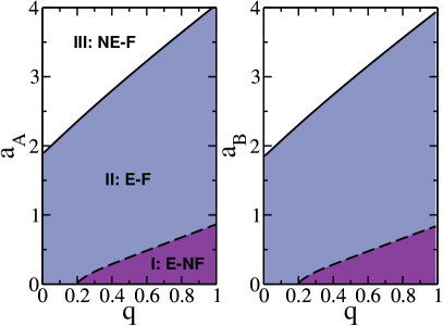
Figure 4: Typical outcomes of the social distancing strategy applied to a multiplex network. Solid and dashed lines represent the critical curves for $R$ and GCS, respectively. In region I of the diagram the social distancing policies are rather weak, leading not only to an epidemic, but also to the crumbling of the GCS, which disrupts the functionality of the system (E-NF phase). As the policies are intensified, in region II, the GCS is prevented from falling apart, while the emergence of an epidemic becomes less likely (E-F phase). In region III, a strict enough social distancing policy (i.e., high disorder intensities in both layers) ensures the system lies on a non-epidemic and functional phase (NE-F phase), which is the best possible scenario. For the presented results, we use an ER layer with $\langle k_{A}\rangle=5$ and a SF layer with $\lambda_{B}=2.5$ and cutoff $k^{B}_{c}=20$. Also, we consider a disease with $\beta=0.1$ and $t_{r}=5$.

We observe now that the phase diagram is divided into three regions. In region I the disease is certainly likely to spread because the disorder intensities implemented in both layers are quite low, which not only fails to prevent an epidemic but also makes the GCS fall apart, causing the system to collapse (E-NF phase). It may happen that even in the absence of a distancing strategy the system does not lose the functionality (i.e., GCS$\,\,>0$ for $a_{A}=a_{B}=0$). This depends on the structure of the multiplex network system (the $\kappa_{B}/\kappa_{A}$ relation) and occurs only for relatively small values of the overlap $q$ (in Fig. 4, for $q<0.2$ approximately). As distancing increases, in region II the epidemic still can not be avoided, but there emerges a GCS, which means that the system remains functional (E-F phase). Finally, region I corresponds to a non-epidemic and functional phase (NE-F), the best possible scenario, in which the disorder intensities in both layers are high enough, i.e., social distancing measures are undertaken intensively. In this region, the system avoids an epidemic and maintains its functionality. Considering this, even though the social distancing efforts may not prevent that a particular disease extends through a significant portion of the population (regions I and II in Fig. 4), they could serve to the purpose of keeping the integrity of the system (regions II and III). It is important to note that, if a GCS remains functional after the end of an epidemic, it is highly recommended not to relax the set of measures undertaken to prevent the transmission of the disease, since there is always the possibility of a second outbreak (originating, for instance, from an imported or undetected case).

Looking forward, we comment on a few elements that we are interested in analyzing in future research. For instance, it is known that nowadays passenger traffic is one of the main causes of the dissemination of a disease across different regions (cities, states, and countries). One way to tackle this issue is to isolate individuals once they arrive to its destination, which is currently being implemented during the COVID-19 pandemic. In this way, it is expected that the passengers cannot spread the disease within the region. To take into account this possibility, instead of using an overlapped multiplex network, we could devise a model in which shared nodes do not belong to both layers, but rather they connect to nodes from other layers according to an inter-layer degree distribution. These nodes would represent individuals that travel to other regions or countries, which are isolated with a certain probability. These considerations may help in deepening the understanding of these processes, encouraging researchers to devise more suitable and efficient strategies for preventing and mitigating the spread of a disease. In addition, it would be relevant to study the temporal evolution of a disease in this scenario, and how it would respond to mitigation measures that are undertaken with some delay.

IV Correspondence between theoretical results and simulations

In this brief section we present a selected set of results from the stochastic simulations of the model established in Sec. II, at the final stage, along with the results computed from the equations obtained in Sec. III. Fig. 5 shows the total fraction $R$ of recovered individuals and the size GCS of the mutual giant component of susceptible individuals that span the entire multiplex network as functions of the disorder intensity $a_{A}$ in layer $A$ (Fig. 5 (a)) and the overlap $q$ (Fig. 5 (b)).

\begin{overpic}[width=195.12767pt]{fig5a-RyGCS-aA} \put(14.0,64.0){\bf{(a)}} \end{overpic}

(a)

\begin{overpic}[width=195.12767pt]{fig5b-RyGCS-q} \put(14.0,63.0){\bf{(b)}} \end{overpic}

(b)

Figure 5: Agreement between theoretical and simulated results. Solid and black lines correspond to theoretical results, while simulations are shown in symbols. (a) Fraction $R$ of recovered individuals (red circles) and the size GCS of the mutual giant component of susceptible individuals (green squares) as functions of the disorder intensity $a_{A}$ in layer $A$, for $q=0.5$. The critical disorder intensities are $a_{Ac}\approx 2.5$, $a_{Bc}\approx 4.5$ for $R$ and $a^{*}_{A}\approx 0.26$, $a^{*}_{B}\approx 0.46$ for GCS. (b) $R$ and GCS as functions of the overlap $q$ between the layers of the multiplex network, for $a_{A}=0.5$. We observe that for $q\approx 0.81$ the GCS collapses, which accounts for the overlap effect over the spread of the disease. For the simulations, we used two layers of size $N=10^{5}$. $P_{A}(k)$ is a Poisson distribution with $\langle k_{A}\rangle=4$, $k^{A}_{\rm min}=0$ and $k^{A}_{\rm max}=40$, while $P_{B}(k)$ is a power-law distribution with cutoff $k_{C}=20$, $\lambda=2$, $k^{B}_{\rm min}=2$ and $k^{B}_{\rm max}=250$.

The solid and black lines correspond to the theoretical results, which agree with the simulations that are represented by symbols. We run $10^{4}$ realizations of the simulations and averaged the results considering only realizations where the number of recovered individuals in each layer was above a threshold $s_{c}=200$ Lagorio et al. (2009).

V Conclusions

We apply the SIR model to study the spread of a disease in an overlapped multiplex network composed of two layers with its own distribution of contact times, in which a fraction $q$ of individuals belong to both layers. We propose a social distancing strategy that reduces the average contact time of the interactions between individuals within each layer. This is achieved by increasing the respective disorder intensities, which are related through the topology of the layers. We find that as the intensity of the distancing increases, the system can go through different phases. For low levels of distancing, the system fails to prevent an epidemic and to protect the functional network. The increment of the measures reduces the spread of the disease, thus taking the system to a functional phase (which is fundamental to keep running the economy of a society) but in an epidemic scenario. Finally, the system reaches an epidemic-free and functional phase for high enough levels of distancing. The critical values increase with the overlap $q$ because the individuals that are shared by the layers ease the spread of the disease, so that more social distancing measures must be undertaken to prevent an epidemic. However, depending on the structure of the multiplex network system, relatively small values of $q$ might allow the system to maintain the functionality, even in the absence of distancing policies. All in all, the control of contact times between individuals can serve as a prevention strategy that overcomes the overlap effect in multiplex networks, preventing not only an epidemic, but also the economic collapse of a region or country, which might be equally harmful for society.