Axiomatizations of betweenness
in order-theoretic trees

Abstract.

The ternary betweenness relation of a tree, $B(x,y,z),$ expresses that the node $y$ is on the unique path between nodes $x$ and $z$. This notion can be extended to order-theoretic trees defined as partial orders such that the set of nodes larger than any node is linearly ordered. In such generalized trees, the unique ”path” between two nodes is linearly ordered and can be infinite.

We generalize some results obtained in a previous article for the betweenness relation of join-trees. Join-trees are order-theoretic trees such that any two nodes have a least upper-bound. The motivation was to define conveniently the rank-width of a countable graph. We called quasi-tree the structure $(N,B)$ based on the betweenness relation $B$ of a join-tree with vertex set $N$. We proved that quasi-trees are axiomatized by a first-order sentence.

Here, we obtain a monadic second-order axiomatization of betweenness in order-theoretic trees. We also define and compare several induced betweenness relations, i.e., restrictions to sets of nodes of the betweenness relations in countable generalized trees of different kinds. We prove that induced betweenness in quasi-trees is characterized by a first-order sentence. The proof uses order-theoretic trees.

Introduction

The rank-width $rwd(G$) of a finite graph $G,$ defined by Oum and Seymour in [17], is a complexity measure based on ternary trees whose leaves hold the vertices. If $H$ is an induced subgraph of $G$, then $rwd(H)\leq rwd(G)$. In order to define the rank-width of a countable graph in such a way that it be the least upper-bound of those of its finite induced subgraphs, we have defined in [6] certain generalized (undirected) trees called quasi-trees (forming the class QT), such that the unique ”path” between any two nodes is linearly ordered and can be infinite. In particular, it can have the order-type of an interval of the set $\mathbb{Q}$ of rational numbers. As no notion of adjacency can be used, we have defined quasi-trees in terms of a notion of betweenness.

The betweenness relation of a tree is the ternary relation $B$ such that $B(x,y,z)$ holds if and only if $x,y,z$ are distinct and $y$ is on the unique path between $x$ and $z$. It can be extended to order-theoretic trees defined as partial orders such that the set of elements larger than any element is linearly ordered. A join-tree is an order-theoretic tree such that any two nodes have a least upper-bound, equivalently in this case, a least common ancestor. A join-tree may have no root, i.e., no largest element. A quasi-tree is defined abstractly as a ternary structure $S=(N,B)$ satisfying finitely many first-order betweenness axioms. But quasi-trees are equivalently characterized as the betweenness relations of join-trees [6].

In the present article we axiomatize in monadic second-order logic betweenness in order-theoretic trees. We also define and study several induced betweenness relations, i.e., restrictions to sets of nodes of betweenness relations in generalized trees of different kinds. An induced betweenness relation in a quasi-tree need not be that of a quasi-tree. However, induced betweenness relations in quasi-trees, forming the class IBQT, are also axiomatized by a single first-order sentence. This fact does not follow immediately by a general logical argument from the first-order characterization of quasi-trees. The proof that this axiomatization is valid uses order-theoretic trees.

We define actually four types of betweenness structures $S=(N,B)$ for which we prove that the inclusions following from the definitions are proper. For each type of betweenness, a structure $S$ is defined from an order-theoretic tree $T$. Except for the case of induced betweenness in order-theoretic trees, some defining tree $T$ can be described in $S$ by monadic second-order formulas. In technical words, $T$ is defined from $S$ by a monadic second-order transduction, a notion thoroughly studied in [11]. The construction of a monadic second-order transduction for induced betweenness in quasi-trees is not straighforward. It is based on a notion of structuring of order-theoretic trees already used in [5, 6, 7], that consists in decompositing them into pairwise disjoint ”branches”, that are convex and linearly ordered. Monadic second-order formulas can identify structurings of order-theoretic trees. In these articles, we also obtained algebraic characterizations of the join-trees and quasi-trees that are the unique countable models of monadic-second order sentences.

In order to provide a concrete view of our generalized trees, we embed them into topological trees, defined as connected unions of possibly unbounded segments of straight lines in the plane that have no subset homeomorphic to a circle. Countable induced betweenness relations in topological trees and in quasi-trees are the same.

Our main results are the following ones:

• this class IBQT is first-order axiomatizable (Theorem 3.1),

• a join-tree witnessing that a ternary structure $S$ is in IBQT can be specified in $S$ by monadic second-order formulas (Theorem 3.25),

• induced betweenness relations in topological trees and in quasi-trees are the same (Theorem 4.4).

About motivations

This article arises from three research directions of theoretical nature. The first one concerns Model Theory. A general goal is to understand the power of logical languages, here first-order (FO in short) and monadic second-order (MSO in short) logic, for expressing properties of trees, graphs and related relational structures, and of transformations of such structures. For finite structures, monadic second-order logic yields tractable algorithms parameterized by appropriate widths, based on hierarchical decompositions [11, 13]. For countably infinite structures described in appropriate finitary ways, it yields decidability results. The relevant graphs and trees belong to Caucal’s hierarchy (see [1, 18, 19]). On both aspects the literature is enormous. When a property is proved to be MSO expressible, we try to answer the natural question of asking whether it is FO expressible.

The second research direction concerns order-theoretic trees (O-trees in short), a classical notion in the Theory of Relations, studied in particular by Fraïssé in [12]. He defined a countable universal O-tree, in which every countable O-tree embeds. We used O-trees for defining rank-width and modular decomposition of countable graphs [6, 10]. Infinite words based on countable linear orders (of any type) are studied with the concepts of the Theory of Automata and monadic second-order logic [2]. Hence, our study of order-theoretic trees with such tools aims at completing this theory of countable structures [5, 7].

The third research direction concerns Combinatorial Geometry and, in particular, the natural notion of betweenness. The betweenness of a linear order describes it up to reversal. This notion is FO axiomatizable, but offers difficult problems and open questions. It is NP-complete to decide if a finite ternary relation is included in the betweenness relation of a linear order (see Chapter 9 of [11]). Betweenness has also been studied in partial orders. It is axiomatized by an infinite set of first-order sentences in [16], that cannot be replaced by a finite one [9]. In the latter article, we axiomatize betweenness in partial orders by an MSO sentence. Several notions of betweenness in graphs have also been investigated and axiomatized. We only refer to the survey [3] that contains a rich bibliography. Another reference is [4] about the betweenness in graphs relative to induced paths: $y$ is between $x$ and $z$ if it is an intermediate vertex on a chordless path between $x$ and $z$.

Summary

We review definitions and notation in Section 1. We define four different notions of betweenness in order-theoretic trees in Section 2. We establish in Section 3 the first-order and monadic second-order axiomatizations presented above. The case of induced betweenness in order-theoretic trees is left as a conjecture. We also examine whether monadic second-order transductions can produce witnessing trees from given betweenness structures. In Section 4, we describe embeddings of join-trees into topological trees. In an appendix (Section 6), we give an example of a first-order class of relational structures (actually of labelled graphs) whose induced substructures do not form a first-order (and even a monadic second-order) axiomatizable class.

1. Definitions and basic facts

All trees, graphs and logical structures are countable, which means, finite or countably infinite. We will not repeat this hypothesis in our statements.

In some cases, we denote by $X\uplus Y$ the union of sets $X$ and $Y$ to insist that they are disjoint. Isomorphism of ordered sets, trees, graphs and other logical structures is denoted by $\simeq$. We denote by $[n]$ the set of integers $\{1,...,n\}$.

The arity of a relation $R$ is $\rho(R).$ The restriction of a relation $R$ defined on a set $V$ to a subset $X$ of $V$, i.e., $R\cap X^{\rho(R)},$ is denoted by $R[X]$. If $S$ is an {$R_{1},..,R_{k}\}$-structure $(V,R_{1},..,R_{k})$, then $S[X]:=(V,R_{1}[X],..,R_{k}[X])$.

The Gaifman graph of $S=(V,R_{1},..,R_{k})$ is the graph $\mathit{Gf}(S)$ with vertex set $V$ and an edge between $x$ and $y\neq x$ if and only if $x$ and $y$ belong to a tuple of some relation $R_{i}$. We say that $S$ is connected if its Gaifman graph is connected. If it is not, $S$ is the disjoint union of connected structures, each of them corresponding to a connected component of the Gaifman graph of $S$.

A family of sets is overlapping if it contains two sets $X$ and $Y$ such that $X\cap Y$, $X-Y$ and $Y-X$ are all not empty.

1.1. Partial orders

For partial orders $\leq,\preceq,\sqsubseteq$, … we denote respectively by $<,\prec,\sqsubset$, … the corresponding strict partial orders. We write $x\bot y$ if $x$ and $y$ are incomparable for the considered order.

Let $(V,\leq)$ be a partial order. For $X,Y\subseteq V$, the notation $X<Y$ means that $x<y$ for every $x\in X$ and $y\in Y$. We write $X<y$ instead of $X<\{y\}$ and similarly for $x<Y$. We use similar notation for $\leq$ and $\bot$. The least upper-bound of $x$ and $y$ is denoted by $x\sqcup y$ if it exists and is called their join.

If $X\subseteq V$, then we define $N_{\leq}(X):=\{y\in V\mid y\leq X\}$ and similarly for $N_{<}$. We define $\downarrow(X):=\{y\in V\mid y\leq x$ for some $x\in X\}.\$We have $N_{\leq}(X)\leq X$, $N_{\leq}(\emptyset)=V$, and $\downarrow(\emptyset)=\emptyset.$ We also define $L_{\geq}(X):=\{y\in V\mid y\geq X\}$, and similarly $L_{>}(X).$ We write $L_{\geq}(x)$ (resp. $L_{\geq}(x,y))$ if $X=\{x\}$ (resp. $X=\{x,y\}$) and similarly for $L_{>}.$ Note that $L_{\geq}(X)$ is $N_{\geq^{\prime}}(X)$ for the opposite order $\leq^{\prime}$ of $\leq.$

An interval $X$ of $(V,\leq)$ is a convex subset, i.e., $y\in X$ if $x<y<z$ and $x,z\in X$.

Let $(V,\leq)$ and $(V^{\prime},\leq^{\prime})$ be partial orders. An embedding $j:(V,\leq)\rightarrow(V^{\prime},$ $\leq^{\prime})$ is an injective mapping such that $x\leq y$ if and only if $j(x)\leq^{\prime}j(y)$; in this case, $(V,\leq)$ is isomorphic by $j$ to $(j(V),\leq^{\prime\prime})$, where $\leq^{\prime\prime}$ is the restriction of $\leq^{\prime}$ to $j(V)$ (i.e., is $\leq^{\prime}\ [j(V)]$). We will write more simply $(j(V),\leq^{\prime})$.

We say that $j$ is a join-embedding if, furthermore, $j(x)\sqcup^{\prime}j(y)$ is defined and equal to $j(x\sqcup y)$ whenever $x\sqcup y$ is defined.

Here is an example of an embedding that is not a join-embedding: $j$ is the inclusion mapping $(X,\leq)\rightarrow(V,\leq)$ where $V:=\{a,b,c,d\}$, $a<c<d$, $b<c$ , $a\bot b$ and $X=\{a,b,d\}$. We have $a\sqcup b=d$ in $(X,\leq)$ but $a\sqcup b=c\neq j(d)$ in $(V,\leq).$

1.2. Trees

A forest is a possibly empty, undirected graph $F$ that has no cycles. Hence, it has neither loops nor multiple edges. We call nodes its vertices. Their set is denoted by $N_{F}$. A tree is a connected forest.

A rooted tree $R=(T,r)$ is a tree $T$ equipped with a distinguished node $r$ called its root. We define on $N_{R}:=N_{T}$ the partial order $\leq_{R}$ such that $x\leq_{R}y$ if and only if $y$ is on the unique path in $T$ between $x$ and the root $r$. The minimal nodes are the leaves and the root is the largest node. The least upper-bound of $x$ and $y$, denoted by $x\sqcup_{R}y$ is their least common ancestor in $R$.

We will specify a rooted tree $R$ by $(N_{R},\leq_{R})$ and we will omit the index $R$ when the considered tree is clear.

A partial order $(N,\leq)$ is $(N_{R},\leq_{R})$ for some rooted tree $R$ if and only if it has a largest element and, for each $x\in N$, the set $L_{\geq}(x)$ is finite and linearly ordered. These conditions imply that any two nodes have a join.

1.3. Order-theoretic forests and trees

Definition 1.1 (O-forests and O-trees). In order to have a simple terminology, we will use the prefix O- to mean order-theoretic.

1. An O-forest is a pair $F=(N,\leq)$ such that:

   1. $N$ is a possibly empty set called the set of nodes,

   2. $\leq$ is a partial order on $N$ such that, for every node $x,$ the set $L_{\geq}(x)$ is linearly ordered.

   It is called an O-tree if furthermore:

   1. every two nodes $x$ and $y$ have an upper-bound.

   An O-forest $F$ is the union of disjoint O-trees $T_{1},T_{2},...$ such that the Gaifman graphs $\mathit{Gf}(T_{i})$ are the connected components of $\mathit{Gf}(F)$. Two nodes of $F$ are in a same O-tree $T_{i}$ if and only if they have an upper-bound.

   The leaves are the minimal elements. If $N$ has a largest element $r$ (i.e., $x\leq r$ for all $x\in N$) then $F$ is a rooted O-tree and $r$ is its root.

2. A line in an O-forest $(N,\leq)$ is a linearly ordered subset $L$ of $N$ that is convex, i.e., such that $y\in L$ if $x,z\in L$ and $x<y<z$. A subset $X$ of $N$ is upwards closed (resp. downwards closed) if $y\in X$ whenever $y>x$ (resp. $y<x$) for some $x\in X$. In an O-forest, the set $L_{\geq}(X)$ of upper-bounds of a nonempty set $X\subseteq N$ is an upwards closed line.

3. An O-tree $T=(N,\leq)$ is a join-tree if every two nodes $x$ and $y$ have a least upper-bound (for $\leq$) denoted by $x\sqcup y$ and called their join (cf. Section 1.1). In a join-tree, every finite set has a least upper-bound, but an infinite one may have none.

4. Let $J=(N,\leq)$ be an O-forest and $X\subseteq N$. Then $J[X]:=(X,\leq)$ is an O-forest. It is the sub-O-forest of $J$ induced on $X$. Two elements $x,y$ having a join $z$ in $J$ may have no join in $J[X]$ or they may have a join different from $z$. If $J$ is an O-tree, then $J[X]$ may not be an O-tree.

Examples 1.2.

1. If $R$ is a rooted tree, then $(N_{R},\leq_{R})$ is a join-tree. Every finite O-tree is a join-tree of this form.

2. Every linear order is a join-tree.

3. Let $S:=\mathbb{N}\cup\{a,b,c\}$ be strictly partially ordered by $<_{S}$ such that $a<_{S}b,c<_{S}b$ and $b<_{S}i<_{S}j$ for all $i,j\in\mathbb{N}$ such that $j<i$, and $a$ and $c$ are incomparable. Then $T:=(S,\leq_{S})$ is a join-tree, see the left part of Figure 1. In particular $a\sqcup_{S}c=b$. The relation $\leq_{S}$ is not the partial order associated with any rooted tree (by the remark at the end of Section 1.2).

   We can consider $\mathbb{N}\cup\{a,b\}$ as forming a ”path” between $a$ and 0 in the join-tree $T$ (where 0 is the largest element). A formal definition of such ”paths” will be given. Let $S^{\prime}:=S-\{b\}.$ The O-tree $T[S^{\prime}]:=(S^{\prime},\leq_{S})$ is not a join-tree because $a$ and $c$ have no join.

   

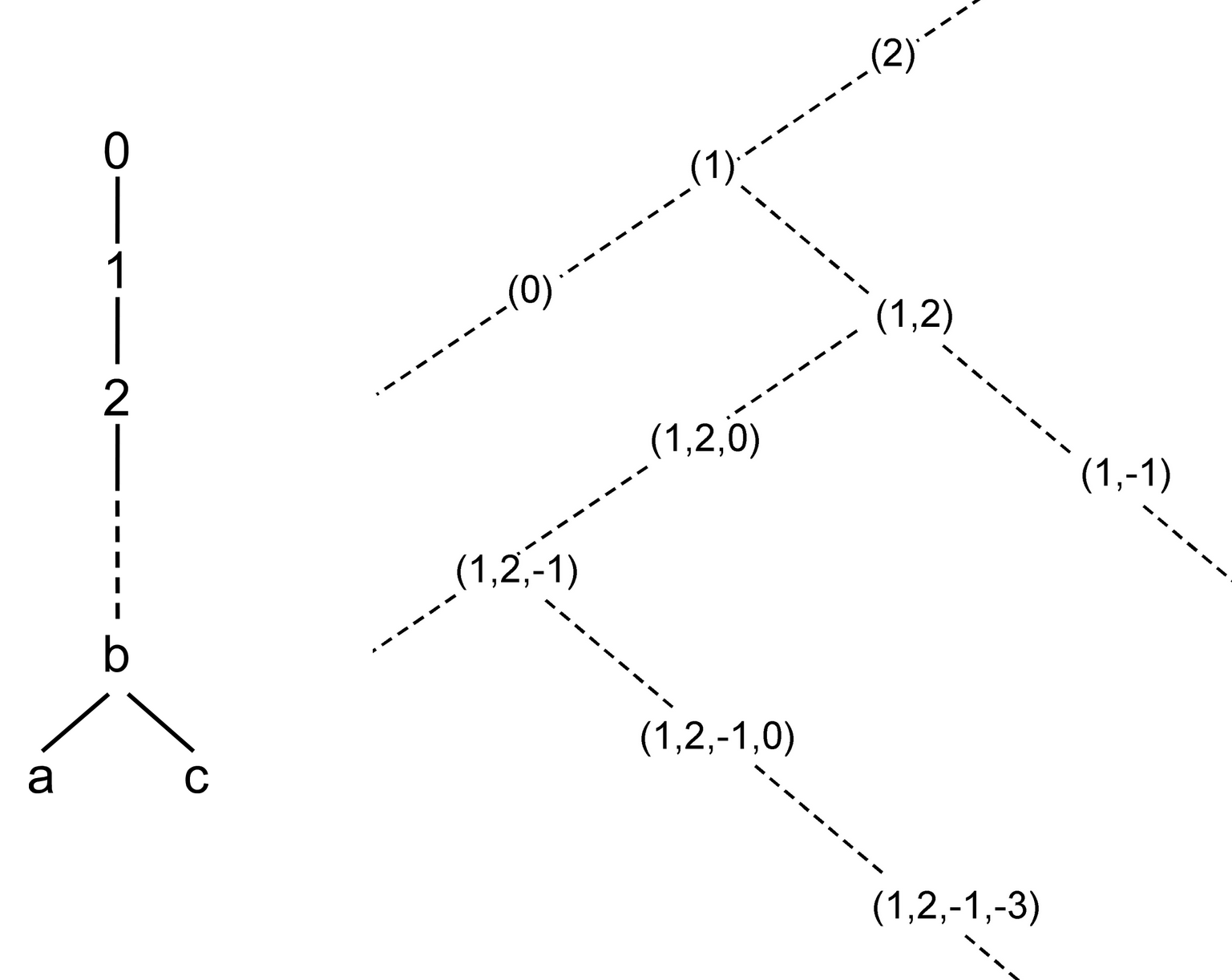
   Figure 1. The join-tree of Examples 1.2(3) and 3.4(a). A part of the universal O-tree of Example 1.2(4).

4. Fraïssé has defined in [12] (Section 10.5.3) a join-tree $T:=(Seq_{+}(\mathbb{Q}),\preceq)$ where $Seq_{+}(\mathbb{Q})$ is the set of finite nonempty sequences of rational numbers, such that every O-tree $(N,\leq)$ is isomorphic to $T[X]$ for some subset $X$ of $Seq_{+}(\mathbb{Q}).$ The strict partial order $\prec$ is defined as follows. For two sequences $\boldsymbol{x}=(x_{1},...,x_{n})$ and $\boldsymbol{y}=(y_{1},...,y_{m})$ we have $\boldsymbol{x}\prec\boldsymbol{y}$ if and only if:

         (i) $n\geq m$, $(x_{1},...,x_{m-1})=(y_{1},...,y_{m-1})$ and $x_{m}<y_{m},$ or

   (ii) $n>m$ and $(x_{1},...,x_{m})=(y_{1},...,y_{m}).$

   In particular, for all $x_{1},...,x_{n}$ and $z<x_{n}.$ we have $(x_{1},...,x_{n-1},z)\prec(x_{1},...,x_{n-1},x_{n})$ by (i) and $(x_{1},...,x_{n})\prec(x_{1},...,x_{n-1})$ by (ii). The strict partial order $\prec$ is generated by transitivity from these particular relations.

   Two sequences $\boldsymbol{x}$ and $\boldsymbol{y}$ as above are incomparable if and only if there is a sequence $(z_{1},...,z_{p})$ such that either $p\leq n$, $\boldsymbol{x}=(z_{1},...,z_{p-1},x_{p},...,x_{n}),z_{p}>x_{p}$, and $\boldsymbol{y}=(z_{1},...,z_{p-1},z_{p},y_{p+1},...,y_{m})$ or vice-versa by exchanging $\boldsymbol{x}$ and $\boldsymbol{y}$. Their join is $\boldsymbol{z}=(z_{1},...,z_{p}).$

   Examples of lines in $T$ are $\{(x)\mid x\in\mathbb{Q}\}$ and, for each $x_{1},x_{2}\in\mathbb{Q}$, the sets $\{(x_{1},x_{2},x)\mid x\in\mathbb{Q}\}$ and $\ \{(x_{1},x\,_{2},x),(x_{1},z),(y)\mid x,y,z\in\mathbb{Q},y\geq x_{1},z\geq x_{2}\}.$

   The right part of Figure 1 sketches some parts of this join-tree. We have $(1,-1)\prec$ $(1,2)\prec(2)$ and $(1,2,-1,0)\prec(1,2,0)$ by Case (i), and $(1,2,-1,-3)\prec(1,2,-1)\prec(1,2)\prec(1)$ by Case (ii).

   Examples of joins are $(0)\sqcup(1,2)=(1)$ (with $\boldsymbol{x}=(0)$, $\boldsymbol{y}=(1,2)$ and $\boldsymbol{z}=(1)$),

   and $(1,-1)\sqcup(1,2,-1,0)=(1,2)$ (with $\boldsymbol{x}=(1,-1)$, $\boldsymbol{y}=(1,2,-1,0)$ and $\boldsymbol{z}=(1,2)$).

   Examples of lines are $\{(1,2,x)\mid x\in\mathbb{Q}\},$ $\{(1,x)\mid x\in\mathbb{Q},x\geq 2\}$ and $\ \{(1,2,x),(1,z),(y)\mid x,y,z\in\mathbb{Q},y\geq 1,z\geq 2\}.$ We will also consider this tree in Examples 3.6 and 3.28.$\ \square$

Definitions 1.3 (The join-completion of an O-forest). Let  $J=(N,\leq)$ be an O-forest. We let $\mathcal{K}$ be the set of upwards closed lines $L_{\geq}(x,y)$ for all (possibly equal) nodes $x,y.\$If $x$ and $y$ have no upper-bound, then $L_{\geq}(x,y)$ is empty. If $x\sqcup y$ is defined, then $L_{\geq}(x,y)=L_{\geq}(x\sqcup y).$

The family $\mathcal{K}$ is countable. We let $j:N\rightarrow\mathcal{K}$ map $x$ to $L_{\geq}(x)$ and $\widehat{J}:=(\mathcal{K},\supseteq)$. We call $\widehat{J}$ the join-completion of $J$ because of the following proposition, stated with these hypotheses and notation.

Proposition 1.4. The partially ordered set $\widehat{J}:=(\mathcal{K},\supseteq)$ is a join-tree and $j$ is a join-embedding $J\rightarrow\widehat{J}$.

Proof Sketch.

We indicate the main steps. First, $\widehat{J}:=(\mathcal{K},\supseteq)$ is an O-tree: if $L,L^{\prime},L^{\prime\prime}\in\mathcal{K},L^{\prime}\subseteq L$ and $L^{\prime\prime}\subseteq L,$ then $L^{\prime}\subseteq L^{\prime\prime}$ or $L^{\prime\prime}\subseteq L^{\prime}$ because $L,L^{\prime},L^{\prime\prime}$ are upwards closed lines.

Claim: $\widehat{J}$ is a join-tree.

Proof : Let $L_{\geq}(x,y)$ and $L_{\geq}(z,u)$ be incomparable. We have $w\in L_{\geq}(x,y)-L_{\geq}(z,u)$ and $w^{\prime}\in L_{\geq}(z,u)-L_{\geq}(x,y).$ We claim that $L_{\geq}(w,w^{\prime})=L_{\geq}(x,y)\cap L_{\geq}(z,u),$ hence that it is the join of $L_{\geq}(x,y)$ and $L_{\geq}(z,u)$ in $\widehat{J}$. To prove the claim, we note that $L_{\geq}(w,w^{\prime})\subseteq L_{\geq}(w)\subseteq L_{\geq}(x,y)$ and similarly, $L_{\geq}(w,w^{\prime})\subseteq L_{\geq}(z,u)$, hence $L_{\geq}(w,w^{\prime})\subseteq L_{\geq}(x,y)\cap L_{\geq}(z,u).$ Conversely, assume we have $t\in(L_{\geq}(x,y)\cap L_{\geq}(z,u))-L_{\geq}(w,w^{\prime}).$ As $x\leq\{w,t\}$, we have $w\leq t$ or $t\leq w$. Assume $t\leq w$. Then since $t\in L_{\geq}(z,u),$ we have $w\in L_{\geq}(z,u)$, contradicting its definition. So we should have $w\leq t$ and similarly, $w^{\prime}\leq t$. Hence $t\in L_{\geq}(w,w^{\prime})$, contradicting its definition. This proves the claim. Note that $L_{\geq}(x,y)\cap L_{\geq}(z,u)=L_{\geq}(x,z).$ ∎

Then we have $x\leq y$ if and only if $L_{\geq}(y)\subseteq L_{\geq}(x)$, hence $j$ is an embedding. Since $L_{\geq}(x\sqcup y)=L_{\geq}(x)\cap L_{\geq}(y)$ that is the join of $L_{\geq}(x)$ and $L_{\geq}(y)$ in $\widehat{J}$, $j$ is a join-embedding. ∎

Its construction adds to $J$ the ”missing joins”. The existing joins are preserved. It follows that every O-forest $J$ with set of nodes $N$ is $T[N]$ for some join-tree $T$, in particular for $T:=\widehat{J}.$

1.4. Monadic second-order logic

We will express properties of relational structures by first-order (FO in short) and monadic second-order (MSO) formulas and sentences. Logical structures are relational (they have only relation symbols) and countable.

Definitions 1.5 (Quick review of terminology and notation). Monadic second-order logic extends first-order logic by the use of set variables $X,Y,Z$ … denoting subsets of the domain of the considered logical structure. The atomic formula $x\in X$ expresses the membership of $x$ in $X$. We call first-order a formula where set variables are not quantified. For example, a first-order formula can express that $X\subseteq Y$. A sentence is a formula without free variables.

A property $P$ of $\mathcal{R}$-structures where $\mathcal{R}$ is a finite set of relation symbols, is first-order or monadic second-order expressible (FO or MSO expressible) if it is equivalent to the validity, in every $\mathcal{R}$-structure $S$, of a first-order or monadic second-order sentence $\varphi$. The validity of $\varphi$ in $S$ is denoted by $S\models\varphi$. We say that a property of tuples of subsets $X_{1},...,X_{n}$ of the domains of structures in a class $\mathcal{C}$ is FO or MSO definable if it is equivalent to $S\models\varphi(X_{1},...,X_{n}$ ) in every $\mathcal{R}$-structure $S$ in $\mathcal{C}$, where $\varphi$ is a fixed FO or MSO formula with $n$ free set variables. A class of structures is FO or MSO definable or axiomatizable if it is characterized by an FO or MSO sentence.

Transitive closures and choices of sets, typically in graph coloring problems, are MSO but not FO expressible. See [11] for a detailed study of MSO expressible graph properties. Other comprehensive books are [14, 15].

Examples 1.6 (Partial orders and graphs).

1. A simple undirected graph $G$ can be identified with the {$edg$}-structure $(V_{G},edg_{G})$ where $V_{G}$ is its vertex set and $edg_{G}(x,y)$ means that there is an edge between $x$ and $y$ if $G$. For example, 3-colorability is expressed by the MSO sentence :

   $\exists X,Y[X\cap Y=\emptyset\wedge\lnot\exists u,v(edg(u,v)\wedge[(u\in X\wedge v\in X)\vee$

   $\qquad\qquad\qquad(u\in Y\wedge v\in Y)\wedge(u\notin X\cup Y\wedge v\notin X\cup Y)])].$

2. We now consider partial orders $(N,\leq)$. The FO formula $Lin(X)$ defined as $\forall x,y[(x\in X\wedge y\in X)\Longrightarrow(x\leq y\vee y\leq x)]$ expresses that a subset $X$ of $N$ is linearly ordered. The MSO formula

   $Lin(X)\wedge\exists a,b[Min(X,a)\wedge Max(X,b)\wedge\theta(X,a,b)]$

   expresses that $X$ is linearly ordered and finite, where $Min(X,a)$ and $Max(X,b)$ are FO formulas expressing respectively that $X$ has a least element $a$ and a largest one $b$, and $\theta(X,a,b)$ is an MSO formula expressing that :

   (i) each element $x$ of $X$ except $b$ has a successor $c$ in $X$ (i.e., $c$ is the least element of $L_{>}(x)\cap X$), and

   (ii) $(a,b)\in Suc^{\ast},$ where $Suc$ is the above defined successor relation (depending on $X$) and $Suc^{\ast}$ is its reflexive and transitive closure.

   Assertion (ii) is expressed by the MSO formula with free variables $a,b,X$ :

   $\forall U[U\subseteq X\wedge a\in U\wedge\forall x,y((x\in U\wedge(x,y)\in Suc)\Longrightarrow y\in U)\Longrightarrow b\in U].$

First-order formulas expressing $U\subseteq X$, $(x,y)\in Suc$ and Property (i) are easy to write. The finiteness of a linear order is not FO expressible. Without a linear order, the finiteness of a set $X$ is not MSO expressible.

Definitions 1.7 (Transformations of relational structures). As in [11], we call transduction a transformation of relational structures specified by logical formulas. We will try to be not too formal but nevertheless precise.

1. The basic type of transduction $\tau$ is as follows. A structure $S^{\prime}=(D^{\prime},R_{1}^{\prime},..,$ $R_{m}^{\prime})$ is defined from a structure $S=(D,R_{1},..,R_{n})$ and a $p$-tuple ($X_{1},..,X_{p})$ of subsets of $D$ called parameters by means of formulas $\chi,\delta,\theta_{R_{1}^{\prime}},...,\theta_{R_{m}^{\prime}}$ used as follows:

   $\tau(S,(X_{1},..,X_{p}))=S^{\prime}$ is defined if and only if $S\models\chi(X_{1},...,X_{p}),$

   $S^{\prime}=(D^{\prime},R_{1}^{\prime},..,R_{m}^{\prime})$ has domain $D^{\prime}\subseteq D$ such that $d\in D^{\prime}$ if and only if $S\models\delta(X_{1},...,X_{p},d),$

   $R_{i}^{\prime}$ is the set of tuples ($d_{1},...,d_{s})\in D^{\prime s}$, $s=\rho(R_{i}^{\prime})$, such that $S\models\theta_{R_{i}^{\prime}}(X_{1},\ldots,X_{n},d_{1},$ $\ldots,d_{s}).$

   We call $\tau$ an FO or an MSO transduction if the formulas that define it are, respectively, first-order or monadic second-order ones.

   As an example, the mapping from a graph $G=(V,edg)$ to the connected component $(V^{\prime},edg[V^{\prime}])$ containing a vertex $u$ is defined by $\chi,\delta$ and $\theta_{edg}$ where $\chi(X)$ expresses that $X$ is a singleton $\{u\}$, $\delta(X,d)$ expresses that there is a path between $d$ and the vertex in $X$, and $\theta_{edg}(x,y)$ is the formula always $\boldsymbol{true}$, say, $x=x$. It is an MSO transduction as path properties are expressible by monadic second-order formulas.

   
   

2. Transductions of the general type may enlarge the domain of the input structure. A structure $S^{\prime}=(D^{\prime},R_{1}^{\prime},..,R_{m}^{\prime})$ is defined from $S=(D,R_{1},..,R_{n})$ and a $p$-tuple ($X_{1},..,X_{p})$ of parameters as above by means of formulas $\chi,\delta_{1},...,\delta_{k}$ and others, $\theta_{R_{i}^{\prime},i_{1},...,i_{s}}$, used as follows:

   $\tau(S,(X_{1},..,X_{p}))=S^{\prime}$ is defined if and only if $S\models\chi(X_{1},...,X_{p}),$

   $S^{\prime}=(D^{\prime},R_{1}^{\prime},..,R_{m}^{\prime})$ has domain $D^{\prime}\subseteq(D\times\{1\})\uplus...\uplus(D\times\{k\})$ such that $(d,i)\in D^{\prime}$ if and only if $S\models\delta_{i}(X_{1},...,X_{p},d),$

   $R_{i}^{\prime}$ is the set of tuples (($d_{1},i_{1}),...,(d_{s},i_{s}))\in D^{\prime s}$, $s=\rho(R_{i}^{\prime})$, such that

   $\qquad\qquad\qquad S\models\theta_{R_{i}^{\prime},i_{1},...,i_{s}}(X_{1},...,X_{p},d_{1},...,d_{s}).$

   If $D$ is finite, then $\left|D^{\prime}\right|\leq k\left|D\right|$.

An easy example consists in the duplication of a graph $G=(V,edg)$ into the graph $H:=G\oplus G^{\prime}$, that is $G$ together with a disjoint copy $G^{\prime}$ of it. We get a graph $H$ up to isomorphism, because of the use of disjoint isomorphic copies. To define a transduction, we take $k=2$, $p=0$ (no parameter is needed), $\chi,\delta_{1},\delta_{2}$ always $\boldsymbol{true}$, $\theta_{edg,i,j}(x,y)$ always $\boldsymbol{false}$ if $i\neq j$, and equal to $edg(x,y)$ if $i=j$, where $i,j\in[2]$.

Another more complicated example is the transformation of an O-forest $J=(N,\leq)$ into its join-completion $\widehat{J}$. We define concretely the set of nodes of $\widehat{J}$ as ($N\times\{1\})\uplus(M\times\{2\})$ where $M$ is a subset of $N$ in bijection with the set of sets $L_{\geq}(x,y)$ such that $x$ and $y$ have no join, cf. Definition 1.3. This bijection can be made MSO definable, and so is the order relation of $\widehat{J}$. Defining $M$ is not straightforward because the sets $L_{\geq}(x,y)$ are not pairwise disjoint. We can use the notion of structuring of an O-tree: see Remark 3.35.

2. Quasi-trees and betweenness in O-trees

In this section, we define a betweenness relation in O-trees, and compare it with the betweenness relation induced by sets of nodes in join-trees or O-trees. We generalize the notion of quasi-tree defined and studied in [6] and [7].

For a ternary relation $B$ on a set $N$ and $x,y\in N$, we define $[x,y]_{B}:=\{x,y\}\cup\{z\in N\mid(x,z,y)\in B\}.$ If $n>2$, then the notation $\neq(x_{1},x_{2},...,x_{n})$ means that $x_{1},x_{2},...,x_{n}$ are pairwise distinct (hence abreviates an FO formula).

2.1. Betweenness in trees and quasi-trees

Definition 2.1 (Betweenness in linear orders and in trees).

1. Let $L=(X,\leq)$ be a linear order. Its betweenness relation $B_{L}$ is the ternary relation on $X$ defined by :

   $B_{L}(x,y,z):\Longleftrightarrow x<y<z$ or $z<y<x.\$

2. If $F$ is a forest, its betweenness relation $B_{F}$ is the ternary relation on $N_{F}$ defined by:

   $$B_{F}(x,y,z):\Longleftrightarrow x,y,z y x z$$ are pairwise distinct and is on a path between and .

   Such a path is unique if it does exist.

3. If $R=(N_{R},\leq_{R})$ is a rooted tree, we define its betweenness relation $B_{R}$ as $B_{\mathit{Und}(R)}$ where $\mathit{Und}(R)$ is the tree obtained from $R$ by forgetting its root.

For all $x,y,z\in N$, we have the following characterization of $B_{R}=B_{\mathit{Und}(R)}$:

$B_{R}(x,y,z)\Longleftrightarrow x,y,z$ are pairwise distinct, $x$ and $z$ have a join $x\sqcup_{R}z$ and $x<_{R}y\leq_{R}x\sqcup_{R}z$ or $z<_{R}y\leq_{R}x\sqcup_{R}z$.

It follows that the betweenness relation of a rooted tree is invariant under a change of root: $B_{R}=B_{R^{\prime}}$ if $\mathit{Und}(R)=\mathit{Und}(R^{\prime})$.

Example 2.2. Figure 2 shows a rooted tree $R$ with root 0. For illustrating the above description of $B_{R}$, we note that $B_{R}(b,a,0)$ and $b<a<0=b\sqcup 0$, and also that $B_{R}(b,a,c)$ and $b<a<1=b\sqcup c.$ The betweenness of the partial order $(N_{R},\leq_{R})$ in the sense of [9, 16] does not contain the triple $(b,a,c)$. It is only the union of those of the four paths from the leaves $b,d,f,h$ to the root 0.

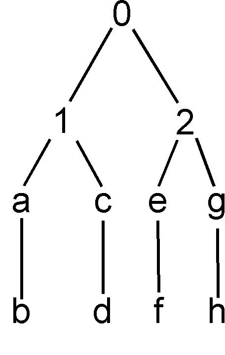
Figure 2. The rooted tree $R$ of Example 2.2.

With a ternary relation $B$ on a set $X$, we associate the ternary relation $A$ on $X$ : $A(x,y,z):\Longleftrightarrow B(x,y,z)\vee B(x,z,y)\vee B(y,x,z)$, to be read : $x,y,z$ are aligned. If $n\geq 3$, then $B^{+}(x_{1},x_{2},...,x_{n})$ stands for the conjunction of the conditions $B(x_{i},x_{j},x_{k})$ for all $1\leq i<j<k\leq n.$ They imply that $x_{1},x_{2},...,x_{n}$ are pairwise distinct.

The following is Proposition 5.2 in [7] or Proposition 9.1 in [11].

Proposition 2.3.

1. The betweenness relation $B$ of a linear order $(X,\leq)$ satisfies the following properties for all $x,y,z,u\in X$.

   A1 : $B(x,y,z)\Rightarrow\neq(x,y,z).$

   A2 : $B(x,y,z)\Rightarrow B(z,y,x).$

   A3 : $B(x,y,z)\Rightarrow\lnot B(x,z,y).$

   A4 : $B(x,y,z)\wedge B(y,z,u)\Rightarrow B^{+}(x,y,z,u).$

   A5 : $B(x,y,z)\wedge B(x,u,y)\Rightarrow B^{+}(x,u,y,z).$

   A6 : $B(x,y,z)\wedge B(x,u,z)\Rightarrow y=u\vee B^{+}(x,u,y,z)\vee B^{+}(x,y,u,z).$

   A7’ : $\neq(x,y,z)\Rightarrow A(x,y,z).$

2. The betweenness relation $B$ of a tree $T$ satisfies the properties A1-A6 for all $x,y,z,u$ in $N_{T}$ together with the following weakening of A7’:

   A7 : $\neq(x,y,z)\Rightarrow A(x,y,z)\vee\exists w[B(x,w,y)\wedge B(y,w,z)\wedge B(x,w,z)].$

Remarks 2.4.

1. Property A4 could be written equivalently : $B(x,y,z)\wedge B(y,z,u)\Rightarrow B(x,y,u)\wedge B(x,z,u).$ Property A5 could be written $B(x,y,z)\wedge B(x,u,y)\Rightarrow B(x,u,z)\wedge B(u,y,z).$

2. Property A7’ says that if $x,y,z$ are three elements in a linear order, then, one of them is between the two others. Properties A1-A5 belong to the axiomatization of betweenness in partial orders given in [9, 16]. Property A6 is actually a consequence of Properties A1-A5 and A7’, as one proves easily.

3. Property A7 says that, in a tree $T$, if $x,y,z$ are three nodes not on a same path, some node $w$ is between any two of them. In this case, we have :

   $\{w\}=P_{x,y}\cap P_{y,z}\cap P_{x,z}$ where $P_{x,y}$ is the set of nodes on the path between $x$ and $y$,

   so that we have $B(x,w,y)\wedge B(y,w,z)\wedge B(x,w,z)$.

   If $T$ is a rooted tree, and $x,y,z$ are not on a path from a leaf to the root, then $w$ is the join (the least common ancestor) of two nodes among $x,y,z$. In the rooted tree $R$ of Figure 2, if $x\ =a,y=d$ and $z=e$, we have $w=1=x\sqcup y$.

   Property A6 is a consequence of Properties A1-A5 and A7.

4. Properties A1-A6 (for an arbitrary structure $S=(N,B)$) imply that the two cases of the conclusion of A7 are exclusive and that, in the second one, there is a unique node $w$ satisfying $B(x,w,y)\wedge B(y,w,z)\wedge B(x,w,z)$ (by Lemma 11 of [6]), that is denoted by $M_{S}(x,y,z)$.

Convention

The letter $B$ and its variants, $B_{T},B_{1}$, etc. will always denote ternary relations. We will only consider ternary relations satisfying Properties A1 and A2. In other words, we will consider $B(x,y,z)$ as identical to $B(z,y,x)$ and $\neq(x,y,z)$ as an immediate consequence of $B(x,y,z).$ This is similar to the standard usage of considering $x=y$ as identical to $y=x$ and $x\neq y$ as an immediate consequence of $x<y.$ It follows that $B^{+}(x_{1},x_{2},...,x_{n})$ stands also for the conjunction of the conditions $B(x_{k},x_{j},x_{i})$ for $1\leq i<j<k\leq n.$ In the proofs and discussions about structures $(N,B)$, we will not make explicit the uses of A1 and A2 .

Definitions 2.5 (Another betweenness property). We define the following property of a structure $S=(N,B)$:

A8 : $\forall u,x,y,z[\neq(u,x,y,z)\wedge B(x,y,z)\wedge\lnot A(y,z,u)\Rightarrow B(x,y,u)]$.

Example and Remark 2.6.

1. Properties A1-A6 do not imply A8. Consider $S:=([5],B)$ where $B$ satisfies (only) $B^{+}(1,2,3,4)\wedge B(4,3,5)$ illustrated in Figure 3. (There is no curve line going through 1,2,5 because $B(1,2,5)$ is not assumed to be valid). Conditions A1-A6 hold but A8 does not, because we have $\lnot A(2,3,5)\wedge B(1,2,3)$. Then, A8 would imply $B(1,2,5)$ that is not assumed.

2. Properties A1-A5 and A8 imply A6. Assume we have $B(x,y,z)\wedge B(x,u,z)\wedge y\neq u$.  

   If $\lnot A(y,z,u),$ we have $B(x,y,u)$ by A8 and then $B^{+}(x,y,u,z)$ by A5, which implies $B(y,u,z)$ and $A(y,z,u)$ by the definitions, which contradicts the assumption.

   Hence, we have $A(y,z,u),$ that is, $B(y,z,u)$ or $B(z,y,u)$ or $B(y,u,z)$. If $B(y,z,u)$ holds, then we have  $B^{+}(x,y,z,u)$ by A4, hence $B(x,z,u)$ which contradicts $B(x,u,z)$ by A3. If $B(z,y,u)$ holds, we have  $B^{+}(x,u,y,z)$ by A5 (since $B(x,u,z)$ holds), that is one case of the desired conclusion. The last case is $B(y,u,z),$ that yields by A5 (since $B(x,y,z)$ holds) the other case of the conclusion. We will keep Property A6 in our axiomatization for its clarity and to shorten proofs. ∎

   

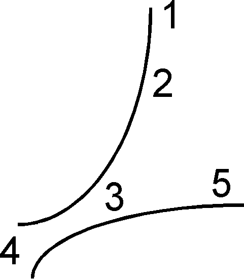
   Figure 3. Structure $S$ of Example 2.6(1)

We say that $(N,B)$ is trivial if $B=\emptyset$. In this case, Properties A1-A6, and A8 hold.

Lemma 2.7. Let $S=(N,B)$ satisfy A1-A6.

1. A7 implies A8.

2. If A8 holds, then the Gaifman graph of $S$ is either edgeless (if $B=\emptyset$) or connected.

Proof.

1. Let us assume $\neq(u,x,y,z)\wedge B(x,y,z)\wedge\lnot A(u,y,z)$ and prove $B(x,y,u).$ There is $w$ such that $B(u,w,y)\wedge B(y,w,z)\wedge B(u,w,z).$ From $B(x,y,z)$, we get $B^{+}(x,y,w,z)$ by A5, hence, $B(x,y,w)$ by the definitions. Then, from $B(y,w,u)$ and  $B(x,y,w),$ we get $B^{+}(x,y,w,u)$ by A4, whence $B(x,y,u)$ by the definitions, as desired.

2. Assume that the Gaifman graph $\mathit{Gf}(S)$ is not edgeless. We have $B(x,y,z)$ for some $x,y,z$. Consider $u$ different from them. Either $A(y,z,u)\$or $B(x,y,u)$ (or both) hold by A8. Hence, $u$ is in the same connected component as $x,y,z$. ∎

Definition 2.8 (Quasi-trees and betweenness in join-trees [6]).

1. A quasi-tree is a structure $S=(N,B)$ such that $B$ is a ternary relation on a set $N$, called the set of nodes, that satisfies conditions A1-A7. To avoid uninteresting special cases, we also require that $\left|N\right|\geq$3. We say that $S$ is discrete if $[x,y]_{B}:=\{x,y\}\cup\{z\in N\mid B(x,z,y\}$ is finite for all $x,y$.

2. From a join-tree $J=(N,\leq),$ we define a ternary relation $B_{J}$ on $N$ by :

   $B_{J}(x,y,z):\Longleftrightarrow\neq(x,y,z)\wedge([x<y\leq x\sqcup z]\vee[z<y\leq x\sqcup z]),$

   called its betweenness relation. As a definition, we use here the observation made for rooted trees in Definition 2.1(c). The join $x\sqcup z$ is always defined.

3. In a quasi-tree $S=(N,B)$, we define the path that links $x$ and $y$ as the set $[x,y]_{B}$. It is linearly ordered with least element $x$ and largest one $y$ in such a way that $u<v$ if and only if $x=u\wedge y=v$ or $B(x,u,v)$ or $B(u,v,y)$. An element may have no successor or no predecessor (hence it may not be a path in the usual sense). However, this set is connected in the Gaifman graph $\mathit{Gf}(S)$.

Figure 4 shows a quasi-tree, where the dashed lines represent infinite paths in the above sense. In such a structure, no adjacency notion is available. The ternary relation of betweenness replaces it.

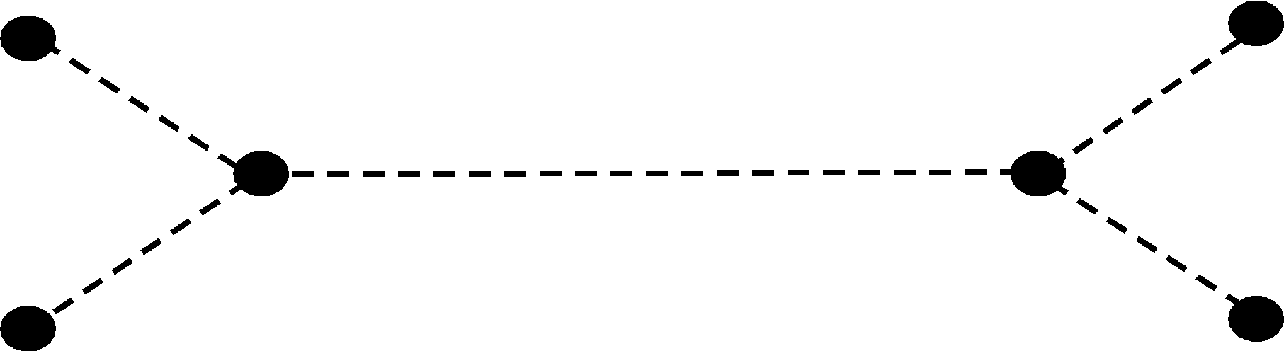
Figure 4. A quasi-tree.

The following theorem is Proposition 5.6 of [7].

Theorem 2.9.

1. The structure $\mathit{qt}(J):=(N,B_{J})$ associated with a join-tree $J=(N,\leq)$ with at least 3 nodes is a quasi-tree. Conversely, every quasi-tree $S$ is $\mathit{qt}(J)$ for some join-tree $J$.

2. A quasi-tree is discrete if and only if it is $\mathit{qt}(J)$ for the join-tree $J:=(N_{R},\leq_{R})$ where $R$ is a rooted tree.

This theorem shows that one can specify a quasi-tree by a binary relation, actually a partial order. However, this is inconvenient because choosing a partial order breaks the symmetry. This motivates our use of a ternary relation. Similarily, betweenness can formalize the notion of a linear order, up to reversal.

2.2. Other betweenness structures

Definition 2.10 (Induced betweenness in a quasi-tree). If $Q=(N,B)$ is a quasi-tree, $X\subseteq N$, we say that $Q[X]:=(X,B[X])$ is an induced betweenness relation in $Q$. It is induced on $X$.

Remark and example 2.11. The structure $Q[X]$ need not be a quasi-tree because A7 does not hold for a triple $(x,y,z)\in X^{3}$ such that $M_{Q}(x,y,z)$ is not in $X$ (cf. Proposition 2.3).

Figure 5 shows a tree $T$ to the left with $N_{T}=[7]$. Its betweenness relation $B_{T}$ is expressed in a short way by the properties $B_{T}^{+}(1,2,7,3,4)$, $B_{T}^{+}(1,2,7,5,6)$ and $B_{T}^{+}(6,5,7,3,4).$ Let $Q:=(N_{T},B_{T})$ and $N_{1}:=[6].$ The induced betweenness $S_{1}:=Q[N_{1}]$ is illustrated on the right, where the curve lines represent the facts $B_{T}^{+}(1,2,3,4)$, $B_{T}^{+}(1,2,5,6)$ and $B_{T}^{+}(6,5,3,4).$ It is not a quasi-tree because $7=M_{Q}(1,4,6)$ is not in $N_{1}$.$\square$

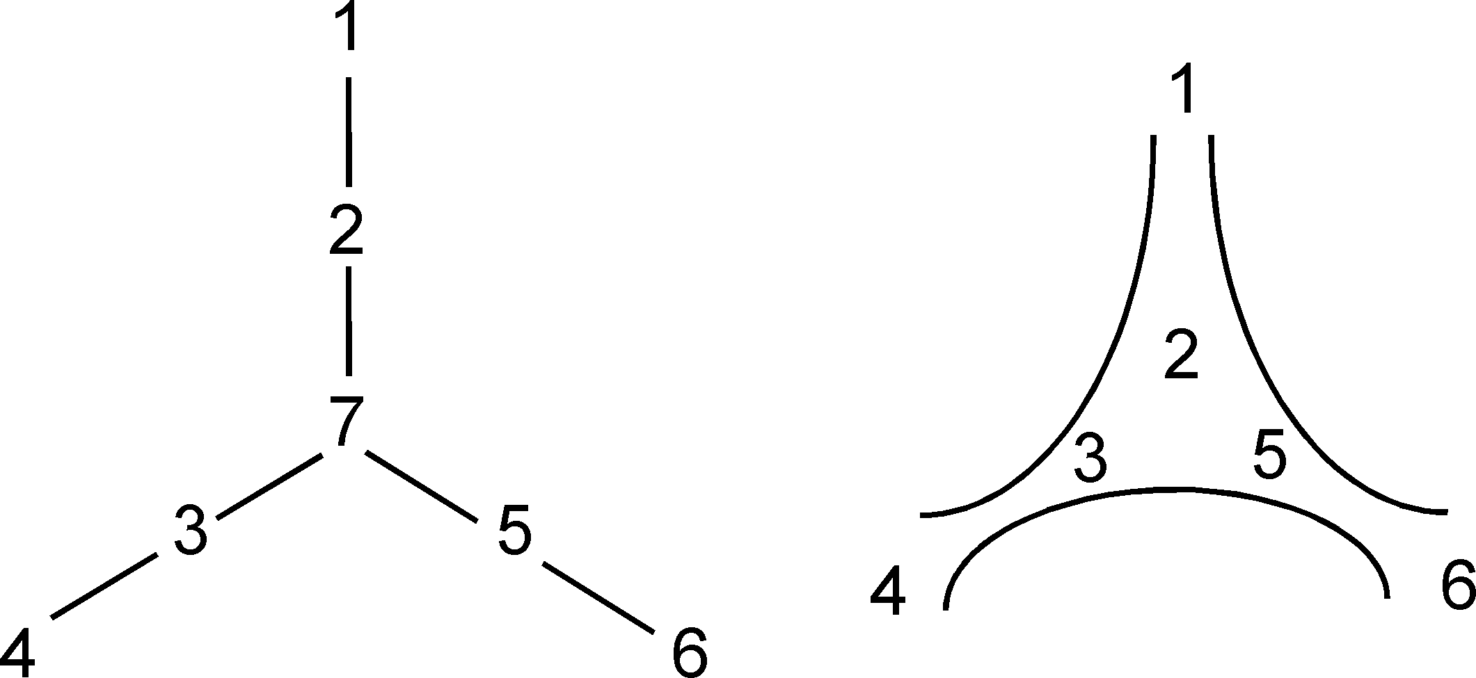
Figure 5. An induced betweenness in a quasi-tree, cf. Example 2.11.

Our objective is to axiomatize induced betweenness relations in quasi-trees (equivalently in join-trees), similarly as betweenness relations in join-trees are by A1-A7 in Theorem 2.9(1).

Proposition 2.12. An induced betweenness relation in a quasi-tree satisfies properties A1-A6 and A8.

Proof.

The FO sentences expressing A1-A6 and A8 are universal, that is, are of the form $\forall x,y,...,z.\varphi(x,y,...,z)$ where $\varphi$ is quantifier-free. The validity of such sentences is preserved under taking induced substructures (we are dealing with relational structures). The result follows from Theorem 2.9 and Lemma 2.7(1) showing that a quasi-tree satisfies A8. ∎

Our objective is to prove that a ternary relation is an induced betweenness in a quasi-tree if and only if it satisfies Properties A1-A6 and A8. Our proof will use O-trees.

Figure 6 illustrates Property A8 which says: $B(x,y,z)\wedge\lnot A(y,z,u)\Rightarrow B(x,y,u).$ The white circle between $y$ and $z$ represents the node $M_{Q}(y,z,u)$ of a quasi-tree $Q$ that has been deleted, so that Property A7 does not hold in the structure $Q[N-\{M_{Q}(y,z,u)\}]$.

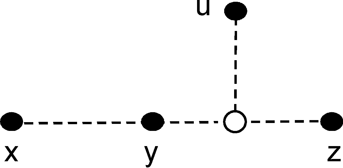
Figure 6. Illustration of Property A8.

Definition 2.13 (Betweenness in O-forests).

1. The betweenness relation of an O-forest $F=(N,\leq)$ is the ternary relation $B_{F}$ on $N$ such that :

   $B_{F}(x,y,z):\Longleftrightarrow\neq(x,y,z)\wedge[(x<y\leq x\sqcup z)\vee(z<y\leq x\sqcup z)].$

   The validity of the right handside needs that $x\sqcup z$ be defined.

2. If $F=(N,\leq)$ is an O-forest and $X\subseteq N$, then $B_{F}[X]$ is an induced betweenness relation in $F$ and $(X,B_{F}[X])$ is an induced betweenness structure.

   The difference with Definition 2.8(b) is that if $x$ and $z$ have no least upper-bound (i.e., if $x\sqcup z$ is undefined, which implies that $x$ and $z$ are incomparable, denoted by $x\bot z$), then $B_{F}$ contains no triple of the form $(x,y,z).$

   If $F$ is a finite O-tree, it is a join-tree and thus, $(N,B_{F})$ is a quasi-tree.$\square$

We have four classes of betweenness structures $S=(N,B)$ : quasi-trees, induced betweenness structures in quasi-trees, betweenness and induced betweenness structures in O-forests, denoted respectively by QT, IBQT, BO and IBO.

Remarks 2.14.

1. Let $T$ be a tree and $X$ a set of leaves. The induced betweenness relation $B_{T}[X]$ is trivial.

2. The Gaifman graph of a betweenness structure $S$ is connected in the following cases : $S\in$IBQT and is not trivial or $S$ is the betweenness structure of an O-tree. It may be not connected in the other cases.

3. If $S$ is an induced betweenness in an O-forest consisting of several disjoint O-trees, then two nodes in the different O-trees cannot belong to a same triple. It follows that they cannot be linked by a path in the graph $\mathit{Gf}(S)$. Hence, a structure $(N,B)$ is the betweenness of an O-forest, or an induced betweenness in an O-forest if and only if each of its connected components is so in an O-tree. We will only consider betweenness of O-trees (class BO) and induced betweenness in O-trees (class IBO).

Proposition 2.15. We have the following proper inclusions:

QT $\subset$ IBQT $\cap$ BO, IBQT$\ \subset$ IBO and BO $\subset$ IBO.

The classes IBQT and BO are incomparable. For finite structures, we have QT $=$ BO.

These inclusions are illustrated in Figure 7. Structures $S_{1},S_{2},S_{4}$ and $S_{5}$ witnessing proper inclusions are described in the proof.

Proof.

All inclusions are clear from the definitions. We give examples to prove that the inclusions are proper. We recall that $S[X]:=(X,B[X])$ if $S=(N,B)$ and $X\subseteq N$.

1. The structure $S_{1}$ of Example 2.11, shown in the right part of Figure 5, is in IBQT but not in QT. It is not in BO either, because otherwise, it would be a quasi-tree as it is finite.

   

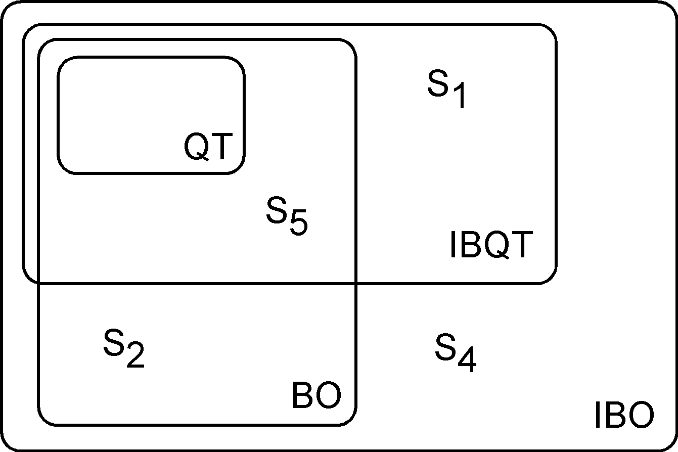
   Figure 7. Proper inclusions of classes proved in Proposition 2.15.

   

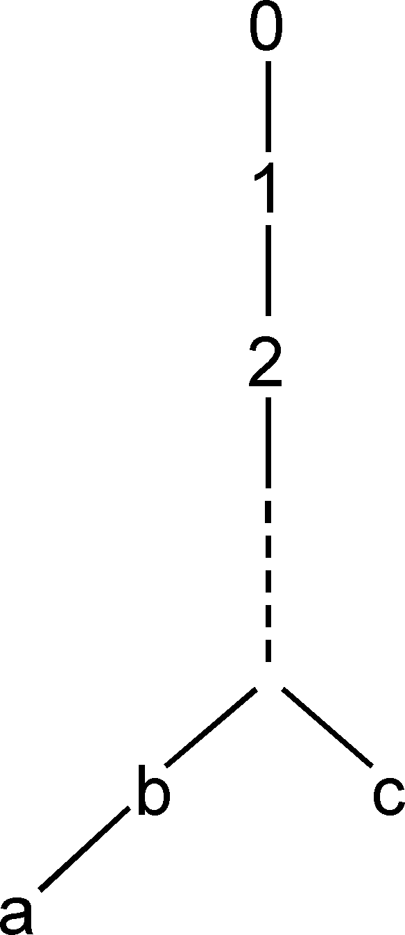
   Figure 8. The O-tree $T_{2}$ used in the proof of Proposition 2.15, Parts (2) and (4).

2. We consider $N_{2}:=\mathbb{N}\cup\{a,b,c\}$ and the O-tree $T_{2}:=(N_{2},\preceq)$ in Figure 8 such that $a\prec b\prec i\prec j$ and $c\prec i\prec j$ for all $i,j$ in $\mathbb{N}$ such that $j<i$. Its betweenness structure $S_{2}:=(N_{2},B_{2})$ is described by the properties $B_{2}^{+}(a,b,i,j,k)$ and $B_{2}^{+}(c,i,j,k)$ for all $i,j,k$ in $\mathbb{N}$ such that $k<j<i$. Since $b$ and $c$ have no least upper-bound in $T_{2}$, we do not have $B_{T_{2}}(a,b,c)$. Hence, $S_{2}$ is in BO but not in IBQT, as it does not satisfy A8: we have $\lnot A_{T_{2}}(0,b,c)\wedge B_{T_{2}}(a,b,0)$ but not $B_{T_{2}}(a,b,c)$. The classes IBQT and BO are incomparable.

   If we take $c$ as new root, we obtain a join-tree $U=(N_{2},\preceq^{\prime})$ where $a\prec^{\prime}b\prec^{\prime}c$ and $0\prec^{\prime}1\prec^{\prime}2...\prec^{\prime}i\prec^{\prime}...\prec^{\prime}c.$ and $\{a,b\}\bot^{\prime}\mathbb{N}$. Clearly $B_{U}\neq B_{T_{2}}$.

   Hence, betweenness in O-trees depends on some kind of orientation, that can be specified either by a root or by an upwards closed line (cf. the notion of structuring in Definition 3.27 below). To the opposite, in the case of quasi-trees and induced betweenness in quasi-trees, any node can be taken as root in the constructions of the relevant join-trees (cf. [7] for quasi-trees, and the proof of Theorem 3.1 and Remark 3.4(d) for induced betweenness in quasi-trees).

   
   

3. To prove that the inclusion of BO in IBO is proper, we consider $S_{3}:=(N_{3},B_{T_{3}}),N_{3}:=\{a,b,c,d\}\cup\mathbb{Q}$ and the O-tree $T_{3}:=(N_{3},\prec)$ ordered such that:

   - $a\prec b\prec i\prec j$ and $d\prec c\prec i\prec j$ for all $i,j\in\mathbb{Q}$ such that $\sqrt{2}<i<j,$ and

   - $i\prec j$ if $i,j\in\mathbb{Q}$, $i<j.$

   It is shown in Figure 9(a). The upper dotted line is isomorphic to $\mathbb{Q}_{>}(\sqrt{2}):=\{i\in\mathbb{Q\mid}i>\sqrt{2}\}$ and the lower one is isomorphic to $\mathbb{Q}_{<}(\sqrt{2}):=\mathbb{Q}-\mathbb{Q}_{>}(\sqrt{2})$.

   We let then $S_{4}:=S_{3}[\{a,b,c,d,1,2,3\}]$ with corresponding O-tree $T_{4}$ (Figure 9(b)). The structure $S_{4}$ is in IBO but not in BO. Otherwise, as it is finite, it would be a quasi-tree. But $S_{4}$ does not satisfy A8 : we have $B_{T_{3}}(a,b,3)\wedge\lnot A_{T_{3}}(b,c,3)$ but $(a,b,c)\notin B_{T_{3}}$. For this reason, $S_{4}$ is not in IBQT either.

   Note that $S_{4}$ in IBO is finite but is not the induced betweenness relation of a finite O-tree. Otherwise, it would be in IBQT because a finite O-tree is a join-tree.

   

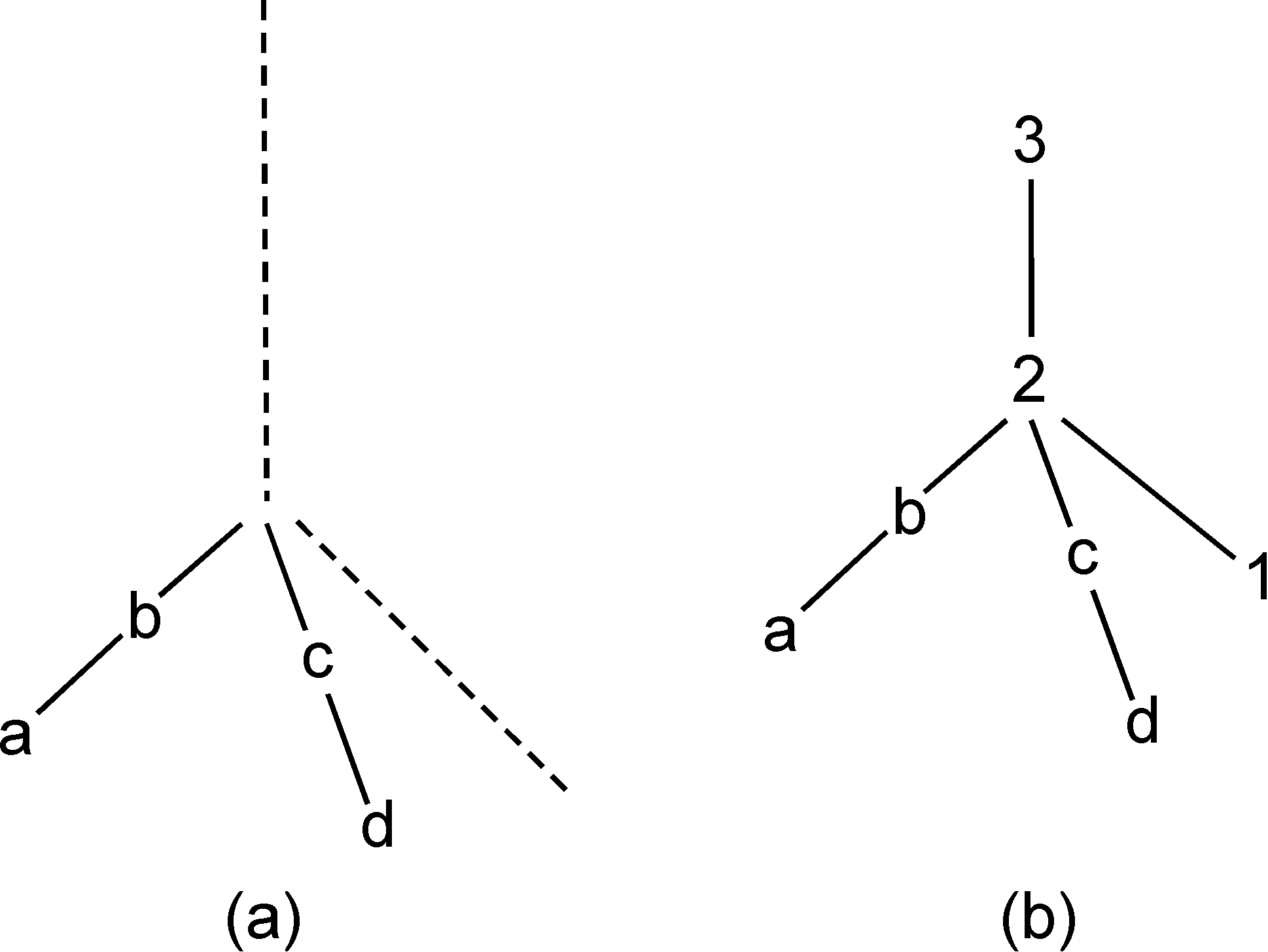
   Figure 9. Part (a) shows $T_{3}$ and (b) shows $T_{4}$ of the proof of Proposition 2.15, Part (3), and Example (3.6).

4. Let $T_{5}$ be the O-tree $T_{2}[N_{5}]$ where $N_{5}:=\mathbb{N}\cup\{b,c\}$ and $S_{5}:=(N_{5},B_{T_{5}}).$ (Figure 8 shows $T_{2}$). Then $S_{5}$ is in BO, and also in IBQT : just add to $T_{5}$ a least upper-bound $m$ for $b$ and $c$ such that $m<\mathbb{N}$, one obtains a join-tree. It is not a quasi-tree because A7 does not hold for the triple $(b,c,3)$ (relative to $B_{5}$). Hence, we have QT $\subset$ IBQT$\cap$BO.

   Note that $S_{2}$ is not in IBQT but its induced substructure $S_{5}\$is. ∎

Figure 7 shows how these examples are located in the different classes of betweenness relations. The structures $S_{1}$ and $S_{4}$ are finite, $S_{2}$ and $S_{5}$ are infinite, which is necessary because the finite structures in BO and QT are the same.

Remark 2.16. An alternative betweenness relation for an O-forest $F=(N,\leq)$ could be defined by $B_{F}^{\prime}:=B_{\widehat{F}}[N]$ (see Definition 1.3 for $\widehat{F}$). If $F$ is an O-tree, we have $(x,y,z)\in B_{F}^{\prime}$ if and only if $\neq(x,y,z)$ and, either $x<y\leq m\geq z$ or $z<y\leq m\geq x$ for some $m$ that need not be the join in $F$ of $x$ and $z$. As $(N,B_{F}^{\prime})$ is an induced betweenness in a join-tree, this definition does not bring anything new.

3. Axiomatizations

3.1. First-order axiomatizations

Our first main result is Theorem 3.1 that provides a first-order axiomatization of the class IBQT, among countable (finite or countably infinite) structures.

All our constructions are relative to countable structures. The letter $B$ will always denote ternary relations. Writing $(x,y,z)\in B$ is equivalent to stating that $B(x,y,z)$ holds.

3.1.1. Induced betweenness in quasi-trees

Theorem 3.1. The class IBQT is axiomatized by the first-order properties A1-A6 and A8.

With $S=(N,B)$ and $r\in N,$ we associate the binary relation $\leq_{r}$ on $N$ such that $x\leq_{r}y:\Longleftrightarrow x=y\vee y=r\vee B(x,y,r).$

Lemma 3.2. Let $S=(N,B)$ satisfy Axioms A1-A6 and $r\in N.$ Then :

(1) $T(S,r):=(N,\leq_{r})$ is an O-tree,

(2) if $x<_{r}y<_{r}z$, then $(x,y,z)\in B$,

(3) if $(x,y,z)\in B$, $x<_{r}y$ and $z<_{r}y$, then $y=x\sqcup_{r}z$,

(4) if $x<_{r}w<_{r}y$ and $z<_{r}w$, then $(x,y,z)\notin B$.

Proof.

1. The relation $\leq_{r}$ is a partial order: antisymmetry follows from A3 and transitivity from A5. The node $r$ is its largest element. Axiom A6 implies that, for any $x\in N$, the set $L_{\geq_{r}}(x)$ is linearly ordered. Hence, $T(S,r):=(N,\leq_{r})$ is an O-tree with root $r$.

2. This is clear if $z=r$ and follows from A5 otherwise.

3. Assume that $B(x,y,z)$ holds $x<_{r}y$ and $z<_{r}y$. We cannot have $x<_{r}z$ or $z<_{r}x$ because otherwise, we have by (2) $B(x,z,y)$ or $B(z,x,y),$ contradicting $B(x,y,z)$ by A3.

   Assume for a contradiction, that $x<_{r}w<_{r}y$ and $z<_{r}w<_{r}y.$ Then, by (2), we have $B(x,w,y)$ and $B(z,w,y).$ We get $B^{+}(x,w,y,z)$ by A5, which gives $B(w,y,z)$, contradicting A3 since we have $B(z,w,y).$

4. From $x<_{r}w<_{r}y$ we get $B(x,w,y)$ by (2). With $B(x,y,z)$, A5 gives $B^{+}(x,w,y,z)$, whence $B(w,y,z)$ by the definitions. From $z<_{r}w<_{r}y,$ we get $B(z,w,y)$ by (2), which is incompatible with $B(w,y,z)$ by A3. ∎

Lemma 3.3. Let $S:=(N,B)$ satisfy A1-A6 and A8, and $r\in N$.

1. Let $x$ and $y$ be incomparable with respect to $\leq_{r}$. If $z<_{r}y$, then $(x,y,z)\in B$.

2. If $(x,y,z)\in B$, then $x<_{r}y$ or $z<_{r}y$.

3. We have $B\subseteq B_{T(S,r)}$ if $N$ is finite.

Proof.

In this proof, $<$, $\leq$ and $\sqcup$ will denote $<_{r},\leq_{r}$ and $\sqcup_{r}.$

1. Let $x$ and $y$ are incomparable and $z<y$. The root $r$ is not any of $x,y,z.$ If $B(x,r,y)$ holds, then, from $B(r,y,z)$ we have $B^{+}(x,r,y,z)$ by A4, whence $B(x,y,z)$. Otherwise, $A(x,y,r)$ does not hold, and as we have $B(z,y,r)$, we get by A8 $B(z,y,x),$ i.e.,$B(x,y,z)$.

2. Let $(x,y,z)\in B$. We have several cases.

   Case 1 : $x$ or $z$ is $r$. We get respectively $z<y$ or $x<y$.

   Case 2: $y=r$. Then $z<y$ and $x<y$.

   Case 3: $\neq(x,y,z,r)$ and $\lnot(A(y,z,r)$. We have $B(x,y,r)$ by A8, hence, $x<y$.

   Case 4: $\neq(x,y,z,r)$ and $A(y,z,r)$ holds. If $B(y,z,r),$ we have $B^{+}(x,y,z,r)$ by A4, hence, $x<y$. If $B(y,r,z),$ we have $B^{+}(x,y,r,z)$ by A5, hence, $x<y$. If $B(r,y,z),$ we have $z<y$.

3. Let $(x,y,z)\in B$. We have $x<y$ or $z<y$ by (2). As $N$ is finite, $x$ and $z$ have a join $x\sqcup z$ in the rooted tree $T(S,r)$.  Assume $x<y.$ If $y\leq x\sqcup z$, we have $(x,y,z)\in B_{T(S,r)}$ by Definition 2.13, as desired. Otherwise, $x\sqcup z<y$, hence $x\leq x\sqcup z<y$. We cannot have $x\sqcup z=z$ because then $(x,z,y)\in B$ by lemma 3.2(2), contradicting $(x,y,z)\in B$ (by A3). Hence, $x\bot z$ and then $x<x\sqcup z<y$ and $z<x\sqcup z<y$. Lemma 3.2(3) yields $y=x\sqcup z$, contradicting the assumption. Hence, we have $(x,y,z)\in B_{T(S,r)}$. The case $z<y$ is similar. ∎

Examples 3.4.

1. In statement (3) above, we may have a proper inclusion. Consider $S_{6}$ defined as $(N_{6},B_{6})$ with $N_{6}:=\{0,1,2,a,c\}$, $B_{6}^{+}(0,1,2,a)$, $B_{6}^{+}(0,1,2,c)$ and $r:=0$. Then $T(S_{6},0)=T[N_{6}]$ where $T$ is the join-tree at the left of Figure 1.  We have $(a,2,c)$ in $B_{T(S_{6},0)}$ but not in $B_{6}$.

2. The inclusion $B\subseteq B_{T(S,r)}$ may be false if $S$ is infinite.  Consider $S_{7}=(\mathbb{N}\cup\{a,b,c\},B_{7})$ defined from $S_{2}=(\mathbb{N}\cup\{a,b,c\},B_{2})$ in the proof of Proposition 2.15 (see Figure 8), where $B_{7}:=B_{2}\cup\{(a,b,c),(c,b,a)\}$. Then $T(S_{7},0)=T_{2}$ of this proof, but $(a,b,c)\notin B_{T(S_{7},0)}.$

3. We give an example showing how we will prove Theorem 3.1. Let $S_{8}:=(N_{8},B_{8})$ such that $N_{8}:=\{0,a,b,c,d,e,f,g,h\}$ and $B_{8}$ is defined by the following properties :

   (i) $B_{8}^{+}(b,a,c,d)$, $B_{8}^{+}(f,e,g,h)$,

   (ii) $B_{8}^{+}(b,a,0,e,f)$, $B_{8}^{+}(d,c,0,e,f)$, $B_{8}^{+}(b,a,0,g,h)$, $B_{8}^{+}(d,c,0,g,h)$.

   Figure 10(a) shows this structure drawn with the conventions of Figures 3 and 5 (right part). It shows properties $B_{8}(b,a,0)$, $B_{8}(d,c,0)$, $B_{8}(e,f,0)$ and $B_{8}(g,h,0)$. It does not show the four conditions of type (ii) for the purpose of clarity. We have neither $B_{8}^{+}(b,a,0,c,d)$ nor $B_{8}^{+}(e,f,0,g,h)$.

   By adding new nodes $1$ and 2 to $T(S_{8},0)$ such that $a<1<0,c<1<0,e<2<0$ and $g<2<0,$ we get the rooted tree $T_{8}$ of Figure 10(b).  Then $B_{7}=B_{T_{8}}[N_{7}]$, hence, is in IBQT.

   The proof of Theorem 3.1 will consist in adding new elements to trees $T(S,r)$ for such cases.

4. Let $S=(N,B)$ satisfies A1-A7 (and thus A8 by Lemma 2.7). For each $r\in N$, the O-tree $T(S,r)$ is a join-tree and $B=B_{T(S,r)}$ by Lemma 14 of [6] and Proposition 5.6 of [7].

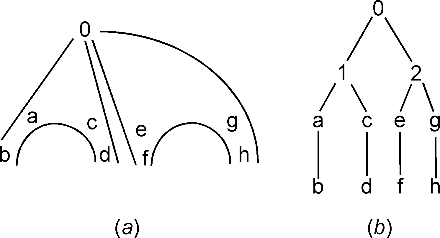
Figure 10. (a) shows $S_{8}$ and (b) shows $T_{8}$ of Example 3.4(c). See also Remark 3.16.

Definitions 3.5 (Directions in O-trees). In a rooted tree $T$, each node that is not a leaf has sons $u_{1},...,u_{p},...$ from which are issued subtrees whose sets of nodes are the sets $N_{\leq}(u_{i})$. In O-trees directions replace such subtrees that need not exist in O-trees because a node may have no son (for example node 2 of the tree $T_{3}$ of Figure 9(a)).

1. Let $T=(N,\leq)$ be an O-tree. Let $L\subseteq N$ be linearly ordered and upwards closed. It is a line according to Definition 1.1. Two nodes $x$ and $y$ in $N_{<}(L):=\{w\in N\mid w<L\}$ are in the same direction w.r.t. $L$ if $x\leq u$ and $y\leq u$ for some $u\in N_{<}(L)$. This is an equivalence relation that we denote by $\sim_{L}$. Clearly, $x\leq y$ implies $x\sim_{L}y$. Each equivalence class is called a direction relative to $L$. We denote by $Dir_{L}(x)$ the direction relative to $L$ that contains $x$ such that $x<L$. The O-tree is binary if each such line $L$ has at most two directions.

2. Let $S=(N,B)$ satisfy Axioms A1-A6 (but not necessarily A8) and $r$ be any node taken as root. Then $T(S,r).:=(N,\leq_{r})$ is an O-tree. If $x$ and $y$ in $N$ are incomparable, the set $L_{>}(x,y)$ is an upwards closed line that contains $r$, but not $x$ and $y$. We denote by $\mathfrak{L}$ the countable set of such lines ($\mathfrak{L}$ $\subset\mathcal{K}$ defined in Definition 1.3).

3. For $L=L_{>}(x,y)\in\mathfrak{L}$, we denote by $\mathfrak{D}(L)$ the set of directions relative to $L$. There are at least two different ones, $Dir_{L}(x)$ and $Dir_{L}(x)$ . We have $L=L_{>}(N_{<}(L))$ and $N_{<}(L)$ is the disjoint union of the directions in $\mathfrak{D}(L).$

Examples 3.6.

1. In the O-tree $T_{3}$ of Figure 9(a) (defined for proving Proposition 2.15(3)), $L_{>}(b,c)$ is the set $\mathbb{Q}_{>}(\sqrt{2})$ of rational numbers larger that $\sqrt{2}$ and the associated three directions are $\{a,b\}$,$\{c,d\}$ and $\mathbb{Q}_{<}(\sqrt{2}):=\mathbb{Q}-\mathbb{Q}_{>}(\sqrt{2})$.

2. We consider again the join-tree $T:=(Seq_{+}(\mathbb{Q}),\preceq)$ of Example 1.2(4) defined by Fraïssé. The partial ordered $\preceq$ is defined as follows :

   $\qquad(x_{1},...,x_{n})\preceq(y_{1},...,y_{m})$ if and only if

   $\qquad n\geq m$, $(x_{1},...,x_{m-1})=(y_{1},...,y_{m-1})$ and $x_{m}\leq y_{m}$.

   The join of two incomparable nodes $\boldsymbol{x}:=(x_{1},...,x_{n})$ and $\boldsymbol{y}:=(y_{1},...,y_{m})$ is $\boldsymbol{z}=(z_{1},...,z_{p})$ if we have $p\leq n$, $\boldsymbol{x}=(z_{1},...,z_{p-1},x_{p},...,x_{n}),z_{p}>x_{p}$ and $\boldsymbol{y}=(z_{1},...,z_{p-1},z_{p},$ $y_{p+1},...,y_{m})$. Then, the directions relative to $L=L_{>}(\boldsymbol{x},\boldsymbol{y})=L_{>}(\boldsymbol{z})$ are :

   $Dir_{L}(\boldsymbol{x})=\{(z_{1},...,z_{p-1},u_{p},u_{p+1},...,u_{q})\mid u_{p},...,u_{q}\in\mathbb{Q},u_{p}\leq z_{p}\}$ and

   $Dir_{L}(\boldsymbol{y})=\{(z_{1},...,z_{p},u_{p+1},...,u_{q})\mid u_{p+1},...,u_{q}\in\mathbb{Q}\}$.

   This join-tree is binary.

Lemma 3.7. Let $S=(N,B),r$ and $<_{r}$ be as in Lemma 3.2, and $L\in\mathfrak{L}$. Let $u,v\in D$ for some direction $D$ in $\mathfrak{D}(L)$ (see Definition 3.5). Let $m\in L$ and $w\in N$. Then $B(u,m,w)$ if and only if $B(v,m,w)$.

Proof.

We will denote $\leq_{r}$ by $\leq$. Related notations are $<$, $\sqcup$ and $\bot.$

We have $\{u,v\}<a<m$ for some $a\in D$, hence $B(u,a,m)$ and $B(v,a,m)$ by Lemma 3.2(2). If $B(u,m,w)$ we have $B^{+}(u,a,m,w)$ by A5, hence $B(a,m,w)$. From this fact and $B(v,a,m),$ we get $B^{+}(v,a,m,w)$ by A4, hence $B(v,m,w)$. $\square$

It follows that we can define, for $D,D^{\prime}\in\mathfrak{D}(L)$ and $m\in L$:

$B(D,m,D^{\prime}):\Longleftrightarrow B(u,m,w)$ for some $u\in D$ and $w\in D^{\prime}.$

By Lemma 3.7, we have (directions are not empty by definition) :

$B(D,m,D^{\prime})\Longleftrightarrow B(u,m,w)$ for all $u\in D$ and $w\in D^{\prime}.$

In particular, we do not have $B(D,m,D).$ ∎

Lemma 3.8. Let $S=(N,B)$ satisfy A1-A6 and A8. Let $r\in N$, $T(S,r):=(N,\leq_{r})$ and $m\in L\in\mathfrak{L}$. The binary relation $\lnot B(D,m,D^{\prime})$ for $D,D^{\prime}\in\mathfrak{D}(L)$ is an equivalence relation.

Proof.

Reflexivity and symmetry are clear. Assume that we have $\lnot B(D,m,$ $D^{\prime})$ and $\lnot B(D^{\prime},m,D^{\prime\prime})$ for distinct directions $D,D^{\prime},D^{\prime\prime}$. Hence, by Lemma 3.7, we have $\lnot B(u,m,v)$ and $\lnot B(v,m,w)$ for some $u,v,w$ respectively in $D,D^{\prime},D^{\prime\prime}$. For a contradiction, we assume that $B(u,m,w)$ holds.

We have $\lnot B(u,m,v)$ as observed above. If $B(m,u,v)$ we have $m<u$ or $v<u$ by Lemma 3.3(2), but we know that $u<m$ and $u\bot v.$ Hence, we have $\lnot B(m,u,v)$ and similarly, $\lnot B(m,v,u)$. We have $\lnot A(m,u,v)\wedge B(w,m,u)$, and A8 gives $B(w,m,v)$, contradicting an assumption.

Hence, $\lnot B(u,m,w)$ holds for all $u,w$ respectively in $D,D^{\prime\prime}$ and we have $\lnot B(D,m,D^{\prime\prime})$. ∎

Definition 3.9 (Independent directions). Let $S=(N,B)$ satisfy A1-A6 and A8, $r\in N$, and $m\in L\in\mathfrak{L}$, relative to $T(S,r):=(N,\leq_{r}).$

1. If $D$, $D^{\prime}\in\mathfrak{D}(L)$, we define $D\approx_{L}D^{\prime}$ if $B(D,m,D^{\prime})$ holds for no $m\in L$. By Lemma 3.2(2), $B(D,m,D^{\prime})$ can hold only if $m$ is the smallest element of $L$. Hence, $D\approx_{L}D^{\prime}$ holds if and only if, either $L$ has no smallest element or $B(D,\min(L),D^{\prime})$ does not hold. Hence, by Lemma 3.8, $\approx_{L}$ is an equivalence relation. We say that $D$ and $D^{\prime}$  are independent if $D\approx_{L}D^{\prime}$ because they are not ”linked” through any $m\in L$ such that $B(D,m,D^{\prime})$ holds.

2. For each $D\in\mathfrak{D}(L)$, we denote by $D_{\approx}$ the union of the directions that are $\approx_{L}$-equivalent to $D$. The sets $D_{\approx}$ form a partition of $N_{<}(L)$. We define $\mathcal{C}:=\mathcal{C}_{1}\uplus\mathcal{C}_{2}$ as the set of downward closed subsets of $N$ such that:

   $\mathcal{C}_{1}:=\{N_{\leq}(x)\mid x\in N\}$ (in particular $N=N_{\leq}(r)$) and

   $\mathcal{C}_{2}:=\{D_{\approx}\mid D\in\mathfrak{D}(L)$, $L\in\mathfrak{L}$ and $D_{\approx}$ is the union of at least two directions}.

We pause with technicalities for explaining how we will use these definitions and lemmas.

Consider the structure $S_{8}=(N_{8},B_{8})$ of Figure 10(a), used in Example 3.4(c). The rooted tree $T(S_{8},0)$ is $T_{8}$ shown in Figure 10(b) minus the nodes 1 and 2. There are in $T(S_{8},0)$ four directions relative to $L:=\{0\}=L_{>}(a,c)=L_{>}(a,e)=L_{>}(g,c)$. They are $D(a)=\{a,b\}$, the direction of $a$, and similarly, $D(c)=\{c,d\},D(e)=\{e,f\}$ and $D(g)=\{g,h\}$.

Let $B:=B_{8}$. We have $B(D(a),0,D(e))$, $B(D(c),0,D(e))$, $B(D(a),0,D(g))$ and $B(D(c),0,D(g))$ because $B$ contains the triples $(a,0,e),$ $(c,0,e),(a,0,g)$ and $(c,0,g)$ (by clauses (ii) in Example 3.4(c)). But we have neither $B(D(a),0,D(c))$ nor $B(D(e),0,D(g)).$ The two equivalences in $\mathfrak{D}(L)$ are $D(a)\approx_{L}D(c)$ and $D(e)\approx_{L}D(g).$

Since we have $B(b,a,c)$ we must have in any join-tree $R$ such that $T(S_{8},0)\subseteq R$ and $B=B_{R}[N_{8}]$ an element $x$ such that in $B_{R}^{+}(b,a,x,c)$ holds with $b<_{R}a<_{R}x<_{R}0$ and $c<_{R}x<_{R}0$. To build such a tree, we must add $x$, and similarly $y$ such that $f<_{R}e<_{R}y<_{R}0$ and $g<_{R}y<_{R}0$. They are the nodes 1 and 2 in Figure 10(b), formally defined as the two sets $D(a)\uplus D(c)=\{a,b,c,d\}$ and $D(e)\uplus D(g)=\{e,f,g,h\}$ that form $\mathcal{C}_{2}$.

In the general construction, for each $\approx_{L}$-equivalence class $E$ of independent directions, we introduce in $T(S,r)$ an element $x$ such that, for each direction $D$ in $E$, we have $D<x<L$. Such an element is added only for an equivalence class $E$ containing at least two different equivalent directions. It is formally defined as the union of the directions in $E$. These added elements correspond bijectively to the sets in $\mathcal{C}_{2}$.

Lemma 3.10. Let $S=(N,B)$ and $r\in N$ be as in Lemma 3.8, from which we get $\mathcal{C}$ by Definition 3.9(b).

(1) The family $\mathcal{C}$ is not overlapping.

(2) It is first-order definable in $S$.

Proof.

1. Consider $E$ and $E^{\prime}$ in $\mathcal{C}$ such that $w\in E\cap E^{\prime}$.

   There are three possible cases to consider.

   Case 1 : $E=N_{\leq}(x),E^{\prime}=N_{\leq}(y)$. Then $x\leq y$ or $y\leq x$ because $w\leq x$ and $w\leq y$, which gives $E\subseteq E^{\prime}$ or $E^{\prime}\subseteq E$.

   Case 2 : $E=N_{\leq}(x),w\leq x,E^{\prime}=D_{\approx}$, $D=Dir_{L}(w)$ where $L\in\mathfrak{L}$. Then $x<L$ (in particular if $x=w)$ or $x\in L$, which gives $E\subseteq D\subseteq E^{\prime}$ or $E^{\prime}\subseteq E.$

   Case 3$\ :E=D_{\approx}$, $D\in\mathfrak{D}(L)$, and $E^{\prime}=D_{\approx}^{\prime},D^{\prime}\in\mathfrak{D}(L^{\prime})$. Then $L\cup L^{\prime}\subseteq L_{>}(w)$, hence $L^{\prime}\subset L$ or $L\subset L^{\prime}$ or $L=L^{\prime}$ . In the first case, we have $Dir_{L}(w)\subseteq E\subseteq N_{\leq}(x)$ for any $x\in L-L^{\prime}$. We have $x<L^{\prime}$. Then, $N_{\leq}(x)\subseteq Dir_{L^{\prime}}(w)\subseteq E^{\prime}$.  The second case is similar and the last one gives $Dir_{L}(w)=Dir_{L^{\prime}}(w)$, hence, $E=E^{\prime}.$

   
   

2. The set $\mathcal{C}$ is relative to a rooted O-tree $T(S,r)$ where $r\in N$. We will construct an FO formula $\varphi(X,r)$ (not depending on $S$) such that for every $r$ and $X\subseteq N$,

   $S=(N,B)\models\varphi(X,r)$  if and only if $X\in\mathcal{C}$.

   Since $\mathcal{C}$ is defined from $T(S,r)$, this formula will have the free variable $r$. The partial order $\leq_{r}$ (denoted by $\leq$) is FO definable in $S$ in terms of $r$, and so is incomparability, denoted by $\bot$.

   An FO formula $\varphi_{1}(X,r)$ can express that $X=N_{\leq}(x)$ for some $x\in N$.

   Next we define $\varphi_{2}(X,r)$ intended to characterize the sets $D_{\approx}$. Let $x$ and $y$ be incomparable in $T(S,r)=(N,\leq).$ Let $L=L_{>}(x,y)$ and $u,v<L.$ The nodes $u$ and $v$ are in the direction $Dir_{L}(u)\in\mathfrak{D}(L)$ if and only if :

   $(N,B)\models\exists w[u<w\wedge v<w\wedge\forall z(z\in L\Longrightarrow w<z)],\$

   which can be expressed by an FO formula $\alpha(r,x,y,u,v)$ because $z\in L$ is FO expressible in terms of $r,x$ and $y$. Similarly, $u$ and $v$ are in a same set $D_{\approx}$ for some set $D\in\mathfrak{D}(L)$ (then $D_{\approx}=Dir_{L}(u)_{\approx}$) if and only if :

   $(N,B)\models\forall z[z\in L\Longrightarrow\lnot B(u,z,v)],\$

   which can be expressed by an FO formula $\sigma(r,x,y,u,v)$.

   If $u<L$, the set $Dir_{L}(u)_{\approx}$ is the union of at least two directions in $\mathfrak{D}(L)$ if and only if :

   $(N,B)\models u<L\wedge\exists v[v<L\wedge\sigma(r,x,y,u,v)\wedge\lnot\alpha(r,x,y,u,v)]$

   which is expressed by an FO formula $\delta(r,x,y,u)$ (for convenience, this formula includes the condition $u<L$).

   We let finally $\varphi_{2}(X,r)$ be the FO formula that :

   $\exists x,y[x\bot y\wedge\exists u(u\in X\wedge\delta(r,x,y,u))\wedge\forall u(u\in X\Longrightarrow\forall v[v\in X\Longleftrightarrow\sigma(r,x,y,u,v)])].$

   It expresses that $X=$ $Dir_{L_{>}(x,y)}(u)_{\approx}$ for some incomparable elements $x,y$, and that $X$ is the union of at least two directions in $\mathfrak{D}(L_{>}(x,y))$.

   Hence, the formula $\varphi_{1}(X,r)\vee\varphi_{2}(X,r)$ expresses that $X\in\mathcal{C}$. ∎

We will use $\mathcal{C}$ to build a join-tree witnessing that $S$ is in IBQT. With the notation of Lemma 3.10, we have the following obvious facts.

Lemma 3.11. For all $x,y\in N$, $D\in\mathfrak{D}(L)$, $D^{\prime}\in\mathfrak{D}(L^{\prime})$ and $L,L^{\prime}\in\mathfrak{L}$ we have:

1. $N_{\leq}(x)\subset N_{\leq}(y)$ if and only if $x<y$.

2. $N_{\leq}(x)\subset D_{\approx}\$if and only if $x<L$ and $D_{\approx}=Dir_{L}(x)_{\approx},$

3. $D_{\approx}\subset N_{\leq}(x)$ if and only if $x\in L$,

4. $D_{\approx}\subset D_{\approx}^{\prime}$ if and only if $L^{\prime}\subset L$; if $\ D_{\approx}\subset D_{\approx}^{\prime}$, we have$\ D_{\approx}\subseteq N_{\leq}(x)\subseteq D_{\approx}^{\prime}$ for every $x$ in $L-L^{\prime}.$

In the next three lemmas, $S$ and the related objects are as in Lemma 3.10.

Lemma 3.12. The structure $T(\mathcal{C}):=(\mathcal{C},\subseteq)$ is a join-tree.

Proof.

First, $T(\mathcal{C}):=(\mathcal{C},\subseteq)$ is an O-tree because if $E\subseteq E^{\prime}$ and $E\subseteq E^{\prime\prime}$, we have $E^{\prime}\subseteq E^{\prime\prime}$ or $E^{\prime\prime}\subseteq E^{\prime}$ by Lemma 3.10(1). Next we consider $E$ and $E^{\prime}$, incomparable in $T(\mathcal{C})$. They are disjoint. We will prove that they have a join $E\sqcup_{T(\mathcal{C})}E^{\prime}$ in $T(\mathcal{C}).$ There are three cases and several subcases.

Case 1 : $E=N_{\leq}(x),E^{\prime}=N_{\leq}(y)$ where $x\bot y$ .

Subcase 1.1 : $(x,m,y)\notin B$ for every $m$ in $L:=L_{>}(x,y)$. Then $Dir_{L}(x)\approx_{L}Dir_{L}(y)$ and $E^{\prime\prime}:=Dir_{L}(x)_{\approx}\supseteq E\uplus E^{\prime}$. We have $Dir_{L}(x)_{\approx}\in\mathcal{C}$ because $Dir_{L}(x)\neq Dir_{L}(y)$.

We prove that $E^{\prime\prime}=E\sqcup_{T(\mathcal{C})}E^{\prime}.$ If this is not the case, we could have $E^{\prime\prime}\supset N_{\leq}(z)\supseteq E\uplus E^{\prime}$. But then $x,y<z$ by Lemma 3.11(1), hence $z\in L$ and $N_{\leq}(z)\supseteq N_{<}(L).$ So we cannot have $N_{\leq}(z)\subset E^{\prime\prime}\subseteq N_{<}(L).$

Otherwise, we have $E^{\prime\prime}\supset D_{\approx}^{\prime}\supseteq E\uplus E^{\prime}$. By Lemma 3.11(2), we have $D_{\approx}^{\prime}=Dir_{L^{\prime}}(x)_{\approx}=Dir_{L^{\prime}}(y)_{\approx}$ and $L\subset L^{\prime}$. Let $z\in L^{\prime}-L$. Then $x,y<z$, hence $z\in L$, contradicting the choice of $z$. Hence, $Dir_{L}(x)_{\approx}=E\sqcup_{T(\mathcal{C})}E^{\prime}.$

Note that $E^{\prime\prime}$ is not of the form $N_{\leq}(z)$ for any $z$ because it is the disjoint union of at least two directions in $\mathcal{D}(L)$. If $E^{\prime\prime}=N_{\leq}(z)$, then $z$ would belong to one direction, say $F$, and all these directions, in particular $Dir_{L}(x)$ and $Dir_{L}(y),$ would be included in $F,$ hence equal to $F$ because directions in $\mathcal{D}(L)$ do not overlap.

Subcase 1.2 : $(x,m,y)\in B$ where $m=x\sqcup_{T}y=\min(L)$. Let $E^{\prime\prime}:=N_{\leq}(m)\supset E\uplus E^{\prime}$.

We claim that $E^{\prime\prime}=E\sqcup_{T(\mathcal{C})}E^{\prime}.$ If this is not the case, we could have $E^{\prime\prime}=N_{\leq}(m)\supset N_{\leq}(z)\supseteq E\uplus E^{\prime}$. But then $\{x,y\}<z<m$, hence $m$ is not the join of $x$ and $y$. Otherwise, $E^{\prime\prime}=N_{\leq}(m)\supset D_{\approx}^{\prime}\supseteq E\uplus E^{\prime}$ where $D_{\approx}^{\prime}=Dir_{L^{\prime}}(x)_{\approx}=Dir_{L^{\prime}}(y)_{\approx}$ and $L\subset L^{\prime}$. Let $z\in L^{\prime}-L$. Then $\{x,y\}<z<m$, hence $m$ is not the join of $x$ and $y$. Hence, $N_{\leq}(m)=E\sqcup_{T(\mathcal{C})}E^{\prime}.$

Case 2 : $E=N_{\leq}(x),E^{\prime}=Dir_{L}(y)_{\approx}$. Since $N_{\leq}(x)\cap Dir_{L}(y)_{\approx}=\emptyset$, we do not have $Dir_{L}(y)\approx_{L}Dir_{L}(y)$, hence we have $(x,m,y)\in B$ for some $m$ that must be $x\sqcup_{T(S,r)}y=\min(L).$ We have $N_{\leq}(m)=E\sqcup_{T(\mathcal{C})}E^{\prime}$ as in Subcase 1.2.

Case 3$\ :E=D_{\approx}$, $D\in\mathfrak{D}(L)$, and $E^{\prime}=D_{\approx}^{\prime},D^{\prime}\in\mathfrak{D}(L^{\prime})$. If $L=L^{\prime}$ then, as $D_{\approx}\neq D_{\approx}^{\prime}$, we have $B(D,m,D^{\prime})$ where $m=\min(L)$, and then $E\sqcup_{T(\mathcal{C})}E^{\prime}=N_{\leq}(m)$, as in Case 2.

Otherwise, $L$ and $L^{\prime}$ are incomparable by Lemma 3.11(4) since $E$ and $E^{\prime}$ are so, and $r\in L\cap L^{\prime}$. Hence, there are $w\in L-L^{\prime}$  and $w^{\prime}\in L^{\prime}-L$. We have $L\cap L^{\prime}=L_{>}(w,w^{\prime})$. If $(w,m,w^{\prime})\in B$ for some $m\in L\cap L^{\prime}$ then $m=\min(L_{>}(w,w^{\prime}))$ and $N_{\leq}(m)=E\sqcup_{T(\mathcal{C})}E^{\prime}$ as in Case 2.

If $(w,m,w^{\prime})\in B$ for no $m\in L\cap L^{\prime}$ then, $F\approx_{L\cap L^{\prime}}F^{\prime}$ where $F=Dir_{L\cap L^{\prime}}(w)$ and $F^{\prime}=Dir_{L\cap L^{\prime}}(w^{\prime})$. We claim that $F_{\approx}$ is $E\sqcup_{T(\mathcal{C})}E^{\prime}$ as in Subcase 1.1. ∎

The next two lemmas prove that the join-tree $T(\mathcal{C})$ witnesses that $S$ is in IBQT. We identify $N$ with the subset $\mathcal{C})_{1}$ of $N_{T(\mathcal{C})}$.

Lemma 3.13. $B\subseteq B_{T(\mathcal{C})}[N]$.

Proof.

We recall that $<$ denotes $<_{r}=<_{T(S,r)}$ which is, by Fact (1) of Lemma 3.11, the restriction of $<_{T(\mathcal{C})}$ to $N$. The joins in $T(S,r)$ and $T(\mathcal{C})$ are not always the same.

Consider $(x,y,z)\in B$. By Lemma 3.3(2), we have $x<y$ or $z<y$. Assume $x<y$. If $y<z$ then $x<_{T(\mathcal{C})}y<_{T(\mathcal{C})}z$, hence $(x,y,z)\in B_{T(\mathcal{C})}[N]$. If $z<y$, then $y=x\sqcup_{T(S,r)}z$, by Lemma 3.2(3). We are in Subcase 1.2 of Lemma 3.12, hence, $y=x\sqcup_{T(\mathcal{C})}z$ and $(x,y,z)\in B_{T(\mathcal{C})}$. The last case is $y\bot z.$ Let $E:=y\sqcup_{T(\mathcal{C})}z$. We have $x<y<_{T(\mathcal{C})}E$, hence $(x,y,E)\in B_{T(\mathcal{C})}$, and also $(y,E,z)\in B_{T(\mathcal{C})}$, hence $(x,y,z)\in B_{T(\mathcal{C})}$.

The case $z<y$ is similar. ∎

Lemma 3.14. $B_{T(\mathcal{C})}[N]\subseteq B$.

Proof.

Let $x,y,z\in N$ be such that $(x,y,z)\in B_{T(\mathcal{C})}.$

If $x<_{T(\mathcal{C})}y<_{T(\mathcal{C})}z$, or $z<_{T(\mathcal{C})}y<_{T(\mathcal{C})}x$, then $x<y<z$, or $z<y<x$ since $<$ is the restriction of $<_{T(\mathcal{C})}$ to $N$. Hence, $(x,y,z)\in B$ by the definition of $<$ as $<_{T(S,r)}.$

Otherwise $x<y\leq_{T(\mathcal{C})}E>_{T(\mathcal{C})}z$ or $x<_{T(\mathcal{C})}E\geq_{T(\mathcal{C})}y>z$, where $x$ and $z$ are incomparable in $T(\mathcal{C}),$ hence also in $T(S,r),$ and $E=x\sqcup_{T(\mathcal{C})}z$. We assume the first.

Case 1 : $y\bot z$ in $T(S,r)$. Then we have $(x,y,z)\in B$ by Lemma 3.3(1) since $x<y$.

Case 2 : If $y$ and $z$ are comparable, the case $y<z$ has been first considered. Otherwise, $y>z$, hence $y\geq_{T(\mathcal{C})}E=x\sqcup_{T(\mathcal{C})}z$. As $y\leq_{T(\mathcal{C})}E,$ we must have $y=E$. Hence we are in Subcase 1.2 of Lemma 3.12, with $y=x\sqcup_{T(S,r)}z$ so that $(x,y,z)\in B$. ∎

Proof of Theorem 3.1.

From $(N,B)$ satisfying A1-A6 and A8, we have built a join-tree $T(\mathcal{C})$ whose nodes $\mathcal{C}$ contains $N$ (with $x\in N$ identified with $N_{\leq}(x)\in N_{T(\mathcal{C})}$) such that, by Lemmas 3.13 and 3.14, the restriction of its betweenness relation $B_{T(\mathcal{C})}$ to $N$ is $B$. Hence, together with Theorem 2.9, a structure $(N,B)$ is in IBQT if and only if it satisfies A1-A6 and A8. ∎

We know from Definition 10 and Proposition 17 of [6]  that a quasi-tree $(N,B)$ is the betweenness relation of a tree if and only if $B$ is discrete, i.e., that each set $[x,y]_{B}:=\{x,y\}\cup\{z\in N\mid B(x,z,y)\}$ is finite (cf. Definition 2.8(a)).

Corollary 3.15. A structure $S=(N,B)$ is an induced betweenness relation in a tree if and only if it satisfies axioms A1-A6, A8 and is discrete. These conditions are monadic second-order expressible.

Proof.

An induced substructure $S=(N,B)$ of a discrete one is discrete, which gives the ”only if” directions by Theorem 2.9. Conversely, if $S=(N,B)$ satisfies axioms A1-A6, A8 and is discrete, then for all $x,y\in N$ such that $x\leq_{T(S,r)}y,$ the set $\{z\in N\mid x\leq_{T(S,r)}z\leq_{T(S,r)}y\}=[x,y]_{B}$ is finite. Hence, $T(S,r)$ is a rooted tree.

For all $x,y\in N_{T(\mathcal{C})}$ such that $x\leq_{T(\mathcal{C})}y,$ the set $\{z\in N_{T(\mathcal{C})}\mid x\leq_{T(\mathcal{C})}z\leq_{T(\mathcal{C})}y\}$ is finite because, by Lemma 3.11(4), its number of elements belonging to $\mathcal{C}_{2}$ is at most one plus its number of elements belonging to $\mathcal{C}_{1}$, that is finite as observed above. Hence, $T(\mathcal{C})$ is a rooted tree.

Recall from Section 1.4 that the finiteness of a linear order is MSO expressible. On each set $[x,y]_{B}$ such that $x<_{T(S,r)}y,$ the linear order $\leq_{T(S,r)}$ is FO definable. Hence, the finiteness of $[x,y]_{B}$ is MSO expressible. ∎

Examples and Remarks 3.16. [About the proof of Theorem 3.1.]

1. Consider the structure $S_{8}$ of Figure 10(a). The O-tree $T(S_{8},0)$ is $T_{8}$ (in Figure 10(b)) minus the nodes 1 and 2. As observed above, there are four directions relative to $L:=\{0\}=L_{>}(a,c)$ : $D(a)$, the direction of $a$, and similarly, $D(c),D(e)$ and $D(g)$. The two sets of $\mathcal{C}_{2}$ are $D(a)_{\approx}=D(a)\uplus D(c)=\{a,b,c,d\}$ and $D(e)_{\approx}=D(e)\uplus D(g)=\{e,f,g,h\}.$ The nodes 1 and 2 of Figure 10(b) represent the two nodes $D(a)_{\approx}$ and $D(e)_{\approx}$ added to $T(S_{8},0)$ to form the tree $T_{8}$ such that $S_{8}=B_{T_{8}}[\{0,a,...,h\}].$

2. Consider the O-tree of Figure 8 and its betweenness relation to which we add the fact $B(a,b,c)$ (and of course $B(c,b,a)).$ Let $L:=\mathbb{N}$. This new structure satisfies A1-A6 and A8. The two directions relative to $L$ are $\{a,b\}$ and $\{c\}$. They are $\approx_{L}$-equivalent. Only one node is added : $\{a,b,c\}=D(a)\uplus D(c)$.

3. Let $T=(N,\leq)$ be a join-tree with root $r$. Let $S:=(N,B_{T})$. Then, $T=T(S,r)$. Let us apply the construction of Theorem 3.1.    Each$\ L\in\mathfrak{L}$ has a minimal element because $T$ is a join-tree. By Definition 3.9(a), no two different directions relative to $L$ are $\approx_{L}$-equivalent. Hence, The family $\mathcal{C}$ consists only of the sets $N_{\leq}(x)$ and so, $T(\mathcal{C})=T(S,r)=T$.

4. If $S=(N,B)$ is an induced betweenness in a quasi-tree, then any node $r$ can be taken as root for defining an O-tree $T(S,r)$ and from it, a join-tree $T(\mathcal{C})$. This fact generalizes the observation that the betweenness in a tree $T$ does not dependent on any root. Informally, quasi-trees and induced betweenness in quasi-trees are ”undirected notions”. This will not be true for betweenness in O-trees. See the remark about $U$ in the proof of Proposition 2.15, Part (2).

5. If $S=(N,\emptyset)$, then $T(S,r)$ consists of the root $r$ having sons $u$ for all $u\in N-\{r\}$. These sons are in pairwise independent directions relative to $\{r\}$. The rooted tree $T(\mathcal{C})$ is $T(S,r)$ augmented with a unique new node $x$ corresponding to $N-\{r\}=D_{\approx}$ where $D$ is $\{u\}$ for any $u\in N-\{r\}$. We have $u<_{T(\mathcal{C})}x<_{T(\mathcal{C})}r$ for each $u\in N-\{r\}$.

3.1.2. Betweenness in rooted O-trees

We let BO_root be the class of betweenness relations of rooted O-trees. These relations satisfy A1-A6.

Proposition 3.17. The class BO_root is axiomatized by a first-order sentence.

Proof.

Consider $S=(N,B)$. If $B$ is the betweenness relation of an O-tree $(N,\leq)$ with root $r$, then, $\leq$ is nothing but $\leq_{r}$ defined before Lemma 3.2 from $B$ and $r$. Let $\varphi$ be the FO sentence that expresses properties A1-A6 (relative to $B$) together with the following one:

A9 : there exists $r\in N$ such that the O-tree $T(S,r):=(N,\leq_{r})$ whose partial order is defined by $x\leq_{r}y:\Longleftrightarrow x=y\vee y=r\vee B(x,y,r)$ has a betweenness relation $B_{T(S,r)}$ equal to $B$.

That $S$ satisfies A1-A6 insures that $(N,\leq_{r})$ is an O-tree with root $r$. The sentence $\varphi$ holds if and only if $S$ is in BO_root. When it holds, the found node $r$ defines via $\leq_{r}$ the relevant O-tree. ∎

The following counter-example shows that we do not obtain an FO axiomatization of the class BO.

Example 3.18 (BO_root is properly included in BO). Let $T$ be the O-tree with set of nodes $\mathbb{Q}$ and defining partial order $\preceq$ such that $x\preceq y:\Longleftrightarrow x\leq y\wedge y\in\mathbb{Q}-\mathbb{Z}$ (see Figure 11). Any two elements of $\mathbb{Z}$ are incomparable and no two incomparable elements have a join. We claim that $B_{T}$ is not in BO_root. We have $B_{T}=\{(i,j,k),(k,j,i)\mid i,j,k\in\mathbb{Q},j,k\notin\mathbb{Z}$ and $i<j<k\}$.

Assume that $B_{T}\ =B_{U}$ for some O-tree $U$ with root $r\in\mathbb{Q}$. We will derive a contradiction.

If $r\in\mathbb{Z}$ we take, without loss of generality, $r=0$. Let $a=-1/2$ and $b=-3/2$. These two nodes are incomparable in $U$ otherwise, we would have $(0,a,b)$ or $(0,b,a)$ in $B_{U}=B_{T}$ which is false. Hence $(a,0,b)\in B_{U}$, but $(a,0,b)\notin B_{T}.$

If $r\in\mathbb{Q}-\mathbb{Z}$ we take, without loss of generality, $r=1/2$. Let $a=1$ and $b=2$. These two nodes are incomparable in $U$ otherwise, we would have $(1/2,a,b)$ or $(1/2,b,a)$ in $B_{U}=B_{T}$ which is false. Hence $(a,1/2,b)\in B_{U}$, but $(a,1/2,b)\notin B_{T}.$

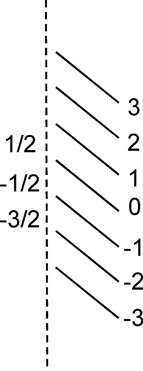
Figure 11. The O-tree of Example 3.18.

3.2. Monadic second-order axiomatizations

3.2.1. Betweenness in O-trees.

We will prove that the class BO is axiomatized by a monadic second-order sentence. In the proof of Proposition 3.17, we have defined from $S=(N,B)$ satisfying A1-A6 and $r\in N$ a candidate partial order $\leq_{r}$ for $(N,\leq_{r})$ to be an O-tree with root $r$ whose betweenness relation would be $B$. The order $\leq_{r}$ being expressible by a first-order sentence, we finally obtained a first-order characterization of BO_root. For BO, a candidate order will be defined from a line, not from a single node. It follows that we will need for our construction a set quantification.

The next lemma is Proposition 5.3 of [7].

Lemma 3.19. Let $(L,B)$ satisfy properties A1-A7’. Let $a,b$ be distinct elements of $L$. There exist a unique linear order $\leq$ on $L$ such that $a<b$ and $B_{(L,\leq)}=B$. This order is quantifier-free definable, in terms of $a$ and $b,$ in the relational structure $(L,B)$.

We will denote this order by $\leq_{L,B,a,b}$. There is a quantifier-free formula $\lambda,$ written with the ternary relation symbol $B,$ such that, for all $a,b,u,v$ in $L$, $(L,B)\models\lambda(a,b,u,v)$ if and only if $u\leq_{L,B,a,b}v$. We recall from Definition 1.1(b) that a line $L$ in an O-tree $T$ is a linearly ordered set that is convex, i.e., $y\in L$ if $x,z\in L$ and $x\leq_{T}y\leq_{T}z$.

Lemma 3.20. Let $T=(N,\leq_{T})$ be an O-tree and $L$ a maximal line in $T$ that has no largest node. Let $a,b\in L$, such that $a<_{L}b$, where $<_{L}$ is the restriction of $<_{T}$ to $L$.

1. The partial order $\leq_{T}$ is first-order definable in a unique way in the structure ($N,B_{T})$ in terms of $L,\leq_{L},a$ and $b$.

2. It is first-order definable in ($N,B_{T})$ in terms of $L,a$ and $b$.$\square$

Proof.

The line $L$ is upwards closed and infinite.

Let $x,y\in N$. We first prove the following facts.

Fact 1 : If $x,y\in L$, then $x<_{T}y$ if and only if $x<_{L}y.$

Fact 2 : If $x\notin L,y\in L,$ then $x<_{T}y$ if and only if $B_{T}(x,y,z)$ holds for some $z\in L$ such that $z>_{L}y.$

Fact 3 : If $x,y\notin L,$ then $x<_{T}y$ if and only if $B_{T}^{+}(x,y,z,u)$ holds for some $z,u$ in $L$, such that $u>_{L}z.$

Fact 1 is clear from the definitions.

For Fact 2, we have some $z>_{L}y$ because $L$ has no largest element. If $x<_{T}y<_{L}z$, then $B_{T}(x,y,z)$ holds.

Assume now that $B_{T}(x,y,z)$ holds for some $z>_{L}y.$ By the definition of $B_{T}$, we have $x<_{T}y\leq_{T}x\sqcup_{T}z$ or $z<_{T}y\leq_{T}x\sqcup_{T}z$. Since $z>_{L}y,$ we cannot have $z<_{T}y.$ Hence, $x<_{T}y.$  (We have actually $B_{T}(x,y,z)$ for every $z>_{L}y).$

For Fact 3, we note that for every $y\notin L$, we have some $z\in L$, $z>_{T}y$ : take for $z$ any upper-bound of $y$ and some element of $L$, then  $z\in L$ because $T$ is an O-tree. Hence, we have $z,u\in L$ such that $y<_{T}z<_{L}u$ because $L$ has no largest element, hence $B_{T}(y,z,u)$ holds by Fact 2.

If $x<_{T}y$, we have $x<_{T}y<_{T}z$ hence $B_{T}^{+}\ (x,y,z,u)$ hold (by A4) since we have $B_{T}(x,y,z)$ and $B_{T}(y,z,u).$

Assume now for the converse that $B_{T}^{+}(x,y,z,u)$ holds for $z,u\in L$ such that $z<_{L}u$. We have $B_{T}(x,y,z)$ and $z>_{T}y$ by Fact 2 (since we have $B_{T}(y,z,u)$). By the definition of $B_{T}$, we have $x<_{T}y\leq x\sqcup_{T}z$   or $\ z<_{T}y\leq x\sqcup_{T}z$. Since $z>_{T}y,$ we cannot have $z<_{T}y$, hence, $x<_{T}y.$

We now prove the two assertions of the statement.

(1) The above four facts show that $\leq_{T}$ is first-order definable in $(N,B_{T})$ in terms of $L,\leq_{L},a$ and $b$.  More precisely, Facts 1,2 and 3 can be expressed as a first-order formula $\theta$ written with the relation symbols $L,B$ and $R$ of respective arities 1,3 and 2, such that, if $L$ is a maximal line in $T$ that has no largest node, $a,b\in L$ and $a<_{L}b$, then, for all $u,v\in N$, $(N,L,B_{T},\leq_{L})\models\theta(a,b,u,v)$ if and only if $u\leq_{T}v.$ For the validity of $\theta(a,b,u,v)$, $B_{T}$ is the value of $B,$ and $\leq_{L}$ is that of $R$.

(2) However, $\leq_{L}$ is FO definable in $(L,B_{T}[L])$ by Lemma 3.20. By replacing the atomic formulas $R(x,y)$ by $\lambda(a,b,x,y),$ we ensure that $R$ is $\leq_{L}$, hence, we obtain a first-order formula $\psi(a,b,u,v),$ written with $L$ and $B$ such that, for $u,v\in N$   we have $(N,B_{T})\models\psi(a,b,u,v)$ if and only if $u<_{T}v$ where $B_{T}$ is the value of $B$. ∎

A line in a structure $S=(N,B)$ that satisfies A1-A6 is a set $L\subseteq N$ of at least 3 elements in which any 3 different elements are aligned (cf. Section 2.1) and that is convex, i.e., is such that $[x,y]_{B}$ $\subseteq L$ for all $x,y$ in $L$.

Theorem 3.21. The class BO is axiomatized by a monadic second-order sentence.

Proof.

Let $\varphi(L)$ be the monadic second-order formula expressing the following properties of a structure $S=(N,B)$ and a set $L\subseteq N$:

1. $S$ satisfies A1-A6,

2. $L$ is a maximal line in $S$,

3. there are $a,b\in L$ such that the formula $\psi(a,b,u,v)$ of Lemma 3.20 defines a partial order $\leq$ on $N$ such that $a<b$,

4. $(N,\leq)$ is an O-tree $U$, in which $L$ is a maximal line without largest element, and

5. $B_{U}=B.$

We need a set quantification to express the maximality of $L$. All other conditions are first-order expressible.

If $S=(N,B_{T})$ is the betweenness relation of an O-tree $T=(N,\leq)$ without root, and $L$ is a maximal line in $T$, then $L$ is also a maximal line in $S$. As $T$ has no root, $L$ has no largest element. Then $\varphi(L)$ holds where $a,b\in L$ are such that $a<_{L}b$. Hence, $S\models\exists L.\varphi(L)$.

Conversely, if $S=(N,B)$ satisfies $\exists L.\varphi(L)$, then, conditions (iv) and (v) show that $S$ is in the class BO.

Together with Proposition 3.17, we can express by an MSO sentence that $(S,N)$ is the betweenness relation of an O-tree, with or without root.

A structure $S=(N,B)$ is the betweenness relation of an O-forest if and only if its connected components (cf. Remark 2.14) are the betweenness relations of O-trees. Hence, we get a monadic second-order sentence expressing that a structure $S$ is the betweenness relation of an O-forest. ∎

3.2.2. Induced betweenness in O-trees.

Next we examine in a similar way the class IBO. It is easy to see that IBO = IBO_root.

Proposition 3.22. Every structure in the class IBO  satisfies Properties A1-A6 but these properties do not characterize this class.

Proof.

Every structure $S$ in the class IBO is an induced substructure of some $S^{\prime}$ in BO, that thus satisfies Properties A1-A6. Hence, $S$ satisfies also these properties as they are expressed by universal sentences.

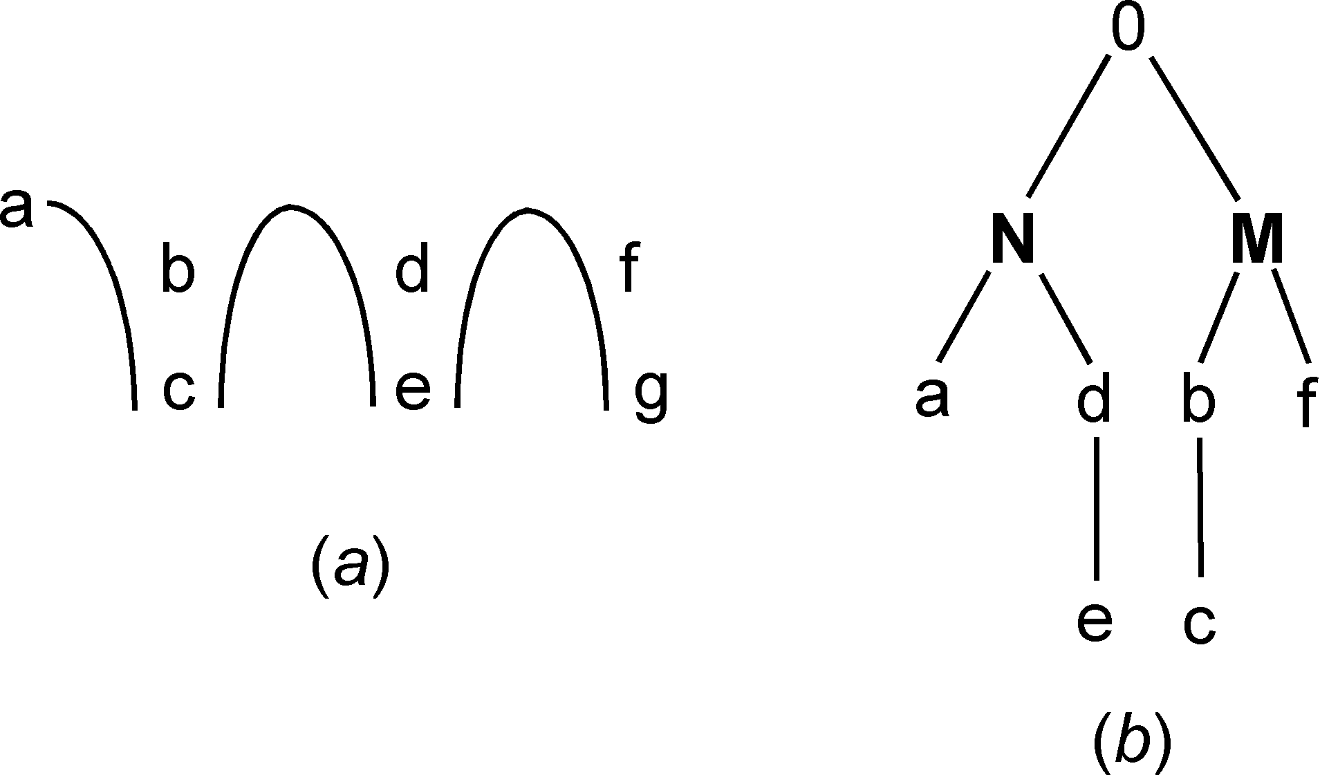
Figure 12. The structure $U$ of Proposition 3.22 (the counter-example) and the O-tree $T$ of Remark 3.23.

Now, we give an example of a structure $U=(N,B)$ that satisfies Properties A1-A6 but is not in IBO_root.

We let $N:=\{a,b,c,d,e,f,g\}$ and $B$ such that $B(a,b,c)$, $B^{+}(c,b,d,e),$ $B^{+}(e,d,f,g)$ hold, and nothing else. See Figure 12(a), using the conventions of Figures 3 and 5. Assume that $B=B_{T}[N]$ where $T$ is an O-tree $(M,\leq)$ such that $N\subseteq M$. We will consider several cases leading each to $B\subset B_{T}[N]$, hence to a contradiction. The relations $<,\leq,\bot$   and $\sqcup$ refer to $T$.

(1) We first assume that $a,c,e,g$ are pairwise incomparable.

The joins $a\sqcup c$, $c\sqcup e$ and $e\sqcup g$ must be defined (because $(a,b,c),(c,b,e)$ and $(e,f,g)$ are in $B_{T}$) and furthermore $b\leq a\sqcup c$, $b\leq c\sqcup e$, $d\leq c\sqcup e$, $d\leq e\sqcup g$ and $f\leq e\sqcup g.$ The joins $a\sqcup c$ and $c\sqcup e$ must be comparable (because $c<\{a\sqcup c,c\sqcup e\})$ and so must be $c\sqcup e$ and $e\sqcup g$.

(1.1) These three joins are pairwise distinct, otherwise $B_{T}[N]$ contains triples not in $B$, as we now prove.

(1.1.1) Assume $a\sqcup c=c\sqcup e=e\sqcup g=\alpha.$ At least one of $a\sqcup e,c\sqcup g$ and $a\sqcup g$ is defined and equal to $\alpha.$

If $a\sqcup e=\alpha=a\sqcup c=c\sqcup e,$ then either $c<d\leq\alpha$ or $e<d\leq\alpha$  because $(c,d,e)\in B_{T}$. Hence, we have $(a,d,c)$ or $(a,d,e)$ in $B_{T}[N]$ but these triples do not belong to $B$. All other proofs will be of this type.

If $c\sqcup g=\alpha=c\sqcup e=e\sqcup g,$ then $(c,f,e)$ or $(c,f,g)$ is in $B_{T}[N]-B$ if, respectively, $e<f\leq\alpha$ or $g<f\leq\alpha$  (because $(e,f,g)\in B_{T}$).

If $a\sqcup g=\alpha=c\sqcup e=e\sqcup g,$ then $(a,f,g)$ or $(c,f,e)$ is in $B_{T}[N]-B$, if, respectively, $g<f\leq\alpha$  or $e<f\leq\alpha$  (because $(e,f,g)\in B_{T}$).

(1.1.2) We now consider the cases where only two of $a\sqcup c$, $c\sqcup e$ and $e\sqcup g$ are equal.

Assume $a\sqcup c=c\sqcup e=\alpha$. If $\alpha<e\sqcup g,$ then $(a,b,g)$ or $(c,b,g)$ is in $B_{T}[N]-B$ (because $(a,b,c)\in B_{T}$); if $e\sqcup g<\alpha,$ then $(c,f,e)$ or $(c,f,g)$ is in $B_{T}[N]-B$ because $\alpha=c\sqcup e=c\sqcup g.$

If $c\sqcup e=e\sqcup g=\alpha$ and $a\sqcup c<\alpha$, then $e<d\leq\alpha$ or $c<d\leq\alpha$ which gives $(a,d,e)$ or $(a,d,c)$ in $B_{T}[N]-B$; if $\alpha<a\sqcup c$, then $(a,f,g)$ or $(a,f,e)$ is in $B_{T}[N]-B$.

If $a\sqcup c=e\sqcup g=\alpha,$ then we have $c\sqcup e<\alpha$ and $a\sqcup e=\alpha.$ Hence, $(a,d,c)$ or $(a,d,e)$ is in $B_{T}[N]-B$. We cannot have $\alpha<$ $c\sqcup e$ because then $c,e<\alpha<c\sqcup e.$

(1.2) If $a\sqcup c$ and $e\sqcup g$ are incomparable, then $a\sqcup c<c\sqcup e$ and $e\sqcup g<c\sqcup e$. We have then $c\sqcup e=c\sqcup g=a\sqcup g$. Hence, we get that $(a,b,g)$ or $(c,b,g)$ is in $B_{T}[N]-B.$

(1.3) Hence, $a\sqcup c$, $c\sqcup e$ and $e\sqcup g$ are pairwise different but comparable. We have six cases to consider : $a\sqcup c<c\sqcup e<e\sqcup g$ and five other ones, corresponding to the six sequences of three objects.

If $a\sqcup c<c\sqcup e<e\sqcup g$ then, $a<b<a\sqcup c$ or $c<b<a\sqcup c$ and $(a,b,g)$ or $(c,b,g)\in B_{T}[N]-B$.

The verifications are similar in the five other cases.

(2) We consider cases where $a,c,e,g$ are not pairwise incomparable.

Observation : If $u<x,(x,y,z)\in B_{T}$ and we do not have $x>z$, then $B_{T}^{+}(u,x,y,z)$ holds. (If $x>z$, then $x$ may not be the join of $u$ and $z$).

If $a>c$, then we have $a>b>c$ and $c\sqcup e>c$. Hence $c\sqcup e\geq b$, or $b>c\sqcup e$. We get triples $(e,b,c)$ or $(a,b,e)$ in $B_{T}[N]-B$.

If $a<c$, then we have $a<b<c\leq c\sqcup e$. Hence $(a,c,e)\in B_{T}[N]-B$.

Hence $a\bot c$. By the observation, we cannot have $e<c,$ $g<c,$ $e<a$ or $g<a$.

If $c<e$, then, if $a\sqcup c\leq e$ we have $(e,b,c)$ or $(e,b,a)$ in $B_{T}[N]-B$; if $e<a\sqcup c$, then $(a,e,c)\in B_{T}[N]-B$.

Hence, $c\bot e$. By the observation, we cannot have $a<c,$ $a<e,$ or $g<e$.

If $e<g$, then, either $c\sqcup e\leq g$ or $g<c\sqcup e$ which gives $(g,b,c)$, $(g,b,e)$ or $(c,g,e)$ in $B_{T}[N]-B$.

Hence, $e\bot g$. By the observation, we cannot have $a<g$ or $c<g$.

All cases yield $B\subset B_{T}[N]$.  Hence, $S$ is not in IBO. ∎

Remarks 3.23.

1. If we modify $U$ of the previous proof by replacing $B^{+}(c,b,d,e)$ by $B^{+}(c,d,e)$ (but we keep $b$ in the set of nodes), we get a modified structure $U^{\prime}$ for which the same result holds, by a similar proof.

2. If we delete $g$ from $U$, we get a structure $W$ that is in IBO_root. A witnessing O-tree $T$ is shown in Figure 12(b) where N and M represent two copies of $\mathbb{N}$ ordered top-down as in the O-tree $T_{2}$ of Figure 8 (cf. the proof of Proposition 2.15).

3. For every finite structure $H=(N_{H},B_{H})$, let $\varphi_{H}$ be a first-order sentence expressing that a given structure $(N,B)$ has an induced substructure isomorphic to $H$. Hence, every structure in IBO satisfies properties A1-A6 and $\lnot\varphi_{U}\wedge\lnot\varphi_{U^{\prime}}$.

We do not know whether this first-order sentence axiomatizes the class IBO, and more generally, whether there exists a finite set of ”excluded” finite induced structures like $U$ and $U^{\prime}$, that would characterize the class IBO. The existence of such a set would give a first-order axiomatization of IBO.

The construction of Theorem 3.21 does not extend to IBO because, as we noted in the proof of Proposition 2.15 (point (3)), a finite structure in IBO may not be an induced betweenness relation of any finite O-tree. No construction like that of $T(\mathcal{C})$ in the proof of Theorem 3.1 can produce an infinite structure from a finite one. Nevertheless:

Conjecture 3.24. The class IBO is characterized by a monadic second-order sentence.

3.3. Logically defined transformations of structures

Each betweenness relation is a structure $S=(N,B)$ defined from a marked O-tree, i.e., a structure $T=(P,\leq,N)$ where $(P,\leq)$ is an O-tree and $N\subseteq P$ , the set of marked nodes, is handled as a unary relation. The different cases are shown in Table 1. In each case a first-order formula can check whether the structure $(P,\leq,N)$ is of the appropriate type, and another one can define the relation $B$ in $(P,\leq,N)$. Hence, the transformation of $(P,\leq,N)$ into $(N,B)$ is a first-order transduction (Definition 1.7).

Structure	Axiomatization	Source	From $(N,B)$ to a
$(N,B)$		structure	source structure
QT	FO : A1-A7, Thm 2.9	join-tree $(N,\leq,N)$	FOT
IBQT	FO : A1-A6, A8, Thm 3.1	join-tree $(P,\leq,N)$	MSOT
BO	MSO : Theorem 3.21	O-tree $(N,\leq,N)$	MSOT
IBO	MSO ? : Conjecture 3.24	O-tree $(P,\leq,N)$	not MSOT

Table 1

The last colomun indicates which type of transduction, FO transduction (FOT) or MSO transduction (MSOT) can produce, from a structure $(N,B),$ a relevant marked O-tree $(P,\leq,N)$. For QT, this follows from the proof of Theorem 2.9(1) : if $S=(N,B)$ satisfies A1-A7 and $r\in N$, then, the O-tree $T(S,r)=(N,\leq_{r})$ is a join-tree and $B=B_{T(S,r)}$. For BO, the MSO sentence that axiomatizes the class constructs a relevant O-tree (it guesses one and checks that the guess is correct). For IBO, we observed that the source tree may need to be infinite for defining a finite betweenness structure, which excludes the existence of an MSO transduction, because these transformations produce structures whose domain size is linear in that of the input structure. (cf. Definition 1.7, and Chapter 7 of [11]).

It remains to prove that the transformation of $S\in$ IBQT into a witnessing marked O-tree $(P,\leq,N)$ is a monadic second-order transduction. This is the content of the following statement.

Theorem 3.25. A marked join-tree witnessing that a given structure $S$ is in IBQT can be defined from $S$ by MSO formulas.

We first describe the proof strategy. We want to prove that, for a given structure $S=(N,B)$ that satisfies Axioms A1-A6 and A8, the tree $T(\mathcal{C})$ of the proof of Theorem 3.1 can be constructed by MSO formulas (of course independent of $S$).

The first step is the construction of $T(S,r)=(N,\leq_{r})$ : one chooses a node $r$ from which the partial order $\leq_{r}$ is FO definable in $S$ by using $r$ as value of a variable. The nodes of $T(\mathcal{C})$ (constructed from $T(S,r)$) are the sets in $\mathcal{C}$ (cf. the proof of Theorem 3.1) and they are of two types :

either $N_{\leq}(z)$, they are in $\mathcal{C}_{1}$,

or $Dir_{L}(u)_{\approx}$ for $u<L$ and $L\in\mathfrak{L}$ such that $Dir_{L}(u)_{\approx}$ is the union of at least two directions (cf. Definition 3.9); they are in $\mathcal{C}_{2}$.

A set $N_{\leq}(z)$ is represented by its maximal element $z$ in a natural way, $T(S,r)$ embeds into $T(\mathcal{C})$ (cf. Section 1.1), and the order between such sets in $T(\mathcal{C})$ is as in $T(S,r)$ by Lemma 3.11(1). A set $Dir_{L}(u)_{\approx}$ is a new node added to $T(S,r)$. In order to make the transformation of $S\longmapsto T(\mathcal{C})$ into a transduction as in Definition 1.7(b), we define $N_{T(\mathcal{C})}$ in bijection with ($N\times\{1\})\uplus(M\times\{2\})$ where $(x,1)$ encodes $N_{\leq}(x)$ and each $w\in M\subseteq N$ encodes (bijectively) some set $Dir_{L}(u)_{\approx}\in\mathcal{C}_{2}$. An MSO formula will express that a node $z$ encodes $U=Dir_{L}(u)_{\approx}$ for some $L$ and $u$.

Lemma 3.10(2) has shown that each set $Dir_{L}(u)_{\approx}$ in $\mathcal{C}_{2}$ can be defined by FO formulas from three nodes $x,y$ and $u$. We need a definition by a single node, in order to obtain a monadic second-order transduction. The sets $U$ in $\mathcal{C}_{2}$ are FO definable but not pairwise disjoint. Hence, one cannot select arbitrarily an element of $U$ to represent it. We will use a notion of structuring of O-trees, that generalizes the one defined in [7] for join-trees, and that we will also use in Section 4. We will also have to prove that the partial order $\leq_{T(\mathcal{C})}$ is defined by MSO formulas, but this will be straightforward by Lemma 3.11, by means of the formula expressing that a node $z$ encodes a set in $\mathcal{C}_{2}$.

Definition 3.26 (Strict upper-bounds). Let $(N,\leq)$ be a partial order and $X\subseteq N.$ A strict upper-bound of $X$ is an element $y$ such that $y>X$, that is, $y\in N_{>}(X)$. We denote by $lsub(X)$ the least strict upper-bound of $X$ if it exists. If $X$ has no maximum element but has a least upper-bound $m$, then $lsub(X)=m.$ If $X$ has a maximum element $m$, its least strict upper-bound if it does exist covers $m,$ that is, $lsub(X)>m$ and there is no $p$ such that $lsub(X)>p>m$.

Definition 3.27 (Structurings of O-trees.). In the following definitions, $T=(N,\leq)$ is an O-tree.

1. If $U$ and $W$ are two lines (convex and linearly ordered subsets of $N$), we say that $W$ covers $U$, denoted by $U\prec W$, if $U<w$ for some $w$ in $W$ and, for such $w$ and any $x\in N$, if $U<x<w,$ then $x\in W$. (See Examples 3.28 below). Note that $lsub(U)$ may not exist, but if it does, it is in $W$.

2. A structuring of $T$ is a set $\mathcal{U}$ of nonempty lines that forms a partition of $N$ and satisfies the following conditions:

   1. One distinguished line called the axis is upwards closed.

   2. There are no two lines $U,U^{\prime}\in\mathcal{U}$ such that $U<U^{\prime}$.

   3. For each $x$ in $N$, $L_{\geq}(x)=I_{k}\uplus I_{k-1}\uplus...\uplus I_{0}$ for nonempty intervals $I_{0},...,I_{k}$ of $(L_{\geq}(x),\leq)$ such that:

      1. $x=\min(I_{k})$  and $I_{k}<I_{k-1}<...<I_{0}$,

      2. for each $j$, there is a line $U\in\mathcal{U}$ such that $I_{j}\subseteq U,$ and it is denoted by $U_{j}$; $U_{0}$ is the axis,

      3. each $I_{j}$ is upwards closed in $U_{j}$, that is, if $x\in U_{j}$ and $x>y\in I_{j}$ then $x\in I_{j}$.

   Hence, $U_{j}\neq U_{j^{\prime}}$ if $j\neq j^{\prime}$, and $U_{j}\prec U_{j-1}$ for $j=1,...,k$. The sequence $I_{0},I_{1},...,I_{k}$ is unique for each $x$, and $k$ is called the depth of $x$ and also of $U_{k}$.  We denote by $U(x)$ the unique line that contains $x\in N.$ We say that $T=(N,\leq,\mathcal{U})$ is a structured O-tree.

Examples 3.28 (On using structurings). The notion of structuring will be used as follows. Consider in an O-tree $T$ a line $L_{>}(x,y)$ defined from incomparable nodes $x$ and $y$. For the construction of MSO transductions, it is essential to define it from a single node. If it has a minimal element $z$, then it is $L_{\geq}(z)$. Otherwise, we can use a structuring $\mathcal{U}$. Assume that the line $U(x)$ is at depth $k$, the line $U(y)$ is at depth $k+1$, $U(y)\prec U(x)$ and $L_{>}(x,y)=$ $U(x)\cap L_{>}(y)$. This latter line is defined in a unique way from $y$ (equivalently, from any $y^{\prime}$ in $U(y)$), and will be denoted by $L^{+}(y).\$Every line in $\mathcal{L}$ is $L^{+}(z)\$for some $z$ (not on the axis). We give examples.

1. The tree $T_{3}$ of Figure 9(a) described in the proof of Proposition 2.15 has several structurings. Its upper part consists of the line $\mathbb{Q}_{>}(\sqrt{2}).$ A first structuring consists of the axis $\mathbb{Q}$ and the two lines $\{a,b\}$ and $\{c,d\}$ at depth 1. Then $\mathbb{Q}_{>}(\sqrt{2})=L_{>}(a,c)=L_{>}(b,c)=L_{>}(c,1)=L^{+}(a)=L^{+}(b)=L^{+}(c)$. A second one consists of $\mathbb{Q}_{>}(\sqrt{2})\cup\{a,b\}$ and the two lines $\mathbb{Q}_{<}(\sqrt{2}):=$ $\mathbb{Q}-\mathbb{Q}_{>}(\sqrt{2})$ and $\{c,d\}$ at depth 1. Then $\mathbb{Q}_{>}(\sqrt{2})=L^{+}(c)=L^{+}(d)=L^{+}(1)$.

2. The rooted tree of Figure 10(b), has a structuring consisting of the axis $\{0,1,a,b\},$ of $\{c,d\}$ and $\{2,e,f\}$ at depth 1 and $\{g,h\}$ at depth 2. We have $\{0\}=L_{>}(a,h)=L^{+}(2)=L^{+}(e)$ and $\{0,2\}=L^{+}(h).$

3. Consider again the join-tree $T:=(Seq_{+}(\mathbb{Q}),$  $\preceq)$ of Examples 1.2(4) and 3.6(2). It has a structuring consisting of the axis $\{(x)\mid x\in\mathbb{Q}\}$ and the lines $\{(x_{1},...,x_{n},z)\mid z\in\mathbb{Q}\}$ for all $x_{1},...,x_{n}\in\mathbb{Q}$. A node $(x_{1},...,x_{n})$ is at depth $n-1$. Then $L^{+}((x_{1},...,x_{n}))$, where $n>1$ is $\{(x_{1},...,x_{n-1},z)\mid z\leq x_{n}\}$.

4. Figure 13 shows a structuring of a join-tree with axis $U_{0}$ and lines $U_{0}$,…, $U_{6}$ such that $U_{1}\prec U_{0},U_{3}\prec U_{2}\prec U_{0}$ $U_{6}\prec U_{2}$ and $U_{5}\prec U_{4}\prec U_{0}$. We have $L_{\geq}(i)=I_{2}\uplus I_{1}\uplus I_{0}$ where $I_{2}=U_{3}\cap L_{\geq}(i),I_{1}=U_{2}\cap L_{\geq}(g),$ $I_{0}=U_{0}\cap L_{\geq}(e).$

   We have $L_{>}(n,m)=L_{>}(g,j)=L^{+}(j).$

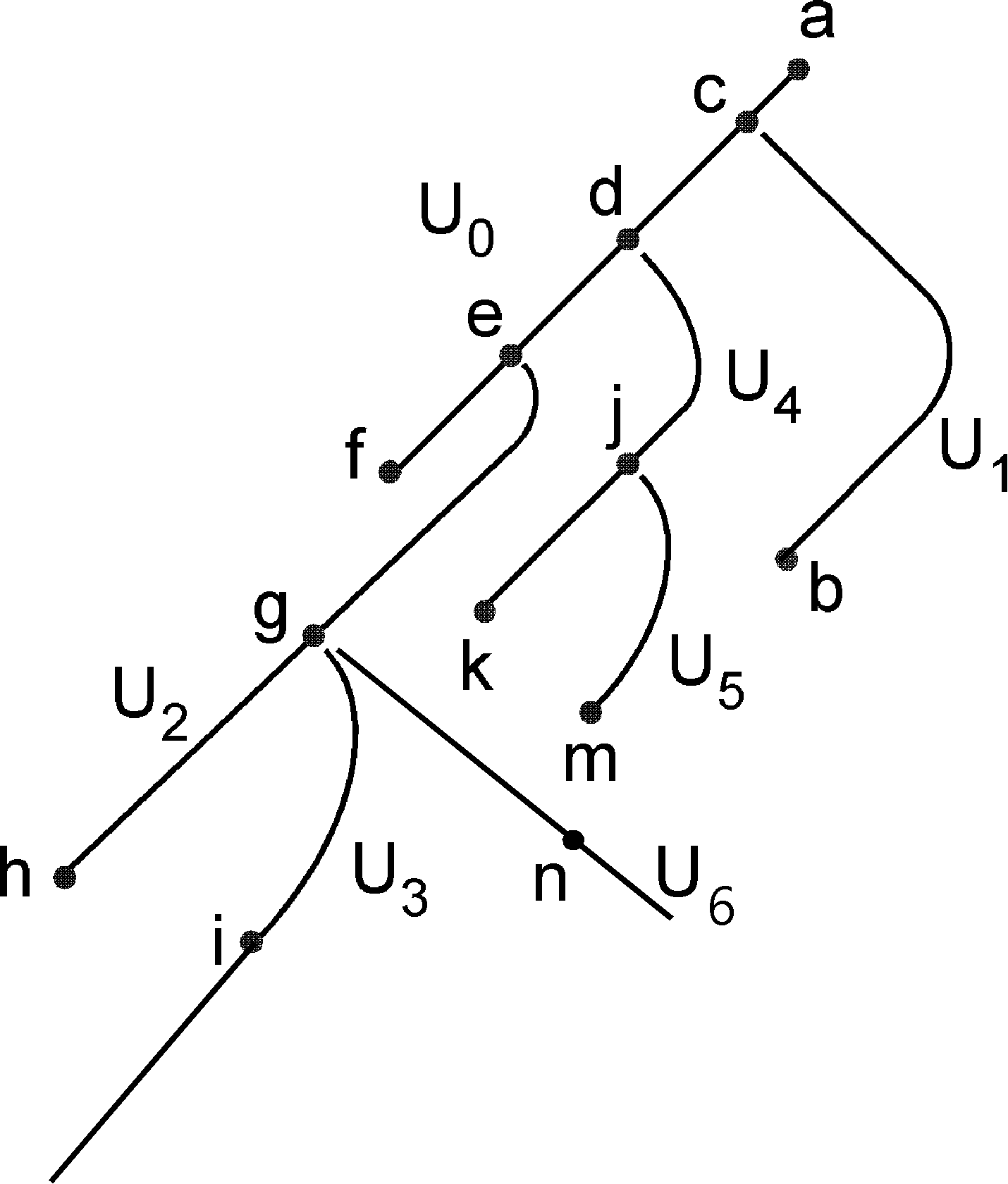
Figure 13. The structuring of Example 3.28(4).

Proposition 3.29. Let $\mathcal{U}$ be a structuring of an O-tree $T=(N,\leq)$. Then, $T$ is a join-tree if and only if each $U\in$ $\mathcal{U}$ that is not the axis has a least strict upper-bound, and $lsub(U)\in W$  where $W$ is the line in $\mathcal{U}$ that covers $U$.

Proof.

Clear from Definition 3.27. ∎

Proposition 3.30. Every O-tree has a structuring.

Proof.

The proof is similar to that of [7] establishing that every join-tree has a structuring. We give it for completeness.  Let $T=(N,\leq)$ be an O-tree. We choose an enumeration $x_{0},x_{1},...,x_{n},...$ of $N$ and a maximal line $B_{0}$; it is thus upwards closed. We define $U_{0}:=B_{0}$. For each $i>0$, we choose a maximal line $B_{i}$ containing the first node not in $B_{i-1}\cup...\cup B_{0}$, and we define $U_{i}:=B_{i}-(U_{i-1}\uplus...\uplus U_{0})$   $=B_{i}-(B_{i-1}\cup...\cup B_{0})$. We define $\mathcal{U}$ as the set of lines $U_{i}$. It is a structuring of $J$. The axis is $U_{0}$. Condition 2) is guaranteed because we choose a maximal line $B_{i}$ at each step. ∎

Lemma 3.31. If $(N,\leq,\mathcal{U})$ is a structured O-tree, we define $S(N,\leq,\mathcal{U})$ as the relational structure $(N,\leq,N_{0},N_{1})$ such that $N_{0}$ is the set of nodes at even depth and $N_{1}:=N-N_{0}$.

1. The class of structures $(N,\leq,N_{0},N_{1})$ that represent a structured O-tree is MSO definable.

2. There is a first-order formula $\nu(X,N_{0},N_{1})$ expressing in every structure $S(N,\leq,\mathcal{U})$ representing a structured O-tree that a set $X$ belongs to $\mathcal{U}$.

Proof.

1. The proof is, up to minor details, that Proposition 3.7(1) in [7]. We let $\sigma(N_{0},N_{1})$ be the corresponding MSO formula.

2. We let $\nu(X,N_{0},N_{1})$ express that:

   (i) $X$ is nonempty, linearly ordered and convex,

   (ii) $X\subseteq N_{0}$ or $X\subseteq N_{1}$,

   (iii) if $x\in N_{0}\cap X$ , $y\in N$ and, $[x,y]\subseteq N_{0}$ or $[y,x]\subseteq N_{0}$, then $y\in X,$

   (iv) the same holds for $N_{1}$ instead of $N_{0}.$

   Let $X\in\mathcal{U}$. Condition 3) of Definition 3.27 yields that, if $x<y$, then $[x,y]\subseteq N_{0}$ or $[x,y]\subseteq N_{1}$ if and only if $x$ and $y$ belong to the same line in $\mathcal{U}$ (in particular because if $[x,y]\subseteq N_{0}$ or $[x,y]\subseteq N_{1}$, then $[x,y]\subseteq I_{k}\subseteq U_{k}).$ Conditions (i)-(iv) hold.

   Conversely, assume that $\nu(X,N_{0},N_{1})$ holds. Let $x\in X.$ We have $X\subseteq U(x)$: let $y\in X$; if $x<y$, then $[x,y]\subseteq N_{0}\cap X\$or $[x,y]\subseteq N_{1}\cap X$. Hence, $y\in U(x)$ by the above remark ; if $y<x$, then, $x\in U(y)$ and so $y\in U(x)$ (because $U(z)$ is the unique line of the structuring that contains $z$).

   If there is $z\in U(x)-X$, then, as $X$ is an interval, we have $z<X$ or $X<z$. The intervals $[z,x]$ (or $[x,z])$ is contained in $N_{0}$ or in $N_{1}$, hence, $z\in X$ by (iii) and (iv). Contradiction. Hence, $X=U(x).$ The formula $x\in X\wedge\nu(X)$ expresses that $X=U(x)$. ∎

Some more notation

Let $T=(N,\leq,\mathcal{U})$ be a structured O-tree with axis $A$. Let $x\in N-A$ and $L_{\geq}(x)=I_{k}\uplus I_{k-1}\uplus...\uplus I_{0}$ as in Definition 3.27(b). We define $L^{+}(x):=I_{k-1}\uplus...\uplus I_{0}.$ We have $U_{k-1}=W_{k-1}\uplus I_{k-1}$ for some interval $W_{k-1}$ of $U_{k-1}$ such that $W_{k-1}<I_{k-1}$. With these hypotheses and notation:

Lemma 3.32.

1. The interval $W_{k-1}$ is not empty.

2. For every $y\in\downarrow(W_{k-1})$, we have $L_{>}(x,y)=L^{+}(x).$

3. Every set $L\in\mathfrak{L}$ is of the form $L^{+}(z)$ for some $z$.

Proof.

1. If $W_{k-1}$ is empty, then $U_{k}<I_{k-1}=U_{k-1}$, contradiction with Condition 2) of Definition 3.27(b).

2. Clear from Condition 2) of Definition 3.27(b).

3. Let $L=L_{>}(x,y)$. We have $L_{\geq}(x)=I_{k}\uplus I_{k-1}\uplus...\uplus I_{0}$ and $L_{\geq}(y)=J_{\ell}\uplus J_{\ell-1}\uplus...\uplus J_{0}$ (cf. Condition 3) of Definition 3.27(b)).  We have three cases:

   Case 1: $I_{m-1}\uplus...\uplus I_{0}=J_{m-1}\uplus...\uplus J_{0}$ for some $m\leq\min(k$,$\ell)$ such that $I_{m}\cap J_{m}=\emptyset.$

   Then $L_{>}(x,y)=L^{+}(z)$ for any $z$ in $I_{m}\cup J_{m}$ (or even in $U_{m}\cup U_{m}^{\prime}$, where $J_{m}\subseteq U_{m}^{\prime}\in\mathcal{L}$). We have also :

   $L_{>}(x,y)=$ $L_{>}(x^{\prime},y^{\prime})=$ $L_{>}(x^{\prime},u)=L_{>}(y^{\prime},u)$ for every $x^{\prime}\in\downarrow(I_{m})$,$y^{\prime}\in\downarrow(J_{m})$ and $u\in\downarrow(U_{m-1}-I_{m-1}))=\downarrow(W_{m-1})$, (cf. (1) and (2)).

   Case 2 : $I_{m-1}\subset J_{m-1}$ and $I_{p}=J_{p}$ for every $p<m-1$.

   Then $L_{>}(x,y)=L^{+}(z)$ for any $z$ in $I_{m}$ (or even in $U_{m}$). We have also

   $L_{>}(x,y)=$ $L_{>}(x^{\prime},u)$ for every $x^{\prime}\in\downarrow(I_{m})$, and $u\in\downarrow(U_{m-1}-I_{m-1})=\downarrow(W_{m-1})$.

   Case 3 : Similar to Case 2 by exchanging $x$ and $y$. ∎

Example and Remarks 3.33.

1. In Case 1, the sets $\downarrow(I_{m}),$ $\downarrow(J_{m})$ and $\downarrow(U_{m-1}-I_{m-1})$ are three different directions relative to $L$. In Case 2, $\downarrow(I_{m})$ and $\downarrow(U_{m-1}-I_{m-1})$ are similarly different directions.

2. In the example of Figure 13, we have :

   $L_{>}(i,n)=L_{>}(h,n)=L^{+}(i)=L^{+}(n)=L_{\geq}(g)$ illustrating Cases 1 and 2,

   $L_{>}(g,m)=L_{>}(h,m)=L^{+}(j)=L^{+}(k)=L_{\geq}(d)$ and

   $L_{>}(k,m)=L^{+}(m)=L_{\geq}(j)$ illustrating Case 2.

Lemma 3.34. There exist FO formulas $\alpha(N_{0},N_{1},r,x,z)$ and $\beta(N_{0},N_{1},r,x,$ $z)$ that express the following properties in a structure $(N,B,N_{0},N_{1},r)$ that satisfies A1-A6 and A8 and defines a structuring of the O-tree $T((N,B),r)$; the corresponding set $\mathcal{C}_{2}$ is as in Definition 3.9.

1. The formula $\alpha(N_{0},N_{1},r,x,z)$ expresses that $x\in L^{+}(z).$

2. The formula $\beta(N_{0},N_{1},r,X,z)$ expresses that $X=Dir_{L^{+}(z)}(z)_{\approx}$ and $X\in\mathcal{C}_{2}$.

Proof.

1. The property $x\in L^{+}(z)$ is expressed by the following FO formula $\alpha(N_{0},N_{1},r,x,z)$  defined as :

   $[z\in N_{0}\wedge\exists y(z<y\leq x\wedge y\in N_{1})]\vee[z\in N_{1}\wedge\exists y(z<y\leq x\wedge y\in N_{0})].$

2. Lemma 3.10(2) shows that the property $X=Dir_{L}(z)_{\approx}\wedge X\in\mathcal{C}_{2}$ is FO expressible provided $x\in L$ is. Assertion (1) shows precisely that $x\in L^{+}(z)$ is FO expressible. ∎

Proof of Theorem 3.25.

By using the previous lemmas, we now prove the existence of MSO formulas that define in a structure $S=(N,B)$ that satisfies A1-A6 and A8, a marked join-tree $T$ such that $N_{T}\supseteq N$ and $B=B_{T}[N]$. In the technical terms of [11] there is a monadic second-order transduction that transforms a structure $S=(N,B)$ into such a marked join-tree ($N_{T},\leq_{T},N$).

The formulas implement the following steps, assuming that $S$ that satisfies A1-A6 and A8.

First step: One chooses $r\in N$, there is no constraint on this choice. One obtains an O-tree $T(S,r)$.

Second step: One guesses a partition $(N_{0},N_{1})$ of $N$ that defines a structuring of $T(S,r)$, according to Lemma 3.31. As the order on $T(S,r)$ depends on $r$, the formula $\sigma(N_{0},N_{1})$ of Lemma 3.31 can be transformed into $\sigma^{\prime}(N_{0},N_{1},r),$ written with $r$ to define $\leq_{r}$.

Third step : All this yields the set $\mathcal{C}=\mathcal{C}_{1}\uplus\mathcal{C}_{2}$ and the associated notions of Definition 3.9 and Lemma 3.32.  We will encode each set in $\mathcal{C}_{2}$ by a unique node $z$ that defines a unique set $Dir_{L^{+}(z)}(z)_{\approx}\in\mathcal{C}_{2}$. We may have $Dir_{L^{+}(z)}(z)_{\approx}=Dir_{L^{+}(w)}(w)_{\approx}$ where $z\neq w$, but we wish to have each set in $\mathcal{C}_{2}$ encoded by a unique node. For insuring this, we choose a set $M$ of nodes such that each set in $\mathcal{C}_{2}$ is $Dir_{L^{+}(z)}(z)_{\approx}\$for a unique node $z\in M$. That a set $M$ is correctly chosen can be checked by using the formula $\beta$ of Lemma 3.34.

We now have the set of nodes of $T(\mathcal{C})$ in bijection with $(N\times\{1\})\uplus$  $(M\times\{2\})$ where $(x,1)$ encodes $N_{\leq}(x)$ and each $w\in M$ in a pair $(w,2)$ encodes a unique set in $\mathcal{C}_{2}$. Hence, we have constructed a structure isomorphic to $T(\mathcal{C})=(N_{T(\mathcal{C})},\leq)$ where $\leq$ is the inclusion of the sets encoded by the pairs in $N_{T(\mathcal{C})}$. This partial order is easy to define by means of the formula $\beta$.

To sum up, the formulas will use the parameters $r,N_{0}$ and $M$ and check they are correctly chosen by existential quantifications :

$r$ to be the root of the O-tree $T(S,r)=(N,\leq_{r})$,

$N_{0}\subseteq N$ such that the structure $(N,\leq_{r},N_{0},N-N_{0})$ represents a structured O-tree,

$M$ intended to be in bijection with $\mathcal{C}_{2}$.

First-order formulas can check that these parameters are correctly chosen. However, the choices of $N_{0}$ and $M$ need set quantifications.

We obtain a join-tree $T^{\prime}$ with set of nodes $N_{T^{\prime}}=(N\times\{1\})\uplus(M\times\{2\})$. Then $S=(N,B)$ is isomorphic to $(N\times\{1\},B_{T^{\prime}}[N\times\{1\}])$ where $(x,1)$ corresponds to $x\in N$. Hence, $S$ is defined by $(N_{T^{\prime}},\leq_{T^{\prime}},N\times\{1\})$ constructed by MSO formulas. ∎

Remark 3.35 (About join-completion). The join-completion builds an O-tree $T$ from the sets $L_{>}(x,y)$ for incomparable $x$ and $y$, cf. Definition 1.3(b). By means of a structuring of $T$, such a set is of the form $L^{+}(z)$, hence can be encoded by a single node $z$. The technique of Theorem 3.25 is applicable to prove that join-completion is an MSO transduction. The join-completion is built with the set of nodes $(N_{T}\times\{1\})\uplus(M\times\{2\})$ where $M$ contains a single node $z$ for each set $L_{>}(x,y)$, where $L^{+}(z)=L_{>}(x,y)$.

4. Embeddings in the plane

In order to give a geometric characterization of join-trees and of induced betweenness in quasi-trees (equivalently, in join-trees), we show how a structured join-tree can be embedded in portions of straight lines in the plane that form a topological tree.

Definition 4.1 (Trees of lines in the plane).

1. In the Euclidian plane, let $\mathcal{L}=(L_{i})_{i\in\mathbb{N}}$ be a family of straight half-lines (simply called lines below) with respective origins $o(L_{i})$, that satisfies the following conditions :

   (i) if $i>0,$ then $o(L_{i})\in L_{j}$ for some $j<i$,

   (ii) for all $i,j\in\mathbb{N}$, $i\neq j$, the set $L_{i}\cap L_{j}$ is $\{o(L_{i})\}$ or $\{o(L_{j})\}$ or is empty. (We may have $o(L_{i})=o(L_{j}))$.

   We call $\mathcal{L}$ a tree of lines : the union of the lines $L_{i}$ is a connected set $\mathcal{L}^{\#}$ in the plane. A path from $x$ to $y\neq x$ in $\mathcal{L}^{\#}$ is a homeomorphism $h$ of the interval $[0,1]$ of real numbers into $\mathcal{L}^{\#}$ such that $h(0)=x$ and $h(1)=y.$ A cycle is a homeomorphism of the circle $S^{1}$ into $\mathcal{L}^{\#}$.

   For any two distinct $x,y\in\mathcal{L}^{\#}$, there is a unique path from $x$ to $y$ (it ”follows the lines”), and consequently, there is no cycle. This path goes through lines $L_{k}$ such that $k\leq\max\{i,j\}$ where $x\in L_{i}$ and $y\in L_{j}$, hence, through finitely many of them. This path uses a single interval of each line it goes through, otherwise, there would be a cycle.

2. We define the ternary betweenness relation:

   $B_{\mathcal{L}}(x,y,z):\Longleftrightarrow\neq(x,y,z)$ and $y$ is on the path between $x$ and $z$.

3. On each line $L_{i}$, we define a linear order as follows:

   $x\preceq_{i}y$ if and only if $y=x$ or $y=o(L_{i})$ or $y$ is between $x$ and $o(L_{i})$.

   On $\mathcal{L}^{\#}$, we define a partial order by:

   $x\preceq y$ if and only if $x=y$ or

   $x\prec_{i_{k}}o(L_{i_{k}})\prec_{i_{k-1}}o(L_{i_{k-1}})\prec_{i_{k-2}}...\prec_{i_{1}}o(L_{i_{1}})\prec_{i_{0}}y$

   for some $i_{0}<i_{1}<...<i_{k}.$ If $k=0$, then $x\prec_{i_{0}}y$.

   It is clear that $(\mathcal{L}^{\#},\preceq)$ is an uncountable rooted O-tree : for each $x$ in $\mathcal{L}^{\#}$, the set $\{y\in\mathcal{L}^{\#}\mid x\preceq y\}$ is linearly ordered with greatest element $o(L_{0})$.

Definition 4.2 (Embeddings of join-trees in trees of lines).

Let $T=(N,\leq,\mathcal{U})$ be a structured join-tree (cf. Definition 3.27). An embedding of $T$ into a tree of lines $\mathcal{L}$ is an injective mapping $m:N\rightarrow\mathcal{L}^{\#}$ such that:

for each $U\in\mathcal{U}$, $m$ is order preserving : $(U,\leq)\rightarrow(L_{i},\preceq_{i})$ for some $i\in\mathbb{N}$, and if $U$ is not the axis, then $m(lsub(U))=o(L_{i}).$

Lemma 4.3. If $T$ is a structured join-tree embedded by $m$ into a tree of lines $\mathcal{L}$, then, its betweenness satisfies:

$B_{T}(x,y,z)\Longleftrightarrow[\neq(x,y,z)\wedge B_{\mathcal{L}}(m(x),m(y),m(z))].$

Proof Sketch.

Let $(x,y,z$)$\in B_{T}$. Assume that $x<y<x\sqcup z$ and let us compare $L_{\geq}(x)=I_{k}\uplus I_{k-1}\uplus...\uplus I_{0}$  and $L_{\geq}(z)=J_{\ell}\uplus J_{\ell-1}\uplus...\uplus J_{0}$ (as in the proof of Lemma 3.32(3)). There are three cases. In each of them, we have a path in $T$ between $x$ and $z$, that goes through $y$ and is a concatenation of intervals of lines of the structuring of $T$. By concatenating the corresponding segments of the lines in $\mathcal{L}$, we get a (topological) path between $m(x)\$and $m(z)$ that contains $m(y).$ Hence, we have $(m(x),m(y),m(z))$ in $B_{\mathcal{L}}.$ The proof is similar in the other direction. ∎

Theorem 4.4. If $\mathcal{L}$ is a tree of lines and $N$ is a countable subset of $\mathcal{L}^{\#}$, then $S:=(N,B_{\mathcal{L}}[N])$ is in IBQT, i.e. is an induced betweenness in a quasi-tree. Conversely, every structure in IBQT is isomorphic to some $S=(N,B_{\mathcal{L}}[N])$ of the above form.

Proof.

If $\mathcal{L}$ is a tree of lines and $N\subset\mathcal{L}^{\#}$ is countable, then $S:=(N,B_{\mathcal{L}}[N])$ is in IBQT. A witnessing join-tree $T$ is defined as follows. Its set of nodes is $N\cup O$ where $O$ is the set of origins of all lines in $\mathcal{L}$. Its partial order is the restriction to $N\cup O$ of the partial order $\preceq$ on $\mathcal{L}^{\#}$. Then $(N,B_{\mathcal{L}}[N])=(N,B_{T}[N])$ hence belongs to IBQT.

Conversely, let $S=(N,B_{T}[N])$ such that $T$ is a structured join-tree. It is isomorphic to $(N,B_{\mathcal{L}}[N])$ for some tree of lines $\mathcal{L}$ by the following proposition. ∎

Proposition 4.5. Every structured join-tree $T$ embeds into a tree of lines $\mathcal{L}$.

The proof will use some notions of geometry relative to positions of lines in the plane.

Definitions 4.6 (Angles and line drawings). An orientation of the plane, say the trigonometric one is fixed.

1. Let $L,K$ be two lines with same origin. Their angle $L\bigtriangleup K$ is the real number $\alpha,$ $0\leq\alpha<2\pi,$ such that $L$ becomes $K$ by a rotation of angle $\alpha$.

   If $o(K)$ is in $L-\{o(L)\}$, we define $L\bigtriangleup K:=L^{\prime}\bigtriangleup K$ where $L^{\prime}$ is the unbounded half-line included in $L$ with origin $o(K).$

2. For a line $L$, an angle $\alpha$ such that $0<\alpha<\pi$ and $O\in L$, we define $S(L,O,\alpha)$ as the union of the lines $K$ with origin $O$ such that $0\leq L\bigtriangleup K<\alpha$. We call sector such a set.

Lemma 4.7. For given $L$ and $\alpha$ as above, one can draw countably many lines with origin $o(L)$ inside the sector $S(L,o(L),\alpha).$

Proof.

We draw $K_{1},K_{2},...,K_{i},...$  such that $L\bigtriangleup K_{1}=\alpha/2$ and $K_{i}\bigtriangleup K_{i+1}=\alpha/2^{i+1}$ for each $i$. ∎

Lemma 4.8. Let $L$, $\alpha$ be as above and $X$ be a countable set enumerated as $\{x_{1},x_{2},...,x_{i},...\}\subseteq L-\{o(L)\}.$ One can draw lines $K_{1},K_{2},...,K_{i},...$ in the sector $S(L,o(L),\alpha)$ in such a way that $o(K_{i})=x_{i}$ for each $i$, no two lines are parallel or meet except at their origins, and none is included in $L$.

Proof.

We must have $0<L\bigtriangleup K_{i}<\alpha$ for each $i$. For each $i$, we let $\gamma_{i}:=\alpha/2^{i+1}$ and $\beta_{i}:=\Sigma\{\gamma_{j}\mid x_{j}\prec x_{i}\}<\alpha$ where $x_{j}\prec x_{i}$ means that $x_{i}$ is between $o(L)$ and $x_{j}$. Then, we draw $K_{1},K_{2},...,K_{i},...$  with respective origins $x_{1},x_{2},...,x_{i},...$ such that $L\bigtriangleup K_{i}=\beta_{i}$. ∎

For each $i$, the sector $S(K_{i},x_{i},\gamma_{i})$ contains nothing else than $K_{i}$. By Lemma 3.8, one can draw inside $S(K_{i},x_{i},\gamma_{i})$ countably many lines with origin $x_{i}$.

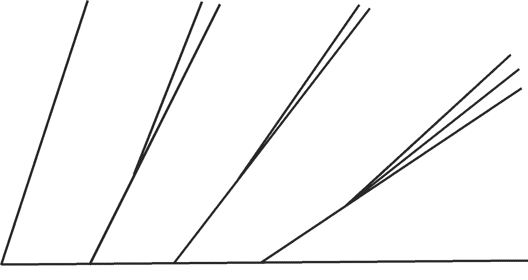
Figure 14. For the proof of Lemma 4.8.

Proof of Proposition 4.5.

Let $\mathcal{U}$ be a structuring of a join-tree $T$. Let $A$ be the axis. Hence, $lsub(A)$ is undefined.

The depth $\partial(U)$ of $U\in\mathcal{U}$ is defined in Definition 3.27 for O-trees. It satisfies the following induction :

• $\partial(A)=0$,

• $\partial(U)=\partial(U^{\prime})+1$ if $U^{\prime}$ has the minimal depth such that $lsub(U)\in U^{\prime}$.

• (Hence, $lsub(U)\neq lsub(U^{\prime})).$

We draw lines $L_{0},L_{1},...$ and define an embedding $m$ such that the conditions of Definition 4.2 hold. We first draw $L_{0}$ and define $m$ on $A$, as required. We choose $\alpha$ such that $0<\alpha<\pi$. All further constructions will be inside the sector $S(L_{0},o(L_{0}),\alpha).$By Lemmas 4.7 and 4.8, we can draw the lines of depth 1. There is space for drawing the lines of depth 2. We continue in this way. ∎

5. Conclusion

We have defined betweenness relations in different types of generalized trees, and obtained first-order or monadic second-order axiomatizations. In Section 4, we have given a geometric characterization of join-trees and the associated betweenness relations.

We have proved that the class IBQT of induced substructures of the first-order class QT of quasi-trees is first-order axiomatizable. This is not an immediate consequence of the FO axiomatization of QT as shown in the appendix.

We conjecture that betweenness in O-trees is not first-order definable (although the class of O-trees is). We also conjecture that the class IBO of induced betweenness relations in O-trees has a monadic second-order axiomatization.

In [7], we have defined quasi-trees and join-trees of different kinds from regular infinite terms, and proved they are equivalently the unique models of monadic second-order sentences. Both types of characterizations yield finitary descriptions and decidability results, in particular for deciding isomorphism. In a future work, we will extend these results to O-trees and to their betweenness relations.

6. Appendix : Induced relational structures

The following example shows that the FO characterization of IBQT does not follow from the FO characterization of the class QT.

Counter-Example 6.1 (Taking induced substructures does not preserve first-order axiomatizability). We prove a little more. We define an FO class $\mathcal{C}$ of relational structures such that $Ind(\mathcal{C})$, the class of induced substructures of those in $\mathcal{C}$, is not MSO axiomatizable.

Let $R$ be a binary relation symbol and $A,B,C$ be unary ones. We let $\mathcal{C}$ be the class of structures $S=(V,R,A,B,C)$ that satisfy the following conditions (i) to (iv) :

1. The sets defined by $A,B,C$ form a partition of $V$,

2. $\forall x,y.(\lnot R(x,x)\wedge[R(x,y)\Longrightarrow\lnot R(y,x)]).$

Hence $S$ can be considered as a directed graph whose vertex set is $V$ and vertices are colored by $A,B$ or $C$. Further conditions are as follows:

1. each infinite connected component of $S$ is a ”horizontal ladder” that is infinite in both directions, and a portion of which is shown in Figure 15; the sets of $A$- and $C$-colored vertices form two biinfinite horizontal directed paths.

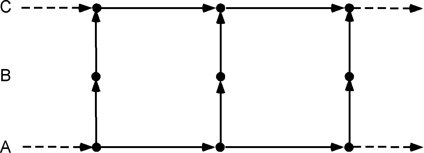
Figure 15. The ladder of Example 6.1.

1. Each finite connected component is a closed ”ring”, with two directed cycles of $A$- and $C$-colored vertices ; Figure 15 shows a portion of such a ring.

By a successor (or predecessor) of $x$, we mean a vertex $y$ such that $(x,y)\in R$ (or $(y,x)\in R$ respectively). Conditions (iii) and (iv) can be expressed by an FO sentence saying in particular:

1. Every vertex $x_{A}$ in $A$ has a unique successor $y_{A}$ in $A$ and a unique successor $x_{B}$ in $B$ ; this vertex $x_{B}$ has a unique successor $x_{C}$ in $C$ ; $y_{A}$ has a unique successor in $y_{B}$ in $B$; $y_{B}$ has a unique successor $y_{C}$ in $C$ that is also the unique successor of $x_{C}$ in $C$.

2. Every vertex in $A$ has a unique predecessor in $A$ and every vertex in $C$ has a unique predecessor in $C$

3. There are no other edges than those specified by (a) and (b).

Let us assume that $Ind(\mathcal{C})$ is characterized by an MSO sentence $\psi$. We will derive a contradiction.

Let $\theta$ be an MSO sentence expressing that a structure $S=(V,R,A,B,C)$ consists of six vertices $x_{A}$, $z_{A}$, $x_{B}$, $z_{B}$, $x_{C}$, $z_{C}$, of directed edges $x_{A}\rightarrow x_{B}$, $x_{B}\rightarrow x_{C}$, $z_{A}\rightarrow z_{B}$ and $z_{B}\rightarrow z_{C}$, of a directed path $p_{A}$ of $A$-colored vertices from $x_{A}$ to $z_{A}$ and of a directed path $p_{C}$ of $C$-colored vertices from $x_{C}$ to $z_{C}$. These conditions imply that $V$ is finite. The construction of $\theta$ is routine. In particular, the existence of paths $p_{A}$ and $p_{C}$ can be expressed in MSO logic with set quantifications. (First-order logic cannot express transitive closures. cf. [11].)

Then, the structures that satisfy $\theta\wedge\psi$ are exactly those that satisfy $\theta$ and have paths $p_{A}$ and $p_{C}$ of equal lengths. But such an equality is not MSO expressible (cf. [11]). Hence, no MSO sentence $\psi$ can characterize $Ind(\mathcal{C})$. ∎

This example shows that the first-order axiomatization of the class IBQT (Theorem 3.1) is not an immediate consequence of the first-order axiomatization of the class QT of quasi-trees. To the opposite, the proof of Proposition 2.12 has used an argument based on the structure of logical formulas.

References

- [1] A. Carayol and S.Wöhrle, The Caucal hierarchy of infinite graphs in terms of logic and higher-order pushdown automata, Proceedings of FST-TCS, Mumbai, India, 2003, pp.112-123.
- [2] O. Carton, T. Colcombet and G. Puppis, An algebraic approach to MSO-definability on countable linear orderings. J. Symb. Log. 83 (2018) 1147-1189.
- [3] M. Changat, P. Narasimha-Shenoi and G. Seethakuttyamma, Betweenness in graphs: A short survey on shortest and induced path betweenness, AKCE International Journal of Graphs and Combinatorics, 16 (2019) 96-109. (Available on ScienceDirect.com, https://doi.org/10.1016/j.akcej.2018.06.007)
- [4] V. Chvatal, Antimatroids, betweenness, convexity, in Research Trends in Combinatorial Optimization, Springer, 2008, pp. 57-64.
- [5] B. Courcelle, Regularity equals monadic second-order definability for quasi-trees, in Fields of Logic and Computation II, Lec. Notes Comput. Sci. 9300 (2015) 129-141.
- [6] B. Courcelle, Several notions of rank-width for countable graphs, J. Comb. Theory, Ser. B. 123 (2017) 186-214.
- [7] B. Courcelle, Algebraic and logical descriptions of generalized trees, Logical Methods in Computer Science 13 (2017) Issue 3.
- [8] B. Courcelle, Betweenness in order-theoretic trees, in Fields of Logic and Computation III, Lec. Notes Comp. Sci. 12180 (2020) 79-94.
- [9] B. Courcelle, Betweenness of partial orders, Theoretical Informatics and Applications, 54 (2020) https://doi.org/10.1051/ita/2020007 (open access).
- [10] B. Courcelle, C. Delhommé, The modular decomposition of countable graphs. Definition and construction in monadic second-order logic. Theor. Comput. Sci. 394 (2008) 1-38.
- [11] B. Courcelle and J. Engelfriet, Graph structure and monadic second-order logic, a language theoretic approach, Cambridge University Press, 2012.
- [12] R. Fraïssé, Theory of relations, Studies in Logic, Volume 145, North-Holland, 2000.
- [13] P. Hlinený, S. Oum, D. Seese, G. Gottlob, Width parameters beyond tree-width and their applications. Comput. J. 51 (2008) 326-362.
- [14] W. Hodges, Model theory, Cambridge University Press, 1993.
- [15] L. Libkin, Elements of finite model theory, Springer, 2004.
- [16] J. Lihova, Strict-order betweenness, Acta Univ. M. Belii Ser. Math. 8 (2000) 27-33. Available from https://actamath.savbb.sk/acta0804.shtml.
- [17] S. Oum, P. Seymour, Approximating clique-width and branch-width. J. Comb. Theory, Ser. B 96 (2006) 514-528.
- [18] P. Parys: Extensions of the Caucal hierarchy, Proceedings of LATA, Lec. Notes in Comp. Sci. 11417, (2019) 368-380.
- [19] W. Thomas, Constructing infinite graphs with a decidable MSO-theory. Mathematical Foundations of Computer Science 2003, Bratislava, Slovakia, Lec. Notes in Comp. Sci 2747, (2003), pp. 113-124